Digital Monopulse Receivers for Phase Modulated Signals Mateo Burgos-García, Gema Ferreiro-Collar, Alberto Asensio López, Javier Gismero Menoyo, Jose Luis Jiménez Grupo de Microondas y Radar Dpto. Señales, Sistemas y Radiocomunicaciones E.T.S.I. Telecomunicación Universidad Politécnica de Madrid Ciudad Universitaria s/n 28040 Madrid, Spain Email:
[email protected]
Abstract— The great success achieved by the monopulse technique in the last years and the fact that the new technology is beginning to allow the construction of digital radar receivers, make us thinking about the digital implementation of the monopulse technique. In this paper different architectures based on amplitude and phase measurement are analyzed. Finally, the results of each architecture are given in some figures.
The log-amplifier of each chain is necessary because accommodates the whole dynamic range and allows the use of a faster A/D converter with smaller number of bits. Finally we will implement our digital monopulse technique in the DSP. I
∆
T
I-Q Demod.
Rx
I. INTRODUCTION
HE monopulse technique has been one of the greatest revolutions introduced for the measurement of the azimuth angle of the targets in the last years. This has been possible because this technique works correctly although the pulses have an internal phase modulation, since it is based on the ratio between the signals Σ and ∆ . Recently, the new technology has begun to allow the construction of digital radar receivers what leads us directly to digital monopulse implementation. The aim of this paper is to show different architectures of digital monopulses when there is a phase modulation with quite bandwidth. Therefore our system will be a pulse compression primary radar that uses a Frank code [1]. The first section describes the receiver general architecture. Then the different implementations of digital monopulses are described, classifying them in architectures based on phase measurement and architectures based on amplitude measurement. Finally the performance of each architecture is analyzed and the results are given in a graphical form.
A/D
∆ digital
A/D
True Log-amplifier DSP I
Σ
I-Q Demod.
Rx
Q
Σ digital
A/D A/D
True Log-amplifier
Fig. 1. Receiver general architecture.
III. ARCHITECTURES BASED ON PHASE MEASUREMENT Architectures based on phase measurement employ 90º hybrid transformers in order to convert an amplitude measurement into a phase measurement. In addition these architectures will need a device for measuring phase differences. A. The quadricorrelator as a device for phase measurement The quadricorrelator is a device for measuring the phase difference between two signals. This process is performed by multiplying one of the signals by the other conjugated. Then this product is integrated in time and finally the phase of the resulting value is the wished phase difference (Fig. 2).
Z1(t)
II. RECEIVER GENERAL ARCHITECTURE Our receiver general architecture is composed by two identical chains for the signals Σ and ∆ ( Fig. 1). These signals are received by a multiple antenna and as we will see later the receivers can introduce some imperfections in a real case.
0-7803-7871-7/03/$17.00 © 2003 IEEE
Q
Z2(t)
Z*
∫ · dt
Phase ( )
Fig. 2. Block diagram of the quadricorrelator.
640
Radar 2003
Form Approved OMB No. 0704-0188
Report Documentation Page
Public reporting burden for the collection of information is estimated to average 1 hour per response, including the time for reviewing instructions, searching existing data sources, gathering and maintaining the data needed, and completing and reviewing the collection of information. Send comments regarding this burden estimate or any other aspect of this collection of information, including suggestions for reducing this burden, to Washington Headquarters Services, Directorate for Information Operations and Reports, 1215 Jefferson Davis Highway, Suite 1204, Arlington VA 22202-4302. Respondents should be aware that notwithstanding any other provision of law, no person shall be subject to a penalty for failing to comply with a collection of information if it does not display a currently valid OMB control number.
1. REPORT DATE
2. REPORT TYPE
14 APR 2005
N/A
3. DATES COVERED
-
4. TITLE AND SUBTITLE
5a. CONTRACT NUMBER
Digital Monopulse Receivers for Phase Modulated Signals
5b. GRANT NUMBER 5c. PROGRAM ELEMENT NUMBER
6. AUTHOR(S)
5d. PROJECT NUMBER 5e. TASK NUMBER 5f. WORK UNIT NUMBER
7. PERFORMING ORGANIZATION NAME(S) AND ADDRESS(ES)
Grupo de Microondas y Radar Dpto. Señales, Sistemas y Radiocomunicaciones E.T.S.I. Telecomunicación Universidad Politécnica de Madrid Ciudad Universitaria s/n 28040 Madrid, Spain 9. SPONSORING/MONITORING AGENCY NAME(S) AND ADDRESS(ES)
8. PERFORMING ORGANIZATION REPORT NUMBER
10. SPONSOR/MONITOR’S ACRONYM(S) 11. SPONSOR/MONITOR’S REPORT NUMBER(S)
12. DISTRIBUTION/AVAILABILITY STATEMENT
Approved for public release, distribution unlimited 13. SUPPLEMENTARY NOTES
See also ADM001798, Proceedings of the International Conference on Radar (RADAR 2003) Held in Adelaide, Australia on 3-5 September 2003. 14. ABSTRACT 15. SUBJECT TERMS 16. SECURITY CLASSIFICATION OF: a. REPORT
b. ABSTRACT
c. THIS PAGE
unclassified
unclassified
unclassified
17. LIMITATION OF ABSTRACT
18. NUMBER OF PAGES
UU
6
19a. NAME OF RESPONSIBLE PERSON
Standard Form 298 (Rev. 8-98) Prescribed by ANSI Std Z39-18
B. Phase architecture nº 1 This architecture employs two hybrid transformers to generate the signals Σ+j∆ and Σ-j∆ from Σ and ∆ , and once they have been digitalized it uses the quadricorrelator to calculate the phase difference between them (Fig. 3).
∆ digital Σ digital
Σ+j∆ Signal formation
Z*
∫ · dt
Σ−j∆
Phase ( )
1 2
tg ( )
1 k
θ
quadricorrelator
Fig. 3. Block diagram of phase architecture nº 1.
IV. ARCHITECTURES BASED ON AMPLITUDE MEASUREMENT These architectures perform the azimuth angle estimation by evaluating the relative amplitudes of the signals coming from the aerial system. So once we have the ratio between the beam patterns ∆ and Σ we can obtain the azimuth angle of the targets using the relation expressed in (2). Here we are going to describe three different techniques for implementing a digital monopulse based on amplitude measurement. In all the cases the sign of the angle will be derived from the phase relationship between the signals by means of the quadricorrelator described in section III.A. A. Amplitude architecture nº 1 The block diagram of this architecture is shown in Fig. 5.
Since the estimation equation [2] has the form:
∑ + j∆ ∆ 1 = arg ∑ 2 ∑ − j∆
Arc tg
(1)
we can evaluate the ratio between Σ and ∆ using the quadricorrelator and then obtain the azimuth of the targets using:
∆ = kθ ∑
Σ digital
Σ+j∆
Z*
Σ
Average
Σ digital
|·|
Average
1 Gcad
1 k
Natural units
θ
Z*
∫ · dt
Re ( )
Sign ( )
quadricorrelator
Fig. 5. Block diagram of amplitude architecture nº 1
C. Phase architecture nº 2 This architecture employs only one hybrid transformer to generate the signals Σ+j∆ and Σ, and also uses the quadricorrelator to calculate the phase difference between the digitalized signals (Fig. 4).
Signal formation
|·|
(2)
feature that holds near the center line (boresight) of any model of the aerial system.
∆ digital
∆ digital
∫ · dt
Phase ( )
tg ( )
1 k
In this case the modulus of the azimuth angle of the targets is obtained by subtracting the averaged moduli of the signals coming from each receiver chain, dividing by the gain of the system, converting the result to natural units due to the presence of the logarithmic amplifiers in the receiver chains and dividing by the constant k, which depends on the relation between the antenna patterns. The time averaging operation is performed along one Frank code. Finally the sign of the angle is obtained by means of the quadricorrelator that has been modified slightly as we can see in Fig. 5.
θ
B. Amplitude architecture nº 2 The block diagram of this architecture is shown in Fig. 6.
quadricorrelator
Fig. 4. Block diagram of phase architecture nº 2
∆ digital
Restoration of true modulus
Σ digital
Restoration of true modulus
In this case, the estimation equation [2] has the form:
∆ ∑ + j∆ Arc tg = arg ∑ ∑
(3)
1 Gcad
..
Average
1 Gcad
|·|
1 k
θ
Z*
∫ · dt
and again we can evaluate the ratio between Σ and ∆ using the quadricorrelator and then obtain the azimuth of the targets using (2).
Re ( )
Sign ( )
quadricorrelator
Fig. 6. Block diagram of amplitude architecture nº 2
641
The main difference between this architecture and the previous one is that now we neutralise the logarithmic amplifiers of the receiver chains. Since their presence is very important to accommodate the whole dynamic range of the system to the ADC’s, what we really do is incorporate a new block with their inverse behaviour, using the 16-bit dynamic range of the DSP’s. In this case the modulus of the azimuth angle is obtained by dividing the signals coming from the receiver chains, which have been divided by the gain of the system, and then averaging, taking the modulus of the result and dividing by the constant k. Note that in this case the quotient is performed between two complex signals (they keep their phase modulation in this point), and so is the time-averaging operation. Again the sign of the angle is obtained using the modified quadricorrelator. C. Amplitude architecture nº 3 The block diagram of this architecture is shown in Fig. 7. correlator
∆ digital
Amplitude (∆) 1 Gcad
Frank Code
Σ digital correlator
Natural units
1 k
Amplitude (Σ)
θ
Z*
∫ · dt
Re ( )
Sign ( )
quadricorrelator
Fig. 7. Block diagram of amplitude architecture nº 3
The third amplitude architecture uses the code information of the signals because it is based on the despreading of them. The despreading consist in correlating the signals coming from each of the receiver chains with the Frank code used in their modulation, obtaining as a result values proportional to the amplitude of the signals Σ and ∆ . For this process it is very important that the modulation was a phase modulation, thus we can maintain the logarithmic since there is no dependency with the moduli of the signals. After the despreading we subtract the resulting values, divide by the gain of the system, convert the result into natural units and finally divide by the constant k. As in the previous cases, the sign of the angle comes from the modified quadricorrelator.
Some of them are phase noise, group delay or amplitude and phase imbalances between the I-Q components. Firstly we will consider that all these imperfections are negligible and we will analyze only the thermal noise effects. Figures 8-12 show the azimuth angle estimation error of each architecture for a signal to noise ratio of 20 dB, optimal value in which it is thought these systems work. Figures 8 and 9 show that for architectures based on phase measurement the estimation error is low for normalized azimuth angles next to zero and it grows as we move away from the boresight. If we compare the estimation error of both architectures we observe that it has the same behavior but with larger value in architecture nº 2. Figure 10 shows the estimation error for amplitude architecture nº 1, as we can see its value is very high for normalized azimuth angles next to zero. Usually it is said that this is due to the sign estimator, whose error probability is much larger near the boresight. However, this behaviour is due to the own architecture operation because as we have seen the other amplitude architectures use the same sign detector, the quadricorrelator, but their estimation error is much smaller (Fig. 11) and even null (Fig. 12) near the boresight. Fig. 11 shows that the estimation error in amplitude architecture nº 2 is the same than in amplitude architecture nº 1 but with smaller error in the boresight. Finally, in Fig. 12 we observe that the behaviour of amplitude architecture nº 3 is opposed to the others amplitude architecture behaviours, because its error is null near the boresight and very high in the rest of the normalised angles. Therefore, the architecture that works better for very small normalized azimuth angles is the amplitude architecture nº 3, whereas the one that works worse is the amplitude architecture nº 1. However, these behaviour are reversed as soon as we separate a little from the boresight, where amplitude architecture nº 1 has the lowest estimation error coinciding with amplitude architecture nº2 and phase architecture nº 1 estimation errors.
V. ANALYSIS AND RESULTS A. Ideal Case: without system imperfections In the receiver general architecture described in section II it is possible that diverse imbalances due to the system imperfections appear.
Fig. 8. Azimuth angle estimation error in phase architecture nº 1 for θB=3.3º, θM=2º and η=0.7
642
Fig. 9. Azimuth angle estimation error in phase architecture nº 2 for θB=3.3º, θM=2º and η=0.7
Fig. 10. Azimuth angle estimation error in amplitude architecture nº 1 for θB=3.3º, θM=2º and η=0.7
Fig. 12. Azimuth angle estimation error in amplitude architecture nº 3 for θB=3.3º, θM=2º and η=0.7
B. Effect of system imperfections Now we consider the different non idealities that can appear in the system. Firstly, we will describe them briefly and we will see their values within a real system. Then we will analyse the azimuth angle estimation error again. Phase noise. It is generated by the oscillators in the system, Fig. 13 shows the phase noise considered in all the architectures. Group delay. It is due to the filters in the system, Fig. 14 shows the group delay considered in all the architectures. Amplitude and phase imbalances between the I-Q components. They are generated by the own I-Q demodulator operation. We will consider an amplitude imbalance of 1 dB and a phase imbalance of 2 degrees. Figures 15-19 show the azimuth angle estimation error of each architecture for the values mentioned of the system imbalances and a signal to noise ratio of 20 dB.
Fig. 11. Azimuth angle estimation error in amplitude architecture nº 2 for θB=3.3º, θM=2º and η=0.7
Fig. 13. Oscilator phase noise in all the architectures
643
Fig. 14. Group delay in all the architectures
Fig. 17. Azimuth angle estimation error in amplitude architecture nº 1. Comparison between the real and the ideal case.
Fig. 15. Azimuth angle estimation error in phase architecture nº 1. Comparison between the real and the ideal case.
Fig. 18. Azimuth angle estimation error in amplitude architecture nº 2. Comparison between the real and the ideal case.
Fig. 16. Azimuth angle estimation error in phase architecture nº 2. Comparison between the real and the ideal case.
Fig. 19. Azimuth angle estimation error in amplitude architecture nº 3. Comparison between the real and the ideal case.
644
In all the cases we observe the estimation error in a real case is larger than in an ideal one, but whereas in some architectures the difference is very small in others it has a considerable value. If we notice the imbalances we are considering we see that all of them affect the phase of the signals, only the imbalances between the I-Q components affects the phase and the amplitude. Therefore, architectures based on phase measurement will be more affected that those that are based on amplitude measurement. In Figures 15 and 16 we can see the azimuth angle estimation error of both phase architectures, as we expected the error experiments an important growth when we consider the system imperfections. If we analyse separately the different imbalances we would observe that what affects the most to phase architecture nº 1 are I-Q imbalances, whereas what affects the most to phase architecture nº 2 are the imbalances along with phase noise. If we notice Figures 17 and 18 we observe that amplitude architectures nº 1 and 2 are not affected by the imbalances. As we have commented before only I-Q imbalances could increase the estimation error in these cases, but the real values of these imbalances are so small that they do not have almost any effect on the behaviour on these architectures. Finally, in Figure 19 we see that amplitude architecture nº 3 is strongly affected by system imbalances, what can seem strange since this architecture is based on amplitude measurement as the previous ones. This is because this architecture uses the despreading of the signals to estimate their amplitude, as we saw in section IV.C it consists in correlating the digitalized signals with the Frank code used in their modulation and this process depends on the phase. If we analysed separately the different system imbalances we would observe that what affects the most to this architecture is the group delay. We observe that in all the cases the effects of system imperfections are larger as we move away from the boresight, this is specially notable in Fig 19 corresponding to amplitude architecture nº 3. We can also see that this architecture is the most affected by system imperfections mainly for high normalised angles.
In a real case, phase architecture nº 1 has the same estimation error than amplitude architectures nº 1 and nº 2 but with a lower error in the boresight. The disadvantage of this architecture is that it is affected by systems imbalances. Finally, phase architecture nº 2 has an estimation error parallel to the other phase architecture error, thus its behaviour is the same but its value is larger, but without surpassing the estimation error of amplitude architecture nº 3 except near the boresight. This architecture is also affected by the system imperfections. We can conclude that the optimal architecture would be the one that behaves as amplitude architecture nº 3 for values near the boresight, where this architecture has the lowest estimation error and is not affected by system imperfections, and behaves as amplitude architecture nº 2 for the rest of the normalised angles, where this architecture has the lowest estimation error and is not affected by system imperfections. Therefore, a new digital monopulse technique could be designed whose operation would depend on the azimuth angle of the targets. VII. ACKNOWLEDGMENT This work has been done thanks to the finantial support of the CICYT TIC2002-04569-C02-01. VIII. REFERENCES [1] [2] [3] [4]
VI. CONCLUSIONS We observe that amplitude architectures nº 1 and nº 2 present the better behaviour with respect to system imperfections, in addition their azimuth angle estimation errors are the minimum among of all architectures except near the boresight where the estimation error of amplitude architecture nº 1 is specially elevated. For normalized azimuth angles very next to zero amplitude architecture nº 3 presents the smallest estimation error of all, however when we move away from the origin its error becomes the highest, becoming still larger in presence of imbalances. Moreover, this architecture is the most affected by the system imperfections .
645
Bernard L. Lewis, Frank F. Kretschmer, and Wesley W. Shelton, Aspects of Radar Signal Processing. Artech House, INC: Norwood, 1986, pp. 9, 11, 14-15, 23-26. Hofstetter, E.M., and De Long, D.F., “Detection and parameter estimation in an amplitude-comparison monopulse radar,” IEEE Transactions on Information Theory, IT-15, pp. 22-30, January 1969. Jacovitti, G., “Performance analysis of monopulse receivers for secondary surveillance radar,” IEEE Transactions on Aerospace and Electronic Systems, vol. AES-19, nº 6, November 1983. Jha, A.R., “High performance analog-to-digital converters (ADCs) for signal processing,” 2nd International Conference on Microwave and Millimeter Wave Technology, pp. 32-35, 2000.