904
IEEE TRANSACTIONS ON AUTOMATIC CONTROL, VOL. 57, NO. 4, APRIL 2012
Distributed Seeking of Nash Equilibria With Applications to Mobile Sensor Networks Miloˇs S. Stankovic´, Karl H. Johansson, and Duˇsan M. Stipanovic´
Abstract—We consider the problem of distributed convergence to a Nash equilibrium in a noncooperative game where the players generate their actions based only on online measurements of their individual cost functions, corrupted with additive measurement noise. Exact analytical forms and/or parameters of the cost functions, as well as the current actions of the players may be unknown. Additionally, the players’ actions are subject to linear dynamic constraints. We propose an algorithm based on discrete-time stochastic extremum seeking using sinusoidal perturbations and prove its almost sure convergence to a Nash equilibrium. We show how the proposed algorithm can be applied to solving coordination problems in mobile sensor networks, where motion dynamics of the players can be modeled as: 1) single integrators (velocity-actuated vehicles), 2) double integrators (force-actuated vehicles), and 3) unicycles (a kinematic model with nonholonomic constraints). Examples are given in which the cost functions are selected such that the problems of connectivity control, formation control, rendezvous and coverage control are solved in an adaptive and distributed way. The methodology is illustrated through simulations. Index Terms—Convergence, extremum seeking, learning, mobile sensor networks, multi-agent control, Nash equilibrium, noncooperative games, stochastic optimization.
I. INTRODUCTION
P
ROBLEMS of distributed, multi-agent optimization, coordination, estimation, and control have been the focus of significant research in past years. Depending on the problem setup and the available resources, agents may have access to different measurements, different a priori information, such as system models and sensor characteristics, and different interagent communication channels. A possible approach to these problems is game theoretic, where one formulates a noncooperative game with players/agents selfishly trying to optimize their individual cost functions by using locally available information. Depending on the structure of the game, its Nash equilibria can Manuscript received August 02, 2010; revised January 25, 2011; accepted October 24, 2011. Date of publication November 03, 2011; date of current version March 28, 2012. This work was supported in part by the Knut and Alice Wallenberg Foundation, in part by the Swedish Research Council, in part by the Swedish Strategic Research Foundation, and in part by the EU project FeedNetBack. Parts of this work have been presented in a preliminary form in [1]. Recommended by Associate Editor J. Cortes. M. S. Stankovic´ and K. H. Johansson are with the ACCESS Linnaeus Center, School of Electrical Engineering, KTH Royal Institute of Technology, 100-44 Stockholm, Sweden (e-mail:
[email protected];
[email protected]). D. M. Stipanovic´ is with the Department of Industrial and Enterprise Systems Engineering and the Coordinated Science Laboratory, University of Illinois at Urbana-Champaign, Urbana, IL 61801 USA (e-mail:
[email protected]). Color versions of one or more of the figures in this paper are available online at http://ieeexplore.ieee.org. Digital Object Identifier 10.1109/TAC.2011.2174678
have different properties and they may or may not correspond to the optimal solution of some global optimization problem [2]–[10]. The focus of this paper is on the problem of learning in games, or designing algorithms that converge to a Nash equilibrium. The majority of the existing literature in this area is focused on algorithms based on a detailed model of the underlying game; that is, an algorithm is designed based on a specific form of the players’ cost functions and properties. Furthermore, it is usually assumed that the players can observe the actions of the other players. In this way, the algorithms can be designed on the basis of a best/better response strategy. For example, in [11], convergence properties have been analyzed for such a class of infinite, convex games. For games with finite action sets, where the players can use mixed strategies, the convergence of the underlying best response algorithm, called fictitious play, and its modifications have been analyzed intensively (see [12] and references therein). The recently proposed algorithms in [13] and [14] deal with an information structure similar to the one imposed in this paper, but require synchronization between the agents, and the convergence is proved only for a special class of games (weakly acyclic or potential games [4]) with finite action sets. In [15] an interactive learning procedure based on trial and error is proposed. A similar approach to the one proposed in this paper, applied to quadratic games in markets, has appeared independently in [16] and extended to non-quadratic cost functions in [17], but the authors provided only local stability analysis of a simpler one-dimensional scheme under strong conditions. Also, none of the mentioned approaches can deal with the measurement noise while taking into account specific dynamics of the players. Extremum seeking algorithms have received significant attention recently in adaptive online optimization problems involving dynamical systems. The basic algorithm, based on introducing sinusoidal perturbations, has been treated in, e.g., [18]–[20]. In [21] and [22] a time-varying version of the algorithm has been introduced, whose almost sure convergence has been proved in the presence of measurement noise. It has been demonstrated how this technique can be applied to autonomous vehicles seeking a target in deterministic environments [23], or optimal positioning in stochastic environments [22], [24]. In this paper, we propose a discrete-time algorithm for distributed seeking of a pure Nash strategy in infinite games where the players generate their actions based solely on the measurements of their individual cost functions, whose detailed analytical forms may be unknown. Furthermore, similarly as in the extremum seeking problems, we assume that the players may have some (possibly unknown) linear dynamics , filtering the players’
0018-9286/$26.00 © 2011 IEEE
´ et al.: DISTRIBUTED SEEKING OF NASH EQUILIBRIA WITH APPLICATIONS TO MOBILE SENSOR NETWORKS STANKOVIC
actions before affecting their cost functions. Also, the local measurements of individual cost functions are not available directly, they are filtered through a stable filter and corrupted with measurement noise. The proposed algorithm is based on the timevarying extremum seeking algorithm with sinusoidal perturbations, under stochastic noise, analyzed in [22]. We formulate sufficient conditions on the structure of the cost functions and on the parameters of the proposed scheme, under which we prove almost sure convergence to a Nash equilibrium. Some important special cases (potential games and quadratic games), and possible extensions and limitations are treated in details. The proposed algorithm can be applied to general noncooperative games in which there is a need for adaptive learning of Nash equilibria; that is, when the players may not know the exact parameters of the cost functions and the current players’ actions and properties, or even if they do not know the exact analytical forms of the costs, but are able to obtain (noisy) values of their individual costs at each time instance. The players may also have some dynamics which imply certain constraints on their capability of changing actions. These properties make the algorithm appealing for distributed coordination and optimization problems related to mobile sensor networks. These networks are usually deployed in some only partially known or unknown and noisy environments, lacking any communication infrastructure and without some omniscient central or fusion node. The information that the agents have about the environment as well as about the actions/properties of the other agents is limited only to certain local sensing and local low bandwidth communications. In certain scenarios, the individual cost for each agent can be expressed as a sum of a locally defined goal, depending only on the individual agent’s position/action (such as the one treated in [22], [24], or [23]) and a “collective” goal, depending on the positions/actions of the other agents. This is typical in connectivity control problems [25]–[28]. By applying our scheme to such problems the agents can adaptively achieve a compromise between these locally defined goals, and a “collective” goal of maintaining connectivity with the neighboring agents, without detailed inter-agent communications and without position measurements. We show that a special case of this scenario leads to an adaptive solution of a formation control problem and a rendezvous or consensus problem (see, e.g., [29], [30], and references therein). In some cases a cooperative control task to be performed by a mobile network is expressed using a global cost function which may depend on all the environmental parameters and properties/positions of all the agents. In these cases, to deal with the agents’ lack of global information it is possible to design individual cost functions which would capture the given information structure constraints. The design should be done such that local optimizations by individual agents (Nash equilibrium) leads to an optimum of a global objective [3], [4], [9], [10]. Even though the cost functions are designed, they usually depend on some parameters/functions (e.g., environmental conditions, individual agents’ properties) which are unknown a priori and must be learned (implicitly or explicitly) in the process of convergence to a Nash equilibrium. A typical example for this scenario is a coverage control problem as defined in [31] and formulated as a potential game in [32]–[34]. Using our methodology, this
905
problem can be solved under much more realistic assumptions on the information available to the agents. Specifically, in our setting, the agents do not need any (absolute or relative) position measurements and do not need a priori knowledge about the distribution of the events to be detected (environmental density function) and about the specific detection capabilities of the individual agents. The existing literature in the area of mobile sensor networks which treats similar problems is mostly focused on specific scenarios requiring detailed sensing/comunication models as well as the model of the environment, without taking specific mobile robot dynamics into consideration (e.g., [14], [25]–[28], [30]–[32], [35]–[38] and references therein). The rest of the paper is organized as follows. In Section II the problem setup and the algorithm description are given. Section III is devoted to the convergence analysis, where we prove that the algorithm converges almost surely (a.s.) to a Nash equilibrium. We discuss possible extensions, limitations and special cases in Section IV. In Section V, we give detailed analysis of some concrete applications of the proposed algorithm to mobile sensor networks (connectivity control, formation control, rendezvous and coverage control), where the dynamics of the mobile robots can be modeled as single integrators, double integrators or unicycles. Simulation results for networks of three agents are shown and discussed. II. NASH EQUILIBRIUM SEEKING ALGORITHM agents are noncooperWe consider a scenario in which atively minimizing their individual cost functions by updating their local actions, based only on their current local informa, tion. We assume that the actions of the players belong to , . Hence, we are dealing with a noncooperative static game with infinite action spaces where the optimality is characterized by a (pure) Nash equilibrium; a point from which neither agent has incentive to deviate [2], [5]. We assume that the information that each player has about the underlying game is restricted solely to discrete-time measurements of its individual cost function, which are, in addition, filtered through (possibly unknown) stable, linear and time inand corrupted variant (LTI) filter with transfer function with a measurement noise. The players may not have any direct information about either the underlying structure of the game (exact analytical forms of the cost functions) or the actions/properties of the players. Without loss of generality, let us assume that each agent’s action space is two-dimensional, , since we will apply this methodology to vehicles’ coordination problems in the plane. The framework can be extended to multidimensional action spaces in a straightforward way, as discussed later in Remark 5. Furthermore, the agents may have some local dynamics, so that their actions are filtered through (possibly unknown) stable LTI filter, having the , before affecting the measured transfer function matrix , where denotes the accost function denotes the actions of all the other tion of agent , while agents. In general, each cost function does not necessarily have to depend on the actions of all the other players. So, let , whose us define time-invariant neighbor sets ,
906
IEEE TRANSACTIONS ON AUTOMATIC CONTROL, VOL. 57, NO. 4, APRIL 2012
In what follows we are going to introduce assumptions needed for proving the convergence of the algorithm to a Nash equilibrium. Assumption On the Measurement Noise: (where (A.1) The random vectors ) are measurable with respect to , mutually independent a flow of -algebras and zero mean, and they satisfy (6) Fig. 1. Nash equilibrium seeking scheme.
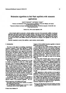
elements are indices of the agents whose actions affect the th agent’s cost function. Motivated by the fact that the formulated information structure relates to extremum seeking problems, we propose an algorithm based on sinusoidal perturbations, depicted in Fig. 1, where each agent implements a local, discrete-time (denoted by ), extremum seeking loop. The estimation of the gradient of the individual cost function is performed by inserting a sinuand with positive, desoidal perturbation, with frequency , which, by passing terministic, time-varying amplitude through the function , is being modulated by its local slope. The estimate of the slope is found by the multiplication/demodulation using the sinusoid with the same frequency and with pos. This slope itive, deterministic, time-varying amplitude estimate is then used to move in the opposite direction (by the ). Since all the information negative integration block: needed to estimate the gradient is located in the amplitude of the modulated sinusoidal perturbation, the measurements are filto eliminate any DC components, tered by washout filters and, hence, to improve the overall convergence properties. Also, to improve the convergence properties, low-pass filters can be . Local decouadded in the loop as part of the dynamics pling between and dimensions is obtained using orthogonal perturbations: cosine for and sine for (cf., [24] or [23]). Furthermore, neighboring agents apply different frequency pertur, , so that decoupling between their bations, gradient estimates is achieved. The following equations model the behavior of the proposed Nash equilibrium seeking algorithm: (1) (2) (3) for agent
, where
is the measurement noise of
(4) (5) denotes a time Throughout the paper, the expression domain vector obtained as the output of LTI system with the transfer function matrix , with the input vector , and with some arbitrary finite initial condition.
, ( denotes mathfor some matrix means that the ematical expectation, the notation is positive semidefinite, denotes any matrix matrix norm). Assumptions On the Parameters of the Algorithm: are decreasing, (A.2) The scalar sequences , and , . are decreasing, (A.3) The scalar sequences , and , . , . (A.4) for all and (A.5) . (A.6) for all and . when , for all (A.7) . (A.8) , is a rational number, and for all and . can be written as According to (A.7), (7) for each and for some constants . Assumptions (A.2)–(A.6) are standard assumptions on the step size in recursive, stochastic and deterministic (sub)gradient and extremum seeking algorithms (see, e.g., [22], and [39]–[42]). They aim at reducing the effect of measurement noise; however, to achieve convergence of the algorithm, these parameters need to converge to zero slow enough so that (A.4) is satisfied. A straightforward way of satisfying Assumptions (A.2)–(A.7) is by simply taking and where , , , and and can account for asynchronicity between the agents. Assumption on the Existence of a Nash Equilibrium: are contin(A.9) The individual cost functions uously differentiable and strictly convex in local decision variables , and there exists a Nash equilibrium, i.e., a for which the following holds: point (8) , , denotes the gradient of where with respect to local actions . Due to strict convexity in local decision variables, (8) is a necessary and sufficient condition for achieving a Nash equilibrium [5], [43].
´ et al.: DISTRIBUTED SEEKING OF NASH EQUILIBRIA WITH APPLICATIONS TO MOBILE SENSOR NETWORKS STANKOVIC
Before stating the last three assumptions which ensure the stability of the algorithm, let us define the tracking error for each agent as (9) is the th agent’s action in a Nash equilibrium. By where stacking together the individual two-dimensional vectors we deand fine . Assumptions Related to the Stability of the Algorithm: , (A.10) The LTI systems with transfer functions and , , are asymptotically stable. a.s. for all , where is an (A.11) open ball in containing the origin and with bounded , , are analytic in an open ball radius. , containing , which is related to set in such a way , , for all that for any point [in accordance with (9)]. (A.12) There exists a continuously differentiable Lyapunov such that function for all
(10) ,
where , ,
, denotes the gradient of , and denotes the corresponding block diagonal matrix. The boundedness Assumption (A.11) might be hard to check a priori, but it can be guaranteed by introducing truncations or projections of the players’ actions to a prespecified set, once , containing , as discussed they leave a predefined region later in Remark 1. Assumption (A.7) ensures that the matrix defined in (A.12) is constant. This assumption can be removed if we modify (A.12) as commented in Remark 4. Assumption (A.12), besides stability of our algorithm, also (see also [43] ensures uniqueness of the Nash equilibrium where stability and uniqueness are ensured with a strong condition called strict diagonal convexity). It will be evident in the sequel (see Remark 2 in the next section) that this assumption can be relaxed by allowing existence of multiple (possibly infinite number of) Nash equilibria as long as an appropriate Lyapunov function exists. In the case of quadratic cost functions, Assumption (A.12) can be directly related to a matrix stability . If the condition, involving Jacobian of the vector function underlying game is a potential game [4], a natural choice for the Lyapunov function is the potential function. These two important special cases have been analyzed in detail in Section IV. III. CONVERGENCE ANALYSIS Before stating the main convergence theorem, let us introduce a few lemmas that will be used in the proof. In Lemma 1 conditions for the convergence of the standard Robbins–Monro stochastic approximation algorithm with state-dependent noise are formulated (see, e.g., [40, Theorem 2.2.3]). In Lemma 2
907
[44, Lemma 2], conditions are introduced for a.s. convergence of a stochastic process defined as a sum of a weighted correlated noise sequence. These conditions are formulated in terms of statistical properties of the given sequence, which in fact specify a class of noise with sufficiently slowly increasing second moment and sufficiently fast decreasing correlations. Lemma 3 and Lemma 4 are useful in the analysis of filtered, uniformly bounded sequences whose difference tends to zero with rate defined in conditions (A.2)–(A.5). In Lemma 5 we prove convergence of sums of sinusoidal signals modulated with fast enough vanishing signals, which will frequently appear in the proof of the main theorem. Lemma 6 is a simple modulation lemma useful in dealing with general filtered modulated sinusoidal signals. The proofs of Lemmas 3, 4, and 5 are given in Appendix. Lemma 1 [40, Theorem 2.2.3]1: Consider the following recursive (Robbins–Monro) algorithm: (11) where , is a predefined deterministic sequence is a vector function , and of real numbers, is the “observation error” term which can depend . Assume that the following assumptions are satisfied: on , , and (B.1) . (B.2) There exists a continuously differentiable Lyapunov function such that for all , where is the set of zeros of (i.e., for every ), and is nowhere dense. is uniformly bounded a.s. for all . (B.3) a.s. (B.4) (B.5) is continuous. (a.s.) as , where Then, and denotes Euclidean norm. be a sequence of random Lemma 2 [44, Lemma 2]: Let variables that is measurable with respect to a flow of -algebras and such that and and be a deterministic positive sequence of real numbers. If the following conditions are satisfied: ; (C.1) ; (C.2) ; (C.3) where with , , then a.s. Lemma 3: Assume that is a sequence of real numbers is the transfer function matrix which satisfies (A.2)–(A.5), is a uniformly bounded vector of a stable LTI system and sequence. Then the following equation holds: (12) 1This lemma is a special case of the cited theorem since Assumptions (B.2), (B.4), and (B.5) are stronger than in [40], but they are sufficient for our convergence analysis. That (B.4) implies the original Assumption (A2.2.3) of the cited theorem follows directly from, e.g., [40, Theorem 2.4.1 ii)].
908
where
IEEE TRANSACTIONS ON AUTOMATIC CONTROL, VOL. 57, NO. 4, APRIL 2012
is
a summable vector sequence, i.e., . is a sequence of real numbers Lemma 4: Assume that is the transfer function matrix which satisfies (A.2)–(A.5), is a bounded vector sequence of a stable LTI system and which satisfies
can write their Taylor series expansion around the Nash equilibrium point :
(13) where is a uniformly bounded vector sequence. Then the following equation holds: (20) (14) where . , , are sequences Lemma 5: Assume that of real numbers which satisfy (A.2)–(A.7), and that bounded , , satisfy scalar sequences
where denotes the gradient of at with respect denotes the gradient at to the th player actions, with respect to the actions of all the other players and , and denote their corresponding Jacobians at point . By substituting (9) into (20), can be written as a sum of three terms:
(15) where
are uniformly bounded sequences. Then , , where , for every fixed is a rational number, and is a constant. and Lemma 6 [19, Lemma 2]: If the transfer functions are stable, the following statement is true for any real and and any uniformly bounded scalar sequence :
(21) which will be defined one by one. The first term contains the terms that are linear with respect to the perturbation signal ; therefore, it is essential for achieving an adequate approximation of the gradient of the cost function (since it will be ). It is given by demodulated by the multiplication with
(22) (16) where denotes exponentially decaying terms. Now we are in a position to prove the following main convergence theorem: Theorem 1: Consider the Nash equilibrium seeking algorithm defined in (1)–(5) and shown in Fig. 1. Let Assumptions (A.1)–(A.12) be satisfied. Then the actions of the players converge a.s. to the Nash equilibrium Proof: By substituting (3) into (9) we obtain
where the last equality follows after calculating the gradient of in (21) contains the deter(20) with respect to . Term ): ministic input terms (not depending on any ,
(23) Term
in (21) contains the remaining terms:
(17) which can be written as a difference equation
(24) (18) By applying Lemma 6 to
(given in (4)) we obtain
After plugging (2) and (1) into (18), we obtain for each agent (25) , and denotes exponentially decaying terms of appropriate dimension. Now we focus on the essential term for achieving the contraction of the tracking error, which is obtained where
(19) Since we have assumed that the functions are anacontaining [Assumption (A.11)] one lytic in the region
´ et al.: DISTRIBUTED SEEKING OF NASH EQUILIBRIA WITH APPLICATIONS TO MOBILE SENSOR NETWORKS STANKOVIC
at the right-hand side of (19) after plugging (21), and , where is given by . By plugging (25) into (22) and then into this term, we can again apply Lemma 6 to all the obtained terms because they all contain a modulated sinusoidal signal being . Since the obtained signal is then multiplied filtered by , after some algebra, one obtains the (demodulated) by following equation:
909
,
(30) , ,
, , ,
(26) where
, ,
, ,
, ,
,
, , , is 2 2 identity madenotes the Kronecker product, and we have trix, in . incorporated exponentially decaying terms we can Because of Assumption (A.7), for each , where write and , so that, after plugging it in the second term on the right-hand side of (29), we obtain
, and denotes exponentially decaying terms of appropriate dimension. Now we take the first term on the right-hand side of (26) and apply Lemma 3, to obtain
(27) where
and (a.s.), . By further applying Lemma 3 and then Lemma 4 to the first term on the right-hand side of (27) one obtains
(28) where
converges (a.s.)
, (compare with
and that
,
where
, as given in (A.12). Finally, coming back to the individual tracking equation (19), by using (28), (26) and (21), we obtain the tracking equation for the whole system:
(29) , ,
(32)
)
contains all the summable terms, so that (a.s.). It is easy to derive
where
(31) where is as given in (A.12) and where we have incorporated [according to (A.5)] the summable terms . in Now it is obvious that the recursive equation (31) is actually the Robbins–Monro algorithm (11), where is replaced by , replaced by [which has a unique zero for , according to (A.9) and (A.12)], and having the error equal to which contains term ), determin“structural” perturbation terms (depending on istic input terms, and a stochastic input term (depending on ). Therefore, we can apply Lemma 1 since by Assumption that satisfies con(A.12), there exists a Lyapunov function is a singleton, i.e., dition (B.2) of the lemma [note that set because of (A.12)]. Therefore, a.s. if the “observation error” satisfies (B.4), i.e., if
, ,
Since the filter is linear and asymptotically stable, we can switch the summation and filtering in the second term and in (32); hence, it is sufficient to show that converge (a.s.). We have already shown that is summable a.s. Furthermore, all the terms in and in [obtained using (30)] can only have one of the following two forms: where is a bounded scalar 1) sequence possibly not containing a sinusoidal signal. These terms can only originate from the higher order terms in for which the perfect matching of the multiples, sums or differences of frequencies of multiplying sinusoids happen, e.g., if for some and . These terms are summable due to Assumption (A.6).
910
IEEE TRANSACTIONS ON AUTOMATIC CONTROL, VOL. 57, NO. 4, APRIL 2012
2) A vanishing sinusoidal signal multiplied with filtered , terms having the following forms denotes either or scalar coordinate and where for all . Also, each satisfies (15), with in place of , so that one can apply Lemma 4 and Lemma 5 and conclude that they are summable. It is important to observe that some of the sinusoidal signals multiplying the above or terms, will originate from the terms in containing the th perturbation , , multiplied with a different frequency sinusoid contained in [Assumption (A.8)]. By converting these products of sinusoids into summations, these terms will end up having the above-mentioned, summable forms. and Therefore, converge a.s. Finally, we are left to show that the stochastic input terms , which are independent sequences [by and multiplied with (A.1)] filtered through stable filters , are summable a.s. We will treat these terms using Lemma 2. Namely, we need to show that they satisfy conditions , , (C.1)–(C.3), for denotes either or . where Following the approach presented in [22], for condition (C.1) we have, for
(a.s.)
(33)
where we used the fact that a.s. for , a.s. for [Assumption (A.1)], is the impulse response sequence of . Furtherand more, from (33), we have
(34) and , where we used for some positive constants for and (A.1), the fact that for [ is the th in (6)], together with the fact diagonal element of that is a decreasing sequence. The last term in because and (34) goes to zero when , since the washout filter is exponentially stable. Therefore, the condition
(C.1) is satisfied. Condition (C.2) follows directly from Assumptions (A.1) and (A.5). To prove condition (C.3) we have
(35) , where we used (34) and Assumptions (A.1), for some (A.2), and (A.5). Therefore, we have shown that the sum in (32) converges a.s., converges to zero a.s. This proves the which proves that theorem, having in mind the tracking error definition (9) and Assumption (A.3). Remark 1 (on the Boundedness Assumption): In the proof of the theorem we have frequently used the boundedness assumption (A.11). This is a standard assumption for convergence analysis of stochastic approximation algorithms (see, e.g., [40]–[42]). However, in practice it might be hard to check the boundedness a priori. To ensure that this condition is satisfied, the algorithm can be modified by introducing truncation, or projection into some prespecified ball , containing the Nash leaves the predefined equilibrium, whenever the estimate , containing the set . Based on the results from [40], region Theorem 1.4.1, for the convergence of this truncated algorithm , for it is sufficient that in the projection set , where is the all the points denotes the Lyapunov function defined in (A.12) and . This means that the value of the Lyapunov boundary of evaluated at any point in the projection function set should be less than the smallest value evaluated on the . Obviously, this is not a restrictive condition boundary of due to the nature of the Lyapunov function. Under this assumption, it has been shown in [40] that the number of truncations can only be finite, which means that for large enough the algorithm simply reduces to the one without truncations, but by the algorithm now with guaranteed boundedness of construction. Since the Nash equilibrium is not known a priori the set must be chosen conservatively so that it is guaranteed that the equilibrium is in its interior. Remark 2 (Non-Unique Nash Equilibrium): For clarity of presentation we assumed that the Nash equilibrium is unique, . However, Lemma i.e., we assumed that (10) holds for all 1 allows that the set of zeros of function is not just a singleton, so that (A.12) can be easily relaxed such that (10) holds , where is now defined as in (9) but with respect for all to any Nash equilibrium (which we denote here by ), and is the set of all points for which satisfies (8). Under this relaxed assumption, Lemma 1 can still be directly applied to equation (31) (assuming that the technical condition that is nowhere dense is satisfied). Hence, the algorithm will converge to a set of Nash equilibria, provided that the appropriate Lyapunov function exists. This is an important generalization since it allows many practical applications (see Section V-D2 where an application to robotic networks is presented in which the set of Nash equilibria forms a linear subspace).
´ et al.: DISTRIBUTED SEEKING OF NASH EQUILIBRIA WITH APPLICATIONS TO MOBILE SENSOR NETWORKS STANKOVIC
Having in mind the generality of the cost functions , it might be the case that there exist multiple separated (locally) stable Nash equilibria (or separated sets of equilibria) [5]. This means that for each one of them (or for each separated set) there exists a different Lyapunov function but applied to a different in (A.11)]. Therefore, the algorithm will condomain [ball in which verge to an equilibrium which belongs to the ball is in this case the algorithm is initialized. Note that the set analogous to the region of attraction of an equilibrium in standard Lyapunov stability theory. Remark 3: From the analysis of the deterministic input term , given in (23), it can be concluded that convergence can since the be achieved even without the washout filters will be multiplied by [see (30) DC value in and (29)] resulting in the summable term, by Lemma 5. However, it is beneficial to include these filters, since this DC gain is unknown and can be very large so that in the initial iterations it can cause large fluctuations. Also, for this deterministic input , , term to converge faster, it is beneficial that decay faster [condition (A.6)], but slow enough so that (A.4) is satisfied. Remark 4: Assumption (A.7) ensures that the variables , , in the matrix in the main recursion (31), are constant. If we remove this assumption, then, in general, according to (7), these variables can diverge to infinity and we . Therefore, if we rewill have a time-dependent matrix move (A.7), we need to make Assumption (A.12) stronger, i.e., instead of (10) we may assume that the following holds: (36)
Otherwise, it will be block diagonal with 2 2 antisymmetric diagonal blocks, as defined in (A.12), and positive definite under (37). IV. DISCUSSION 1) Potential Games: If the underlying game is a potential game [4], the vector in (8) will be equal to the gradient of the potential function. Denoting the potential function with and assuming that it has a unique minimum in (which is also a Nash equilibrium), we can choose the Lyapunov func(shifted potential function such that tion corresponds to the minimum), so that the condition is positive definite (since (10) will always be satisfied if ). Therefore, in this case, Assumption (A.12) can be replaced with the condition (37), which guarantees positive definiteness of . In fact, this condition ensures that the phase shift of the sinusoidal perturbation, induced by the filters , , and , is close enough to the phase shift of the multiplying sinusoids. The case when there exist multiple is positive semidefinite) can be treated equilibria (e.g., if similarly, as commented in Remark 2. 2) Quadratic Cost Functions: In the case of quadratic cost functions there is a direct interpretation of the stability condition in terms of a Jacobian matrix stability. Assume that the cost functions are given by
(39) where
, ,
for all , . This condition follows directly from [40, Theorem 2.8.1], which is actually an extension of Lemma 1 for in (11). the case of time-varying function Remark 5 (Multi-Dimensional Action Spaces): So far we have focused on the case of two-dimensional agents’ action spaces, since we are going to consider coordination problems in the plane. The proposed methodology and the proof of convergence can be easily extended to the multidimensional , with being action spaces for each agent, i.e., any natural number. Indeed, in this case we can allow each agent to implement a sinusoid of different frequency for each component of their local action spaces. It is easy to conclude that, for this case all the results will still hold, with the only difference that the matrix will now always be diagonal, and positive definite for (37) assuming that and , . If the agents use the same frequency for at most two components of the action spaces (with orthogonal phase shifts), as in the 2-D case shown in Fig. 1, then will be diagonal only if (38)
911
, , . Condition (8) becomes now
,
(40) which can be written as (41) and
where
.. .
.. .
.. .
(42)
where we assume that if . Therefore, the game admits a Nash equilibrium if and only if the system (41) has a solution. If the matrix is invertible the system admits a unique Nash equilibrium given by . From (40) and (41) it is easy to derive that so that we can choose a quadratic Lyapunov function , where is chosen such that the condition (10) is satisfied. Such a matrix will always exist if the matrix is stable (Hurwitz). If we assume that the matrix is stable and strictly diagonally dominant, then the stability of the whole matrix is ensured for all positive definite and diagonal matrices . From the definition of matrix one can deduce that it will be positive definite and diagonal under condition (38). Therefore, strict
912
diagonal dominance of together with condition (38) ensures stability, independently of the locally chosen parameters of the proposed algorithm. Furthermore, a diagonal form of the matrix can always be ensured by applying sinusoidal perturbations with different frequencies for the and coordinates of each agent, as commented in Remark 5 in the context of the multidimensional case. In this case, condition (38) can be relaxed to is stable and symmetric (implying that (37). Also, if matrix the underlying game is a potential game), for the stability of mait is sufficient that is positive definite, ensured by trix (37). The case of quadratic cost functions is important, since it represents a second order approximation of other types of nonlinear cost functions around the equilibrium point. The constant matrix obtained above can be replaced by the Jacobian of the vector evaluated at the point . Then, the above global stability analysis for quadratic case can be applied for obtaining local stability conditions for general nonlinearities. 3) On the Vanishing Gains: Theoretically, for Assumptions (A.2)–(A.6) to be satisfied it is not required that the gains and and and are synchronized among the agents. Specifically, if and , it is not required that and , for . However, if the asynchronicity among the agents is high so that the gains of some agents have already reached low enough values such that their further changes are negligible, while the gains of the other agents have not, the algorithm will practically never exactly reach the Nash equilibrium. This problem is related to the problem of slow convergence of stochastic approximation algorithms (see, e.g., [40], [45] or [41]). In order to deal with it, we can relax Assumptions (A.2)–(A.5) and define positive lower bounds for the time varying coefficients and , at the expense of not being able to completely eliminate the noise influence. In this way, the algorithm could also track the position of the Nash equilibrium in the cases when it has some constant drift and is slowly changing in time. The lower bounds should be chosen in such a way as to achieve a compromise between the tracking capabilities of the algorithm, the convergence rate and the noise immunity. In this case the convergence analysis would require a quantification of the asymptotic expected value of the Lyapunov function (as was done in, e.g., [46] for similar iterative stochastic schemes), which is analogous to boundedness of solutions in classical, deterministic, stability theory. Also, if it is possible to neglect the measurement noise influence, for large enough we can assume that the amplitudes are approximately constant, so that the scheme in this case reduces to deterministic Nash equilibrium seeking with constant amplitudes, for which global practical stability (in continuous time) have been analyzed in [33], [34] and for which some local stability results are presented in [17]. Furthermore, it is possible to apply adaptive procedures for selecting the gains and based on the observations of the noisy cost functions, by following similar principles presented in, e.g., [47]. 4) Selection of the Perturbations Frequencies: Assumption (A.8) ensures decoupling of the agents’ gradient estimates (by ensuring summability of all the terms in (23) and(24) after multiplication with the sinusoids of different frequency). Note that it is only necessary that the frequencies of neighboring agents are
IEEE TRANSACTIONS ON AUTOMATIC CONTROL, VOL. 57, NO. 4, APRIL 2012
different. This ensures scalability, since the assigned frequencies can be repeated for the agents which do not affect each others’ cost functions. V. APPLICATIONS TO MOBILE SENSOR NETWORKS In order to apply the scheme depicted in Fig. 1 to the problems involving self-organizing networks of autonomous vehicles, with local sensory measurements (mobile sensor networks), we need to introduce continuous-time blocks that will model dynamics of the vehicles. In this problem setting, the vehicles are treated as players in a game, that are seeking positions corresponding to a Nash equilibrium. We are going to propose schemes for three frequently used models of autonomous vehicles in practice: velocity-actuated vehicles (single integrators), force-actuated vehicles (double integrators), and nonholonomic unicycles. Then we will apply these schemes to some typical problems in mobile robotic sensor networks: connectivity control, formation control, rendezvous and coverage control. A. Velocity-Actuated Vehicles In this subsection, we assume that the players of a Nash game are velocity-actuated autonomous vehicles moving in a plane. Hence, we model them as point masses such that (43) , are the positions of the vewhere hicles and and are the velocity inputs. We will consider the proposed discrete-time Nash equilibrium seeking algorithm connected to (43), as shown in Fig. 2. The main difference, compared to the scheme in Fig. 1, besides its hybrid dynamics (ZOH denotes zero-order-hold blocks, and is the sampling period), is that the integrators are moved in front of the perturbing signal, whose phase now needs to be adjusted to compensate for the integrators phase shift. Therefore, the perturbing signals and will have the following forms: (44) (45) . These signals can easily be mapped to the for all vehicle output, so we simply obtain (46)
(47)
´ et al.: DISTRIBUTED SEEKING OF NASH EQUILIBRIA WITH APPLICATIONS TO MOBILE SENSOR NETWORKS STANKOVIC
913
we conclude that the overall equivalent discrete-time scheme corresponding to Fig. 3 is the one in Fig. 1 with the input filters having the 2 2 diagonal transfer function matrices . Therefore, we can formulate the following corollary: Corollary 2: Consider the system of networked force-actuated vehicles with Nash equilibrium seeking scheme defined in and are deFig. 3 where the perturbation signals fined in (44) and (45). Let Assumptions (A.1)–(A.12) be satisand fied, with . Then the positions of the vehicles converge to the Nash equilibrium a.s. C. Unicycles Finally, we are going to consider the case in which the mobile robots are modeled as unicycles, having the sensors collocated at the centers of the vehicles. The equations of motion of the vehicles/sensors are
Fig. 2. Nash equilibrium seeking scheme for velocity-actuated vehicles.
Therefore, these mappings are the same as the corresponding mappings in Fig. 1, except for the multiplication with which can be incorporated in the filter . We conclude that the equivalent overall discrete-time scheme corresponding to Fig. 2 , . Hence, is the scheme in Fig. 1 with all the results from the previous section can be applied immediately. We summarize in the following corollary. Corollary 1: Consider the system of networked velocity-actuated vehicles with Nash equilibrium seeking scheme defined in Fig. 2 where the perturbation signals and are defined in (44) and (45). Let Assumptions (A.1)–(A.12) be satand . Then the positions isfied, with of the vehicles converge to the a.s. Nash equilibrium B. Force-Actuated Vehicles In Fig. 3, a scheme involving force-actuated vehicles (double integrators) is shown. The discrete-time integrator from Fig. 1 is again contained in the vehicle dynamics and moved in front of the perturbing signal. However, because of the vehicle’s double integration, a discrete-time differentiator is needed to compensate one integration. Therefore, the perturbing signals are the same as in the single integrator case, given by (44) and (45). The equations modeling the behavior of the scheme are similar to the ones for the scheme in Fig. 2. The only difference is that we have now
(51) where are the coordinates of the centers of the their orientations and , are the forward and vehicles, . For angular velocity inputs, respectively, and this vehicle model, because of the inherent nonholonomic constraints, the scheme from Fig. 1 cannot be applied directly, as in the case of single and double integrators. In this case, we are instead going to apply a scalar feedback, for each agent: we adjust only the forward velocity input , keeping the angular velocity constant. Similar schemes have been effectively applied in [24] and [48] for single agent extremum seeking problems. The whole scheme containing both the vehicle and the discrete-time control algorithm is represented in Fig. 4. Our immediate concern is the mapping of the continuous-time unicycle variables to their discrete-time equivalents. It is straightforward to show that we have (see also [24]) (52)
(53) where given by
. Assuming that the perturbation signal is
(48)
(54)
(49)
we obtain that its maps to the cost function inputs,
where denotes the -transform, the inverse and are the equivalent Laplace transform, so that discrete-time positions of the vehicles. By the following calculation:
(50)
and , are
(55)
914
IEEE TRANSACTIONS ON AUTOMATIC CONTROL, VOL. 57, NO. 4, APRIL 2012
[the derivation after equation (19)], we obtain the same tracking equation (31) but with a slightly different matrix . Namely, of from (59), (57), and (58) it can be seen that the blocks will be the sums of two terms, matrix , because of the presence of two “perturbing” signals, and two “demodulating” signals, originating from conversion of the products of sinusoids in (59) into sums with frequencies and and with corresponding phase shifts. Therefore, we replace Assumption (A.12) with (A.12’), which differs only in the definition of : (A.12’) There exists a continuously differentiable Lyapunov such that function (60) for all
Fig. 3. Nash equilibrium seeking scheme for force-actuated vehicles.
,
, where
,
, for
Fig. 4. Nash equilibrium seeking scheme for unicycles.
(56) After further applying standard trigonometric transformations and by doing the discrete-time integration we obtain
(57) (58) where
,
and
and
are and, therefore, absolutely summable due to (A.2). Now, we define the “perturbation signal” [compare to in (4)], and consider the tracking error given by(9). Therefore, from (52) and (53) we obtain the following recursive tracking error equation, analogous to (19), for each agent
(59) where
and
. By converting the products of sinusoids in (59) into sums, and by proceeding in an analogous way to the proof of Theorem 1
,
, and
. The other terms in the overall tracking equation will remain the same, except for the in structural differences in the “perturbation” terms inside (31), which will remain summable a.s. if Assumption (A.8) is replaced by: , : are rational (A.8’) , and for all permutations of numbers, , and , the following set holds: , , , and . Thus, we have proved the following theorem: Theorem 2: Consider the system of networked unicycles with Nash equilibrium seeking scheme defined in Fig. 4 where is defined in (54). Let Assumptions the perturbation signal (A.1)–(A.7), (A.8’), (A.9)–(A.11), and (A.12’) be satisfied. of the Then the positions a.s. vehicles converge to the Nash equilibrium D. Applications In mobile sensor networks the information that the agents have about the environment as well as about the actions and properties of the other agents is typically limited to certain local sensing and local low bandwidth communications. Therefore, the proposed schemes can be effectively applied here, due to their adaptive nature and because the problem is approached in the framework of noncooperative games, which can effectively capture distributed information structure constraints. The problem of designing individual cost functions in such a way that a Nash equilibrium corresponds to some global goal or a Pareto optimal point has been treated extensively in the existing literature (see, e.g., [3], [6], [9], [10]). In general, achieving a social (centralized) goal is not an easy task in noncooperative scenarios. The agents are acting selfishly (locally) and the cooperation is to be imposed by proper design of the agents’ cost functions. In what follows, we are going to present some examples of how to select the agents’ costs such that, by applying the proposed Nash equilibrium seeking algorithm, some typical
´ et al.: DISTRIBUTED SEEKING OF NASH EQUILIBRIA WITH APPLICATIONS TO MOBILE SENSOR NETWORKS STANKOVIC
problems in mobile sensor networks can be solved in an adaptive and distributed way. 1) Connectivity Control: Connectivity control in mobile robotic networks has been analyzed intensively in the existing literature. In many practical applications these networks are designed for achieving some primary objective, assuming that the overall connectivity is preserved or kept above some threshold level. In these situations, connectivity preserving can be considered as a secondary objective (see, e.g., [25]–[28] and references therein). In what follows we propose an approach related to [25], [27], where the authors use potential functions for locally preserving existing links in the network while performing some primary objective. However, our approach does not require any direct inter-agent or absolute position measurements and can be applied to the robots with any motion dynamics mentioned in previous subsections. Broadening the scenarios analyzed in [22] and [24], where an agent is either searching for a source of some signal with unknown distribution, or positioning itself to an optimal sensing point for an estimation task, in our interconnected problem setting, the individual costs of the agents can be designed to achieve a compromise between the mentioned “local” goals, and a “collective” goal of keeping good connections with selected neighboring agents. This can be important in, for example, distributed estimation where the local estimators are communicating with each other to improve the overall performance (see, e.g., [49]). Hence, the cost functions for agents can be written as sums where corresponds to a “local” goal (depending only on the decision of agent ) is an interconnection term defining a “collecand tive” goal. The former one can correspond to the variance of the agents’ intercommunication noise, or it can be the reciprocal value of the signal power received from the neighbors, which can be directly measured. In the latter case, assuming that the signal power is inversely proportional to the squared distance , and taking between the agents, i.e., its reciprocal value as the interconnection term which is to be minimized, we can define quadratic cost functions as
(61) where we assumed that local goals are strictly convex , is the Euclidian quadratic functions, i.e., that norm and the coefficients are selected a priori, reflecting the importance of the signal received from the th agent. Also, we assume that the communication topology is fixed, i.e., that the are time-invariant for all . Therefore, the elements of the sets matrix in (42) are , . It is straightforward to check that the matrix is strictly diagonally dominant and stable. Hence, in this case the game will always admit a unique Nash equilibrium and the condition (A.12) is satisfied for any diagonal positive definite [see conditions (37) and (38)]. Therefore, when deployed, the mobile agents do not need to know the parameters of the cost functions (61): they only need to measure the “local” costs and the power of a signal received from the neighbors.
915
2) Formation Control and Rendezvous: Consider the following cost functions which correspond to a formation control problem (see, are the desired vectors of inter-agent dise.g., [30]), where are positive constants. Note that this can be tances, and considered as a special case of the connectivity control costs (61) where the quadratic term corresponding to the “local” ob) and where . jective is zero ( Therefore, the matrix is not going to be strictly diagonally dominant anymore since at least one eigenvalue is 0. Hence, if are feasible, i.e., if they are defined the desired distances such that (41) has a solution, we will have infinite number of Nash equilibria. Furthermore, observe that, in this case, the matrix is actually the weighted Laplacian matrix of the graph defined by the coefficients . Hence, by relaxing (A.12) to allow multiple equilibria as commented in Remark 2, we can again apply our Nash equilibrium seeking schemes. The set of Nash equilibria has to satisfy linear equation (41), so that (31), without the “structural perturbation” and noise terms, represents, in this case, a standard linear formation control algorithm (or a consensus algorithm with constant input term , see, ), so that we can e.g., [29], [30]) with time-varying gains ( choose standard Lyapunov function applied to these problems (see, e.g., [29]). However, in order to obtain the values of the individual costs, the agents need to measure their own absolute positions and distances to the neighbors (or neighbors’ absolute positions), which might not be more efficient than just using a gradient descent algorithm. Nevertheless, if we set for all , and if the underlying, time-invariant graph having the Laplacian matrix , is strongly connected [30], the agents will converge to a single point, thus achieving a consensus on positions, or rendezvous. In this case, the agents do not need absolute position measurements or direct measurements of inter-agent distances; convergence can be achieved based only on the power of a signal received from the neighbors. A similar algorithm has been analyzed in [50] where the almost sure convergence to a consensus point is proved assuming that the inter-agent state differences can be measured (with additive noise). See also [32] where the consensus algorithm was treated in the context of potential games. 3) Coverage Control: As mentioned in Section IV, if the underlying game is a potential game, the potential function can be chosen as a Lyapunov function in (A.12). Based on this result, it is possible to apply the proposed schemes to the coverage control problem defined in [31] and formulated as a potential game in [32], [33]. Namely, by taking the global coverage control objective function (as defined in [31]) as a potential function, it is possible to assign, so called, Wonderful Life individual cost functions [3], [32], [33] to each agent. It can be shown that these costs have physical meaning and that, assuming limited detection radius, their value at the current position can be obtained by only locally counting detected events and by communicating only with the close enough neighboring agents (see also [33] where a detailed analysis of this problem is presented). These cost functions actually encode a proximity based communication topology. By applying the proposed Nash equilibrium seeking schemes, we can solve the coverage control problem in a distributed way, without position measurements and without
916
IEEE TRANSACTIONS ON AUTOMATIC CONTROL, VOL. 57, NO. 4, APRIL 2012
Fig. 6. Coordinates of the first vehicle. The Nash equilibrium is shown as the red line.
Fig. 5. Trajectories of the force-actuated vehicles.
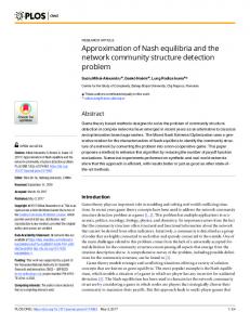
any a priori knowledge about the distribution of the events to be detected and about the detection capabilities of the individual agents. E. Simulations Example 1: In this example we illustrate the algorithm proposed in Fig. 3 for a network of three force-actuated vehicles where the cost functions are given by (61) with
,
,
,
, , , , and . Hence, by solving (41) we obtain that the unique Nash equilibrium . is the point It reflects the compromise between the agents’ “local” objec, and ), and the “collective” tives ( objective of maintaining the network connectivity, deter, mined by the values of the interconnection coefficients ( , ). For the other system parameters we assume the following values: the noise covariance ma, (this trix (6) is phase shift is needed to compensate for the shift obtained in (A.12) is positive definite), in (50) so that the matrix , (washout filters), , , for , and , . We are allowed to pick the same frequencies for the vehicles 1 and 3 since they are not interconnected. The trajectories of the vehicles are shown in Fig. 5, and the coordinates, as a function of time, for the first vehicle are shown in Fig. 6, , , for the initial conditions . The time responses for the other two vehicles are similar. The convergence to the Nash equilibrium while eliminating the measurement noise, is evident. The final minor fluctuations around the equilibrium point are due to the slow convergence of the perturbation amplitudes which are always present as additive inputs. These amplitudes converge to zero much slower than the feedback signals (the outputs of the integrators in Fig. 1) which are additionally . This can also be seen from the definition multiplied by
Fig. 7. Coordinates of the first vehicle: slower convergence rate. The Nash equilibrium is shown as the red line.
of the tracking error (9) which converges to zero faster than the perturbation signal alone. In Fig. 7, a time response for the first agent is depicted for which are the case of slower convergence of the gains , while all the other paramehere ters are kept the same. In this case, the convergence rate to the Nash equilibrium is slower and the algorithm is more sensitive to noise, compared to the responses in Fig. 6. Example 2: In this example, we consider the formation control game, as presented in Section V-D2, performed by three unicycles. Their goal is to reach a formation in which all mutual distances are the same, equal to 1. Therefore, we apply the scheme shown in Fig. 4 with the cost functions given in (61) and with the , , following parameters: , , , and , whose Nash equilibrium corresponds to the formation with all the inter-vehicle distances equal to 1. The other parameters of the scheme , , , are , , , ( ), for , , ,
´ et al.: DISTRIBUTED SEEKING OF NASH EQUILIBRIA WITH APPLICATIONS TO MOBILE SENSOR NETWORKS STANKOVIC
Fig. 8. Trajectories of the unicycles.
917
that their actions are filtered before affecting the measured cost functions. We have formulated conditions on the structure of the game and on the parameters of the proposed scheme, under which we proved almost sure convergence to a Nash equilibrium. It is demonstrated that the proposed method can be applied to networks of mobile robots, where the robots can have single integrator, double integrator or unicycle motion dynamics. We argue that it is desirable and, in some cases, inevitable to use the proposed algorithm for solving problems in mobile sensor networks since these networks usually operate in only partially known or unknown and unpredictable environments with distributed information structure constraints. We give examples of how to formulate problems of connectivity control, formation control, rendezvous, and coverage control as noncooperative games, which can then be directly solved using the proposed framework. The proposed schemes have been illustrated through simulations. As a possible future research direction, one could consider extending the proposed schemes such that they can handle hard-constraints on the actions/positions of the players. In this way, the convergence to a Nash equilibrium could be guaranteed while achieving a collision and/or obstacle avoidance. APPENDIX Proof of Lemma 3: From (12) it follows that . If , is with the transfer the impulse response matrix of the system , we have function matrix
(62) so that Fig. 9. Distances between the unicycles.
(63) and . It is easy to check that all the conditions necessary for applying Theorem 2 are satisfied. Trajectories of the unicycles are shown in Fig. 8, where we have assumed that all the vehicles are initially at the origin. Trajectories are typical for vehicles with rolling without slipping condition (due to nonholonomic constraints) where spikes correspond to the points where a vehicle changes direction of motion. Distances between the vehicles, as functions of time, are shown in Fig. 9. It is evident that all the distances converge to the desired one. The center of the formation depends on the initial conditions and the noise realization. As in the previous example, the small fluctuations after the Nash equilibrium has already been reached, are due , to the slow convergence of the perturbation amplitudes compared to the convergence rate of the tracking error (9).
denotes exponentially decaying terms (due to poswhere sible nonzero initial condition), and can be considered as the output of a time-varying MIMO system with the impulse and input , i.e., response matrix . System is bounded-input, bounded-output (b.i.b.o.) stable, having in mind that all the elare absolutely summable under the formuements of is exponentially stable and satisfies lated assumptions [ (A.2)–(A.5)]. Therefore, since satisis bounded. fies Assumption (A.2) and Proof of Lemma 4: From (14) and the fact that , where is the impulse response matrix of , we obtain
VI. CONCLUSION We have proposed a method for distributive seeking of Nash equilibria in noncooperative games, based only on measurements of the individual cost functions, corrupted by noise. The players are allowed to possess some local linear dynamics, so
(64)
918
IEEE TRANSACTIONS ON AUTOMATIC CONTROL, VOL. 57, NO. 4, APRIL 2012
where denotes exponentially decaying terms (due to possible nonzero initial condition). After iterating (13) times and plugging into the first term in (64), we obtain
. Therefore, due to the boundedness it is easy to derive that , for some uniformly bounded and some constant , . From this it follows that , for some large enough . This proves that the last term in (68) is summable, due to (A.5), which proves the lemma.
for some and of
REFERENCES (65) After regrouping the terms in (65), we obtain (66) where we have incorporated in due to its with exponential decaying. Defining a time varying system , where the impulse response matrix , we can write (67) is the output of when where , which is uniformly bounded by assumption. the input is One can easily verify that is b.i.b.o. stable under the adopted assumptions implying that is uniformly bounded. Theresince fore, we can conclude that satisfies (A.5). Proof of Lemma 5: By denoting , we have that
(68) for some , , where is the integer pe. The first term in the last expression in (68) conriod of verges due to the fact that satisfies (A.2). For the second , for term we will show that . From (15), by using binomial expansion, it some constant follows that
(69)
[1] M. S. Stankovic´, K. H. Johansson, and D. M. Stipanovic´, “Distributed seeking of Nash equilibria in mobile sensor networks,” in Proc. IEEE Conf. Decision Control, 2010, pp. 5598–5603. [2] J. Nash, “Non-cooperative games,” Ann. Math., vol. 54, no. 2, pp. 286–295, 1951. [3] K. Tumer and D. Wolpert, Collectives and the design of complex systems. New York: Springer-Verlag, 2004. [4] D. Monderer and L. S. Shapley, “Potential games,” Games Econ. Behav., no. 14, pp. 124–143, 1996. [5] T. Basar and G. J. Olsder, Dynamic Noncooperative Game Theory, 2nd ed. Philadelphia, PA: SIAM, 1999. [6] P. Dubey, “Inefficiency of Nash equilibria,” Math. Operat. Res., vol. 11, no. 1, pp. 1–8, Feb. 1986. [7] G. Inalhan, D. M. Stipanovic´, and C. J. Tomlin, “Decentralized optimization, with application to multiple aircraft coordination,” in Proc. IEEE Conf. Decision Control, 2002, pp. 1147–1155. [8] L. Buttyan, J.-P. Hubaux, L. Li, X.-Y. Li, T. Roughgarden, and A. Leon-Garcia, “Guest editorial non-cooperative behavior in networking,” IEEE J. Sel. Areas Commun., vol. 25, no. 6, Aug. 2007. [9] T. Roughgarden, “Intrinsic robustness of the price of anarchy,” in Proc. STOC ’09: 41st ACM Symp. Theory of Comput., New York, pp. 513–522. [10] N. Li and J. R. Marden, “Designing games for distributed optimization,” in Proc. IEEE Conf. Decision Control, 2011. [11] S. Li and T. Basar, “Distributed algorithms for the computation of noncooperative equilibria,” Automatica, vol. 23, pp. 523–533, 1987. [12] J. S. Shamma and G. Arslan, “Dynamic fictitious play, dynamic gradient play, and distributed convergence to Nash equilibria,” IEEE Trans. Autom. Control, vol. 50, no. 3, pp. 312–327, Mar. 2005. [13] J. R. Marden, H. P. Young, G. Arslan, and J. S. Shamma, “Payoff based dynamics for multi-player weakly acyclic games,” SIAM J. Control Optim., vol. 48, no. 1, pp. 373–396, 2009. [14] M. Zhu and S. Martinez, “Distributed coverage games for mobile visual sensors (I) : Reaching the set of Nash equilibria,” in Proc. IEEE Conf. Decision Control, 2009, pp. 169–174. [15] H. P. Young, “Learning by trial and error,” Games Econ. Behav., vol. 65, no. 2, pp. 626–643, 2009. [16] M. Krstic, P. Frihauf, J. Krieger, and T. Basar, “Nash equilibrium seeking with finitely- and infinitely-many players,” in Proc. 8th IFAC Symp. Nonlinear Control Syst., 2010. [17] P. Frihauf, M. Krstic, and T. Basar, “Nash equilibrium seeking for dynamic systems with non-quadratic payoffs,” in Proc. 14th Int. Symp. Dynamic Games Applicat., 2010. [18] K. B. Ariyur and M. Krstic, Real Time Optimization by Extremum Seeking. Hoboken, NJ: Wiley, 2003. [19] J. Y. Choi, M. Krstic, K. B. Ariyur, and J. S. Lee, “Extremum seeking control for discrete-time systems,” IEEE Trans. Autom. Control, vol. 47, no. 2, pp. 318–323, Feb. 2002. [20] Y. Tan, D. Neˇsic´, and I. Mareels, “On non-local stability properties of extremum seeking control,” Automatica, vol. 42, pp. 889–903, 2006. [21] M. S. Stankovic´ and D. M. Stipanovic´, “Stochastic extremum seeking with applications to mobile sensor networks,” in Proc. Amer. Control Conf., 2009, pp. 5622–5627. [22] M. S. Stankovic´ and D. M. Stipanovic´, “Extremum seeking under stochastic noise and applications to mobile sensors,” Automatica, vol. 46, pp. 1243–1251, 2010. [23] C. Zhang, A. Siranosian, and M. Krstic, “Extremum seeking for moderately unstable systems and for autonomous vehicle target tracking without position measurements,” Automatica, vol. 43, pp. 1832–1839, 2007. [24] M. S. Stankovic´ and D. M. Stipanovic´, “Discrete time extremum seeking by autonomous vehicles in a stochastic environment,” in Proc. IEEE Conf. Decision Control, 2009, pp. 4541–4546.
´ et al.: DISTRIBUTED SEEKING OF NASH EQUILIBRIA WITH APPLICATIONS TO MOBILE SENSOR NETWORKS STANKOVIC
[25] M. Zavlanos, A. Jadbabaie, and G. Pappas, “Flocking while preserving network connectivity,” in Proc. IEEE Conf. Decision Control, 2007, pp. 2919–2924. [26] M. Schuresko and J. Cortes, “Distributed motion constraints for algebraic connectivity of robotic networks,” J. Intell. Robot. Syst., vol. 56, no. 1–2, pp. 99–126, 2009. [27] D. V. Dimarogonas and K. H. Johansson, “Bounded control of network connectivity in multi-agent systems,” IET Control Theory Applicat., vol. 4, no. 8, pp. 1330–1338, 2010. [28] P. Yang, R. Freeman, G. Gordon, K. Lynch, S. Srinivasa, and R. Sukthankar, “Decentralized estimation and control of graph connectivity for mobile sensor networks,” Automatica, vol. 46, no. 2, pp. 390–396, 2010. [29] M. Mesbahi and M. Egerstedt, Graph Theoretic Methods in Multiagent Networks. Princeton, NJ: Princeton Univ. Press, 2010. [30] R. Olfati-Saber, J. A. Fax, and R. M. Murray, “Consensus and cooperation in networked multi-agent systems,” Proc. IEEE, vol. 95, no. 1, pp. 215–233, Jan. 2007. [31] C. G. Cassandras and W. Li, “Sensor networks and cooperative control,” Eur. J. Control, vol. 11, no. 4–5, pp. 436–463, 2005. [32] J. R. Marden, G. Arslan, and J. S. Shamma, “Cooperative control and potential games,” IEEE Trans. Syst., Man, Cybern. B, vol. 39, no. 6, pp. 1393–1407, Dec. 2009. [33] H.-B. Dürr, M. S. Stankovic´, and K. H. Johansson, “Distributed positioning of autonomous mobile sensors with application to coverage control,” in Proc. Amer. Control Conf., 2011, pp. 4822–4827. [34] H.-B. Dürr, M. S. Stankovic´, and K. H. Johansson, “Nash equilibrium seeking in multi-vehicle systems: A Lie bracket approximation-based approach,” arXiv:1109.6129v2, 2011. [35] G. M. Hoffmann and C. J. Tomlin, “Mobile sensor network control using mutual information methods and particle filters,” IEEE Trans. Autom. Control, vol. 55, no. 1, pp. 32–47, Jan. 2010. [36] A. Ganguli, S. Susca, S. Martinez, F. Bullo, and J. Cortes, “On collective motion in sensor networks: Sample problems and distributed algorithms,” in Proc. IEEE Conf. Decision Control, Dec. 2005, pp. 4239–4244. [37] J. Cortes, S. Martinez, T. Karatas, and F. Bullo, “Coverage control for mobile sensing networks,” IEEE Trans. Robot. Autom., vol. 20, no. 2, pp. 243–255, Apr. 2004. [38] J. Cortes, S. Martinez, and F. Bullo, “Robust rendezvous for mobile autonomous agents via proximity graphs in arbitrary dimensions,” IEEE Trans. Autom. Control, vol. 51, no. 8, pp. 1289–1298, Aug. 2006. [39] B. T. Polyak and Y. Z. Tsypkin, “Pseudogradient algorithms of adaptation and learning,” Autom. Remote Control, no. 3, pp. 45–68, 1973. [40] H. F. Chen, Stochastic Approximation and its Applications. Norwell, MA: Kluwer, 2003. [41] H. J. Kushner and D. S. Clark, Stochastic Approximation Methods for Contrained and Unconstrained Systems. New York: Springer, 1978. [42] L. Ljung, “Analysis of recursive stochastic algorithms,” IEEE Trans. Autom. Control, vol. AC-22, no. 4, pp. 551–575, Aug. 1977. [43] J. B. Rosen, “Existence and uniqueness of equilibrium points for concave n-person games,” Econometrica, vol. 33, no. 3, pp. 520–534, 1965. [44] A. S. Poznyak and D. O. Chikin, “Asymptotic properties of the stochastic approximation procedure with dependent noise,” Autom. Remote Control, no. 12, pp. 78–93, 1984. [45] B. T. Polyak, “Convergence and rate of convergence of iterative stochastic algorithms, II linear case,” Autom. Remote Control, no. 4, pp. 101–107, 1977. [46] B. T. Polyak, “Convergence and rate of convergence of iterative stochastic algorithms, I general case,” Autom. Remote Control, no. 12, pp. 83–94, 1976. [47] C. M. Bishop, Neural Networks for Pattern Recognition. Oxford, U.K.: Clarendon, 1995. [48] C. Zhang, D. Arnold, N. Ghods, A. Siranosian, and M. Krstic, “Source seeking with nonholonomic unicycle without position measurement and with tuning of forward velocity,” Syst. Control Lett., vol. 56, pp. 245–252, 2007. [49] S. S. Stankovic´, M. S. Stankovic´, and D. M. Stipanovic´, “Decentralized parameter estimation by consensus based stochastic approximation,” IEEE Trans. Autom. Control, vol. 56, no. 3, pp. 531–543, Mar. 2011.
919
[50] M. Huang and J. Manton, “Stochastic consensus seeking with noisy and directed inter-agent communication: Fixed and randomly varying topologies,” IEEE Trans. Autom. Control, vol. 55, no. 1, pp. 235–241, Jan. 2010.
Miloˇs S. Stankovic´ received the B.S. and M.S. degrees from the School of Electrical Engineering, University of Belgrade, Belgrade, Serbia, in 2002 and 2006, respectively, and the Ph.D. degree in systems and entrepreneurial engineering from the University of Illinois at Urbana-Champaign (UIUC), in 2009. He was a Research and Teaching Assistant in the Control and Decision Group, Coordinated Science Laboratory, UIUC (2006–2009). In 2009, he joined the Royal Institute of Technology (KTH), Stockholm, Sweden, as a Postdoctoral Researcher in the Automatic Control Laboratory and the ACCESS Linnaeus Centre. His research interests include decentralized control, estimation, detection and system identification, mobile sensor networks, networked control systems, dynamic game theory, optimization, and machine learning.
Karl H. Johansson received the M.Sc. and Ph.D. degrees in electrical engineering from Lund University, Lund, Sweden. He is Director of the ACCESS Linnaeus Centre and Professor at the School of Electrical Engineering, KTH Royal Institute of Technology, Stockholm, Sweden. He has held visiting positions at UC Berkeley (1998–2000) and California Institute of Technology (2006–07). He is a Wallenberg Scholar and has held a Senior Researcher Position with the Swedish Research Council. His research interests are in networked control systems, hybrid and embedded control, and control applications in automotive, automation, and communication systems. Dr. Johansson is the Chair of the IFAC Technical Committee on Networked Systems. He has served on the Executive Committees of several European research projects in the area of networked embedded systems. He is on the editorial board of IET Control Theory and Applications and the International Journal of Robust and Nonlinear Control, and previously of the IEEE TRANSACTIONS ON AUTOMATIC CONTROL and Automatica. He was awarded an Individual Grant for the Advancement of Research Leaders from the Swedish Foundation for Strategic Research in 2005. He received the triennial Young Author Prize from IFAC in 1996 and the Peccei Award from the International Institute of System Analysis, Austria, in 1993. He received Young Researcher Awards from Scania in 1996 and from Ericsson in 1998 and 1999.
Duˇsan M. Stipanovic´ received the B.S. degree in electrical engineering from the University of Belgrade, Belgrade, Serbia, in 1994, and the M.S.E.E. and Ph.D. degrees (under supervision of Prof. ˇ Dragoslav Siljak) in electrical engineering from Santa Clara University, Santa Clara, CA, in 1996 and 2000, respectively. He was an Adjunct Lecturer and Research Associate with the Department of Electrical Engineering, Santa Clara University, from 1998 to 2001, and a Research Associate in Prof. Claire Tomlin’s Hybrid Systems Laboratory, Department of Aeronautics and Astronautics, Stanford University, Stanford, CA, from 2001 to 2004. Since 2004, he has been a faculty member in the Department of Industrial and Enterprise Systems Engineering and Control and Decision Group of the Coordinated Science Laboratory at the University of Illinois at Urbana-Champaign. His research interests include decentralized control and estimation of interconnected systems with application to control of formations of vehicles and sensor networks, stability of discontinuous dynamic systems, differential game theory, and optimization with application to multiple vehicle coordination and systems safety verification.