Download (20Mb) - Warwick WRAP - University of Warwick

University of Warwick institutional repository: http://go.warwick.ac.uk/wrap A Thesis Submitted for the Degree of PhD at the University of Warwick http://go.warwick.ac.uk/wrap/67156 This thesis is made available online and is protected by original copyright. Please scroll down to view the document itself. Please refer to the repository record for this item for information to help you to cite it. Our policy information is available from the repository home page.

A Study of Point Defects in CVD Diamond Using Electron Paramagnetic Resonance and Optical Spectroscopy by

Christopher Brett Hartland Thesis Submitted to The University of Warwick for the degree of

Doctor of Philosophy

Department of Physics August 2014

Contents List of Figures

vi

List of Tables

ix

Acknowledgements

xi

Declaration of Authorship

xiii

Abstract

xvi

Abbreviations

xvii

1 Introduction 1.1 An early history of diamond . . . . . . . 1.2 The structure and properties of diamond 1.3 Defects and impurities in diamond . . . 1.4 Synthetic diamond . . . . . . . . . . . . 1.5 Applications of diamond . . . . . . . . . 1.6 Motivation for study . . . . . . . . . . . 1.7 Thesis outline . . . . . . . . . . . . . . .

. . . . . . .

. . . . . . .

. . . . . . .

. . . . . . .

. . . . . . .

. . . . . . .

. . . . . . .

. . . . . . .

. . . . . . .

2 Literature review 2.1 Growth methods . . . . . . . . . . . . . . . . . . . . . . 2.1.1 HPHT diamond synthesis . . . . . . . . . . . . . 2.1.1.1 Defect incorporation in HPHT diamond 2.1.2 CVD diamond synthesis . . . . . . . . . . . . . . 2.1.2.1 Defect incorporation in CVD diamond . 2.2 Irradiation of diamond . . . . . . . . . . . . . . . . . . . 2.2.1 Irradiation damage in type IIa diamond . . . . . 2.2.2 Irradiation of type Ib diamonds . . . . . . . . . . 2.3 Other literature reviews through this thesis . . . . . . . .

. . . . . . .

. . . . . . . . .

. . . . . . .

. . . . . . . . .

. . . . . . .

. . . . . . . . .

. . . . . . .

. . . . . . . . .

. . . . . . .

. . . . . . . . .

. . . . . . .

1 1 2 4 5 6 8 9

. . . . . . . . .

11 11 12 13 14 16 20 21 22 24

3 Theory 25 3.1 Electron paramagnetic resonance . . . . . . . . . . . . . . . . . . . 25 ii

Contents

iii

3.1.1 3.1.2 3.1.3

3.2

3.3 3.4 3.5 3.6

Electron magnetic dipole moment . . . . . . . . . . Resonance conditions . . . . . . . . . . . . . . . . . The spin Hamiltonian . . . . . . . . . . . . . . . . 3.1.3.1 Electronic Zeeman interaction . . . . . . . 3.1.3.2 Zero-field interaction . . . . . . . . . . . . 3.1.3.3 Hyperfine interaction . . . . . . . . . . . . 3.1.3.4 Nuclear Zeeman interaction . . . . . . . . 3.1.3.5 Quadrupole interaction . . . . . . . . . . . 3.1.4 Transition probabilities . . . . . . . . . . . . . . . . 3.1.5 Spin relaxation and the Bloch absorption lineshape Optical absorption . . . . . . . . . . . . . . . . . . . . . . 3.2.1 Transition probability . . . . . . . . . . . . . . . . 3.2.2 Electronic and vibronic transitions . . . . . . . . . 3.2.3 Vibrational transitions . . . . . . . . . . . . . . . . 3.2.4 Isotope effects on local vibrational modes . . . . . . Point defect photo-luminescence . . . . . . . . . . . . . . . Symmetry . . . . . . . . . . . . . . . . . . . . . . . . . . . Electronic configuration of the vacancy in diamond . . . . The effect of dynamic reorientation on EPR spectra . . . .

4 Experimental details 4.1 EPR . . . . . . . . . . . . . . . . . . . . . . . . . 4.1.1 The static magnetic field . . . . . . . . . . 4.1.2 Microwave source and bridge . . . . . . . . 4.1.3 Resonant cavities . . . . . . . . . . . . . . 4.1.4 Detection . . . . . . . . . . . . . . . . . . 4.1.5 EPR spectrometers and sample mounting . 4.1.6 Quantitative EPR . . . . . . . . . . . . . . 4.1.7 Low-temperature measurements . . . . . . 4.1.8 In-situ optically illuminated EPR . . . . . 4.1.9 Simulation and fitting . . . . . . . . . . . 4.2 Optical spectroscopy . . . . . . . . . . . . . . . . 4.2.1 UV-Vis absorption spectroscopy . . . . . . 4.2.2 Photo-luminescence spectroscopy . . . . . 4.2.3 Infra-red absorption spectroscopy . . . . . 4.3 Treatment processes . . . . . . . . . . . . . . . . 4.3.1 Electron irradiation . . . . . . . . . . . . . 4.3.2 Annealing . . . . . . . . . . . . . . . . . . 4.3.3 Charge transfer . . . . . . . . . . . . . . . 4.3.4 Annealing kinetics . . . . . . . . . . . . . 4.3.4.1 First order kinetics . . . . . . . . 4.3.4.2 Second order kinetics . . . . . . .

. . . . . . . . . . . . . . . . . . . . .

. . . . . . . . . . . . . . . . . . . . .

. . . . . . . . . . . . . . . . . . . . .

. . . . . . . . . . . . . . . . . . . . .

. . . . . . . . . . . . . . . . . . . . .

5 Identification of the di-nitrogen-vacancy-hydrogen centre

. . . . . . . . . . . . . . . . . . .

. . . . . . . . . . . . . . . . . . . . .

. . . . . . . . . . . . . . . . . . .

. . . . . . . . . . . . . . . . . . . . .

. . . . . . . . . . . . . . . . . . .

. . . . . . . . . . . . . . . . . . . . .

. . . . . . . . . . . . . . . . . . .

. . . . . . . . . . . . . . . . . . . . .

. . . . . . . . . . . . . . . . . . .

26 27 28 29 31 33 36 36 37 38 41 41 42 45 47 48 49 52 53

. . . . . . . . . . . . . . . . . . . . .

58 58 58 59 61 64 65 66 68 69 70 72 72 74 74 75 75 76 77 78 79 80 82

Contents 5.1

5.2 5.3 5.4

5.5

Introduction . . . . . . . . . . . . . . 5.1.1 The NVH centre in diamond . 5.1.2 The N3 VH centre in diamond Experimental details . . . . . . . . . Results . . . . . . . . . . . . . . . . . Discussion . . . . . . . . . . . . . . . 5.4.1 15 N2 VH0 . . . . . . . . . . . . 5.4.2 Reorientation of N2 VH0 . . . Conclusions . . . . . . . . . . . . . .

iv . . . . . . . . .

. . . . . . . . .

. . . . . . . . .

. . . . . . . . .

. . . . . . . . .

. . . . . . . . .

. . . . . . . . .

. . . . . . . . .

. . . . . . . . .

. . . . . . . . .

. . . . . . . . .

. . . . . . . . .

. . . . . . . . .

. . . . . . . . .

. . . . . . . . .

6 Production and properties of the N2 VH0 and N3 VH0 centres 6.1 Introduction . . . . . . . . . . . . . . . . . . . . . . . . . . . . . 6.1.1 Nitrogen aggregation in natural and HPHT diamond . . 6.1.2 Models for the aggregation process . . . . . . . . . . . . 6.1.3 Annealing of defects in CVD diamond . . . . . . . . . . 6.2 Experimental details . . . . . . . . . . . . . . . . . . . . . . . . 6.3 Results . . . . . . . . . . . . . . . . . . . . . . . . . . . . . . . . 6.3.1 Isochronal annealing of GC2 . . . . . . . . . . . . . . . . 6.3.2 Study of samples with high N2 VH0 concentrations . . . . 6.3.2.1 EPR . . . . . . . . . . . . . . . . . . . . . . . . 6.3.2.2 Optical absorption . . . . . . . . . . . . . . . . 6.4 Discussion . . . . . . . . . . . . . . . . . . . . . . . . . . . . . . 6.4.1 Analysis of features observed by optical techniques . . . 6.4.2 Charge transfer of N2 VH0 . . . . . . . . . . . . . . . . . 6.4.3 Optical analogue for N2 VH0 . . . . . . . . . . . . . . . . 6.4.4 Aggregation processes in CVD diamond . . . . . . . . . 6.5 Conclusions and further work . . . . . . . . . . . . . . . . . . .

. . . . . . . . .

. . . . . . . . .

. . . . . . . . . . . . . . . .

111 . 111 . 111 . 114 . 116 . 118 . 121 . 121 . 130 . 130 . 132 . 137 . 137 . 138 . 139 . 141 . 144

7 Oxygen defects in diamond 7.1 Introduction . . . . . . . . . . . . . . . . . . . . . . . . . . . . . . 7.1.1 Challenges in the study of oxygen by EPR . . . . . . . . . 7.1.2 The neutral oxygen-vacancy centre . . . . . . . . . . . . . 7.1.3 13 C analysis for NV- and Os V0 . . . . . . . . . . . . . . . . 7.1.3.1 Spin polarisation of NV- and Os V0 . . . . . . . . 7.1.3.2 Production and annealing behaviour of the NVand Os V0 centres . . . . . . . . . . . . . . . . . . 7.1.4 Oxygen in silicon . . . . . . . . . . . . . . . . . . . . . . . 7.1.5 The neutral oxygen-vacancy-hydrogen defect in diamond . 7.2 Experimental details . . . . . . . . . . . . . . . . . . . . . . . . . 7.3 Results . . . . . . . . . . . . . . . . . . . . . . . . . . . . . . . . . 7.3.1 Annealing study . . . . . . . . . . . . . . . . . . . . . . . . 7.3.2 Irradiation and annealing . . . . . . . . . . . . . . . . . . 7.3.3 Spin polarisation . . . . . . . . . . . . . . . . . . . . . . . 7.3.4 Observation of previously unreported EPR signal in CVD diamond . . . . . . . . . . . . . . . . . . . . . . . . . . . .

82 85 87 88 89 93 104 106 109

146 . 146 . 146 . 147 . 149 . 150 . . . . . . . .

152 153 154 157 159 159 160 161

. 162

Contents 7.4

7.5

Discussion . . . . . . . . . . . . . . . . . . . . . . . . . . . . . . . 7.4.1 Annealing study . . . . . . . . . . . . . . . . . . . . . . . . 7.4.2 Irradiation and annealing study . . . . . . . . . . . . . . . 7.4.3 Spin polarisation . . . . . . . . . . . . . . . . . . . . . . . 7.4.4 Observation of a previously unreported EPR signal in CVD diamond . . . . . . . . . . . . . . . . . . . . . . . . . . . . Conclusions and further work . . . . . . . . . . . . . . . . . . . .

v . . . .

162 162 164 166

. 167 . 174

8 Effects of irradiation and annealing on as-grown and annealed CVD diamond 177 8.1 Introduction . . . . . . . . . . . . . . . . . . . . . . . . . . . . . . . 177 8.1.1 The Ns :H–C0 defect . . . . . . . . . . . . . . . . . . . . . . . 177 8.1.2 The Vn H- defect . . . . . . . . . . . . . . . . . . . . . . . . 178 8.1.3 Hydrogen interstitials in diamond . . . . . . . . . . . . . . . 180 8.2 Experimental details . . . . . . . . . . . . . . . . . . . . . . . . . . 182 8.3 Results . . . . . . . . . . . . . . . . . . . . . . . . . . . . . . . . . . 184 8.3.1 Irradiation and annealing of as-grown CVD diamond . . . . 184 8.3.2 Triple treatment of CVD diamond . . . . . . . . . . . . . . . 192 8.4 Discussion . . . . . . . . . . . . . . . . . . . . . . . . . . . . . . . . 195 8.4.1 Reintroduction of Vn H- . . . . . . . . . . . . . . . . . . . . . 195 8.4.2 Production of the 3324 cm-1 LVM . . . . . . . . . . . . . . . 197 8.4.3 Plateau of NV concentration . . . . . . . . . . . . . . . . . . 198 8.4.4 NV concentration variation under irradiation and annealing treatments . . . . . . . . . . . . . . . . . . . . . . . . . . . . 200 8.5 Conclusions . . . . . . . . . . . . . . . . . . . . . . . . . . . . . . . 202 8.6 Further work . . . . . . . . . . . . . . . . . . . . . . . . . . . . . . 203 9 Summary and further work 9.1 Introduction . . . . . . . . . . . . . . . . . . . . . . . . . . . . . . 9.2 Identification of the neutral di-nitrogen-vacancy-hydrogen centre . 9.3 Production and properties of the N2 VH0 and N3 VH0 centres . . . . 9.4 Oxygen defects in diamond . . . . . . . . . . . . . . . . . . . . . . 9.5 Effects of irradiation and annealing on as-grown and annealed CVD diamond . . . . . . . . . . . . . . . . . . . . . . . . . . . . . . . .

Bibliography

205 . 205 . 206 . 206 . 208 . 209

211

List of Figures 1.1 1.2

The diamond unit cell . . . . . . . . . . . . . . . . . . . . . . . . . Classification scheme of diamond. . . . . . . . . . . . . . . . . . . .

2.1 2.2

The phase diagram of carbon . . . . . . . . . . . . . . . . . . . . . 12 A simplified depiction of the C:H:O phase diagram for CVD growth 15

3.1

The precession of magnetic moments in under the influence of an external magnetic field. . . . . . . . . . . . . . . . . . . . . . . . . Example configuration co-ordinate diagram showing zero-phonon and vibronic transitions . . . . . . . . . . . . . . . . . . . . . . . Simulations of the Ns 0 used to show the effect of changing the external magnetic field direction with respect to the crystal lattice . Demonstration of the effect that defect reorientation can have on an EPR spectrum . . . . . . . . . . . . . . . . . . . . . . . . . . .

3.2 3.3 3.4 4.1 4.2 4.3 4.4 4.5 4.6 4.7 4.8 4.9 5.1 5.2 5.3 5.4 5.5 5.6

The set up for a typical continuous wave EPR spectrometer. . . . A TE011 cylindrical resonator. . . . . . . . . . . . . . . . . . . . . The effect of modulation on the EPR signal lineshape . . . . . . . A schematic diagram of the Oxford Instruments ESR-900 continuous flow cryostat. . . . . . . . . . . . . . . . . . . . . . . . . . . . A schematic diagram of the experimental set up for the 1 kW arc lamp system and associated optics. . . . . . . . . . . . . . . . . . A screenshot of the EPRsimulator program. . . . . . . . . . . . . A diagram of the Perkin-Elmer Lambda 1050 UV-Vis absorption spectrometer. . . . . . . . . . . . . . . . . . . . . . . . . . . . . . A room temperature experimental IR spectrum of a IIa diamond. The charge transfer mechanism in diamond . . . . . . . . . . . . .

. 40 . 43 . 50 . 55 . 59 . 62 . 64 . 69 . 70 . 71 . 72 . 75 . 79

The energy levels which are available for defects with four atomic orbitals with Td , C3v or C2v symmetry. . . . . . . . . . . . . . . . . Model for the NVH- centre . . . . . . . . . . . . . . . . . . . . . . . Structural and electronic model for the N3 V and N3 VH0 defects. . . EPR spectrum of sample HE1 showing previously unreported WAR13 defect at X- and Q-band frequencies. . . . . . . . . . . . . . . . . . Q-band spectrum of WAR13 highlighting the forbidden transitions. Energy level diagram showing the origin of the electron-proton double spin flip transitions. . . . . . . . . . . . . . . . . . . . . . . . . . vi

2 4

83 87 88 91 92 93

List of Figures 5.7 5.8 5.9 5.10 5.11

5.12 5.13 5.14 5.15 5.16 6.1 6.2 6.3 6.4 6.5 6.6 6.7 6.8 6.9 6.10 6.11 6.12 6.13 6.14 6.15 7.1 7.2 7.3 7.4 7.5

vii

X-band fit of N2 VH0 to WAR13 signal. . . . . . . . . . . . . . . . . 96 Q-band fit of N2 VH0 to WAR13 signal. . . . . . . . . . . . . . . . . 97 Q-band roadmap showing the fit of N2 VH0 to the WAR13 signal. . 98 Figure showing the tilt of the nitrogen hyperfine interactions in N2 VH0 . . . . . . . . . . . . . . . . . . . . . . . . . . . . . . . . . . 100 A depiction of the N2 VH0 centre showing how the hydrogen can be considered as a bond-centred interstitial hydrogen between two carbon atoms. . . . . . . . . . . . . . . . . . . . . . . . . . . . . . . 102 15 N2 VH0 simulation fit to experimental data with B0 parllel to 〈001〉.104 15 N2 VH0 simulation fit to experimental data with B0 parllel to 〈110〉.105 15 N2 VH0 simulation fit to experimental data with B0 parllel to 〈111〉.105 An outline of the 〈110〉sites and directions for rhombic and monoclinic defects. . . . . . . . . . . . . . . . . . . . . . . . . . . . . . . 107 Demonstration of the effect of reorientation on N2 VH0 EPR spectrum.108 The percentage of nitrogen aggregation for a range of temperatures as a function of starting Ns 0 concentration. . . . . . . . . . . . . . . Example of concerted exchange between a nitrogen and a vacancy. . Example of Ns + fit. . . . . . . . . . . . . . . . . . . . . . . . . . . . Infra-red spectra of the isochronal annealing study on sample GC2. Variation of Ns , NVH, N2 VH0 and N3 VH0 concentrations through isochronal annealing study on sample GC2. . . . . . . . . . . . . . . UV-Vis and PL spectra recorded for the isochronal annealing study of sample GC2. . . . . . . . . . . . . . . . . . . . . . . . . . . . . . DiamondView images of sample GC2 at each stage of its isochronal annealing study. . . . . . . . . . . . . . . . . . . . . . . . . . . . . . An example of the quality of fit which can be achieved when multiple overlapping spin systems are present in the sample. . . . . . . . . . Ex-situ isochronal annealing of Ns 0 and N2 VH0 results. . . . . . . . In-situ isochronal annealing of N2 VH0 results. . . . . . . . . . . . . Isochronal IR charge transfer results from sample JE1. . . . . . . . IR spectra of samples with high N2 VH0 concentrations. . . . . . . . UV-Vis spectra of samples containing high N2 VH0 concentrations. . Plot of 1378 cm-1 against N2 VH0 concentration. . . . . . . . . . . . Example fit of A-centres to an experimental IR spectrum of sample JB1. . . . . . . . . . . . . . . . . . . . . . . . . . . . . . . . . . . . Mechanism of spin polarisation for NV- . . . . . . . . . . . . . . . A model of the V(OH) defect. . . . . . . . . . . . . . . . . . . . . Annealing behaviour of the Os V0 and NV defects as calculated by EPR and UV-Vis absorption, respectively. . . . . . . . . . . . . . The result of irradiation and annealing on NV and Os V0 concentrations. . . . . . . . . . . . . . . . . . . . . . . . . . . . . . . . . . . Example of the quality of fit obtainable for NVH and Ns 0 in a sample containing only these defects compared to a fit for these two defects in a sample studied in this thesis. . . . . . . . . . . . . . . . . . .

113 115 120 122 125 126 129 130 131 131 133 134 136 139 143

. 150 . 155 . 160 . 161

. 163

List of Figures 7.6

7.7

7.8 7.9

Experimental spectra shown alongside simulations with the Os VH0 simulation to show the improvement this makes to the overall fit. Magnetic field along 〈001〉. . . . . . . . . . . . . . . . . . . . . . . . . . 169 Experimental spectra of the electron-proton double spin flips shown alongside simulations with and without the Os VH0 simulation to show the improvement this makes to the overall fit. Magnetic field along 〈001〉. . . . . . . . . . . . . . . . . . . . . . . . . . . . . . . . 170 The model for the Os VH0 defect presented in this Chapter. . . . . . 171 Experimental spectra shown alongside simulations with and without the Os VH0 simulation to show the improvement this makes to the overall fit. Magnetic field along 〈111〉. . . . . . . . . . . . . . . . . . 172

The model of the Ns :H–C0 defect. . . . . . . . . . . . . . . . . . . The two possible models of the Vn H- defect. . . . . . . . . . . . . Four possible configurations for the hydrogen interstitial. . . . . . Vacancy and interstitial production plotted against irradiation time for samples studied in Chapters 7 and 8. . . . . . . . . . . . . . . 8.5 The UV-Vis absorption spectra for sample GC3 after each treatment stage. . . . . . . . . . . . . . . . . . . . . . . . . . . . . . . 8.6 The total NV concentration in each sample after each irradiation and anneal to 800 ◦ C plotted against number of vacancies produced in the sample after irradiation. . . . . . . . . . . . . . . . . . . . . 8.7 FTIR measurements for sample GC3 after each treatment stage. . 8.8 Irradiation duration is plotted against 3324 cm-1 integrated intensity showing a linear relationship between these. . . . . . . . . . . 8.9 FTIR spectra of sample GG1 taken after heat treatment at each treatment stage. . . . . . . . . . . . . . . . . . . . . . . . . . . . . 8.10 Correlation of the loss of NVH from the initial concentration in each sample against the integrated intensity of the 3324 cm-1 LVM. . . 8.11 Concentration variations of Ns , NV and N2I showing that the total nitrogen concentration can be accounted for by these defects. . . .

8.1 8.2 8.3 8.4

viii

. 178 . 180 . 181 . 185 . 186

. 188 . 189 . 192 . 193 . 197 . 201

List of Tables 1.1 3.1 3.2

Selected properties of diamond compared to a number of other semiconductor materials. . . . . . . . . . . . . . . . . . . . . . . . . . .

3

Natural abundances, nuclear spins and 100% localisation hyperfine parameters for common elements in CVD diamond . . . . . . . . . 36 The possible symmetries which can exist in a lattice with Td symmetry. . . . . . . . . . . . . . . . . . . . . . . . . . . . . . . . . . . 57

4.1 4.2 4.3

Commonly used EPR frequencies . . . . . . . . . . . . . . . . . . . 60 Descriptions of the resonators used throughout this thesis. . . . . . 63 Optical absorption coefficients which have been used to calculate defect concentrations throughout this thesis. . . . . . . . . . . . . . 81

5.1 5.2

Sample details for Chapter 5. . . . . . . . . . . . . . . . . . . . . . Final Hamiltonian parameters for the fit of the WAR13 signal to the N2 VH0 defect. . . . . . . . . . . . . . . . . . . . . . . . . . . . . Comparison of the 14 N quadrupole parameters for four Nn V and Nn VH defects where n = 1 − 2 in this case. . . . . . . . . . . . . . . Hamiltonian parameters for the N2 V as determined by B.L. Green.

5.3 5.4 6.1 6.2 6.3 6.4 6.5 7.1 7.2 7.3 7.4 8.1

90 94 103 106

Rate constants for the aggregation of nitrogen into A-centres. . . . 112 Sample data for Chapter 6. . . . . . . . . . . . . . . . . . . . . . . 118 Annealing behaviour of defects observed by IR absorption in isochronal annealing study on sample GC2. . . . . . . . . . . . . . . . . . . . . 123 Concentrations of common defects in CVD diamond for the samples studied in Chapter 6. . . . . . . . . . . . . . . . . . . . . . . . . . . 127 Comparison of the rate of aggregation in CVD diamond against that predicted by the rate constants of Evans and Qi. . . . . . . . . 140 Binding energies for charged and uncharged Os V and NV complexes.153 Spin Hamiltonian parameters for the V(OH) defect proposed by Komarovskikh. . . . . . . . . . . . . . . . . . . . . . . . . . . . . . 155 Treatment details for samples studied in Chapter 7. . . . . . . . . . 157 Comparison of the motionally averaged and static Os VH0 spin Hamiltonian parameters used in the fits throughout Chapter 7. . . . . . . 173 Sample details for those used in Chapter 8. . . . . . . . . . . . . . . 182

ix

List of Tables 8.2 8.3 8.4 8.5

As-grown concentrations of quantifiable defects in samples studied in Chapter 8. . . . . . . . . . . . . . . . . . . . . . . . . . . . . . The behaviour of features observed by UV-Vis absorption in sample GC3 over the course of an irradiation and annealing study. . . . . The behaviour of features observed by FTIR in sample GC3 over the course of an irradiation and annealing study. . . . . . . . . . . Concentration variation of defects in sample GG1 after each treatment stage. . . . . . . . . . . . . . . . . . . . . . . . . . . . . . .

x

. 183 . 187 . 191 . 194

Acknowledgements I owe my most profound thanks to Professor Mark Newton for his guidance, support and patience throughout the course of my PhD. I would also like to thank Dr. Chris Welbourn for his advice and assistance over the last four years. To Professor Michael Baker I must extend my gratitude for many interesting discussions and his continual interest in my research. To Dr. Jon Goss I will always be thankful for our varied conversations (both about diamond and broader subjects!), the invaluable opinion of a theoretician and the lunches I was treated to on my visits to Newcastle. I would like to thank the team at De Beers Technologies, Maidenhead, for financial and technical support over the years. In particular I thank Dr. Riz Khan who has been both supervisor and a friend over the years, Dr. Brad Cann for his patience for my endless stream of e-mails, to Dr. Philip Martineau, Dr. David Fisher and the rest of the team at Maidenhead. I also extend my thanks to the whole team at Element Six including Dr. Jacqueline Hall for going out of her way to get an anneal completed in time for incorporation into my thesis. I cannot thank the other Warwick EPR & Diamond Group students, past and present, enough for their support, but I will try. My greatest thanks to: Stephanie for the best advice I have received; Andy, for revealing the magic in his programs; Ulrika, for training me; Ben G for his invaluable help and irreplaceable friendship; Matthew, for not begrudging me stealing his spectrometer time (too much); Mika, for all of the cookies and his positive attitude; Ben B, for always believing my signals weren’t noise; Anton, for convincing me that Apple is the way to go and not judging me too much when I still bought other products; Claudio, for always making me smile no matter what was happening; Sinead, for taking on all of the contract work I am leaving behind; and Angelo, for helping me to see the other side of any debate. To my veritable army of proof readers I must extend my thanks. Those not already thanked include: Daniel, Mark L, Dave, Tom, Ian, Chris E, Josh and Patrick. Over the years you have all been the best kinds of friends a man can ask for and I appreciate everything you have done for me, thesis related and beyond. To Elena, my partner in all things: I could not have finished my PhD studies without you. You have provided me with the love, support and friendship. You xi

List of Tables

xii

have been patient and kind and have always given me the right advice. You have cooked for me, cared for me and helped me to get my dream job. I love you more than you can know. Finally my thanks to my Mum, Dad and Brother. I would not be here without your support. You are always there for me through every trial and tribulation. I would not have made it out of high school without your guidance and I certainly would not have made it to the end of a PhD without your love. The phrase “Diamonds are forever” is a lie, they degrade eventually, they can be sundered or they can be burnt. Family, however, that is forever. It is to my family that I dedicate this thesis.

Declaration of Authorship I, Christopher Brett Hartland, declare that the work presented in this thesis is my own except where stated otherwise, and was carried out entirely at the University of Warwick during the period of October 2010 to August 2014 under the supervision of Prof. M. E. Newton. The research reported here has not been submitted, either wholly or in part, in this or any other academic institution, for admission to a higher degree.

Published papers [ 1 ] Khan, R. U. A., Cann, B. L., Martineau, P. M., Samartseva, J., Freeth, J. J. P., Sibley, S. J., Hartland, C. B., Newton, M. E., Dhillon, H. K., and Twitchen, D. J. Journal of physics. Condensed Matter: Condensed Matter 25(27), 275801 (2013)

Conference presentations [ 1 ] Hartland, C. B., Green, B. L., Welbourn, W. and Newton, M. E., Irradiation damage defects in type IIb diamond (2011), poster presentation at the 62nd Diamond Conference (Coventry, UK) [ 2 ] Hartland, C. B. and Newton, M. E., An investigation of the point defects produced in multiply treated CVD diamond (2012), poster presentation at the 63rd Diamond Conference (Coventry, UK) [ 3 ] Dale, M. W., Green, B. L., Hartland, C. B. and Newton, M. E., Quantitative electron paramagnetic resonance measurements on defects in diamond: challenges and solutions (2012), poster presentation at the 63rd Diamond Conference (Coventry, UK) [ 4 ] Hartland, C. B., Newton, M. E., Cann, B. L., Khan, R. U. A., Twitchen, D. J., Dhillon, H., Electron paramagnetic resonance studies on oxygen doped CVD diamond (2013), poster presentation at the 18th Hasselt diamond workshop (Hasselt, Belgium) xiii

List of Tables

xiv

[ 5 ] Hartland, C. B., Newton, M. E., Cann, B. L., Khan, R. U. A., Twitchen, D. J., Dhillon, H., Electron paramagnetic resonance studies on oxygen doped CVD diamond (2013), oral presentation at 46th annual international meeting of the ESR spectroscopy group of the Royal Society of Chemistry (Coventry, UK) [ 6 ] Hartland, C. B., Green, B. L., Newton, M. E., Khan, R. U. A., Cann, B. L., Identification of the neutral di-nitrogen-vacancy-hydrogen defect in diamond (2013), oral presentation at 64th Diamond Conference (Coventry, UK)

Signed:

Date:

“Better a diamond with a flaw than a pebble without.”

Confucius

Abstract A Study of Point Defects in CVD Diamond Using Electron Paramagnetic Resonance and Optical Spectroscopy This thesis reports research on the characterisation of the structure of point defects in chemical vapour deposition (CVD) diamond. Electron paramagnetic resonance (EPR) has been used as a tool to determine the constituent nuclei and symmetry of previously unreported EPR active defects. Optical spectroscopy has been employed to track defect concentrations and correlate optical features with EPR active defects. Multi-frequency EPR has been used to identify and characterise a previously unreported EPR signal arising from N2 VH0 : a vacancy bounded by two substitutional nitrogen atoms and two carbon atoms wherein a hydrogen is bonded along one of the two carbon atoms and the unpaired electron of the system is bonded along the second carbon. This defect exhibits C2v symmetry in both X- and Q-band EPR, suggesting that the hydrogen rapidly reorientates between the two equivalent carbon atoms resulting in a time averaged C2v symmetry. The effects of annealing CVD diamond have been investigated. It has been shown that N2 VH0 is produced consistently upon annealing at 1800 ◦ C and continues to increase in intensity up to 2200 ◦ C. The charge transfer behaviour of the N2 VH0 defect is reported and the local vibrational mode (LVM) doublet at 1375 and 1378 cm-1 has been correlated with the intensity of the N2 VH0 EPR signal. A calibration coefficient for the concentration of N3 VH0 as calculated from the integrated intensity of the 3107 cm-1 LVM is proposed and a nitrogen assay of six samples in the as-grown and post-treated states suggest that this is a reasonable estimate. The annealing behaviour of the WAR5 EPR centre has been investigated and found to match density functional theory (DFT) predictions for the binding energy of the Os V defect. It has been reported that the WAR5 signal can be increased in intensity upon the irradiation and annealing at 800 ◦ C of CVD diamond grown from a C:H:O chemistry, further supporting the assignment of this signal to the OV0 defect. A new EPR signal is reported and characterised as arising from a substitutional oxygen adjacent to a vacancy wherein a hydrogen atom rapidly reorientates between the three available carbon dangling bonds (Os VH0 ). The effect of irradiation and annealing on as-grown and pre-annealed CVD diamond has been investigated. It is shown that the 3324 cm-1 LVM (arising from the Ns :H–C0 defect) can be introduced into CVD diamond upon irradiation and further increased in intensity by annealing at 600 ◦ C. The increase in 3324 cm-1 intensity has been correlated with a loss of NVH allowing a calibration correlation for this centre to be determined. Further, the reintroduction of the Vn H- defect has been reported in a diamond sample which has been annealed prior to additional irradiation and annealing treatments.

Abbreviations CVD

Chemical Vapour Deposition

DFT

Density Functional Theory

EM

Electro Magnetic

EPR

Electron Paramagnetic Resonance

FTIR

Fourier Transform Infra Red

HPHT

High Pressure High Temperature

LVM

Local Vibrational Mode

NMR

Nuclear Magnetic Resonance

PL

Photo Luminescence

ppb

parts per billion

ppm

parts per million

UV-Vis

Ultra Violet Visible

ZPL

Zero Phonon Line

xvii

Chapter 1 Introduction

1.1

An early history of diamond

The word diamond derives from the Greek adamas which translates as ‘unconquerable’ or ‘invincible’, it is perhaps for the hope that this characteristic would be conferred upon the bearer that diamonds became highly desirable by the rich and powerful [1]. One of the first references to diamond being used as a tool is found in the Bible in which Jeremiah writes “The sin of Judah is written with a pen of iron and with the point of a diamond. It is graven upon the table of their heart and upon the horns of your altar.”(Jeremiah 17:1, The Bible). Since these times diamond has developed significantly as both a decorative item and as a tool for technological applications. As the cutting and polishing of diamond was developed it was discovered that these stones could be made into items of great beauty. Diamonds then started being worn by women in the form of jewellery. The first diamond engagement ring was presented to Mary of Burgundy by the Archduke Maximillian of Austria in 1477 [2]. Despite this, diamond engagement rings were not widely used until the 1930’s when De Beers began their famously successful marketing campaign. “A diamond is forever” was the slogan used by De Beers in their marketing campaign which led 1

Chapter 1. Introduction

2

to 90 % of engagement rings now bearing at least one diamond [2]. The revenues from rough diamond sales in the year 2012 – 2013 were recorded at $14.8 billion worldwide whilst the retail sales for diamond jewellery reached $72.1 billion [3]. Natural diamond is marketed as a piece of the earth’s history where that symbol of eternity is used as a symbol of eternal love in the gift of a diamond ring. This marketing strategy has led to consumer demand for natural stones as opposed to synthetic ones. Synthetic diamonds will be discussed later in this chapter and in further detail in Chapter 2.

1.2

The structure and properties of diamond

Diamond is a metastable allotrope of carbon. Carbon is a chemical element comprised of six protons, six electrons and, in its most naturally abundant form, six neutrons. The electronic configuration of carbon in its ground state is 1s2 2s2 2p2 , however, in order to form diamond an electron from the 2s level is instead localised in a 2p orbital thereby allowing for covalent bonds to be formed with four neighbouring carbon atoms in a tetrahedral geometry by sp3 hybridisation [5]. sp2

1 1 1 , , 4 4 4

(0, 0, 0)

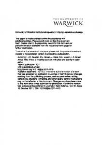
a0 = 0.357 nm Figure 1.1: The diamond unit cell with side of length a0 = 0.357 nm. A single tetrahedral unit has been highlighted with darker spheres. Variations of this figure will be used to demonstrate the structure of the point defects presented throughout this thesis. Adapted from [4].


3 Si

Bandgap (eV) Breakdown field (MVm-1 ) Electron mobility (cm2 V-1 s-1 ) Hole mobility (cm2 V-1 s-1 ) Thermal conductivity (W m-1 K-1 )

SiC

GaN

Diamond

1.1 3.2 30 300 1450 900 480 120 150 500

3.44 500 440 200 130

5.47 2000 4500 3800 2400

Table 1.1: Selected properties of diamond compared to a number of other semiconductor materials. Adapted from [7].

hybridisation leads to the formation of graphite which is the stable form of carbon. Graphite has three bonds to neighbouring atoms while the final electron forms a weakly bonded π-orbital. The tetrahedral units formed by the bonding of the carbon atoms results in a structure comprised of two inter-penetrating face-centred cubic (fcc) lattices where one sublattice is displaced by a0 /4. This structure is shown in Figure 1.1. The short bond lengths in diamond result in it having an atomic density of 1.76 × 1023 cm-3 , the highest of any 3D solid [6]. Diamond has a wide variety of extreme properties which are a result of its bonding configuration, some of these are presented in Table 1.1 along with comparisons to other semi-conductor materials. The hardness of the material is such that it is used as the maximum point of the Mohs hardness scale [8]. Diamond is chemically and biologically inert and also radiation hard. This makes it ideal for use in a range of extreme environments in which other materials would not be suitable. The strong covalent bonds and low phonon scattering in diamond also makes it an excellent thermal conductor with a conductivity five times greater than that of copper at room temperature. The band gap of intrinsic diamond is significantly greater than that of other common semi-conductor materials, as shown in Table 1.1. The broad optical window which results from the wide band-gap and the very high phonon propagation frequency of diamond makes it an ideal material for use as an optical window from 227 nm through to 2.5 µm [9].


4 Diamond

Type I Nitrogen content > ∼ 1-2 ppm

Type Ia Nitrogen in aggregated form

Type IaA Nitrogen in A-centre form

Type Ib Nitrogen in single substitutional form

Type II Nitrogen content < ∼ 1-2 ppm

Type IIa No detectable nitrogen or boron

Type IIb Boron detectable by IR absorption

Type IaB Nitrogen in B-centre form

Figure 1.2: Classification scheme of diamond. Adapted from Collins [10]

1.3

Defects and impurities in diamond

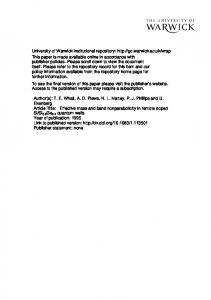
The defects in a crystal can be classified in a number of different ways. One of the first important distinctions to make is between point defects and extended defects. Throughout this thesis a point defect will refer to a defect which can be considered as a “molecule trapped into the lattice structure”. The size of these ’molecular’ defects rarely exceeds that of the unit cell shown in Figure 1.1. An extended defect refers to structures which span multiple unit cells; these can include voids, dislocations, inclusions or grain boundaries. This thesis is concerned with the study of point defects. Extended defects will only be referred to with regard to the influences these may have on the aggregation kinetics of the systems. In 1934 Robertson et. al. realised that diamonds could be separated into two classifications by examination of their IR absorption spectra [11]. The most abundant of these were characterised by a particular set of absorption lines which were not present in the second type of diamond. It was proposed, then, to divide diamonds into two groups: Type I, where this set of absorption lines were present; and type II where these features were absent. It has since been discovered that the difference between the diamond types was due to the presence of nitrogen, or the lack thereof. The categories proposed by Robertson et. al. are still used today, however, further subdivisions have been added to the system. Figure 1.2 shows the breakdown of these categories.


5

Type Ia diamonds are those for which the defect content is comprised primarily of nitrogen in an aggregated form. In this case the nitrogen can be predominantly in the form of A-centres (two adjacent substitutional nitrogen atoms) [12] or a Bcentre (four substitutional nitrogen atoms surrounding a vacancy) [13]. These two types further subdivides type Ia diamonds into type IaA or IaB samples. Those which have comparable concentrations of A and B centres are referred to as type IaAB diamonds. Samples in which single unaggregated nitrogen centres (NS ) are in abundance compared to other defects are known as type Ib diamonds. Type II diamonds are those which do not have detectable concentrations of nitrogen (< 1 – 2 ppm of any of the forms mentioned above) by IR absorption spectroscopy [14]. If neutral single substitutional boron can be detected by IR in the sample then it is classified as type IIb [15] [16] whereas if neither this nor nitrogen can be detected then the sample is referred to as type IIa. The addition of boron into the diamond lattice introduces a state into the band gap at 0.37 eV above the valance band [17]. The introduction of this acceptor changes the conductivity of the diamond such that it can behave as a semi-conductor, metallic conductor or superconductor by careful control of the boron concentration [18].

1.4

Synthetic diamond

The first reported synthesis of diamond was made in 1955 by Bundy et. al. [19]. The method used for this production is now referred to as high pressure high temperature (HPHT) synthesis. The growth of single crystal synthetic diamonds in this manner is carried out by dissolving graphitic carbon in a molten catalyst (which is generally a transition metal such as nickel or cobalt) and allowing it to diffuse to the growth surface by applying a temperature gradient. High pressures are required to bring the carbon into the diamond stable region of its phase diagram. Since the initial report of synthetic diamond growth by the HPHT method it has been brought to light that the ’synthetic’ diamond produced by Bundy et.


6

al. was actually a fragment of a diamond seed used to attempt the growth [20]. Nevertheless, the technique used was sound and has paved the way for significant developments in the field of HPHT diamond growth. Diamond can also be grown at low pressures by chemical vapour deposition (CVD). The earliest claim of low pressure synthesis was made by Eversole in a patent filed in 1958 and granted in 1962 [21]. CVD growth relies upon the chemical kinetic processes in the growth environment as opposed to the thermodynamically favourable conditions which are relied upon for HPHT growth. A growth mixture of at least hydrogen and carbon, a seed and a method for heating the gas is required for CVD growth. The quality and defect incorporation of CVD synthetic diamond can be carefully controlled by the regulation of the growth temperature and other gasses which are allowed into the growth chamber. It is possible to grow exceedingly high quality (low defect content) diamond using this technique and also to tailor the properties of the diamonds to specific technological applications. This makes CVD diamond a powerful material for the future of many industries.

1.5

Applications of diamond

Not only are the extreme properties of diamond themselves very impressive and unusual but the combination of these properties in a single material makes diamond uniquely suited to a range of applications. A few shall be listed here: • Abrasives: It was mentioned earlier that diamond was used even in early days for scratching other hard materials. In modern times this has not changed. Diamond and diamond composites are used extensively as coatings for drill bits, saws and other mechanical devices which undergo severe abrasion [22]. • Thermal management: In most materials a high thermal conductivity is directly related to a high electrical conductivity because the heat is carried through the material by electrons. In diamond it is the phonons which mediate the heat through the crystal and this is significantly more efficient.


7

For this reason diamond can be used as a heat spreader for a wide range of applications, in particular high power electronics [23]. • Optical windows: The broad optical transparency of diamond makes it a very useful material for optical components such as optical windows [24]. The use of diamond as an active optical element in Raman lasers is also a growing and technologically important field of research [25]. • Water treatment: Boron doped diamond is now being used as an electrode material for the electrochemical treatment of water which contains organic pollutants [26][27][28]. The wide potential window in aqueous solutions and the chemical stability make it an ideal material for this application. • Medical devices: Because diamond is biologically inert it can be used in a range of medical devices. Polycrystalline diamond has been used to make artificial joints which have long wear resistance. Single crystal diamond scalpels are also highly valued by ophthalmologists for use in eye surgery [29]. • Speaker systems: Diamond is a light weight and stiff material making it ideal for the production of high frequency tweeters in speaker systems for top of the range audio devices [30]. • Radiation detectors: The radiation hardness of diamond means that prolonged use does not lead to leakage currents until very large doses of radiation have been received. CVD Diamond is now regularly used in radiation detector apparatus due to its large electron/hole mobility and its high breakdown field [31][32]. • Both nanoscale magnetometry and nanoscale nuclear magnetic resonance (NMR) have been made possible by the unique properties of the nitrogenvacancy defect in CVD diamond [33][34][35]. The book Comprehensive Hard Materials Volumes 1 – 3 provides a more detailed review of the applications of diamond for abrasives, particle & photon detectors, single colour centre and electrochemical applications [36].


1.6

8

Motivation for study

As mentioned in §1.1 De Beers’ marketing has lead to a significant demand for natural gem stones as opposed to synthetics. Bain & Company provide evidence for this demand from the global population [3]. In 1999 it was reported that HPHT annealing had been used to ‘improve’ the colour of brown natural diamonds by General Electric (GE) (the patent having been submitted in 1997) [37]. Such treatments could turn a brown diamond a number of different colours depending on the constituents of the as-mined sample but most frequently would simply make the sample colourless or near-colourless. At first it was thought that these samples were indistinguishable from untreated samples, however, it was later shown by Fisher that careful analysis could indeed distinguish between these [38]. The annealing of brown CVD diamond also results in the improvement of the sample colour [39]. It is now possible to purchase colourless synthetic diamond gem stones which are in excess of 1 carat (200 mg). The further study of the effects of treatments, such as annealing and/or electron irradiation, on CVD diamond have resulted in a broad spectrum of colours now being available. For example, pink colours are commonly produced by the HPHT annealing, electron irradiation and further annealing to temperatures in the vicinity of 800 – 1000 ◦ C [40]. The treatment of diamond to produce attractive colours has become such a valuable area of research to the extent that many patents have been filed in order to protect the production of specific colours. A review of the patents on this subject up until 2009 is provided by Schmetzer [41]. In order to protect consumer confidence in the $72 billion market for natural diamond jewellery it is imperative to be able to track the growth and treatment history of natural and synthetic diamonds. In addition, the identification of new defects may lead to the discovery of a defect centre with as many useful technological applications as the well known nitrogen-vacancy centre. Finally, if diamond


9

is to be used in extreme environments in which the sample may experience irradiation, heating or both, it is essential that there is a thorough understanding of the effects of these treatments. Without understanding the changes to the defect content it will not be possible to use this extraordinary material to its full potential. In the research presented in this thesis a number of experimental techniques will be employed in order to study the change in the defect content in CVD diamond samples subjected to a range of treatments. EPR is a powerful technique which allows not only the physical and electronic structures of defects to be probed but also allows quantitative measurements of those defect centres. UV-Vis and IR absorption spectroscopies will be used to track defect concentrations (where the defect corresponding to an optical feature is known) and identify optical analogues for new EPR active defects. Photoluminescence is a highly sensitive technique which allows for the identification of defect centres which are not detectable via UV-Vis absorption, adding extra versatility to the study.

1.7

Thesis outline

This thesis contains four background chapters, four experimental chapters and a chapter to summarise the results of the thesis as follows: • Chapter 1 discusses the history of diamond, its structure and properties, and the applications to which it can be applied. The chapter is concluded with the specific motivation for this study. • Chapter 2 provides a tailored review of the field of diamond research, particular emphasis is placed upon the difference in defect content between HPHT and CVD synthetic diamond. • Chapter 3 details an overview to the theory of the techniques used in this thesis. EPR, optical absorption and photo-luminescence are described along with the effects of reorientation dynamics on EPR spectra.


10

• Chapter 4 reviews the experimental apparatus which are used throughout this thesis. • Chapter 5 reports the identification of a new paramagnetic defect in annealed CVD diamond. Multi-frequency EPR is employed in the identification of this defect which is shown to be the neutral di-nitrogen-vacancy-hydrogen defect (N2 VH0 ). • Chapter 6 investigates the properties of the di-nitrogen-vacancy-hydrogen defect. A detailed annealing study of CVD diamond is presented to investigate the production of N2 VH0 . A comparison of the charge transfer behaviour of samples which contain N2 VH0 allow for an optical analogue of this defect to be identified. • Chapter 7 reports upon the incorporation of oxygen in diamond grown in a C:H:O plasma. Further evidence is provided for the assignment of the WAR5 EPR signal to the oxygen-vacancy neutral defect (OV0 ) (first proposed by Cann [42]) along with experimental evidence for the presence of substitutional oxygen in the diamond lattice. A previously unreported EPR active defect is identified in diamond grown in a C:H:O plasma and characterised as the oxygen-vacancy-hydrogen defect Os VH0 . • Chapter 8 concerns the effects of irradiating and annealing CVD diamond. It is found that a feature observed in infra-red optical absorption spectroscopy at 3324 cm-1 (Ns :H–C0 ) is produced by irradiation. • Chapter 9 brings together all of the conclusions presented in this thesis.

Chapter 2 Literature review The purpose of this chapter is not to review the field of diamond research in its entirety, as that is beyond the scope of this thesis. Instead the review aims to provide the reader with the background necessary to appreciate the motivations and implications of the work presented in this thesis. The growth techniques implemented in the production of synthetic diamond shall be outlined and this will be followed by a focussed review of the different defects incorporated in HPHT and CVD diamond samples. Finally, a short review of irradiation damage defects in diamond is presented.

2.1

Growth methods

At standard temperatures and pressures graphite, not diamond, is the thermodynamically stable allotrope of carbon [5]. This means that in order to grow diamond we must either make the thermodynamic or chemical kinetic conditions favourable: the two techniques described in this chapter, HPHT and CVD synthesis, satisfy each of these conditions, respectively. Figure 2.1 shows the carbon pressure-temperature diagram on which the regions for catalytic HPHT synthesis and CVD synthesis have been highlighted.

11

Chapter 2. Literature review

12

30

Pressure (GPa)

Diamond

Liquid

20 HPHT Catalytic Synthesis 10 CVD Synthesis 0

0

1000

2000

Graphite

3000

4000

5000

6000

Temperature (K) Figure 2.1: The phase diagram of carbon bounded to the regions which are of interest for the growth of diamond. Catalytic HPHT and CVD growth have been illustrated. Adapted from [50]. The pressure required for CVD growth has been exaggerated for clarity [23].

This thesis is concerned with the defect aggregation in single crystal diamond and will therefore not discuss the methods for growth of poly-crystalline diamond (PCD) or nano-crystalline diamond (NCD). Discussions of the synthesis of these forms of diamond can be found elsewhere [43] [44] [45] [46] [47] [48] [49].

2.1.1

HPHT diamond synthesis

As mentioned in Chapter 1, the first successful growth of diamond used high pressures and temperatures in conjunction with a metal catalyst in order to bring the experimental conditions into the diamond stable region of the carbon phase diagram [19]. In all High Pressure High Temperature (HPHT) synthesis of large single crystal diamond, seeds are placed in a capsule along with a metal solvent-catalyst and a high purity source of carbon. The seeds are generally either natural or synthetic diamond samples (homoepitaxial growth). The metal solvent takes the form of a 3d transition metal: typically nickel, iron, cobalt or a eutectic of these. This solvent, or ’flux’, acts as a transport agent for moving carbon between the carbon


13

source and the seeds [5]. The metal solvent also acts as a catalyst which lowers the temperature required for direct conversion to diamond [50]. Typical conditions for catalytic HPHT growth are 1200 - 1500 ◦ C at between 5 and 6 GPa [51] [52] [53] but a wider range of temperatures and pressures may be used. There are a number of different press systems which can be used to apply pressure during growth but it is beyond the scope of this thesis to review all of these. The author directs the readers to a number of review articles and papers on the subject: [5] [41]. The temperature is controlled by resistive heating of either the entire capsule or internal components of the capsule [19] [54].

2.1.1.1

Defect incorporation in HPHT diamond

Nitrogen is the major impurity in HPHT grown diamonds. Nitrogen is incorporated into the growth from sources such as: the air; impurities in the metal solvent; adsorbates to the capsule components; the carbon source. Nitrogen typically incorporates in the form of single nitrogen atoms substituting for a carbon at a lattice site, commonly referred to single substitutional nitrogen (Ns ) [55]. Where no measures are taken to reduce the nitrogen content in the growth, single substitutional nitrogen can incorporate at concentrations of hundreds of parts per million (ppm) [56]. Some nitrogen aggregation can occur during growth if the temperature is high enough whereby single substitutional nitrogen atoms migrate to one another forming the more stable A-centre (two nearest-neighbour substitutional nitrogen atoms) [57]. The nitrogen content can be controlled by including a nitrogen-getter in the solvent [58] [59]. These getters have a large affinity for nitrogen and so prevent it from incorporating into the final diamond product. Aluminium and titanium are regularly used as getter elements [60]. The drawback of using such elements is that they can be incorporated into the diamond instead of nitrogen, albeit at significantly lower concentrations and often in the form of inclusions [61]. An alternative to nitrogen getting is to degas the growth capsule, removing all atmospheric gasses [51]. Once the capsule is degassed it is also possible to then purge the capsule with


14

a desired gas in order to intentionally dope the resultant diamond with other impurities. Such intentional dopants might include boron, to change the conductivity of the sample, or isotopically enriched

15

N.

To date, only one defect containing hydrogen has been reported in as-grown HPHT diamond. This defect, incorporating both oxygen and hydrogen, was characterised as the V(OH)0 defect and was produced in a sample grown in a carbonate medium (Na2 CO3 – CO2 – H2 O – C) [62]. This defect will be discussed further in Chapter 7. In annealed HPHT grown diamond it has been found that a feature arising at 3107 cm-1 is produced. This feature has been identified as arising from an aggregate of three substitutional nitrogen atoms and one carbon atom surrounding a vacancy in which a hydrogen is bonded along the carbon-vacancy bond direction [63]. This suggests that hydrogen is incorporated into the diamond during growth in a form which has not been detected by FTIR. Since only these two defects have been identified as containing hydrogen in HPHT grown diamond it is assumed that very little hydrogen incorporates into the diamond lattice compared to the level of nitrogen incorporation.

2.1.2

CVD diamond synthesis

Where HPHT diamond synthesis seeks to satisfy thermodynamic conditions in order to form diamond, CVD growth instead exploits chemical kinetics to produce the desired end product [64]. In order to grow diamond in this manner a source gas containing at least carbon and hydrogen (often in the form of hydrocarbons) is heated such that these compounds break up to form carbon and hydrogen radicals. This process takes place above a seed material which, for single crystal growth, is diamond. The carbon in the gas phase deposits epitaxially onto the growth surface. The hydrogen species in the system preferentially etch carbon which hybridises in an sp2 graphitic form, allowing for the growth of sp3 diamond instead [64]. Hydrogen also serves to stabilise the sp3 carbon growth surface.


15

Figure 2.2: A simplified depiction of the C:H:O phase diagram for CVD growth first reported by Bachmann [71].

A number of methods exist in order to dissociate the reactants in the gas phase. The most simple method is by using a hot filament close to the substrate at 2000 ◦ C. This technique is simple in design; however, samples grown in this manner are vulnerable to incorporating impurities from the filament material itself [65]. A second commonly used method is to heat the reactants in a cavity using microwaves, resulting in a plasma above the growth substrate [66]. This method, referred to as microwave plasma CVD (MPCVD), is the subject of a large portion of the literature of CVD diamond growth [67] [68]. Microwave sources of 2.45 GHz were widely available in the mid-1900s as these sources were first used for radar applications during WWII and later these frequencies also became the standard for microwave ovens [69]. Using this technique removes the possibility of incorporating elements from the heating source. Unless care is taken, other contaminants can be introduced into the gas phase. Silicon, for example, can be etched from reactor windows and incorporated into the lattice [? ]. Studies by Bachmann showed that a range of ratios of the carbon:hydrogen:oxygen content can be used to grow diamond by the CVD method [71]. These results were taken from over 75 CVD growth experiments and are summarised in the C:H:O phase diagram shown in Figure 2.2. Each axis in the figure shows a ratio of atomic incorporation with respect to two elements in the system. If the growth chemistry


16

contains all three elements then it will be located inside the triangle. Any growth chemistries only involving two elements will be accounted for along one of the axes. As shown in the figure, only a very limited range of growth chemistries will allow for the growth of diamond by the CVD method. Further studies have subsequently been performed on the growth of diamond in C:H:O plasmas which have all agreed with the findings of Bachmann [72][73][74][75][76]. Adding oxygen to the growth chemistry serves to assist in etching sp2 carbon from the growth surface resulting in higher quality growth [77]. Oxygen has also been used when growing boron doped CVD diamond to inhibit the growth of undesirable {110} faces when growing in an (001) plane [78]. Conflicting reports have been made about the influence of oxygen on the growth rate of CVD diamond [79][80][77]. The optimisation of diamond growth rates and quality by MPCVD is not a simple goal to achieve. A large number of parameters can be varied to this end: the reactor design; the temperature; the carbon-hydrogen ratio; other source gas additives [81]; microwave frequency [82]; the plasma power density at the sample. In addition to the variables which are used to alter the growth environment it is also possible to vary the substrate seed. The highest quality growth has been achieved on {001} oriented diamond substrates [83]. The type of substrate and its orientation can have significant effects on the potential growth rate and quality of the final material [84]. Tallaire et. al. provide a review of recent achievements and remaining challenges (such as larger crystals, cheaper production and faster growth) in the growth of CVD diamond [83].

2.1.2.1

Defect incorporation in CVD diamond

Extended defects on the surface of a growth substrate have been shown to propagate through newly formed diamond layers resulting in large dislocation densities in the final material. Such extended defects can induce large amounts of strain in the crystal which can affect the birefringence and thereby its use in optical applications. High dislocation densities also reduce the effectiveness of CVD diamond


17

as a detector material [85]. It has been shown that chemical etching of the substrate can help to remove some of the damage from abrasive substrate preparation techniques and so reduce dislocation densities [86]. The nitrogen incorporation efficiency during CVD growth (probability of nitrogen incorporation as compared to carbon) is only 0.001 - 0.01%; however, it is still one of the dominant impurities found in diamond grown this way [87] [88]. It is difficult to exclude all sources of nitrogen from the growth environment and source gasses. This can be a severe problem for technological applications [89]. It has been shown that including even small concentrations of nitrogen in the source gas can significantly increase the growth rate of the CVD diamond [90][91]. Growth rates as high as 150 µm/h have been reported but such samples generally have a brown colouration [92]. Positron annihilation studies have shown that brown CVD diamond contains vacancy clusters [93]. It has also been demonstrated that the origin of the brown colour in CVD diamond is not the same as that for brown colour in natural diamonds [94]. It has been shown that annealing at 1600 ◦ C can remove this brown colour. Nitrogen can incorporate in a number of different forms. The most simple and abundant of these is in the single substitutional form mentioned in §2.1.1.1. In this case a nitrogen atom becomes bonded to the diamond surface during the growth process and is grown over by carbon atoms. Single substitutional nitrogen, in its neutral charge state, is EPR active and has been recognised in natural diamond since 1959 [95]. Ns is also regularly observed in HPHT and CVD synthetic diamonds. The defect can also exist in the negative and positive charge states [96] [97]. The positive charge state is commonly observed in CVD diamond when other defects which act as acceptors are present. The nitrogen-vacancy centre is composed of a substitutional nitrogen atom adjacent to a vacancy. It has been shown by Edmonds et. al. that nitrogen-vacancy centres can grow into the diamond with preferential orientation in (110) grown diamonds. This suggests that the NV centres are formed as a unit during growth


18

and that vacancies are not migrating through the lattice to Ns centres [98]. It has also been shown that it is possible to grow nitrogen-vacancy centres with 94 % preferential orientation along a single crystallographic direction on (111) oriented substrates [99]. The nitrogen-vacancy centre in the negative charge state is one of the most studied defects in solid state systems. In its negative charge state the defect has an S = 1 spin ground state and C3v symmetry [100]. This defect is routinely detected by EPR and also has an optical zero phonon absorption at 637 nm. In the defect’s neutral charge state it is expected to have an S = 1/2 spin ground state but it has never been detected by EPR. This is believed to be due to dynamic JahnTeller distortions which result in the broadening of the defect beyond observation [101]. An excited S = 3/2 state of NV0 defect has been observed under optical illumination in EPR [101]. More details about the annealing behaviour, spin polarisation properties and production mechanisms for this defect are provided in Chapters 7 and 8. Edmonds et. al. showed that the nitrogen-vacancy-hydrogen defect (NVH) could also be grown into CVD diamond samples with preferential orientation [98]. In this defect it has been shown that the hydrogen reorientates between the three equivalent nearest neighbour carbon atoms to the vacancy [4]. The NVH defect centre incorporates into CVD diamond at a greater concentration than the NV centre, presumably because of the large amounts of hydrogen in the source gas [98]. It is unclear, however, whether the hydrogen is grown into the NVH centre or if mobile hydrogen migrates to an NV centre during growth. It has been shown by Stacey et. al. [102] that hydrogen can diffuse through the near surface of CVD diamond at temperatures similar to the CVD growth temperature. Diamonds which have been annealed produce higher aggregates as defects migrate through the crystal lattice. A and B centres were mentioned in Chapter 1, for example. Other aggregates involving multiple nitrogen atoms, vacancies and hydrogen atoms can also be formed. Chapters 5 and 6 will discuss these in more detail.


19

As mentioned earlier, silicon can be incorporated into the diamond lattice. This can either be intentional, by including silicon species in the growth chemistry, or unintentional, by the etching of reactor windows. It is proposed that silicon incorporates primarily in the form of substitutional silicon. While substitutional silicon has not been directly observed, it has been demonstrated that the silicon vacancy defect can be produced by irradiation and annealing, implying the presence of substitutional silicon in the lattice [103] [104]. In silicon vacancy defects, the silicon atom resides halfway between two vacancies [4]. It has been shown that the silicon vacancy can also be grown into the lattice with preferential orientation suggesting that it too is grown into the lattice as a unit [105]. A hydrogen analogue of this defect has also been identified in CVD diamond and has been shown to preferentially orientate when grown on a (110) substrate [? ]. The neutral silicon-divacancy-hydrogen defect centre has also been identified by EPR [? ]. Hydrogen is the most abundant element in the gas phase during the CVD diamond growth and it is therefore potentially one of the primary impurities in single crystal (SC) CVD diamond. It is unclear exactly how much hydrogen is incorporated into SC CVD diamond. Some natural and polycrystalline diamonds have shown hydrogen concentrations as high as 1 atomic percent [106]. Dischler et. al. showed that some of this hydrogen may be trapped in dislocations or at grain boundaries [106]. EPR studies have shown that hydrogen is incorporated into the bulk of the diamond lattice [107] [108] [109] [110]. Further IR features have been shown to arise from C – H stretch and bend modes by isotopic substitution of hydrogen for deuterium [111] [42] [112]. Theoretical calculations suggest that interstitial hydrogen is stable at the bond centred site but that such defects would not be IR active [113]. A di-hydrogen structure is believed to have a lower energy than the single interstitial hydrogen [114]. Hydrogen interstitials are discussed further in Chapter 8. Despite the use of oxygen in CVD diamond growth, only one point defect to date has been identified to involve oxygen in such material. The EPR active signal


20

WAR5 has been proposed by Cann to arise from the neutral oxygen-vacancy defect - an electronic and structural analogue of the nitrogen-vacancy defect [42]. It was suggested by Cann that some further work was required before it was proven conclusively that this defect is indeed the oxygen-vacancy. Cann’s evidence will be provided in Chapter 7 along with a more in depth discussion of oxygen related defects in diamond.

2.2

Irradiation of diamond

Irradiation of diamond was first commented upon by Sir William Crookes in 1909 in his book simply entitled ‘Diamonds’ [115]. In this book Crookes noted how exposing a diamond to a radioactive radium source for 12 months resulted in the samples turning a ‘bluish-green colour’. It was noted at this time how the colour change increased the value of the diamonds because of the ‘fancy’ colours which were produced. Unbeknownst to Crookes, the radiation produced by his radium sources resulted in the production of vacancy and interstitial defects in the diamond. The irradiation of diamond results in the displacement of host atoms if the incident radiation imparts energy greater than the displacement energy to the atoms. The sites which are vacated are referred to as vacancies and can be detected optically by absorption and photo-luminescence measurements or by EPR. The displaced atoms which no longer reside on a lattice site are called interstitials. Some forms of interstitials have been observed in optical absorption and EPR but it is unknown if interstitials can also exist in configurations other than those reported in the literature. The defects which are produced by irradiation are highly dependent on the defect content in the diamond. In this section, two broad categories will be considered: type IIa diamonds, in which the Ns content is negligible; and type Ib diamonds, in which the Ns concentration is significantly greater than the radiation damage defect concentrations in the diamonds.


2.2.1

21

Irradiation damage in type IIa diamond

In the neutral charge state the zero phonon line of the vacancy is observed as a doublet at 741.1 nm and 744.6 nm. The two zero phonon lines and their associated vibronic band are collectively referred to as GR1 (standing for General Radiation 1) [116]. The absorption features GR2-8 also arise from electronic transitions of the neutral vacancy [117] [118]. Theoretical analysis, first performed by Coulson & Kearsley, of the neutral vacancy has assigned the doublet transitions between a 1 E ground state and a 1 T2 excited state with Td symmetry [119] [120] [121] [122] [123] [117] [124] [125]. Uniaxial stress measurements have confirmed these theoretical predictions [126] [127]. In EPR the neutral vacancy is normally undetectable due to an S = 0 [128] ground state, but under optical illumination of energy in excess of 3.1 eV the defect can be observed in an S = 2, 5 A2 excited state [129]. Annealing irradiated type IIa diamond to temperatures at which the vacancy is mobile (> 900 K) results in the formation of the neutral di-vacancy, two nearest neighbour vacancies. Prolonged annealing at temperatures above 1100 K results in the annealing out of this defect. The defect is shown to have C2h symmetry at low temperatures (∼ 80 K) and has been correlated with the TH5 optical absorption band [130]. Many different possible sites for interstitials exist but it has been predicted that the 〈001〉-split interstitial is the lowest energy configuration [131][132][133]. This defect has D2d symmetry and an S = 1 excited state which has been associated with the R2 EPR centre [134]. Optical transitions at 735.8 nm and 666.9 nm have also been attributed to the 〈001〉-split interstitial [135][136][137]. No other charge states of the interstitial have yet been identified but charge transfer experiments suggest that at least one other charge state does exist [138]. The di-〈001〉-split interstitial complex has been observed by EPR in irradiated IIa diamond [139]. This suggests that the interstitial, or at least a fraction of the interstitials, are mobile under irradiation conditions, even when the treatment


22

is performed at temperatures below 100 K [140]. The activation energy for the annealing of the interstitial has been measured as 1.68(15) eV [141] but low temperature irradiation would not provide this degree of energy. This has lead to the hypothesis that a highly mobile form of the interstitial, I* , is present under irradiation. It has been proposed that I* has a migration energy of ∼ 0.3 eV [142]. The tri-[001]-split interstitial, O3, is produced in IIa diamond which has been irradiated at 100 K. The centre is removed after annealing at 680 K [143]. The S = 1 ground state of this defect has been identified by EPR and has been shown to have a C2 ground state with a 〈001〉 rotation axis. DFT calculations were used to provide further evidence that the assignment of the tri-[001]-split interstitial model to the O3 EPR centre was correct [144]. With an activation energy of 1.68(15) eV, a reduction in the neutral vacancy concentration is observed [141] alongside a narrowing of the ZPL by a factor of two after annealing at around 450 ◦ C [145]. This loss of vacancies has been attributed to the recombination of nearby vacancies and interstitials. Nearby vacancies and interstitials cause increased strain in the lattice, leading to a broad ZPL. The resulting reduction in strain in the lattice from the recombination of these has been proposed as the reason for the narrowing of the ZPL [142][141]. Further annealing of the vacancy is attributed to its migration and capture at other impurity sites or surfaces [146]. This process occurs with an activation energy of 2.3(3) eV [147][142].

2.2.2

Irradiation of type Ib diamonds

When there is a large concentration of Ns in the diamond with respect to the irradiation damage, the charge states of the defects produced will differ to those observed in type IIa diamond. Nitrogen can also capture interstitial defects forming defects which are not present in type IIa diamond and thereby significantly altering the aggregation processes in the diamond.


23

The vacancy was first observed by optical absorption in the negative charge state by Dyer et. al. in 1965 [148] but not assigned to arising from V- until 1970 by Davies [149]. The optical feature is labelled as the ND1 centre and has a zerophonon-line at 394 nm. Davies used uniaxial stress measurements to show that the 394 nm ZPL arises from an 4 A2 to 4 T1 transition at a defect with Td symmetry [150]. The negative charge state of the vacancy is EPR active with an S = 3/2 ground state [151]. The concentration of negative vacancies was correlated with the intensity of the ND1 feature in optical absorption by Twitchen et. al. thereby allowing quantitative measurements of the vacancy from optical measurements alone [152]. During irradiation of type Ib diamond, the I0h001i interstitial is still produced at the same concentrations as in type IIa diamond; however, the production of di〈001〉-split interstitials is inhibited [153]. Irradiation of type Ib diamond followed by annealing to 1100 K results in the production of NI [154]. It has been suggested that this defect is in fact formed upon irradiation but it cannot be observed until the signal resulting from the negative vacancy is annealed out at 1100 K. The NI defect has been identified by EPR and shown to have C2v symmetry and an S = 1/2 ground state in the neutral charge state. The defect is expected to be diamagnetic in the negative charge state. Further, the 〈001〉-split nitrogen interstitial-self-interstitial pair (NI -I0h001i ) is formed under the same conditions as the NI defect. The NI -I0h001i defect was also identified by EPR and shown to have C1h symmetry and an S = 1/2 ground state. This defect is analogous to the di-〈001〉-split interstitial with one of the interstitial carbon atoms replaced with a nitrogen instead [154]. Both NI and NI -I0h001i have been shown to be stable up to 1800 ◦ C; this annealing behaviour matches that predicted by theory [155]. The H1a absorption feature in diamond has been assigned to the 〈001〉-di-nitrogensplit-interstitial (N2I ) [156]. This defect is produced in irradiated type Ib diamond after annealing to temperatures above 600 ◦ C. The H1a feature continues to increase in intensity up until annealing at 1200 ◦ C and has been shown to anneal out at temperatures greater than 1550 ◦ C [112].


2.3

24

Other literature reviews through this thesis

At the introduction of each experimental chapter a review will be given of the field pertaining specifically to the work presented therein. These shall be outlined here for reference:

• Chapter 5 discusses the family of Nn V and Nn VH, where n = 1 − 4, with regard to the structure of these defects and the history of their detection by EPR or optical methods (or, in some cases the lack of detection). Finally, the structures of the NVH and N3 VH defects are examined in further detail with particular attention paid to the reorientation of the hydrogen in the NVH defect. • Chapter 6 reviews the aggregation of nitrogen in natural and HPHT synthetic diamonds. Particular attention is paid to the formation of A-centres in diamonds of varying starting Ns concentrations. The annealing behaviour of common defects observed in CVD diamond is then discussed. • Chapter 7 starts by presenting the challenges which are inherent in the study of oxygen in diamond. The evidence provided by Cann for the assignment of the WAR5 signal to the neutral oxygen-vacancy defect is discussed. The neutral oxygen-vacancy is compared to the negative nitrogen-vacancy centre and in particular the spin polarisation and production mechanisms of these defects are considered. Finally, the properties of what might be expected from an Os VH0 defect are presented and compared to the V(OH)0 defect reported by Komarovskikh et. al. [62]. • Chapter 8 reviews the Ns :H–C0 and Vn H- defect structures and the evidence which led to their structural assignements. Theoretical calculations describing the nature of the hydrogen interstitial are also discussed.

Chapter 3 Theory It is the purpose of this chapter to discuss the theory behind the use of electron paramagnetic resonance (EPR), Fourier transform infra red absorption (FTIR), UV-Vis absorption and photo-luminescence (PL) spectroscopies in order to study point defects in semiconductors and insulators. Establishing the symmetry of a defect is vital to the process of determining its structure. To this end a short section on symmetry theory will be presented. The cage model, first used to model diamond by Coulson and Kearsley is presented and used to describe the vacancy. Finally the effect of dynamic reorientation of defects on EPR spectra is discussed.

3.1

Electron paramagnetic resonance

EPR is a powerful technique for the characterisation of paramagnetic point defects in diamond. It can be used to gather information about the symmetry, constituent nuclei and structure of defects. It is not within the scope of this thesis to provide a comprehensive treatment of EPR and so instead an abridged account of the theory will be provided. Many more extensive treatises on the theory of EPR can be found elsewhere [157][158][159][160].

25

Chapter 3. Theory

3.1.1

26

Electron magnetic dipole moment

The manipulation of electron magnetic moments is the basis for EPR. In the simple case one can consider the orbit of a charged particle of charge q moving with a velocity v. For an electron of mass me this gives rise to a current of I = qv/2πr. A magnetic moment, µd is produced equal to the area enclosed by the charge multiplied by the current. Applying a classical treatment we find that: |µd | = IA =

qv 2 q q πr = me vr = l 2πr 2me 2me

(3.1)

where l is the classical orbital angular momentum. Now that the classical case has been analysed it is possible to replace the classical angular momentum with the analogous quantum mechanical operator, ˆl. The eigenvalues resultant from this system are: |µd | =

q ˆ l = |γe ~ml | 2me

where ml = −l, −l + 1... l

(3.2) (3.3)

where γe is the gyromagnetic ratio and ml represents the possible quantised states in which the orbital angular momentum, l, can exist for the system. The total angular momentum of a system is denoted by the operator ˆ j which is comprised of the sum of the orbital angular momentum operator, ˆ l, and the spin angular momentum, sˆ. An electron in an s orbital would have an orbital contribution to its magnetic moment of l = 0 and so the magnetic dipole moment of the system can be defined entirely by the expression: µ ˆS = −

e~ ge sˆ = −ge µB sˆ 2me c

(3.4)

where µB is the Bohr magneton and ge is the free electron g-factor which is equal to 2.002319304386(20)[157]. For a system with no contribution from the orbital angular momentum the energy of a magnetic moment in the presence of a magnetic

Chapter 3. Theory

27

field is given by: H = −µ.B ˆ = ge µB sˆ.B.

(3.5)

From this equation, the energy of the system is dependent upon the eigenstate of the spin. By applying the magnetic field, the degeneracy of the states is lifted and it is the transitions induced between these energy levels which are detected in an EPR experiment. For the case of multiple electron spins in a system, an effective spin can be defined ˆ = sˆ1 + sˆ2 . The effective spin is not a true spin but a whereby, for two spins, S useful model. If sˆn is written as α(n) in the spin up state and as β(n) in the spin down state (in this case where n = 1 or 2), then the possible combinations of spin states can be written as either symmetric or anti-symmetric with respect to the exchange of the electrons [157]: Symmetric α(1)α(2) 1 √ [α(1)β(2) + β(1)α(2)] 2 β(1)β(2) ˆ=1 Triplet state, S

Anti-symmetric 1 √ [α(1)β(2) − β(1)α(2)] 2 ˆ=0 Singlet state, S

ˆ + 1) of the symmetric state is equal to three this state Since the multiplicity (2S ˆ = 0 case is referred to as a singlet is called a triplet, while the anti-symmetric S state.

3.1.2

Resonance conditions

An electron has two possible values of its spin state: ms = +1/2 or −1/2. From Equation 3.5 the presence of a magnetic field acting on an electron results in an energy separation of ∆E = ge µB B between the two possible energy states of the electron. The energy required to drive a transition between these two states can be provided by the magnetic field component of an electromagnetic wave, Bmuw ,

Chapter 3. Theory

28

with frequency νµw under the condition that: ∆E = hν = ge µB B

(3.6)

where B1 B and B1 ⊥ B. This means that EPR can theoretically be performed at any frequency so long as the corresponding static magnetic field is achievable for the system. Commonly used frequencies are 9.8 GHz and 34 GHz which correspond to B field values of 0.35 T and 1.2 T, respectively for ge . This is primarily due to the microwave sources which were readily available when EPR was first developed [69]. From Equation 3.6 it is clear there are two possible ways to perform an EPR experiment: By maintaining a static frequency and sweeping the magnetic field or by applying a set magnetic field while changing the applied frequency. In this thesis only the former case, commonly referred to as continuous wave (CW) EPR, will be dealt with. Details of how the EPR experiments have been performed are dealt with in Chapter 4.

3.1.3

The spin Hamiltonian

The most simple system has now been considered: one which consists of only a ˆ single electron. The addition of further electron spins requires the effective spin, S to be considered. The effect of other electron and nuclear spins and the interactions resulting from these is described by the effective spin Hamiltonian [157]: ˆ ˆ ˆ+ H = µB S.g.B + S.D. S | {z } | {z } 1

2

X j

ˆ [S.A .Iˆj − µN gN Iˆj B + Iˆj .P .Iˆj ] | {zj } | {zj } | {zj } 3

4

(3.7)

5

where Iˆ j is the effective nuclear spin operator for the jth nucleus. Higher order terms also exist in the Hamiltonian but these will not be considered in this simple treatment. The terms labelled 1-5 represent the following:

1 Electronic Zeeman interaction

Chapter 3. Theory

29

2 Zero-field interaction (where S > 1) 3 Hyperfine interaction 4 Nuclear Zeeman interaction 5 Nuclear quadrupole interaction (where I > 1)

3.1.3.1

Electronic Zeeman interaction

As discussed in §3.1.1, the electronic Zeeman interaction arises from the interaction between the electron dipole moment and the magnetic field. When the orbital angular momentum is non-zero, this can be written as:

ˆ + gS ˆT ) HZe = µB B.(L

(3.8)

The coupling between the spin and orbital angular momenta must be considered. These can be represented as an additional term in the spin Hamiltonian equation: ˆ X SˆX + L ˆ Y SˆY + L ˆ Z SˆZ ] ˆ T .S ˆ = λSO [L HSO = λSO L

(3.9)

which, upon combining with the Zeeman interaction from both the electron spin and the orbital angular momentum, leads to: ˆ + ge S) ˆ + λSO L. ˆS ˆ H = HZe + HSO = µB B.(L

(3.10)

where λSO is the Russel-Saunders spin-orbit coupling term which describes the strength of the spin-orbit coupling. Using perturbation theory it is possible to determine the effect of the spin orbit coupling on the system. Let the ground state of the system be represented by the wavefunctions |ψ0 , MS i where ψ0 represents the spatial component of the wavefunction and MS represents the spin state. To

Chapter 3. Theory

30

first order we see that: ˆ z |ψ0 , MS i E0 = hψ0 , MS |ge µB Bz Sˆz |ψ0 , MS i + hψ0 , MS |(µB Bz + λSˆz )L

(3.11)

where we have defined the magnetic field (B) to be along the z -axis. The first term in this equation gives the Zeeman energy without any contributions from the orbital angular momentum. The second term can be rewritten as: ˆ z ψ0 i hMS |µB Bz + λSˆz |MS ihψ0 |L

(3.12)

The expectation value of the orbital angular momentum operator for two wave functions, n and m, is be given by[161]: ∗ ˆ ˆ hn|L|mi = −exp[i(ϕn − ϕm )]hn|L|mi

(3.13)

For wavefunction n, ϕ is defined by: n = |exp(iϕ)|2 n. With this knowledge it is evident that where m = n: ˆ ˆ ∗ hn|L|ni = −hn|L|ni

(3.14)

Equation 3.14 can only remain valid if the expectation value is imaginary. Since ˆ is an observable it must be real and thus can only be equal to zero. Applying L this to Equation 3.12 it is evident that to first order the spin orbit coupling does not affect the energy of the system and so second order perturbation theory can be applied. X |hψ0 , MS |(µB B + λS) ˆ T .L ˆ + ge µB B T .S|ψ ˆ n , MS0 i|2 H =− En − E0 ψ 6=ψ 0

(3.15)

n

In this case ψn and MS0 result from higher order excited states which mix with ˆ vanishes since hG|ni is zero. the ground state. From this the term in ge µB B T .S

Chapter 3. Theory

31

Expanding the first term on the right hand side of this equation yields: ˆ + λ2 S ˆT .Λ.S|M ˆ S0 i H = hMS0 |µ2B B T .Λ.B + 2λµB B T .Λ.S

(3.16)

where the following simplification has been made: Λ=−

X hψ0 |L|ψ ˆ n ihψn |L|ψ ˆ 0i En − E0 ψ 6=ψ 0

(3.17)

n

In Equation 3.16 the first term only applies a constant contribution to the energy of each spin state and so does not affect the splitting of the energy levels in any way; it will therefore be ignored [157]. Adding the second and third terms to the result of the first order perturbation then leads to: ˆT .(ge 13 + 2λΛ).B + λ2 S ˆT .Λ.S ˆ H = µB S ˆ+S ˆT .D.S ˆ = µB B T .g.S

(3.18) (3.19)

where 13 is the 3 × 3 unit matrix. It is clear now that any anisotropy which arises in g is due to the spin-orbit coupling matrix, Λ. The second term here is the zero-field interaction which is term 2 in Equation 3.7 and will be discussed next.

3.1.3.2

Zero-field interaction

In a system where B = 0 the (2S + 1) - fold degeneracy of the electronic states can be lifted by the zero-field interaction if the effective spin of the system satisfies S > 1. This interaction is represented by the term: ˆT .D.S ˆ Hzf = S

(3.20)

The zero-field matrix is always made traceless (tr(D) = 0) by subtracting any isotropic component of the matrix. The isotropic component results in a constant

Chapter 3. Theory

32

shift in the energy levels and so makes no difference to the observed EPR spectrum. There are three potential contributors to the zero-field term: • The spin-orbit interaction; This was derived in §3.1.3.1. • The exchange interaction; This describes the direct overlap of the unpaired electrons’ wave functions with one another. Full details of this interaction can be found elsewhere [162]. • Dipole-dipole interactions; This is considered in more detail below. ˆ = sˆ1 + sˆ2 , are The dipolar interaction between two spins, sˆ1 and sˆ2 where S separated by a vector r can be described by: Hdip =

µ0 s1 .r)(ˆ s2 .r) ˆ1 .ˆ s2 3(ˆ 2 s − g1 g2 µB 4π r3 r5

(3.21)

Since the D is traceless only two independent energy parameters are required: 3 D = Dz 2

(3.22)

1 E = (Dx − Dy ) 2

(3.23)

where, following convention, we define Dz to be the principal value and Dy > Dx where Dx 6= Dy . Equation 3.21 can now be rewritten: 1ˆ ˆ Hdip = D{Sˆz2 − S( S + 1)} + E(Sˆx2 + Sˆy2 ) 3 µ0 3 2 2 r2 − 3z 2 where, D = g µB 4π 4 r5 µ0 3 2 2 y 2 − x2 and E = g µB 4π 4 r5

(3.24)

(3.25) (3.26)

It has been assumed that g1 = g2 = g. Here E represents a measure of the rhombicity of the system. For a system which has trigonal or higher symmetry E will be equal to zero. For a defect with Td symmetry D will also be zero.

Chapter 3. Theory

33

Information about the dimensions of a defect can be determined in the case that the dipole-dipole term dominates D. This shows that simply knowing the form of the D tensor allows the extraction of useful information about the structure of a system.

3.1.3.3

Hyperfine interaction

The hyperfine interaction is the results of the magnetic moment produced by a non-zero nuclear spin interacting with the effective electronic spin. This interaction occurs for every j th non-zero nuclear spin and so it is necessary to take the sum over each of these. The hyperfine interaction is therefore written as: H=

X

ˆT .Aj .Iˆj S

(3.27)

j

The wealth of detail made available by this interaction is one of the key aspects of EPR which makes it such a powerful technique for determining defect structure. The hyperfine interaction is composed of an isotropic and an anisotropic component; the Fermi contact interaction and the dipolar interaction, respectively. The former term is generated by the unpaired electron density at the nucleus arising from electrons in the s-orbitals. It is given by: A0 =

2µ0 (gµB )(gN µN )|ψ(0)|2 3

(3.28)

where µN = e~/2mp c and mp is the mass of a proton. gN is the g-factor of the nucleus and |ψ(0)|2 describes the probability density of the electron’s wavefunction at the nucleus. The probability of an electron in a p state being localised at the nucleus is zero and hence does not contribute to the isotropic hyperfine interaction. The dipolar hyperfine interaction results in a change of the magnetic field experienced by the electron from its interaction with the nuclear magnetic dipole moment. The treatment of this is analogous to that for the dipolar interaction as

Chapter 3. Theory

34

presented in Equation 3.21 and can be written as such: Hhf dip =

ˆ ˆ ˆ ˆ µ0 3(S.r)( I.r) 2 S.I ggN µB − 4π r3 r5

(3.29)

By expanding the vectors in this equation and then simplifying the resultant expression the dipolar term of the hyperfine interaction becomes: µ0 ge µB gN µN × 4π     2 r − 3x2 3xy 3xz Iˆ − 5 − 5 5    x r r r    2     2 r − 3y 3yz    ˆ  ˆ ˆ ˆ [Sx , Sy , Sz ] •  − 5  • Iy      r5 r  2    2     r − 3z Iˆz r5

Hhf dip = −

(3.30)

ˆT .T.Iˆ =S

The angular brackets in this equation represent the average over the spatial distribution of the electron wavefunction. Thus, including the isotropic contact term discussed earlier, the full hyperfine interaction can now be expressed by: A = A 0 13 + T

(3.31)

where A0 is tr(A)/3 and 13 is once again the unit matrix. In an analogous manner to that performed to obtain equations 3.22 and 3.23 it is now possible to obtain expressions involving A1 , A2 and A3 which provide information about the system: a = (A1 + A2 + A3 )/3

(3.32)

b = [A1 − (A2 + A3 )/2]/3

(3.33)

c = (|A2 | − |A3 |)/2

(3.34)

Chapter 3. Theory

35

a describes the isotropic component of A. b is the dipolar component of the hyperfine tensor. c gives the rhombicity of the tensor analogously to Equation 3.23. As described by Morton and Preston [163], a comparison of a to b can provide an estimate of the electron localisation at the nucleus in question. An outline of this approach will be presented below: A linear combination of atomic orbitals (LCAO) centred on the atoms constituting the defect can be used to represent the wavefunction of the unpaired electron, Φ. With diamond’s strong and highly directional bonds, this makes for a good approximation. Considering only 2s and 2p orbitals, as will be the case throughout this thesis, the wavefunction may be expressed as: Φ=

X i

η i ψi =

X

ηi [αi (ψ2s )i + βi (ψ2p )i ]

(3.35)

i

where the sum is taken over all i nuclei. Normalisation requires: αi2 + βi2 = 1 and

X

ηi2 = 1

(3.36)

i

α, β and η can then be related to the hyperfine parameters by: a = a∗ αi2 ηi2 and b = b∗ βi2 ηi2

(3.37)

a∗ and b∗ are the values for a and b in which 100% of the electron wavefunction is located in the 2s and 2p orbital, respectively. The values of these constants for atoms pertinent to this study have been tabulated in Table 3.1. It is possible to determine αi2 and βi2 using values for a and b which can be determined experimentally. ηi2 in each case then gives the localisation of the electron at the nucleus under consideration. The hybridisation ratio is defined as λh = (β/α)2 which, for an undistorted sp3 orbital in diamond is equal to 3. This model is simple and has not considered any through-space dipolar coupling or spin polarisation, however, it remains a useful starting point for the interpretation of EPR hyperfine data.

Chapter 3. Theory

36

Nucleus

Natural Abundance (%)

I

1

99.9885(70) 1.07(8) 99.636(20) 0.364(20) 0.038(1)

1/2 5.5857 1,420 1/2 1.4048 3,100 1 0.40376 1,540 1/2 -0.5664 -2,160 5/2 -0.75752 -144

H C 14 N 15 N 17 O 13

gN

a0 /MHz b0 /MHz 90.8 47.8 -67.1 -4,628

Table 3.1: Natural abundances and gN values are quoted from The CRC Handbook [164], whilst isotropic and anisotropic hyperfine parameters for 100% localisation are taken from the paper by Morton and Preston [163]. a0 for 1 H arises from the interaction of an electron in a 1s state while the rest of the a0 hyperfine parameters arise from 2s states and the b0 parameters from 2p states.

3.1.3.4

Nuclear Zeeman interaction

The nuclear Zeeman interaction is directly analogous to the electronic Zeeman interaction. In this case a nuclear spin with I > 0 is considered with a g-factor of gN as opposed to ge and a nuclear magnetic moment equal to µN . This system gives rise to an interaction of the form: ˆ HnZe = −µN gN I.B

(3.38)

The nuclear Zeeman interaction is significantly smaller than its electronic counterpart. The ratio between the mass of a proton and that of an electron, mp /me ≈ 2000, is the reason for the significant difference between these two interactions.

3.1.3.5

Quadrupole interaction

The direction of the nuclear spin angular momentum is directly linked to the axis of symmetry for the time averaged electrical charge distribution of the nucleus, i.e. its shape. For a nucleus with I > 1, an electric-field gradient acting on the nucleus will cause a reorientation of its charge ellipsoid and thereby the direction of its spin. The change in energy as a result of this reorientation gives rise to the quadrupole interaction: T Hqp = Iˆ .P .Iˆ

(3.39)

Chapter 3. Theory

37

As with the zero field interaction in §3.1.3.2, it is common practice to make P traceless by subtracting off any isotropic component to the tensor. Using Cartesian co-ordinates the interaction is commonly written as: Hqp

1 ηq P 2 2 = Pk Iz − I(I + 1) + (Ix − Iy2 ) 3 3

(3.40)

3 e2 qef g Q Pk = Pz = 2 4I(2I + 1)

(3.41)

where

and ηq = (Px − Py )/Pz

(3.42)

In this case −|e|qef g represents the largest magnitude of the electric field gradient seen by the nucleus and |e|Q describes the electrical shape of the nucleus and is set for each isotopic species. ηq is another parameter which describes the rhombicity of this system, i.e. its deviation from axial symmetry about the z-axis.

3.1.4

Transition probabilities

As discussed in §3.1.2, during an EPR experiment transitions between energy level states are driven by the incoming B µw (t) component of an electro-magnetic wave. If we define B µw (t) to be parallel to the x-axis then we can work with the x component of the electron spin Sx . The Hamiltonian for the perturbation caused by this interaction is: Hµw = −µ.B µw (t) = (gµB Sˆx − gN µN Iˆx )Bµw

(3.43)

This can be used to construct the energy matrix for a system with eigenstates denoting the possible spin states for the system where each element of the matrix has the form [157]: hMs0 , m0I |Hµw |Ms , mI i

(3.44)

Chapter 3. Theory

38

The eigenvalues of this matrix give the energy levels of the system. The probability for a given transition, and therefore intensity in an EPR spectrum, is found by taking the modulus squared of Equation 3.44 using eigenstates for the initial and final spin states which define the transition. As shown here, eigenstates for this system are composed of linear combinations of ms and mI states. Interactions of the photon with electron spins require the following selection rules due to the need to conserve momentum: ∆ms = ±1; ∆mI = 0

(3.45)

If, however, contributions from the Hamiltonian terms result in the energy levels becoming similar in energy, the states begin to become mixed and the eigenstates can no longer be described purely as linear combinations of single Ms and mI values but as mixtures of multiple states. This state-mixing leads to transitions for which ∆Ms 6= ±1 and ∆mI 6= 0 have non-zero probability.

3.1.5

Spin relaxation and the Bloch absorption lineshape

Up until this point the discussion of the effective spin Hamiltonian has only considered the energy contributions arising from the magnetic moments of particles and the interactions arising therefrom. This has allowed a detailed discussion of the magnetic field at which a transition is expected to occur for a fixed microwave frequency, ν. No discussion has been made thus far of the form which this resonance might take. In order to do this the relaxation dynamics of the spin in an EPR experiment must be considered. For a system under the influence of an external magnetic field, Bz the bulk magnetisation, M is defined as the sum over the individual magnetic moments, µi which are precessing about the field direction with Larmor frequency ω0 . The net magnetisation along the x and y directions is zero since there is no phase coherence between the spins. For an S = 1/2 system, the population difference between spins aligned parallel, N↑ , and antiparallel, N↓ to the field at temperature T can

Chapter 3. Theory

39

be written as: ∆E N↑ = exp − N↓ kB T

(3.46)

An incoming microwave, the magnetic vector of which is perpendicular to the applied static field, can be described as the sum of its x y and z components: B 1 = B1x + B1y + B1z = B1 cos(ωt)ˆ x + B1 sin(ωt)ˆ y+0

(3.47)

When ω = ω0 the microwave becomes resonant with ∆E and the populations of N↑ and N↓ change. This occurs by a rotation of the magnetic moment from the parallel state through the x and y planes to the antiparallel (higher energy) state. As the net magnetisation is rotated away from z, Mx and My become non-zero. The application of coherent microwaves results in a coherence of the magnetic moments being established. Upon removal of B1 the relaxation of the magnetisation towards Mz is assumed to be exponential with a time constant τ1 . The loss of coherence of the magnetic moments is defined as τ2 . The rate of change of the magnetisation can then be expressed by the Bloch equations: dMx Mx = γe (B0 My − B1 sin(ωt)Mz ) − dt τ2 My dMy = γe (B1 cos(ωt)Mz − B0 Mx ) − dt τ2 dMz Mz − Mz0 = γe (B1 sin(ωt)Mx − B1 cos(ωt)My ) − dt τ1

(3.48) (3.49) (3.50)

where γe = q/2me is the gyromagnetic ratio. With the magnetisation rotating at angular frequency ω the treatment of this system is more easily performed if it is considered in the rotating frame of the magnetisation. To do this the rotating frame will be defined with azimuthal angle, φ: xφ , yφ and z which result in the co-ordinates of the magnetisation being denoted as Mxφ , Myφ and Mz . Taking −γe B0 = ωB the Bloch equations can then be solved for the steady state

Chapter 3. Theory

40

z, B0 (a)

µ

z, B0

µ

ω0

(b)

M µ

µ ω

ω

yφ

yφ y

y φ

φ x

xφ

x

xφ , B1 , M

Figure 3.1: Figure (a) shows a system with an external field, B0 applied along the z axis with magnetic moments aligned along this direction precessing at angular frequency ω0 . Figure (b) shows the effect on M of applying a time varying magnetic field, B1 . The rotating frame is also shown at angle φ from the lab frame. Adapted from Edmmonds [4].

(dM /dt = 0), giving: Mxφ = −Mz0

γe B1 (ωB − ω)τ22 1 + (ωB − ω)2 τ22 + γe2 B12 τ1 τ2

(3.51)

Myφ = +Mz0

γe B1 τ2 1 + (ωB − ω)2 τ22 + γe2 B12 τ1 τ2

(3.52)

Mz = +Mz0

1 + (ωB − ω)2 τ22 1 + (ωB − ω)2 τ22 + γe2 B12 τ1 τ2

(3.53)

Here Mxφ represents the dispersion part of the EPR signal while Myφ represents the absorption component. The latter of these two components is the one normally measured during an EPR experiment. For the steady state approximation to the Bloch equations to be valid the external field, B must be swept slowly compared to the relaxation timescales τ1 and τ2 . Under these conditions the lineshape function Y (B) is given by: Y (B) ∝ Mz0

γe B1 τ2 1 + (B − B0 )2 γe2 τ22 + γe B12 τ1 τ2

(3.54)

Chapter 3. Theory

41

Comparing this to the standard Lorentzian lineshape function: Y = Ymax

Γ2 Γ2 + (x − x0 )2

(3.55)

it is obvious that the expected EPR lineshape should be a Lorentzian with Γ = 1/γe τ2 and amplitude Y (B0 ) ∝ Mz0 B1 provided that γe2 B12 τ1 τ2 1. This latter term is often referred to as the saturation term and as it becomes more dominant (i.e., as B1 increases) the magnetisation of the system tends to zero. This effect is referred to as microwave power saturation and manifests because of an equalisation of the populations between N↑ and N↓ . Other mechanisms may result in a change of the linewidth function and while most of them will not be covered in this thesis, the author refers the reader to Weil and Bolton for a more complete overview [157].

3.2

Optical absorption

3.2.1

Transition probability

In this section I will discuss the way in which electromagnetic radiation (EM), specifically in the IR to UV ranges of the EM spectrum, interacts with a crystal lattice. Absorption requires an electric dipole with which the electric field component of the incoming EM wave can interact. The perturbation caused by the absorption of a photon can be described as a perturbation to the Hamiltonian, ∆Hopt : Hopt = eA0 .re±ik.r

(3.56)

where −er is the electric dipole moment and the incoming photon has been described as a plane wave with amplitude A0 . As for EPR, a matrix can be constructed for which the probability of transition from an initial state, ψi , to final state, ψf , is proportional to the modulus squared

Chapter 3. Theory

42

of the matrix element [165]: W ∝ |hψf |Hopt |ψi i|2

(3.57)

The electric dipole moment selection rules are:

• The dipole moment must undergo a change in parity • ∆l = ±1 in order to conserve momentum • ∆ml = 0, ±1

Once the photon is absorbed the electron in question is excited into a higher energy state. Absorption can only occur if the photon energy is equal to the energy difference between the electron’s current state and an available higher energy state.

3.2.2

Electronic and vibronic transitions

In a solid the discrete available energy levels of neighbouring atoms combine resulting in a continuum of states. This overlap leads to two or more continuous bands in k space. The two bands commonly discussed are referred to as the valence band and the conduction band with the gap between these two taking the name of the band gap. The introduction of impurities into the solid leads to additional states being added into the band gap. With this simple model of the electronic configuration of the energy states for a crystalline solid the possible interstate electronic absorption process can be divided into four categories:

• Intrinsic absorption: Whereby an electron is promoted from the valence band to the conduction band. • Extrinsic absorption: In which an electron is transferred between either the valence or conduction band to a defect state within the band gap

Chapter 3. Theory

43

Conduction Band

E

I

(a)

(b)

Emission Absorption

Absorption

Emission

Absorption

~ω

~ω Zero-phonon transitions

Vibronic transitions

Valence Band Zero phonon line

λ

Q

Figure 3.2: Figure (a) shows both zero-phonon transitions and vibronic transitions between two defect states in the band gap. Q is the configuration coordinate. At zero temperature both absorption and emission processes originate from the ground states but are not required to finish in a ground state. Figure (b) shows how the vibronic bands are observed symmetrically centred about the zero phonon line for an absorption and emission experiment, respectively. Adapted from [165].

• Free carrier absorption: In this case the energy absorbed causes a transition within the continuum of states for a single band • Inter defect state absorption: Whereby an electron is promoted from one defect state in the band gap to another.

The indirect band gap of diamond is approximately 5.45 eV which corresponds to 227 nm light [166]. Extrinsic absorption results in the observation of broad absorption bands since states are available from anywhere within one of the continuous valence or conduction bands to a defect state. The minimum energy for transition of an extrinsic absorption is given by the smallest value of: ∆E = |Ev − Edef ect | or ∆E = |Ec − Edef ect |, where Ev and Ec are the maximum valence band energy and the minimum conduction band energy, respectively. Such broad band absorption has been studied in diamond elsewhere with a comprehensive collection having been collated by Zaitsev [167].

Chapter 3. Theory

44

Of most interest to this thesis are the inter defect state absorption processes. in order to discuss these properly it is necessary to realise that defect states in the band gap do not correspond to only a single energy level but as a set of energy levels as exist for a simple quantum well. The Born-Oppenheimer approximation approximation states that the heavy nature of the atoms in a material simply provide a periodic background potential to the electronic states therefore electronic and nuclear motions may be considered independently. In configuration coordinate diagrams this allows electronic transitions to be represented by vertical arrows and changes in vibrational states to be considered as a change in Q, an overall measure of the total motional atomic energy of the system. This also allows the wavefunction to be written as the product of the electronic, ψ(r), and vibrational, χn (Q) (where Q is the configuration co-ordinate), parts where n is the vibrational quantum number of the electronic state [165]. The shape of the vibrational potential is often considered to be harmonic where V ∝ Q2 . An anharmonic potential would manifest as a distortion to the quadratic approximation but this will not be considered in detail. An example of a configuration coordinate diagram can be seen in Figure 3.2. The zero-phonon absorption energy corresponds to the energy difference between the lowest energy state of the ground state and the lowest energy state of the excited state. A transition for which χf (Q) = χi (Q) is referred to as an electronic transition as there has been no change in Q. Transitions for which χf (Q) 6= χi (Q) are called vibronic transitions. Figure 3.2 shows that for an absorption experiment, the vibronic transitions have a higher energy than the zero-phonon line (ZPL) whereas in luminescence experiments they have lower energy. Vibronic states are not observed as a series of sharp ¯ features but instead, since the thermally excited levels are separated by only hω, they form a vibronic continuum in the observed optical absorption spectrum. The Huang-Rhys factor, S, is a measure of the probability of a transition occurring with no phonon interaction, i.e. a zero phonon transition. At low temperatures an electron is unlikely to have sufficient thermal energy to be excited out of its ground state. This means that the majority of electrons will undergo zero-phonon transitions at low temperatures instead of contributing to the vibronic side band.

Chapter 3. Theory

45

In addition, and more importantly in diamond, the Huang-Rhys factor is temperature dependent. The Huang-Rhys factor is temperature-dependent because of the phonon population factor, and, for many optical centres, this leads to a modest increase (typically a factor of 2 to 3) in the zero-phonon transition probability as the temperature is reduced from 300 K to 100 K or lower. The width of the ZPL also decreases as the temperature is reduced because of the reduction in Lorentzian broadening. Consequently, the ratio of the height of the ZPL to that of the vibronic band is increased by a factor of ≈ 10 to 20 on cooling from 300 K to 80 K. For many optical centres in natural diamonds little improvement is obtained by going to lower temperatures because other factors also lead to a broadening of the ZPLs. However, for some optical centres in diamonds with a very low defect concentration (such as those studied in this thesis) a further substantial narrowing of the ZPL can be obtained by cooling to 4K [168]. Consequently most experiments are performed at cryogenic temperatures, often around 80 K for diamond, in order to facilitate the study of the zero-phonon lines.

3.2.3

Vibrational transitions

§3.2.2 has discussed the consequences of adding states into the band gap along with the electronic and vibronic transitions which can be driven between them. The energies discussed in the chapter typically refer to energies from the NIR to UV ends of the electromagnetic spectrum. Energies lower than this can be absorbed, however, these typically drive transitions between vibrational energy states as opposed to electronic ones. Two different mechanisms exist in covalent solids for coupling to vibrational modes:

• Multi-phonon absorption: A photon interacts with an instantaneous electric dipole produced by two or more phonons • Defect induced one phonon absorption: Where the introduction of a defect into the lattice produces an electric dipole with which a photon can interact

Chapter 3. Theory

46

The lattice symmetry of diamond prevents the production of a spontaneous electric dipole by a single phonon. The interaction of multiple phonons can produce an electric dipole moment with which a photon can interact. Such interactions produce the intrinsic diamond infra red spectrum with absorptions between 165-500 meV (1332-4000 cm-1 ) [24]. The maximum frequency at which a phonon can propagate through a crystal lattice is known as the Raman frequency; for diamond this frequency is 1332 cm-1 [167]. Vibrations at higher frequencies than this cannot propagate through the lattice and are instead localised to the extent of only a few atoms from the defect. Such modes arise at light, strongly bonded defect centres and are referred to as local vibrational modes (LVM). The lifetime of the vibration determines the linewidth of the mode. As temperature decreases, the lifetime of the mode increases thereby leading to sharper spectral lines. It is possible to model the LVM of a defect using a simple model of a set of masses on a spring. The solution for a perfect linear chain is: p ω = 2 k/M sin

qa 2

(3.58)

where a is the nearest neighbour separation and q is the phonon wavenumber, k is the spring constant and M is the mass of the host atom. Consider an impurity of mass m which substitutes for one atom in a chain of heavier host atoms each with mass M . For one of the normal modes of the lattice the vibration will be localised around the impurity atom. In this case the impurity is taken to have the n = 0 position and the lattice equations of motion are: m¨ u = k(u1 + u−1 − 2u0 )

(3.59)

M u¨ = k(u2 + u0 − 2u1 )

(3.60)

where un is the displacement of the nth atom from its equilibrium position and k is the force constant of the nearest neighbour bond. The wavenumber must be

Chapter 3. Theory

47

periodic and real therefore if we consider the complex wavenumber q = qR + iqi , qi must be zero and qR = π/a. Using Euler’s equation: sin z =

eiz − e−iz . 2i

(3.61)

The nth atomic displacement is given by: un = u0 ei(qan−ωt) = u0 (−1)n e−iqan e−iωt

(3.62) (3.63)

These equations show that the solution dampens as the distance from n = 0 increases. Substituting 3.63 into equations 3.59 and 3.60 yields: ω 2 = (k/m)[2 + 2e−iqa ]

(3.64)

ω 2 = (k/m)[2 + e−iqa + eiqa ]

(3.65)

Solving these two simultaneous equations gives:

and

e−iqa = 2(M − m)/m M2 2 2 ω = ωmax 2M m − m2

(3.66) (3.67)

where ωmax = (4k/M )1/2 and is the maximum frequency of the unperturbed linear chain. If m M then the vibrational frequency of the defect is greater than that of the defect-free system and so only a LVM will exist. If m 6 M , then p ω ≈ ωmax M/2m.

3.2.4

Isotope effects on local vibrational modes

The effects of isotopic substitution on the local vibrational modes of a defect can be determined using the model of a diatomic mass on a spring. Consider a host

Chapter 3. Theory

48

atom of mass M , as before, and an impurity atom of mass ma or mb where a and b refer to the two different isotopic forms of the same impurity atom. In order to account for the vibrational motion of the local host atoms an empirical constant is added to the model, χ, such that the host atom mass is now taken as χM . The vibrational frequency, ω, for each isotope can now be calculated using Equation 3.66 and the ratios of these two frequencies, ωa and ωb , gives the ratio, r: ωa = r= ωb

s

mb (ma + χM ) ma (mb + χM )

(3.68)

If M m then the vibration of the host atom can be ignored and the approxip mation ωa /ωb ≈ ma /mb becomes valid [165].

3.3

Point defect photo-luminescence

Photo-luminescence (PL) is a very sensitive technique which measures the luminescence of colour centres when exposed to optical excitation instead of their absorption behaviour, as discussed in §3.2. When light is absorbed by an electron it is excited into a higher energy configuration. The electron can then relax back to its original energy state: this relaxation can either occur radiatively or non-radiatively. These processes are more complex than the direct excitation of optical absorption spectroscopy and many factors contribute to the unreliability of this technique for quantitative measurements; PL is not considered quantitative. In the case of above band-gap excitation, electrons can be excited from the valence band into the conduction band, leaving holes in their wake. The excited electrons can then relax and become trapped at a defect state in the band gap instead of returning to the valence band. From here the electron quickly drops to the lowest energy state of the defect state, if it did not de-excite directly to that state, by emitting phonons into the lattice. The electron then drops from the ground level of the defect state to the valence band or to a lower lying defect state for that defect, releasing a photon.

Chapter 3. Theory

49

In the case where the electron falls from the lowest level of the excited state to the lowest level of the ground state, a photon is emitted with energy equal to the zerophonon energy as described §3.2 as shown in Figure 3.2. If, instead, the electron falls to one of the vibrational states of the ground state then the electron will emit a lower energy photon and then relax to the lowest energy state non-radiatively. This means that the vibronic side band of a photo-luminescence spectrum will be at the low energy side of the ZPL: this is in contrast to the vibronic side band for an optical absorption spectrum as shown in Figure 3.2.

3.4

Symmetry

Group theory is a powerful mathematical tool which allows for the study of not only mathematical problems but for the formulation of many complex problems in both physics and chemistry. This thesis is primarily concerned with the use of group theory and symmetry rules for their ability to classify crystal structures and the symmetry of defects within these structures. Many publications deal with the group theory in a range of degrees of mathematical rigour [169][170][171]. This section will not discuss group theory in detail but will instead focus on its application in determining the structures of defects in a diamond crystal. In this thesis the Schoenflies notation will be used. The diamond lattice, comprised of two interlocking face-centred cubic cells, has Td crystal symmetry which has 24 symmetry operations. This means that in order to simulate an EPR spectrum for a defect with Td symmetry it is only necessary to simulate one of these sites as the other 23 are the same. A table of the possible defect symmetries which are possible for a defect in a Td crystal are listed in Table 3.2. An EPR active defect which does not have Td symmetry will have an EPR spectrum which is dependent upon the orientation of B with respect to the crystal axis. It is easiest to describe the effects on the EPR spectrum of a defect with symmetry lower than Td by using an example: in this instance the single substitutional nitrogen, Ns 0 , defect will be considered. The additional electron in this defect exists

Chapter 3. Theory

50

(a)

Bk 〈111〉

Bk 〈001〉

Angle from [001] (Degrees)

100 Bk〈110〉

(b) 〈110〉

80

60 〈111〉 40

20

〈001〉

0 340.0

345.0

350.0

Magnetic Field (mT)

355.0

344.0

346.0

348.0

350.0

352.0

Magnetic Field (mT)

Figure 3.3: Figure (a) shows the EPR signals observed for the Ns 0 defect centre with the magnetic field along three different crystallographic directions. Figure (b) shows a roadmap of this centre rotated from [001] to [110] in a [1¯ 10] plane. The red lines have been used to denote where two lattice sites are degenerate throughout the whole rotation.

in an anti-bonding orbital along one of the 〈111〉 bond directions which elongates the bond by 28% [172]. This change in bond length reduces the symmetry to C3v due to the three fold rotation axis which is now about the 〈111〉 direction between the nitrogen and the unique carbon atom. In this case the electron can lie along one of the four nitrogen-carbon bonds. In a system with multiple Ns 0 defects (and no additional factors such as in-situ heating or uniaxial stress) the electrons will be statistically distributed amongst the four possible bond directions. When simulating a single crystal spectrum of the defect it is necessary to consider the orientation which the magnetic field makes with the principal axis of the defect for these four possible orientations. Ns 0 has an electron spin of S = 1/2 and a nuclear spin of I = 1 for a

14

N

isotope. A simulation of this centre for a single site would lead to S(2S + 1)I(2I + 1) = 3 allowed transitions as shown in Figure 3.3. When B is placed along the [001] crystallographic direction the magnetic field makes an equal angle with each of the principal axes. This results in each of the four sites having degenerate energies and so only three lines are observed. With the magnetic field along the [111] direction, B lies along one of the four possible orientations and makes an equal angle with each of the other three. This results in the outer peaks having relative intensity of one compared to the peaks from the other three sites which

Chapter 3. Theory

51

sum to give peaks of relative intensity three. With knowledge of the Hamiltonian parameters of the system it is possible to generate a simulation of all possible orientations where the magnetic field is plotted along the x-axis and the angle of the magnetic field from [001] is plotted along the y-axis. It is common, in diamond, to rotate about the [1¯10] direction as this means that the magnetic field will run from [001] through [111] to [110] allowing for three high symmetry directions to be observed. This is the case for the sample roadmap of Ns 0 in Figure 3.3. No information is given about the intensity of the lines observed in the plot displayed but it is possible to provide such information using a colour gradient on the plotted data. This is more commonly used for experimental data and such data will be presented in Chapter 5. With an understanding of how the symmetry of a defect affects the EPR spectrum it is then possible to determine the symmetry of an unknown defect from experimental results. This has been successful in a number of instances, however, caution must be exercised when performing this analysis. Some factors can distort the observed symmetry of the defect:

• Preferential Orientation: In which the defects in the sample are not randomly orientated. This leads to preferential population of some sites compared to others making the symmetry difficult to determine • Rapid Reorientation: The rapid reorientation of the defect or certain species in the defect can lead to a different symmetry being observed in the EPR spectrum compared to the symmetry observed from stressed optical spectra. This will now be discussed in further detail.

Chapter 3. Theory

3.5

52

Electronic configuration of the vacancy in diamond

In order to discuss the potential structure of new defects in a system, it is necessary to first consider what possible energy level and electronic configurations are likely. Such considerations allow us to determine the possible ground states for a defect. For diamond we will start by considering the vacancy and then continue with more complex conglomerates involving nitrogen, vacancies and hydrogen in later chapters. The vacancy in diamond is the result of a single missing carbon atom at one of the lattice sites. The loss of this atom leaves four dangling electrons. Using the approach of Coulson and Kearsley [119], the defect can be modelled as an individual molecule inside a rigid cage created by the rest of the diamond. Making this approximation, we assume that very little of the electron wavefunction is localised on the next nearest neighbours to the vacancy. The defect has Td symmetry and if the wavefunction of each atomic orbital, φi , is considered individually then the molecular orbitals of the system can be written as: tc1 = φc1 − φc2 − φc3 + φc4

(3.69)

tc2 = φc1 − φc2 + φc3 − φc4

(3.70)

tc3 = φc1 + φc2 − φc3 − φc4

(3.71)

ac4 = φc1 + φc2 + φc3 + φc4

(3.72)

Where the subscript c denotes a localisation on one of the carbon atoms. This results in a basis set comprised of a singlet and a triplet state because tc1 ,tc2 and tc3 are degenerate with one another. These energy levels can now be populated with the electrons in the system. Due to the Pauli exclusion principal, only two electrons can exist in each energy level; one with a +1/2 spin and one with −1/2. There are a number of ways which the four available electrons (for the neutral charge state of the vacancy) can populate these energy levels.

Chapter 3. Theory

53

Using the approach presented in this section does not give information as to which is the lowest energy state (the ground state). To determine the lowest energy state it is necessary to use experimental methods, such as EPR. Uniaxial stressed optical absorption spectroscopy can be used to determine the energy states which a given ZPL is driven from and to. For the neutral charge state of the vacancy two of the available electrons fill the singlet state while another two occupy one of the three degenerate triplet states. This results in a diamagnetic ground state for the defect. Higher energy states can exist. One example of an excited state of the vacancy is where an electron is promoted from the singlet state to one of the triplets. This results in the 5 A2 state of the vacancy with S = 2. This excited state of the defect has been studied using in-situ arc lamp illumination by Van Wyk et al [173]. The addition of an extra electron to the defect forms the negative vacancy. Once more, the singlet and triplet energy levels can now be populated by the five electrons. Experimental measurements have shown that the defect forms a 4 A2 S = 3/2 ground state [151].

3.6

The effect of dynamic reorientation on EPR spectra

The reorientation of a defect, or a species within a defect can lead to a distortion of the EPR lineshape from the static case. The most simple case of this is the rapid tumbling of a paramagnetic species in a liquid which leads to a time averaged isotropic interaction being observed in the EPR spectrum. If, however, a liquid containing a single paramagnetic species was frozen then one would observe the true low symmetry of that single species, not the time averaged signal: This would lead to an entirely different EPR spectrum. If there were a large number of the paramagnetic species frozen in then a powder spectrum would be observed.

Chapter 3. Theory

54

In the case that the time scale of tumbling in a liquid or the reorientation of a defect in a solid lattice is of the order of the EPR timescale, neither the motionally averaged or static spectrum is observed. Instead, a broadening of the lineshapes occurs. The effect of reorientation on an EPR spectrum will be considered here using the approach of Weil & Bolton [157]. The effect of reorientation on previously unreported paramagnetic defects in diamond will then be considered further in Chapters 5 and 7. The effect of reorientation can be explained by considering two distinct configurations in which the defect could exist, a and b [157]. When switching between these states is slow compared to the EPR timescale we observe both configurations distinctly but as the reorientation becomes rapid we observe a time averaged signal. Let us consider, for simplicity, that a and b each result in one distinct Lorentzian EPR line. The probability of these configurations are taken to be fa and fb where fa + fb = 1. Starting with the generalised Bloch equations as shown in §3.1.5 and adding to them a first order kinetic term: dGa + αa G = iγa B1 Mza + kb Gb − ka Ga dt

(3.73)

dGb + αb G = iγb B1 Mzb + ka Ga − kb Gb , dt

(3.74)

−1 αa = τ2a − i(ωBa − ω)

(3.75)

−1 αb = τ2b − i(ωBb − ω).

(3.76)

where

In the steady state (

dGa dGb = = 0) the total complex transverse magnetisation dt dt

is then given by: G = Ga + Gb = iB1 Mz0

γ¯ + τ (fa γa αb + fb γb αa ) τ αa αb + fa αa + fb αb

(3.77)

where γ¯ = fa γa + fb γb . Since the absorption intensity is proportional to the imaginary part of the transverse magnetisation, an EPR spectrum can be generated

Chapter 3. Theory

55

τ =0s

τ = 1 × 10−9 s

τ = 5 × 10−9 s

τ = 1 × 10−8 s τ →∞s

∆B0 = 4 mT

Figure 3.4: Demonstration of the effect that reorientation can have on two systems where fa = fb = 0.5. As the reorientation rate increases the two resonances tend towards an averaged lineshape.

using this equation and the effect of varying τ can be explored as shown in Figure 3.4. As can be seen, the linewidth broadens as τ becomes shorter and the resonances converge but as τ tends to zero the linewidth narrows again. The degree to which this occurs can be modelled by a number of different approximations, depending on the rate of reorientation. In this case we shall consider the fast regime in which τ is considered to be vanishingly small in Equation 3.77. This leads to the Lorentzian lineshape being given by: ¯ + fa fb τ |¯ Γ=Γ γ |(∆B0 )2 ,

(3.78)

¯ = fa Γ0a + fb Γ0b . Γ

(3.79)

where

Chapter 3. Theory

56

The nitrogen-vacancy-hydrogen (NVH) defect was the the first defect incorporating a hydrogen which motionally averages between equivalent carbon atoms on the timescale of an EPR experiment. In this defect the hydrogen atom reorientated between three equivalent carbon atoms going from a static C1h symmetry to a time averaged C3v symmetry. Line broadening was observed at Q-band frequencies. The reorientation of previously unreported defects in diamond will be discussed in Chapters 5 and 7.

Chapter 3. Theory

Symmetry

Distortion

57

Sites

Line Intensities h001i

h111i

h110i

Td (43m)

No distortion

1

1

1

1

D2d (¯42m)

[100] axial distortion

3

2,1

3

2,1

D2 (222)

[100] and [010] axial distortion

6

2,2,2

6

2,2,2

C2 (2)

[100] and general non-axial distortion

12

4,4,4

6,6

4,4,2,2

D3d (¯3m)

[111] axial distortion with inversion symmetry

4

4

1,3

2,2

C3v (3m)

[111] axial distortion 4 without inversion symmetry

4

1,3

2,2

C1h (m)

[111] non-axial distortion, one axis along [1¯10]

12

8,4

6,3,3

4,2,4,2

C1 (1)

[111] non-axial distortion, not along [1¯10]

24

8,8,8

6,6,6,6

4,4,4,4,4,4

C2v (mm2)

Keep rotation about [001], [110] axial distortion

6

4,2

3,3

1,1,4

C2v (mm2)

Keep rotation about [001], [110] non-axial distortion one axis along [001]

6

4,2

3,3

1,1,4

C1h (m)

[110] non-axial distortion, not along [001]

12

8,4

6,3,3

4,2,4,2

C1 (1)

Axial distortion, not along axes

24

8,8,8

6,6,6,6

4,4,4,4,4,4

C1 (1)

Non-axial distortion, not along axes

24

8,8,8

6,6,6,6

4,4,4,4,4,4

Table 3.2: Symmetries which can be formed from the distortion of a Td crystal lattice, as described. Sites refers to the number of sets of inequivalent sites and thereby the number of sites which must be simulated to produce an EPR spectrum. The relative line intensities are provided along three high symmetry directions for an EPR active defect with S = 1/2 and no hyperfine interaction [4].

Chapter 4 Experimental details In this chapter the techniques which have been implemented for the study of defects in diamond throughout this thesis shall be described. The experimental equipment and the basic details of their operation will be discussed. The treatment methods which samples have undergone will be presented and where specific details cannot be disclosed a general discussion of such techniques will be provided.

4.1 4.1.1

EPR The static magnetic field

Figure 4.1 shows a schematic diagram of an EPR spectrometer. The static magnetic field, B, described in Chapter 3 is provided by an iron-core electromagnet with two sets of windings set to either side of the resonant cavity. The purpose of this magnet is to produce a homogeneous magnetic field across the sample at a field strength appropriate to the microwave frequency being applied to the system. The magnet is also expected to scan through a range of fields steadily and reproducibly. The relationship between the generated magnetic field and the current provided to the iron-core magnet is inherently non-linear and subject to hysteresis, so an active feedback loop is used to control the current. A temperature-stabilised 58

Chapter 4. Experimental details

59 PC

Microwave bridge

AFC

B field modulation

Reference arm φ

Detector diode Lock-in amplifier

Source

Attenuator B field controller Circulator Waveguide Frequency counter

Hall probe

Modulation coils

Sample

Cavity

Iron-core electromagnet

Magnet power supply

Figure 4.1: The set up for a typical continuous wave EPR spectrometer. The components of the spectrometer are detailed in the text.

Hall probe is placed close to the sample position and connected to a magnetic field controller which determines the correct current for the desired field. The probe does not measure absolute field magnitudes, only variations, and so it is calibrated using a known NMR signal.

4.1.2

Microwave source and bridge

Gunn diode or klystron sources are typically used to produce the microwaves required for an EPR experiment: In this thesis only the former of these has been used. Any frequency of microwaves can be used for an EPR experiment. The commonly used microwave frequencies are split into bands and named as shown in Table 4.1. During the course of this thesis only X- and Q-band EPR are utilised. As shown in the table, the microwave frequency applies a limit to the size of resonant cavity which can be used. Without a resonant cavity the maximum attainable Q-factor, discussed later, is significantly lower. Higher frequency EPR with smaller resonant cavities also leads to a greater power density at the sample which makes it difficult to avoid power saturation (§3.1.5 and §4.1.6).

Chapter 4. Experimental details Band

60

Typical Frequency

Magnetic Field

Resonator

(GHz)

for g = ge (mT)

Dimensions (cm)

L

1.5

54

20

S

3.0

110

10

C

6.0

220

5

X

9.5

340

3

K

23

820

1.3

Q

34

1300

0.8

W

94

3400

0.3

D

150

5400

0.2

G

250

9000

0.1

Table 4.1: Commonly used EPR frequencies listed along with the name taken by these, the magnetic field required to observe the resonance of a free electron in a vacuum and the dimensions of a typical resonator. X and Q-band are the two frequencies which will be used in this thesis [174].

Performing EPR at multiple frequency regimes can change the observed EPR spectrum thereby allowing more information to be determined about a system by comparison of the different resultant spectra: • The spacing between the spectra of defects with different g values will increase as the microwave frequency is increased. • The intensity of forbidden transitions is dependent upon the mixing of electronic states which in turn is dependent upon the magnetic field. This is further discussed later in §5.3. The splitting of the forbidden transitions are often very distinct and are frequency dependent. The forbidden transitions arising from electron-proton double spin flips of a hydrogen atom are particularly useful in EPR spectra. This will be discussed further in §5.3 and §7.3.4. Commercial EPR spectrometers, such as the Bruker systems used in this thesis, house the microwave source in a microwave bridge. The primary components of the microwave bridge are depicted in Figure 4.1. Following the path of the microwaves from the source, the microwave intensity, Pµw , is controlled by the


61

variable attenuator; the microwaves are then passed through a circulator into a waveguide which leads to the cavity. EPR measures the reflected power from the cavity and so any reflected microwaves return through the waveguide and once again pass through the circulator, this time being guided to a Schottky detector diode. In order to obtain optimal sensitivity and to be within the linear regime of the detector, a reference arm is used to bias the detector with ∼ 1 mW of power [157]. A number of different microwave bridges were used during the course of this thesis. These could be changed between the spectrometers on which they were being used in order to set up the exact type of experiment required. The Bruker ER041XG allowed for a maximum attenuation of 60 dB (2 x 10-4 mW) while the ER041XG-H allowed for attenuations down to 90 dB (2 x 10-7 mW). The ER041XG-H was used for all quantitative measurements.

4.1.3

Resonant cavities

The sample is located inside a resonant cavity which is used to increase the energy density at the sample and thereby amplify the weak absorption signals which would otherwise be acquired. Loop gap and dielectric resonators are two other options which can be used in the place of a resonant cavity. Further details of such resonators can be found elsewhere: [175] [176]. The resonant cavity is a metallic chamber which has dimensions which are comparable to the wavelength of the applied electro-magnetic waves. The cavity name is a description of the mode that it supports. Modes can either be transverse electric (TE) or transverse magnetic (TM). Subscripts are then added to the name in order to denote the number of half wavelengths which are supported along each of the three dimensions. Figure 4.2 shows a TE011 cylindrical cavity as an example. EPR measures the reflected power from the resonant cavity. It is necessary, then, that for the non-resonant state of the sample all microwave power must be absorbed by the cavity. Coupling is performed in order to minimise the reflected power.


62

(a)

(b)

(c)

Figure 4.2: Figure (a) shows the basic outline of a TE011 cylindrical resonator. (b) Shows the electric field contours of this system averaging to zero at the centre of the cavity. (c) shows that the magnetic field is designed to be at a maximum at the centre of the cavity, i.e. the sample position. Adapted from [158].

Coupling a resonant cavity is analogous to changing the impedance of an RLCtuned circuit [158]. The voltage, V , and current, I, of such a circuit is given by: dI q V =L + RI + dt C

(4.1)

where L is the inductance, R is the resistance, C is the capacitance and q is the charge on the capacitor. If the voltage is sinusoidal, V = Vm eiωt then the steady state solution is given by: I=

Vm i(ωt−θ) e Z

(4.2)

where the impedance, Z, is given by: 2 1/2 1 2 Z = R + ωL − ωC

(4.3)

and the phase angle, θ is: −1

θ = tan

ωL − 1/ωC R

(4.4)

The low and high frequency approximations result in: V ≈−

iI ωC

and V ≈ iωLI

(4.5)


63

Name

Part number

Band

Shape

Mode

Super High Q (SHQ)

ER4122

X

Spherical

TE011

High Q

ER4119HS

X

Cylindrical

TE011

Low Temperature

ER4105DR

X

Rectangular

TE104

Q-band

ER5102QT

Q

Cylindrical

TE011 / TE012

Table 4.2: Descriptions of the resonators used throughout this thesis. All resonators are supplied by Bruker

respectively. In each case the current is small and is out of phase with the voltage by 90◦ . At the resonant frequency f0 , ω0 = 2πf0 =

1 (LC)1/2

(4.6)

which results in: V = IR

(4.7)

This leads to the current flow being in phase with the voltage and at a maximum value. In EPR a fixed frequency is chosen to match the properties of the resonant cavity and any sample or sample rod therein. The waveguide is matched to the resonator by altering the position of an iris screw which is located at the entrance to the cavity from the waveguide. The iris screw for an X-band EPR spectrometer is commonly a plastic screw with a metal tip. The cavity is considered critically coupled when no reflected microwaves are detected from the resonator at any attenuation. The quality factor (Q-factor) is defined as: Q=

1 ω0 L = = ω0 /∆ω R Rω0 C

(4.8)

where ω0 is the resonant frequency of the mode and the full width half maximum of the resonant mode is ∆ω. The Q-factor is a measure of the energy stored in the cavity over the energy dissipated per cycle. The addition of the sample holder and sample itself alters the impedance of the resonator along with the quality factor. Highly di-electric samples, such as spins in


64

2Γ (a)

(b) ∝ y0

Bm = 4Γ Bm = 3Γ

Bm

Bm = 2Γ Bm = 1.5Γ Bm = Γ Bm = 0.5Γ

Figure 4.3: Figure (a) depicts an absorption lineshape with a modulation applied of modulation amplitude Bm , the result of this modulation is a signal which is proportional to the derivative of y leading to the first derivative lineshape indicated. Figure (b) shows the effect of increasing the modulation magnitude.

a water solvent, are therefore very difficult to study with EPR. Intrinsic diamond has a very low dielectric constant and is an ideal material to study by EPR, though this is not the case for highly boron doped diamond. For these reasons, the sample mounts and rods are made of polystyrene and PTFE which both have low dielectric loss. The resonant cavities used during this thesis are listed in Table 4.2.

4.1.4

Detection

When the external magnetic field, B, becomes resonant with the splitting between two energy levels of a defect for the B1 field of the microwaves (gµB B = hνµw ) the microwave power is absorbed and the impedance of the system changes. Once


65

this impedance changes the cavity is no longer critically coupled and so some microwave power is reflected back through the circulator to the detector diode. Lockin-detection is utilised in order to increase the signal to noise (S/N) of the measurement. Lock-in-detection involves applying a small sinusoidal modulation to the magnetic field with amplitude Bm and frequency νm . Approximately 100 kHz modulation is typically used in most standard set-ups as the 1/νm detector noise is less than from other sources at this frequency [158]. By only detecting signals modulated at 100 kHz, the signal to noise ratio is drastically increased. Using modulation for phase sensitive detection leads to a first derivative lineshape being observed as opposed to a normal absorption lineshape. This is because the amplitude of the detector output has a component at νm whose amplitude is proportional to the slope of the resonance line at any given position. This process is detailed in Figure 4.3. The resulting signal can only be approximated as a first derivative if Bm is small compared to the intrinsic linewidth of the resonance. As Bm becomes larger than the linewidth, however, the lineshape begins to distort as shown in Figure 4.3. The change in lineshape observed is referred to as modulation broadening. The integrated intensity of the EPR signal is proportional to the modulation amplitude. In order to observe the maximum possible signal amplitude it is important to choose a suitable modulation to maximise signal whilst avoiding broadening.

4.1.5

EPR spectrometers and sample mounting

Two continuous wave EPR spectrometers were used during the course of this research: A Bruker EMX spectrometer and a Bruker EMX-E spectrometer. As mentioned in §4.1.2, the microwave bridges were interchangeable between these spectrometers. In addition to the ER041XG and the ER041XG-H microwave bridges described in §4.1.2, a Bruker E41-KQ Q-band microwave bridge was also used. The microwave frequency was recorded on each spectrometer using an EIP-545A microwave frequency counter.


66

For room temperature X-band measurements, samples were mounted in homebuilt dual-axis goniometers. These allowed samples to be oriented so that any desired crystallographic direction could be placed parallel to the magnetic field. The dual axis goniometers were designed to be compatible with either the Oxford Instruments or Bruker goniometers. The sample wheels and rods are made from RexaliteTM which has a very low dielectric constant meaning that it does not dramatically affect the Q-factor of the system. The sample wheel is wrapped twice with a length of nylon which is threaded up the rod to another wheel which is rotated using the dial on the front of the goniometer. The single axis goniometers are made from a German silver and brass rod with a detachable 5 mm diameter RexaliteTM end-piece. The end pieces are shaped to have either a ledge for mounting the sample or an angled base to which the sample can be glued. The angles provided are 0 ◦ , 45

◦

or 54.7 ◦ . The Bruker goniometer allows for programmable

control of the orientation of the sample thereby allowing roadmaps to be collected automatically over extended periods. Low temperature measurements which did not require in-situ illumination also made use of the dual-axis goniometers mentioned above but with a diameter of 2.8 mm RexaliteTM legs and wheels as opposed to 6.0 mm. For experiments which required in situ illumination the samples were attached to quartz sample rods using an epoxy resin.

4.1.6

Quantitative EPR

In the absence of microwave power saturation, the EPR signal strength is dependent upon the number of spins in the system which is, in turn, proportional to the concentration of the defect under study. The dependence of the EPR signal on the spin concentrations is one of the factors which makes EPR such a powerful tool for the characterisation of samples. By comparing the sample of interest, X, to a sample, Ref , with a known defect concentration it is possible to determine accurate concentrations of all paramagnetic defects in the diamond. The conditions under which the EPR measurements are being performed along with the size


67

of the two samples must be accounted for when making such a comparison: [X] IX = [Ref ] IRef

s

2 (Pµw )Ref MRef (Bm )Ref gRef S(S + 1)Ref (taq )Ref GRef NRef 2 (Pµw )X MX (Bm )X gX S(S + 1)X (taq )X GX NX (4.9)

where: • IX is the integrated intensity of the defect signal • Pµw is the microwave power where

p Pµw ∝ B1

• GX is the gain of the spectrometer • (taq )X is the conversion time, the amount of time spent acquiring a signal at each magnetic field position per scan • (Bm )X is the amplitude of the applied modulation • NX is the number of scans • gX is the electronic g-factor of the defect • SX is the spin of the system • MX is the mass of the sample The reference sample used during this thesis was a type Ib single-sector HPHT sample containing 270(10) ppm of Ns 0 . The concentration of this sample has been determined by FTIR [112]. Power saturation is sometimes unavoidable in the study of defects in diamond. As discussed in §3.1.5, the magnetisation provided by the model using the Bloch equations show susceptibility to saturation through the term γe2 B12 τ1 τ2 . The saturation is therefore dependent upon τ1 and τ2 , the spin-lattice relaxation time and the spin-spin relaxation times, respectively. τ1 is a measure of how efficiently a defect loses energy to the lattice. This parameter is temperature-dependent but is not generally dependent on the number of defects in the system. A discussion of


68

low-temperature EPR will be provided in §4.1.7. τ2 , on the other hand, is dependent upon the number of other spins in the system. This means that samples with high defect concentrations will have very short τ2 relaxation times as the spin is able to interact with other spins in its vicinity. In this thesis all of the samples studied, apart from the reference sample, have detectable defect concentrations of less than twenty parts per million (ppm) in total. Such low concentrations of defects lead to long relaxation times. Since τ2 is large then the saturation term is also large and therefore very low powers must be applied in order to avoid power saturation. In order to ensure that power saturation is not a problem, measurements have been recorded at multiple powers whenever quantitative results have been required. The integrated intensities of the fits are plotted against power. The saturation can be modelled using the following Equation [110]: p Pµw I= a/2 Pµw 1+ β α

(4.10)

where α and β are constants, I is the integrated intensity of the signal and a is a parameter which is allowed to vary between 1 – 2 depending on whether the saturation is homogeneous or inhomogeneous. These constants can be determined provided a sufficient number of measurements at different powers are taken. While this does not allow for the extraction of τ1 and τ2 , it does allow for a comparison between the relaxation behaviour of the defects under study.

4.1.7

Low-temperature measurements

Low temperature measurements were performed between 4 - 300 K on the Bruker EMX spectrometer using a Bruker ER4105DR rectangular TE104 cavity.

An

ESR900 continuous flow cryostat was also used and is depicted in Figure 4.4. An evacuated Oxford Instruments GFS300 flexible transfer tube was used to conduct the liquid helium or nitrogen from the dewar to the cryostat. The cryogen


69

Figure 4.4: A schematic diagram of the Oxford Instruments ESR-900 continuous flow cryostat used for measurements between 300 - 4 K [177].

then passed through a capillary, around a heating element and was passed up to blow directly onto the sample. As shown in Figure 4.4 the helium is then passed around the outer quartz and is drawn back along the transfer tube by a small pump. An Oxford Instruments VC30 controller was used to measure and control the flow of the pump. The temperature was further controlled by the heating element inside the cryostat which was was controlled by an Oxford Instruments ITC503 temperature controller. Liquid nitrogen was used as a reference for the thermocouple which was located close to the end of the feed capillary to measure the temperature of the system.

4.1.8

In-situ optically illuminated EPR

Optical illumination measurements were always made at either liquid nitrogen or liquid helium temperatures and so used spectrometer, cavity, cryostat and ITC


70

Cooling fan

Lens positioning IR filter

Controllable

Filter holder

Focussing lens

Light guide positioner

shutter Mirror

Light guide

Collimating lens 1 kW Hg-Xe arc lamp source

Optics Bench

High pressure nitrogen gas

Figure 4.5: A schematic diagram of the experimental set up for the 1 kW arc lamp system and associated optics used to allow in-situ illumination of samples.

as described in §4.1.7. Optical illumination was performed using a high-pressure 1 kW Oriel Research Hg-Xe arc lamp. The arc lamp was powered by an Oriel Universal Power Supply which allowed power to be varied between 0.4 - 1 kW. An Oriel Ozone Eater 66087 was used to ensure that ozone did not escape into the laboratory. A lens was used to focus the light through the optics shown in Figure 4.5 to a Newport 77566 liquid light guide. The light guide has a range from 340 – 800 nm. A range of long- and short-pass filters were available for experiments. A flow of nitrogen gas was used to cool the filters when in place in order to avoid damage. The end of the liquid light guide was held against the quartz sample rod by a cap which also served to ensure no reflections could stray into the lab. The quartz sample rod was inserted into the cavity through an Oxford Instruments single-axis goniometer in order to allow for free rotation about one axis.

4.1.9

Simulation and fitting

Fitting of the EPR spectra was performed using software which was written inhouse by M. Dale. This software utilises EasySpin which is a software package written by S. Stoll and A. Schweiger [178] that enables the simulation of EPR spectra by defining the Spin Hamiltonian parameters for the system of interest.


71

Bk 〈001〉

Figure 4.6: A screenshot of the EPRsimulator program written by M. Dale at the University of Warwick. The blue, green and red lines show the experimental, simulated and residual spectra, respectively. This spectrum shows an experimental spectrum containing Ns 0 and NVH- . It can be seen from the residual that the least squares fitting works very well.

For full details about EasySpin the author refers the reader to the articles already published by S. Stoll and A. Schweiger [178] [179]. The in-house software has been dubbed EPRSimulator. This program allows for the easy simulation of multiple paramagnetic systems at a time. An experimental signal can be loaded into the program and a least-squares fitting function fits the simulation to the experimental data. A pseudo-modulation is used to model the effects of field modulation on the simulated spectrum. The program also allows the orientation of the magnetic field with respect to the crystal axes to be adjusted as required so that simulations can be simply performed at any orientation. An example of EPRSimulator fitting the experimental spectrum of a sample containing Ns 0 and NVH- is shown in Figure 4.6. Fitting of Hamiltonian parameters to experimental data was performed using EPR-NMR, a full matrix-diagonalisation code written in FORTRAN [180]. By determining the energy level transitions of multiple experimental resonances in


72

the EPR spectrum, EPR-NMR uses a least-squares fitting algorithm to determine the spin Hamiltonian parameters of the defect system.

4.2

Optical spectroscopy

4.2.1

UV-Vis absorption spectroscopy

UV-Vis measurements were made using a Perkin Elmer Lambda 1050 UV-Vis spectrometer as shown in Figure 4.7. This spectrometer uses a focussed deuterium and a tungsten halogen lamp with emission ranges of 175 < λ < 319.2nm and 319.2 < λ < 3300 nm, respectively. The light is passed from: 1 The sources, through; 2 A monochromator, to select the wavelength required 3 A common beam mask, to select the beam size and thereby affect the resolution of the measurement

Figure 4.7: A diagram of the Perkin-Elmer Lambda 1050 UV-Vis absorption spectrometer. The components comprising this spectrometer are detailed in the text using the number presented here [181].


73

4 A common beam depolariser, to remove any inherent polarisation 5 A chopper, to split the incoming beam into a sample and reference beam 6 A pair of neutral density filters, which can attenuate either the sample or reference beams in order to provide larger dynamic range 7 The reference and sample chamber 8 To the 3-detector module The components listed above have been listed in order to correlate with the labels used on Figure 4.7. The 3-detector module is comprised of a photomultiplier tube (PMT), Peltier-cooled indium gallium arsenide (InGaAs) detector and Peltier-cooled lead sulphide (PbS) detector. These allow for the study of optical absorption from the UV end of the spectrum to the NIR (near infra-red) end of the spectrum: providing a maximum range of 175 - 3300 nm. The spectrometer compares the absorbance of the sample beam to that of the reference beam so that (ignoring reflections) the absorption coefficient, α, can be calculated:

log10 α = 2.303

t

A0 A

(4.11)

where t is the thickness of the sample and log10 (A0 /A) is the measured absorbance of the sample. All measurements were taken at 80 K using an Oxford Instruments Optistat helium continuous flow cryostat. The samples were mounted at the end of the sample rod for this cryostat packed into an aperture using indium. The sample chamber was purged with helium gas in order to avoid condensation of moisture to the windows. The position of the cryostat could be altered in three dimensions by a home-built mounting frame in order to place the sample at the optimum position for light transmission. A silicon diode thermocouple measured the temperature at the sample. An Oxford Instruments ITC5035 was then used to set and regulate the temperature at the samples.


74

At the end of this chapter, Table 4.3 provides the optical absorption coefficients used to calculate the defect concentrations of centres observed by UV-Vis and FTIR absorption spectroscopy throughout this thesis.

4.2.2

Photo-luminescence spectroscopy

Photo-luminescence measurements were performed at De Beers Technologies, Maidenhead using a Horriba LabramHR PL system. Measurements could be performed using optical excitation from six different lasers: a 325 nm HeCd laser; 458, 485 and 514 nm argon ion lasers; 660 and 785 nm diode lasers. An Oxford Instruments MicrostatN2 was used to cool samples down to 80 K for these measurements. Samples were mounted in indium apertures and placed directly into the microstat.

4.2.3

Infra-red absorption spectroscopy

For studying absorption in the mid-infra-red (350 - 7800 cm-1 ), a PerkinElmer Spectrum-GX FTIR spectrometer with a glow bar light source and deuterated triglycine sulphate detector was used. This spectrometer was used to study the range of 370 - 3300 cm-1 and a potassium bromide (KBr) beam splitter with a germanium coating was used for this purpose. The sample compartment and spectrometer casing were continuously purged using a flow of nitrogen gas in order to avoid absorptions from water and CO2 in the atmosphere. A beam condenser was used to reduce the beam diameter at the sample position from approximately 6 mm to 2 mm. Large samples were placed directly onto an aperture of a size appropriate for the sample while small samples were mounted in indium in order to maximise the sample cross-section in the beam path. The intrinsic two-phonon absorption of diamond gives rise to a distinct absorption spectrum as shown in Figure 4.8. The absorption coefficient of this intrinsic twophonon absorption is always equal to 12.3 cm-1 at 2000 cm-1 . This means that experimental spectra can use this as an internal calibration for converting the


75

experimentally recorded absorbance into absorption coefficient. This was done for UV-Vis absorption using Equation 4.11.

4.3 4.3.1

Treatment processes Electron irradiation

The incident electron energy used for irradiation of diamond samples throughout this thesis was 4.5 MeV. The electron flux is not known, but was constant between irradiations. The irradiation time was varied from 0.39 - 5 hours. The sample temperature during irradiation was not known but the same beam current was used such that the sample heating was presumed to be the same for all treatments. Radiation damage rates in diamond are discussed in detail elsewhere and will not be the subject of detailed study in this thesis [182] [183] [184]. The basic theory behind the process, however, can be briefly discussed. The interaction of an electron with an atom is generally considered as the interaction between two 16 Absorption Coefficient (cm-1 )

14 12 10 8 6 4 2 0 1000

2000

3000 4000 Wavenumber (cm-1 )

5000

6000

Figure 4.8: A room temperature experimental IR spectrum of a IIa diamond showing the characteristic multi-phonon absorption.


76

billiard balls. For a relativistic electron accelerated to energy E and of mass me colliding with a particle of mass M , the maximum recoil energy of the particle is given by [185]: Tmax

2me E E = +2 M me c2

(4.12)

For a 4.5 MeV electron colliding head on with a carbon atom only ∼ 4.5 KeV is transferred to the atom. If this energy is greater than the displacement threshold energy, Td , then the atom will move from its lattice site with kinetic energy T −Td . Experimental results by Koike et. al. show Td ≈ 40 eV [185] while a statistical molecular dynamic study has suggested that Td ≈ 70 eV [186].

4.3.2

Annealing

In this thesis, annealing refers to the heat treatment of a diamond which results in a permanent change in the defect composition of the sample. This differs from the charge transfer heat treatment which refers to such a treatment which brings about a temporary change in the charge states of defects in the diamond. This will often be further shortened to heat treatment and is discussed in §4.3.3. If the energy of a defect exceeds its migration energy then the components of that defect can either dissociate and/or migrate through the lattice as a unit. Annealing out could mean that the constituents of the defect have dissociated and aggregated elsewhere or it could be that the defect has formed a higher aggregation state with other impurities in the lattice. Defects can also simply migrate towards a sink, such as a surface, dislocation, vacancy cluster or other extended defect to which the constituents can be lost. If two stages are required to reach the end product (such as the dissociation of one defect and the formation of another) then the activation energy of this process is limited by the greater of the two. An Elite Thermal Systems horizontal tube furnace was used for anneals up to 1550 ◦ C. The furnace was continually purged with a flow of nitrogen gas in order to prevent graphitisation of the diamond samples. Samples annealed above 1000 ◦ C were buried in sacrificial diamond grit in order to further protect the sample from


77

graphitisation. Some anneals performed at 1600 - 1800 ◦ C were performed at De Beers Technologies Maidenhead under vacuum instead of under stabilising pressure. Some high temperature anneals were performed under stabilising pressures in order to avoid graphitisation and have been labelled through this thesis as having under gone high temperature high pressure (HPHT) annealing. Such treatments were performed by either Element Six Ltd. or Suncrest Diamonds using proprietary hardware.

4.3.3

Charge transfer

Charge transfer is the process in which charge is transferred between defects via either the conduction or valence band. Charge transfer can be achieved by the application of a thermal treatment or optical illumination. A detailed description of charge transfer processes in CVD diamond has been provided by Khan et. al. [187]. In CVD diamond Ns 0 is almost always the dominant donor of the system, often leading to other defects accepting these electrons in order to form negative charge states. The donation of electrons can be induced by heating the sample without allowing exposure to light. If the majority of acceptors are less than 1.7 eV from the valence band, electrons from the valence band are excited into the defect states of acceptors. The holes left in the valence band are then filled as an electron from the substitutional nitrogen defect recombines with this hole. It is possible to optically excite an electron from a defect state into the band gap. These processes are shown in Figure 4.9. If there are very few defects with states close to the valence band then thermal ionisation of the Ns 0 defect can be driven at 1.7 eV. Electrons ionised this way can move through the conduction band and be captured at acceptor states which are ‘mid gap’, i.e. further than 1.7 eV from the valence band or the conduction band. Optically driven charge transfer was performed by illuminating each face of a cubic sample for one minute using a 224 nm pulsed laser. In the case of cut gem samples


78

3 minutes of illumination was used on each side with the beam facing first the table and then the culet wherein the table is the flat top surface of a brilliant cut diamond and the culet is the point of the diamond directly opposite to the table. Due to the large number of Ns defects in the lattice it is then statistically likely that the electron will recombine at a Ns + centre as opposed to being trapped at another defect centre. In order to avoid undesired charge transfer after heat treatment, samples were kept in the dark until experiments in that charge state were finished. The charge transfer process can be summarised by the following equation for a substitutional nitrogen, Ns , and an acceptor, X: Heat treatment

− + −− * X 0 + Ns0 ) −− −− −− −− −− −− −− −− − − X + Ns

(4.13)

U V illumination

Charge transfer is an extremely important consideration when studying diamond as certain charge states of defects may be observable using one technique while another may not. This is even more important for EPR spectroscopy where it is possible to predict which charge states are likely to be paramagnetic. This means that the characterisation of the structure and spin of a defect will almost always lead to an understanding of the charge state of the defect. Correlation of EPR spectra with optical features by comparison of charge transfer and annealing behaviour can enable the determination of optical analogues of EPR active defects (or diamagnetic charge states of these defects, as for NVH0 [174]). Combining quantitative EPR and optical spectroscopy with charge transfer can allow calibration constants for optical features to be calculated. This then enables quantitative measurements of defect concentrations to be made in laboratories which do not have access to EPR spectrometers.

4.3.4

Annealing kinetics

A useful framework when modelling charge transfer and annealing processes is to consider basic annealing kinetics. Such models are grossly simplified but can still be of use when describing annealing processes. First and second order kinetics

Chapter 4. Experimental details Conduction band

(a)

79 Conduction band

(b)

Ns 0

∼ 2.0 eV Ns +

∼ 2.5 eV

X2 X1

X2

∼ 0.5 eV ∼ 1.0eV

X1 Valence band

Valence band

Figure 4.9: Figure (a) shows the thermo-chromic charge transfer process. Electrons are excited from the valence band to acceptor states. These states are close enough to the valence band that thermal excitation at 550 ◦ C is sufficient to drive this process. The hole produced by this process moves through the valence band and captures an electron from Ns 0 . Defects lower in the band gap are more likely to accept electrons than those higher. Figure (b) shows how UV illumination excites electrons from the acceptor states into the conduction band. These electrons then progress through the conduction band and are captured once more by Ns + centres. Adapted from [187].

will be discussed below but higher order and mixed order kinetics are dealt with elsewhere [188] [189].

4.3.4.1

First order kinetics

If the process is only dependent upon a single variable then a first order kinetics model can be used. An example of this would be the annealing of vacancies to the surface of the lattice (a non-saturable sink) in an otherwise impurity/defect free diamond. To discuss first order kinetics let us consider a single substitutional impurity in a potential well which requires energy EA in order to overcome this barrier and exchange with its nearest neighbour atom. This impurity can be considered to vibrate at a frequency ν0 where each vibration gives the impurity a chance to overcome the potential barrier before it. The probability, pA of the impurity overcoming this barrier for a single exchange event can be written as:

−EA pA ∝ exp kB T

(4.14)


80

where kB is the Boltzmann constant and T is the temperature of the system. If, after an average of x exchange events the impurity changes form (perhaps by capture by another impurity or surface) then the rate of change of concentration of the original defect, X, is then: ν0 −EA K = exp x kB T

(4.15)

The rate of change of the concentration with respect to time, t, is then given by: d[X] = −K[X] dt

(4.16)

The solution of this differential equation where we define a starting concentration, [X0 ], is given by: [X] = [X0 ]exp(−Kt)

(4.17)

This method can also be used for systems where a defect, such as a vacancy, is migrating to a trap, such as a single substitutional nitrogen (Ns ), to form NV centres if the concentration of nitrogen in the sample can be considered close to infinity with respect to the original defect concentration.

4.3.4.2

Second order kinetics

A system will follow second order kinetics if two variables must be considered such as the production of A-centres (two nearest neighbour substitutional nitrogen atoms). In this situation both the nitrogen atoms must be taken into account. Second order kinetics can only be used if X0 ≈ Y0 but for the case of the Acentre [X] = [Y ] because both are Ns centres. In this case the rate of change in concentration is given by: d[X] = −K[X]2 dt

(4.18)


81

where the solution to this differential equation is given by: [X] =

Defect

1 [X0

Wavelength (nm)

]−1

(4.19)

+ Kt

Calibration coefficient

Reference

at 80 K (meV cm2 ) V0 (ZPL)

741 nm

(1.2 ± 0.3) × 10−16

[190]

V- (ZPL)

394 nm

(4.8 ± 0.2) × 10−16

[190]

I0h001i (LVM)

667 nm

(1.0 ± 0.2) × 10−17

[191]

NV0/- (ZPL)

575 and 637 nm

(1.4 ± 0.35) × 10−16

[191]

N2 V0 (ZPL)

503 nm

(1.0 ± 0.35) × 10−16

[191]

N3 V0 (ZPL)

415 nm

(8.6 ± 2) × 10−17

[191]

Defect

Wavenumber (cm-1 )


Reference

at RT (ppb cm2 ) NVH0 (LVM)

3123

200 ± 15

[112]

Defect

Wavenumber (cm-1 )


Reference

at RT (ppb cm1 ) Ns + (LVM)

1332

5500 ± 1000

[97]

Ns 0 (LVM)

1344

37, 000 ± 1000

[112]

N2I (LVM)

1450

10,000*

[112]

Table 4.3: Optical absorption coefficients which have been used to calculate defect concentrations throughout this thesis. RT refers to room temperature. Calibration constants for Ns + and Ns 0 assume an FTIR spectrometer used at 1 cm-1 resolution. * The calibration coefficient for N2I was calculated by assaying the nitrogen concentration of four samples over the course of an irradiation and annealing study. This value was not calculated by comparison to EPR or charge transfer and so must be treated with caution.

Chapter 5 Identification of the di-nitrogen-vacancy-hydrogen centre

5.1

Introduction

Much is known about nitrogen aggregates in natural and synthetic diamond. The Nn V centres, where n = 1 - 4, are a family of defects in which the carbons surrounding a vacancy are replaced with substitutional nitrogen atoms. All of the Nn V defects have all been identified by optical absorption techniques [192][193][194][13] and all bar N4 V have been identified in at least one charge state by EPR [100][101][195][196]. It is possible to model the available molecular orbitals for such defects using the same method discussed in §3.5. The simplest case for an Nn V defect is where one nitrogen replaces one carbon atom surrounding the vacancy, commonly referred to as the nitrogen-vacancy (NV) defect. The NV centre has C3v symmetry. To model this defect in the same way as was done in §3.5 for the vacancy, we must replace one of the carbon wavefunctions with a nitrogen wavefunction, φN . This then results in a singlet state on the nitrogen atom, plus another singlet state and one doublet arising from a linear 82

Chapter 5. Identification of the di-nitrogen-vacancy-hydrogen centre Symmetry: Td

Symmetry: C3v

Symmetry: C2v

Defects: V, N4 V

Defects: NV, N3 V

Defects: N2 V

83

b1 e a

t2 a

b2

a

a

a

Figure 5.1: The energy levels which are available for defects with four atomic orbitals with Td , C3v or C2v symmetry. Example defects in diamond with these symmetries have been provided. Note that the order of the energy levels presented here has been chosen arbitrarily as this changes between defects.

combination of carbon orbitals as shown in Figure 5.1. Experiment has shown that the ZPL arising from NV0 is the result of an E ground state to an A excited state. NV0 has one more electron than the vacancy in the neutral charge state and from knowledge of the energy level configuration of the defect it follows that the ground state must be S = 1/2. Felton et.al. showed that an S = 3/2 excited state of the neutral nitrogen-vacancy can be observed in EPR but the spin half form of this defect is yet to be detected [101]. When the defect is in the negative charge state it has been shown to have an S = 1, 3 A2 ground state with a ZPL resulting from a 3 A2 to 3 E transition [100] [192] [197]. The N2 V defect has rhombic symmetry which lifts the degeneracy of the e-state found in the NV system as shown in Figure 5.1. This leads to two a states and two b states. When the two additional electrons, compared to the vacancy, are added to the system they pair up to form an S = 0 ground state. In the negative charge state this then leads to an S = 1/2 ground state. The negative charge state of this defect was identified and characterised using EPR by B.L. Green in 2013 [195] using

15

N doped samples which had undergone irradiation and annealing.

Chapter 5. Identification of the di-nitrogen-vacancy-hydrogen centre

84

The N3 V defect has C3v symmetry and, in the neutral charge state, seven electrons which must be accommodated in the atomic orbitals presented in Figure 5.1. Experiment has shown that the N3 V0 defect has a 2 A ground state with S = 1/2. In the neutral charge state the final electron sits in an a state of the nearest neighbour carbon atom and in the negative charge state this energy level is filled. The neutral form of this system has been observed by EPR [198]. Due to the complexity of the

14

N system arising from the hyperfine and quadrupole interactions of

three nitrogen atoms, the refinement of the parameters for this system has been conducted a number of times, most recently by Green [195]. The final system, where four nitrogens surround the vacancy, has Td symmetry and all of the available orbitals shown in Figure 5.1 are filled. This is a very stable defect with no orbitals remaining to form a negative charge state. N4 V0 is diamagnetic and so has not been observed by EPR. In optical spectroscopy this centre is commonly referred to as the B centre and is the defining feature of type IaB diamonds. Our understanding of Nn VH defects is much more limited than that of Nn V, where n = 1 − 4. A hydrogen added to an Nn V defect passivates a carbon orbital, removing it from those available for bonding in Figure 5.1. So far, out of the Nn VH family of defects, only NVH- has been detected by EPR [110] and NVH0 by IR [42]. The N3 VH0 centre has been assigned to the 3107 cm-1 LVM in IR absorption [156]. The NVH and N3 VH systems will be discussed further in §5.1.1 and 5.1.2. No evidence of N2 VH has yet been presented by any spectroscopic technique. N4 VH is not expected to form as there are no available energy levels in this defect for the hydrogen to passivate. Vacancy defects with multiple hydrogens passivating the nearest neighbour carbon dangling orbitals may also exist in diamond. As many hydrogens could exist in a vacancy as there are carbon dangling bonds, so the N2 V centre could be populated with two hydrogen atoms to passivate the two carbon orbitals. No such defects have yet been observed in diamond.


85

This chapter will provide details of the identification of a previously unreported paramagnetic centre in diamond. Evidence will be provided for the assignment of this defect to the neutral di-nitrogen-vacancy-hydrogen centre (N2 VH0 ). Comparisons will be drawn between the spin Hamiltonian parameters for this defect and the negative di-nitrogen-vacancy centre [195]. A discussion of the reorientation dynamics of this centre will also be made and compared to those of the NVH- centre [4].

5.1.1

The NVH centre in diamond

The nitrogen-vacancy-hydrogen centre in the negative charge state (NVH- ) was first detected with EPR by Glover et al. [110] who also proposed the model for its structure. This defect is regularly observed in as-grown CVD material constituting up to 10% of the total nitrogen content [98] and has not, as yet, been observed in either natural or HPHT grown samples. The hydrogen passivates one of the carbon orbitals leaving only three orbitals for the remaining five electrons to fill. EPR has shown this defect to have an S = 1/2 ground state. NVH- was found to have C3v symmetry when measured by EPR which requires that the hydrogen rapidly reorientates between the three equivalent nearest neighbour carbons atoms to result in a time averaged system. The neutral charge state of NVH gives rise to a LVM at 3123 cm-1 [174]. Isotopic substitution was used to investigate the nature of the 3123 cm-1 LVM by replacing hydrogen with deuterium. In this case it was not possible to trace the new LVM position which suggests it moved to within a cluster of broad features in the spectrum, becoming indistinguishable from them [199] [200]. A shift in transition p energy for 12 C → 13 C consistent with 12 C/13 C has been reported but no shift from 14 N → 15 N substitution was observed. The LVM has therefore been attributed to a C-H stretch [112]. Evidence for the assignment of the 3123 cm-1 LVM to the neutral charge state was not reported until B.L. Cann compared the charge transfer behaviour of this


86

centre with that of the NVH- in EPR [42]. Correlation of the change in EPR concentration with the change in the 3123 cm-1 integrated intensity performed by S. Liggins determined a correlation factor of 200(15) ppb cm2 . Uniaxial stress experiments show that the 3123 cm-1 absorption feature arises from an A → A transition at a defect with monoclinic I symmetry. This implies that the hydrogen is statically bonded to one of the three equivalent carbons surrounding the vacancy [156]. So far both a static (from stressed IR absorption) and a dynamic model (from EPR) for the NVH centre have been proposed. For both of these observations to be true, the hydrogen must reorientate between the three carbon atoms at a rate which is quick compared to the EPR timescale but slow compared to the optical timescale. This would result in an effective C3v symmetry being observed by EPR but C1h by optical absorption spectroscopy. The different time scales of the EPR and IR measurements is consistent with the hydrogen reorientating at a GHz timescale which is fast on an EPR timescale but slow on the IR timescale. Theory supports the proposal that hydrogen reorientates between the nearest neighbour carbon atoms [201] [202] [203]. EPR measurements taken at Q-band frequencies demonstrated that the reorientation rate, τ for the hydrogen in this defect is ∼10-8 s [4]. This was determined by observing that a purely trigonal simulation could not account for the lineshape broadening which was evident at some points of the NVH- spectrum. A.M. Edmonds showed that the motional averaging of the NVH- defect is unchanged by performing EPR measurements at 10 K. This leads to the conclusion that the reorientation results from a quantum tunnelling between states. Until now the NVH- centre was the only defect in diamond in which a rapidly reorientating hydrogen has been observed (although this model has been proposed for the Vn H- defect where n = 1,2). However, it is not unreasonable to believe that other defects may exist in which a hydrogen can change its bonding configuration inside a vacancy (or di-vacancy) leading to time averaged EPR spectra.


87

Figure 5.2: The NVH- centre demonstrating the reorientation of the hydrogen (red) atom between the three nearest neighbour carbon atoms to the vacancy. The nitrogen is shown in yellow. This colour scheme is used throughout the rest of the thesis.

5.1.2

The N3 VH centre in diamond

The 3107 cm-1 feature has been observed regularly in natural diamonds for many years. This feature is always accompanied by a bend mode at 1405 cm-1 . The 3107 cm-1 LVM has also been observed in HPHT and CVD diamond samples annealed above 1700 ◦ C under stabilising pressures [204] [39] [205]. HPHT annealing at high temperatures can also further increase the concentration of this centre in natural diamonds. The 3107 cm-1 feature has been shown to shift under isotopic substitution of 12

C →

13

C to 3098 cm-1 [206] [207]. As for the 3123 cm-1 system, no shift was

observed after a change from

14

N to

15

N [205] [199].

Uniaxial stress measurements on the 3107 cm-1 LVM have been performed by S. Liggins [112] and R.J. Cruddace [111], showing that the centre results from an A → A transition with trigonal symmetry. Further DFT studies using the AIMPRO code [208] [209] used theoretical modelling and the data collected since the mode’s first observation to characterise this centre as arising from the N3 VH0 centre. In the neutral charge state this N3 VH centre would have all of its energy levels filled. This means that the centre would be unable to act as an acceptor.

Chapter 5. Identification of the di-nitrogen-vacancy-hydrogen centre N3 V −

N3 V 0

(a)

88

aC

aC

eN

eN

aN

aN

(b)

N3 V H 0

eN aN

Figure 5.3: Figure (a) shows the N3 V defect centre along with the energy level configuration in both the neutral and negative charge states. It can be seen here why the neutral state of this defect is paramagnetic. The EPR signal generated from this is referred to as P2. Figure (b) shows the structure of the N3 VH centre along with its electronic structure. The subscript of the energy levels denotes the atomic orbital to which the energy level belongs.

5.2

Experimental details

The N2 VH0 centre has been observed in a total of eleven CVD diamond samples to date. All of these samples are reported to have had brown colouration and 3-15 ppm of single substitutional nitrogen (Ns 0 and Ns + ) in the as-grown state, as determined by FTIR spectroscopy. The synthesis details and nature of post synthesis treatments was not known for a number of the samples, though some information about the history of the samples could be inferred by the results of analysis with EPR and optical absorption. Each sample has had at least one annealing treatment performed on it and some samples have also undergone irradiation and subsequent annealing after the initial treatment. Three of the samples discussed have been grown using a sulted in a ratio of

15

15

N isotopically enriched source gas which re-

N:14 N = 6:1 in the sample. Full details are given in Table


89

5.1. Unless otherwise noted, all EPR spectra presented in this thesis showing the signal arising from N2 VH0 are from measurements performed on sample HE1. Room temperature EPR measurements were taken on a Bruker EMX-E spectrometer, the source for which was a Bruker E41-GX microwave bridge which can achieve up to 90 dB of attenuation from a 2mW source. An ER4122SHQ spherical resonator was used and samples were mounted in a dual axis goniometer. Q-band EPR was performed using a Bruker EMX spectrometer, a Bruker E41-KQ microwave bridge and a Bruker cylindrical TE011 resonator with samples mounted on a single axis goniometer. An EPR Roadmap has been produced at Q-band as shown in Figure 5.9. The magnetic field was rotated in a (110) plane using a single axis goniometer.

5.3

Results

Figure 5.4 shows EPR spectra taken along high symmetry directions at both Xand Q-band microwave frequencies. A previously unreported set of lines centred about g ≈ 2.0024(2) was observed. Simulations of the Ns 0 center are displayed in red and fit to the central Ns 0 component of each spectrum. It was initially believed that these lines corresponded to the P2 (N3 V0 ) centre but careful alignment and comparison to P2 simulations showed that this was not the case. It has also been shown that this signal is unlikely to arise from a combination of EPR active centres by its presence in many samples. Upon discovery this defect was designated ‘WAR13’. The large number of resonances observed in the EPR spectra of this defect suggests the presence of multiple I > 1 impurity atoms. The only commonly occurring impurity in CVD diamond which has I > 1 is

14

N which is 99.632 % abundant.

Evidence of the presence of hydrogen was deduced by analysis of the Q-band data. It can be seen in Figure 5.5 that two sets of satellite peaks arise to either side of the main spectrum. These satellites are separated by approximately twice the nuclear Zeeman splitting of a proton as calculated by:


Sample

Supplier

Chemistry

HE1

E6

C:H

JA1

E6

C:H

GC2

NL1

AB2

AB1

E6

Apollo

E6

E6

C:H:O

Treatment HPHT annealed at 2200◦ C for 4 hours, irradiated with 4.5 MeV electrons for 120 minutes, further annealed at 1500 ◦ C for 4 hours HPHT annealed nominally at 2400 ◦ C for < 10 minutes Annealed in 200 ◦ C increments from 600 ◦ C to 2200 ◦ C for 4 hours per stage

C:H*

HPHT annealed, irradiated and further annealed at low temperatures*

C:H

Annealed in vacuum at 1700 ◦ C for 4 hours

C:H

HPHT annealed at 1800 ◦ C for 4 hours

AC1

E6

C:H


GG1

E6

C:H:O

Annealed under stabilising pressure at 1500 ◦ C for 120 hours

C:H

Annealed under vacuum at 1800 ◦ C for 1 hour

C:H

HPHT annealed for 4 hours at 1800 ◦ C followed by 4 hours at 2200 ◦ C

C:H


JB1

JC1

JE1

E6

E6

E6

Table 5.1: Samples which have been found to contain N2 VH0 are listed here along with details of the sample histories. Details marked with an * have been deduced from experiment evidence, full details have not been released by the supplier. The irradiation dose received by sample HE1 is not known as details of the sweep rate of the irradiation source have not been released by Synergy Health.

90


91

[001] [111]

[110]

Bk 〈001〉

346.0

347.0

348.0 349.0 Magnetic Field (mT)

350.0

1208.0

1209.0 1210.0 1211.0 Magnetic Field (mT)

1212.0


1212.0

Bk 〈111〉

346.0

347.0


350.0

1208.0

Bk 〈110〉

346.0

347.0


350.0 1208.0


Figure 5.4: Room temperature EPR measurements showing a previously unreported defect which will be labelled WAR13 here. Experimental spectra are shown in black and Ns 0 simulations are shown in red. X-band measurements are displayed on the left while Q-band spectra are on the right.

1212.0


92

Bk 〈001〉

gN µN B

1208.0

1210.0


1216.0

Figure 5.5: A high power spectrum taken with B parallel to 〈001〉 at room temperature. The double spin flip transitions (∆ms = ±1, ∆mI = ±1) can be seen far more clearly than in Figure 5.4 since they do not saturate as readily as the allowed transitions (∆ms = ±1, ∆mI = 0.)

∆B =

2hν µN gN I

(5.1)

At Q-band this leads to a splitting of the satellites by 3.68 mT but at X-band only 1.06 mT. Excluding electron-proton spin flip transitions, the main WAR13 spectrum spans ∼ 2.5 mT at X-band along 〈001〉 and ∼1.9 mT at Q-band meaning that these transitions would be obscured amongst the transitions in the centre of the spectrum in the former case. These transitions are vital to determining the constituents of the defect under investigation as they give conclusive evidence for the presence of hydrogen. To first order, the 1 H double spin-flip transition energies are independent of the hydrogen hyperfine interaction as shown in Figure 5.6.

Chapter 5. Identification of the di-nitrogen-vacancy-hydrogen centre H

=

ˆ µB S.g.B +

93

ˆ S.A. Iˆ − gN µN B.Iˆ |1/2, 1/2i

|1/2i

|1/2, -1/2i

|-1/2, -1/2i

Allowed Transitions

|-1/2i

Forbidden Transitions |-1/2, 1/2i

Figure 5.6: The effect of applying a magnetic field to a system with S =1/2 and I = 1/2. Each relevant term of the Hamiltonian separated to show the effect that each of these has on the energy splitting. As the energy levels approach oneanother, the states begin to mix resulting in a non-zero transition probability for the otherwise forbidden transitions. The double spin-flip transitions and allowed transitions are denoted with dashed and solid lines, respectively.

5.4

Discussion

The evidence gathered thus far suggests that this is an S = 1/2 EPR centre comprised of more than one nitrogen atom and one hydrogen. Given this information, the structure of this defect is proposed to be N2 VH in the neutral charge state. Two likely configurations exist for this defect: one in which the hydrogen is statically bonded along a 〈111〉 bond direction to one of the two equivalent nearest neighbour carbon atoms of the vacancy, leading to a monoclinic symmetry or one in which the hydrogen reorientates between the two equivalent carbons, leading to a rhombic symmetry. The following discussion will detail the way in which the Hamiltonian parameters for this centre were determined and what effect the reorientation dynamics have at both X and Q-band frequencies. Due to the complexity of the EPR spectrum the Hamiltonian parameters could not be simply extracted from experimental data. Instead, it was necessary to postulate


Parameter

Starting Value

Direction

Final Value

g1

2.0024

(180, 225)

2.0032(2)

(0, 45)

g2

2.0024

(90, 135)

2.0028(2)

(90, 135)

g3

2.0024

(90, 45)

2.0035(2)

(90, 45)

Parameter

Starting Value

Direction

(MHz)

Final Value

94

Direction

Direction

(MHz)

A1 (14 N)

10

(47, 45)

6.51(2)

(47.2(1), 45)

A2 (14 N)

6

(90, 135)

4.24(2)

(90.0, 135)

A3 (14 N)

6

(43, 225)

3.91(2)

(43.2(1), 225)

A1 (15 N)

—

—

-9.1(1)

(47.2(1), 45)

A2 (15 N)

—

—

-6.0(1)

(90, 135)

A3 (15 N)

—

—

-5.5(1)

(43.2(1), 225)

A1 (1 H)

-12

(0, 45)

-16.07(9)

(0, 45)

A2 (1 H)

-17

(90, 45)

-20.68(6)

(90, 45)

A3 (1 H)

27

(90, 135)

27.41(4)

(90, 135)

P 1 (14 N)

1.7

P 2 (14 N)

-3.3

P 3 (14 N)

1.7

1.52(1) (54.7, 45)

-3.05(1)

(54.7, 45.0)

1.52(1)

Table 5.2: Starting and final Hamiltonian parameters for N2 VH0 . The initial Zeeman tensor was chosen to be an isotropic value equal to that of a free electron in a vacuum. Starting hyperfine parameters were determined using the AIMPRO code [209] [208]. The quadrupole was approximated initially as being equal to the quadrupole for the NV- centre. Final values and their errors were determined by implementing a least squares fitting algorithm using EPR-NMR.

a starting set of parameters which could then be further refined. Table 5.2 shows both the initial parameters used along with the final values for the N2 VH0 model. The starting Hamiltonian parameters were chosen in the following manner: • The first assumption which was made about this defect was that the hydrogen is reorientating sufficiently quickly between the two equivalent carbons


95

surrounding the vacancy, leading to an effective rhombic symmetry. The validity of this assumption will be considered in §5.4.2 . • An isotropic electronic Zeeman interaction was selected but constraints were used to restrict the lowest symmetry the tensor could take as monoclinic. • The initial estimated nitrogen hyperfine interaction of a three fold coordinated nitrogen adjacent to a vacancy were calculated by density functional theory (DFT) using the AIMPRO code by Dr Jon Goss at the University of Newcastle [210]. • The initial estimated hydrogen hyperfine interaction was also calculated using DFT. • It can be seen in the literature that the quadrupole interactions for defects wherein a nitrogen atom is adjacent to a vacancy in diamond are of a similar magnitude and the principal axis lies close to the bond directions [211]. Using this knowledge, the quadrupole interaction tensor for the NV- centre was used as starting values for the equivalent nitrogens in N2 VH0 .

These starting parameters produced an EPR simulation which was similar to the experimental spectra but not good enough so as to be able to fit the simulation to 1 1 the experimental data. An S = defect with two I = 1 and one I = nucleus 2 2 leads to 324 transitions per site. Assuming this defect has C2v symmetry this gives a maximum of 6 x 324 = 1944 transitions in total. EPR-NMR was employed to fit the Hamiltonian parameters. The program was used to perform a least-squares fit of the Hamiltonian parameters which was constrained by experimentally determined user defined resonance positions and their corresponding energy transition labels. When this fit was performed, Hamiltonian parameters were locked together in order to constrain the symmetry of each tensor. While the magnetic field calibration of the spectrometer is adequate, it is more accurate to use an internal reference for both the sweep width and absolute field position. The hyperfine and Zeeman interactions of the Ns 0 centre have been

348.5

349.5

Magnetic Field (mT)

349.0

350.0

350.5

Simulation

Ns 0 and N2 VH0

Experiment

Figure 5.7: Experimental room temperature X-band EPR data is shown with the static magnetic field along the 〈001〉 crystallographic direction. The simulation combining the spectra from the N2 VH0 and Ns 0 defects are shown to very closely replicated the experimental data.

348.0

Bk 〈001〉

Chapter 5. Identification of the di-nitrogen-vacancy-hydrogen centre 96

Ns 0 and N2 VH0 Simulation

Experiment

1210.4

N s0

1210.6

(b) Bk 〈001〉 N s0

1211.2

1211.4

N2 VH0 Simulation

Experiment


N s0

Figure 5.8: Both figures presented here represent EPR experiments taken at Q-band frequencies at room temperature with the static magnetic field along 〈001〉 on sample HE1. (a): This experiment was taken at low powers to avoiding saturating the lineshapes and causing discrepancies in the expected intensities of allowed to forbidden transitions. (b): High powers were used for this scan to maximise the intensity of the forbidden transitions but consequently this leads to a saturated lineshape for the Ns 0 transitions, as highlighted.

1207.0 1207.5 1208.0 1208.5 1209.0 1209.5 1210.0 1210.5 1211.0 Magnetic Field (mT)

(a) Bk 〈001〉

Chapter 5. Identification of the di-nitrogen-vacancy-hydrogen centre 97

Chapter 5. Identification of the di-nitrogen-vacancy-hydrogen centre (a)

Angle from [001] towards [110] (θ)

80 70 60 50 40 30 20 10 0

1211.5

1212.0


1214.0

1211.5

1212.0


1214.0

(b)

Angle from [001] towards [110] (θ)

80 70 60 50 40 30 20 10 0

Figure 5.9: Q-band EPR roadmap taken at 2 degree increments. Both figures show the same experimental data but Figure (b) shows the simulated roadmap for N2 VH0 overlaid on top of the experimental data. Only the 65% most intense transitions from the simulation have been shown in order to maintain clarity. The experimental data has been differentiated so that the central point of each resonance are clearly illustrated in black. Lines on the outside of the N2 VH0 simulation arise from the Ns 0 defect.

98


99

previously studied in detail and these were used to calibrate the sweep width [172]. The absolute field position was determined by assuming that the electronic Zeeman interaction of the Ns 0 centre is isotropic with g = 2.0024. Once the field widths and absolute field positions of the spectra had been corrected, resonances were assigned to energy state transitions using spectra from X- and Qband spectra at the three high symmetry directions: 〈001〉, 〈111〉 and 〈110〉. This involved an iterative process in which: the transitions were assigned; EPR-NMR used its least squares fitting function to improve the Spin Hamiltonian parameters; the new simulation was compared to the experimental spectra at all directions and fields; more energy transitions were assigned to resonance field positions and the process was repeated. The quality of the fit can be seen in Figures 5.7 and 5.8 in both X- and Qband regimes. The root mean squared deviation (RMSD) of the fit was equal to 0.003 mT for the resonance transitions which were usedin the fitting process, which is one third of the observed linewidth. In Figure 5.5 the experimental double spin flip transitions appear more intense than presented in Figure 5.8. This is because the defect was saturated under the experimental conditions of the former case. This was done purposefully in order to maximise the N2 VH0 signal so that forbidden transitions could be identified clearly. Figure 5.9 shows the Qband roadmap described earlier with the simulated roadmap overlaid rotating from 〈001〉 to 〈110〉 in a (1¯10) plane. For clarity only the 65% most intense transitions have been simulated. It is important to note that no information about the intensity of each resonance is input into EPR-NMR. Only the line positions are used in the determination of the Spin Hamiltonian parameters. The close match between the experimental and simulated peak intensities as well as field positions therefore demonstrates that the proposed model of two nitrogen atoms and one hydrogen with C2v symmetry is correct and that the least squares fit method was successful in tuning the Hamiltonian parameters.


(a)

[001]

φ

[100]

φ [010] [001] (b)

(c) [1¯10] [110]

[001] 47◦ [110] [1¯10] Figure 5.10: Figure (a) shows the model for the N2 VH0 centre. Red arrows show the principal directions of a tensor with trigonal symmetry. The blue arrows show how the hyperfine tensor of the nitrogen was allowed to vary during the EPR-NMR least squares fit. 0 Figure (b) shows N2 VH looking down the [1¯10] direction with the final direction of the nitrogen hyperfine illustrated with blue arrows. These have a shallower angle with respect to [001] compared to the normal bond directions (along which the quadrupole interaction lies). Figure (c) shows N2 VH0 looking down the [110] direction with the hydrogen hyperfine interaction principal directions labelled. The principal value of the hydrogen hyperfine has been found to be along the [1¯10] direction.

100


101

In analysis of the final Hamiltonian parameters: the electronic Zeeman tensor has changed from an isotropic value equal to that of the Ns 0 centre to an anisotropic tensor with an isotropic component equal to 2.0032. As can be seen in the experimental spectra and particularly the Q-band spectra, the centre of the N2 VH0 signal arises to the low field side of Ns 0 which would be due to a higher g value for fixed frequency, ν. Relaxing the constraint that the tensor must have rhombic symmetry did not improve the quality of the fit. All Nn V and Nn VH, where n = 1 - 3, defects which have been observed thus far by EPR have had larger isotropic components of the Zeeman tensors than the Ns 0 centre. This means that N2 VH0 matches the behaviour observed for related defects. It can be seen in Table 5.2 that DFT was successful in determining the angles of the nitrogen hyperfine interactions. The only constraint placed on these values was that one component remained along the 〈1¯10〉 direction but they were allowed to rotate freely about this. Despite this freedom, the least squares fit has maintained the original small degree of tilt away from 〈111〉. Also, while the magnitudes of the final hyperfine values changed, the ratio of the magnitudes compared to one another did not vary to a large degree. This conformity between theoretical predictions and experimentally determined results further supports the assignment of the proposed defect structure. The nitrogen hyperfine interaction of N2 VH0 has an isotropic component, a, equal to 4.9 MHz and a dipolar component, b, equal to 0.8 MHz. Using these values and assuming that the interaction arises from unpaired electron localisation on the nitrogen, it is possible to calculate the percentage of the unpaired electron’s wavefunction which is localised on each nitrogen atom and also the percentage of that localisation which has s- and p- type characters. The unpaired electron wavefunction can be written as a linear combination of atomic orbitals as described in §3.1.3.3. Analysis of the nitrogen hyperfine interactions of N2 VH0 , suggests that 2.0% of the unpaired electron wavefunction is located on each nitrogen atom where 16 % of this has s-type character and 84% has p-type character. By contrast, the N2 V- defect only has 0.8% of the unpaired electron on each nitrogen (this value is corrected from the original document [195]). As discussed in §3.1.3.3, the model


102

[001]

[110]

[1¯10]

φC1 + φC2 − φH φC1 − φC2

φC1 − φC2 φH

φC1 + φC2 φC1 + φC2 + φH

Figure 5.11: A depiction of the N2 VH0 centre showing how the hydrogen can be considered as a bond-centred interstitial hydrogen between two carbon atoms. The way in which the hydrogen and carbon orbitals can be combined is shown.

used to calculate the electron localisation does not consider any through space interaction. Since the apparent unpaired electron localisation is so small, it is unlikely that this arises from electron localisation at all but is instead a throughspace dipolar interaction. This is consistent with the N2 VH0 model wherein the electron is localised at the two carbon atoms and is also consistent with the results reported for the N2 V- defect. In the reorientating model proposed for N2 VH0 the time averaged position of the hydrogen is located near the vacancy as shown in Figure 5.11. The orbitals of the two nitrogen atoms are filled and so can be ignored for now. Without these nitrogen atoms the hydrogen looks like a bond-centred hydrogen interstitial where the

Chapter 5. Identification of the di-nitrogen-vacancy-hydrogen centre Parameter Pk

NV-

NVH-

N 2 V-

N2 VH0

(MHz)

(MHz)

(MHz)

(MHz)

-3.3

-3.2

-3.5

-3.05

103

Table 5.3: Comparison of the 14 N quadrupole parameters for four Nn V and Nn VH defects where n = 1 − 2 in this case. The parallel component in each case is directed along the 〈111〉 bond direction.

inter-carbon distance is 2.54 ˚ A. Figure 5.11 shows how the linear combination of atomic orbitals can be combined, resulting in three available orbitals for the three available electrons in the system. The unpaired electron is located in an atomic orbital which has zero contribution from the hydrogen orbital. This means that the unpaired electron has no localisation on the hydrogen atom and that a distant dipolar interaction between the hydrogen and the unpaired electron would be expected. The hydrogen hyperfine determined from experiment is almost entirely dipolar and so is consistent with the model proposed for the N2 VH0 defect. This approach has been successful previously for modelling the bond centred muonium in a number of elemental and compound semi-conductors [212]. A comparison between the quadrupole tensors for a number of NV and NVH defects are presented in Table 5.3. It can be seen that the addition of a hydrogen (and change in charge state) to either the NV- or N2 V- centre may result in a reduction of the magnitude of the quadrupole interaction. Baker and Newton showed that there is a linear relationship between the quadrupole interaction strength and the fraction of the unpaired electron density on the nitrogen atom [211]. From the work completed by Baker and Newton we know that the sign of the principal component of the quadrupole tensor in nitrogen-vacancy type defects is negative as shown in Table 5.3. From this information it was possible to determine the signs of the hydrogen and nitrogen hyperfine tensor components.


5.4.1

15

104

N2 VH0

Now that the 14 N2 VH0 Hamiltonian parameters have been determined it is a simple matter to ascertain the parameters for a 15 N2 VH0 centre. Since 15 N has I = 1/2, the quadrupole interaction tensor was set to zero and the nitrogen hyperfine interactions were scaled by the ratio of the nuclear Zeeman factors for

14

N and

15

N.

The simulation produced by making only these changes was then compared to experimental spectra taken on the

15

N enriched samples. These spectra can be

seen along 〈001〉, 〈110〉 and 〈111〉 in Figures 5.12, 5.13 and 5.14, respectively. It can be seen that along all three high symmetry crystallographic directions that the combined simulations of 15 Ns 0 , 14 Ns 0 , 15 NVH- and 15 N2 VH0 replicate the experimental spectra remarkably accurately. Simulations for 14 NVH- and 14 N2 VH0 have not been included because these would not contribute a significant enough signal to

Figure 5.12: An experimental X-band EPR spectrum of sample AC1 containing 15 Ns 0 :14 Ns 0 of 6:1. Simulations for 15 N2 VH0 and 15 NVH- are presented along with the result of summing these simulations. It can be seen that the combined simulation matches the experimental results to a high degree of accuracy.


B// [110]

105

Combined Simulation

Experiment

15

N VH

0

2

15

NVH

347.0

347.5

348.0

348.5

349.0

-

349.5

350.0

Magnetic Field (mT)

Figure 5.13: An experimental X-band EPR spectrum of sample AC1 containing 15 N:14 N of 6:1. Simulations for 15 N2 VH0 and 15 NVH- are presented along with the sum of these simulations. It can be seen that the combined simulation matches the experimental results to a high degree of accuracy.

B// [111] Combined Simulation

Experiment

15

N VH

0

2

0

15

N

s

15

NVH

347.0

347.5

348.0

348.5

349.0

349.5

-

350.0

Magnetic Field (mT)

Figure 5.14: An experimental X-band EPR spectrum of sample AC1 containing 15 N:14 N of 6:1. Simulations for 15 N2 VH0 and 15 NVH- are presented along with the sum of these simulations. 15 Ns 0 has also been included here as it makes a significant contribution towards the outer edges of this fit which it did not in Figures 5.12 and 5.13. It can be seen that the combined simulation matches the experimental results to a high degree of accuracy.

Chapter 5. Identification of the di-nitrogen-vacancy-hydrogen centre Parameter

Value

g1

2.00345(5)

(90, 45)

g2

2.00274(5)

(0, 45)

g3

2.00271(5)

(90, 135)

Parameter

Value

106

Direction

Direction

(MHz) A1 (15 N)

±3.47(2)

(38.8(5), 135)

A2 (15 N)

±4.51(2)

(51.2(5), 315)

±4.09(2)

(90,45)

15

A3 ( N)

Table 5.4: Hamiltonian parameters for the N2 V as determined by B.L. Green [195].

be observed in these experimental spectra. Demonstrating that the

15

N spectrum

can be accurately simulated by scaling the nitrogen hyperfine interactions and removing the quadrupole interaction provides direct evidence that this hyperfine interaction must be arising from nitrogen and no other unanticipated impurity.

5.4.2

Reorientation of N2 VH0

Thus far the assumption that the hydrogen in this defect is reorientating between the two dangling carbon bonds has been made without thoroughly considering the alternative. In this section the effect which a slow reorientation on the EPR timescale would have on the experimental spectrum will be investigated. The approach discussed in [157] and successfully implemented by A.M. Edmonds will be used here as discussed in §3.6. The static (τ → ∞) case for this defect leads to a monoclinic, C1h , symmetry while the fast case (τ → 0) tends to a rhombic, C2v , symmetry. In order to produce a set of Hamiltonian parameters for the static case the hydrogen hyperfine interaction is tilted away from the high symmetry direction. An angle 10 degrees from 〈001〉 towards 〈110〉 in a (1¯10) plane has been chosen to demonstrate the effect of reorientation. The Zeeman tensor is tilted by -10 degrees in a (1¯10) plane.


107

[001] Bk [001] [¯ 1¯ 10]

[¯ 110]

[100] [1¯ 10]

[110]

[010] [0¯ 11]

Rhombic Equivalent Sites 2:4 Monoclinic Equivalent Sites 4:8 Bk [111]

[011]

[0¯ 1¯ 1]

Rhombic Equivalent Sites 3:3 Monoclinic Equivalent Sites 6:3:3

[01¯ 1] [101]

[¯ 101]

[¯ 10¯ 1]

[10¯ 1]

Bk [110]

Rhombic Equivalent Sites 1:1:4 Monoclinic Equivalent Sites 2:2:4:4

Figure 5.15: On the left of this figure the 〈110〉 directions which lie in the (001), (100) and (010) planes, respectively are shown. In the centre column a set of figures show six of the twelve 〈110〉 directions with the magnetic field directed along 〈001〉, 〈111〉 and 〈110〉, respectively, as indicated by the dark blue arrow of the axes on the right of the figure. Colour coordinated arrows make equivalent angles to the magnetic field in a rhombic symmetry. For clarity reasons, the monoclinic case has not been shown.

Chapter 5. Identification of the di-nitrogen-vacancy-hydrogen centre Site splitting

108

Simulations

Bk h110i

τ = 10−9 s

τ = 5 × 10−8 s

τ = 10−6 s

1211.0

1211.5

1212.0

1212.5

1213.0

1213.5

1214.0

Magnetic Field (mT) Figure 5.16: C1h simulations which are time averaged towards a C2v symmetry with the magnetic field along 〈110〉. The time constant for each simulation is provided alongside each spectrum. The most obvious region where splitting occurs as the symmetry tends towards C1h has been highlighted. This splitting is not seen in the experimental spectra, suggesting the defect is rapidly reorientating to C2v symmetry on the timescale of Q-band EPR.

By considering the symmetry descent from rhombic to monoclinic as outlined in Table 3.2 from C2v to C1h it is possible to determine which sites we would expect to be affected by this phenomenon. Figure 5.15 shows all of the 〈110〉 directions and which of these are equivalent under rhombic symmetry. • For both rhombic and monoclinic symmetries with the magnetic field along [001], all of the 〈110〉 type directions in the (001) plane make an angle of 90 degrees with [001] whilst all of the 〈110〉 directions in the (100) and (010) planes make an angle of 45 degrees with (001). This means that no change should be observed in the experimental spectrum since no site degeneracies have been lifted. • Placing the magnetic field along [111] does lift the degeneracy of the 〈110〉 from the 〈¯1¯10〉 directions. This leads a set of six equivalent sites in the rhombic case becoming two sets of three sites. In this case we might expect to observe a line broadening or splitting of some lines into two sets of resonances


109

of equal intensity

• With the field along [110] the two sites which were previously unique, [110] and [1¯10], do not lose their degeneracy with the [¯1¯10] and [¯110] directions, respectively. The degeneracies of the 〈110〉 directions in the (100) and (010) planes are lifted when lowering the symmetry to monoclinic and so we expect to see the site which previously had a relative height of 4:1:1 compared to the unique sites to broaden towards 4:4:2:2.

Figure 5.16 shows the effect of varying the lifetime at each monoclinic site, τ , compared to the experimental Q-band spectrum. As mentioned previously, Qband EPR operates on a time scale three times that of X-band EPR and so if any changes in the spectrum were to occur then it would be most readily observed at this frequency.

5.5

Conclusions

A previously unreported paramagnetic defect has been observed in several treated SC-CVD diamonds. Multi-frequency EPR has been employed to determine the defect structure to be that of two substitutional nitrogen atoms surrounding a vacancy further bounded by two carbon atoms which have a hydrogen atom reorientating between their dangling bonds. The spin Hamiltonian parameters determined experimentally are in good agreement with those determined from DFT and simple extended dipole calculations. The signal to noise of the experimental spectra is not sufficient to identify the 13 C hyperfine split lines and hence determine the probability density for the unpaired electron on the carbon dangling orbitals. The unpaired electron probability density on the carbons must be ∼ 100% to account for the 1 H and

14

N/15 N anisotropic

hyperfine interactions. Thus indirectly we can infer that the unpaired electron probability density is predominantly localised on the two carbons.


110

Rapid reorientation of the hydrogen has now been observed in both NVH- and N2 VH0 . We see no reason as to why this rapid tunnelling should not be a common feature in all hydrogen decorated vacancy defects in diamond [203] [146]. Having now identified the NVH, N2 VH and N3 VH family of defects where hydrogen passivates a carbon dangling bond, one may speculate about the existence of NVH2 , NVH3 and N2 VH2 . Only NVH2 is expected to have an EPR active ground state, but no candidates have been observed. Perhaps it is energetically less favourable to trap a second hydrogen in the vacancy.

Chapter 6 Production and properties of the N2VH0 and N3VH0 centres Chapter 5 focussed on the identification and structural characterisation of the neutral di-nitrogen-vacancy-hydrogen (N2 VH0 ) defect by EPR. This chapter will focus on the production, destruction and charge transfer behaviour of this centre. The results of UV-Vis and FTIR absorption measurements will also be presented and possible optical features originating from N2 VH0 discussed. Further, the nitrogen aggregation processes in CVD diamond will be analysed and compared to those in natural and HPHT synthetic diamonds.

6.1 6.1.1

Introduction Nitrogen aggregation in natural and HPHT diamond

A great number of studies, both experimental and theoretical, have been carried out on the nitrogen aggregation in both natural and HPHT synthetic diamond [213] [214] [215] [216] [217] [218]. It has been found that the aggregation processes

111

Chapter 6. Production and Properties of the N2 VH0 and N3 VH0 Centres

Temperature (◦ C)

Rate constant, K (ppm-1 min-1 )

2200 2100 1900 1700 1500 1400 1300 1200 1100

7.8 × 10−4* 4 × 10−4 4.5 × 10−5 3 × 10−6 1.1 × 10−7 1.5 × 10−8 1.7 × 10−9 1.4 × 10−10 7.8 × 10−12

112

Table 6.1: Rate constants for the aggregation of nitrogen in diamond at various temperatures. At these temperatures the majority of the nitrogen aggregates to A-centres [216]. * This value was calculated from extrapolation of the data presented by Evans and Qi.

are very similar in both these types of diamond if there is not a significant concentration of transition metals remaining from the flux medium in the HPHT samples [219] [220]. Nitrogen is predominantly incorporated in natural and synthetic diamond as single substitutional impurities (Ns ). Upon annealing, diffusion of the nitrogen in natural and HPHT synthetic samples leads to the formation of pairs of nearest neighbour substitutional nitrogen atoms (A-centres) [57]. Evans and Qi investigated the aggregation of substitutional nitrogen to A-centres and found that the process could be modelled with second order kinetics where [216]:

d[Ns ] = −K[Ns ]2 dt

(6.1)

The rate constants, K, derived in the study are shown in Table 6.1. The remaining single substitutional nitrogen concentration, [Ns ], after annealing for time, t, where the initial nitrogen concentration, [Ns ]0 , are related thus: Kt =

1 1 − [Ns ] [Ns ]0

(6.2)

Chapter 6. Production and Properties of the N2 VH0 and N3 VH0 Centres 2200 ◦ C

100 Percentage of aggregated nitrogen

113

2100 ◦ C 80 1900 ◦ C

60

40 1700 ◦ C 20 1500 ◦ C

0 1

10

100

1000

Starting Ns concentration (ppm) Figure 6.1: The percentage of aggregated nitrogen (1 − [Ns ]/[Ns0 ])×100 as compared to initial nitrogen concentration, [Ns0 ] after a four hour anneal is plotted against the initial single substitutional nitrogen concentration for a range of temperatures using the model proposed by Evans and Qi [216].

For a diamond with starting Ns concentration of 100 ppm (a typical number for ungettered HPHT diamond) annealed for 4 hours at 2100 ◦ C the expected remaining Ns concentration is ∼ 9 ppm and ∼ 45.5 ppm of A-centres. Figure 6.1 shows the percentage of aggregated nitrogen after treatment against starting nitrogen concentration using the relationship in Equation 6.2 for a range of temperatures. The annealing time used to model the results in Figure 6.1 was set to four hours for comparison with the data presented in this chapter. It is clear from this figure that for typical HPHT samples (Ns > 100 ppm) significant nitrogen aggregation is observed at temperatures above 1900 ◦ C. In order to form higher order aggregates on laboratory time scales it was found that temperatures in excess of 2500 ◦ C were required [5]. Such treatments result in the production of N4 V centres, 4 nitrogens surrounding a vacancy, which are commonly referred to as B-centres. The details of the aggregation process which leads to the formation of B-centres is unknown.


114

N2 V and N3 V centres are also produced by treatments above 1900 ◦ C but in comparatively small concentrations compared to A and B-centre production. This suggests that either these defects are not key intermediates in the aggregation process producing B-centre or that these stages of the aggregation process are not long lived under annealing conditions.

6.1.2

Models for the aggregation process

The migration of single nitrogen without the assistance of vacancies or interstitials has been calculated by DFT using the AIMPRO code to have an activation energy of 8.4(3) eV [221] which is significantly larger than that observed experimentally. In 1980 A. Collins reported an increased rate of nitrogen aggregation in samples which had previously undergone electron irradiation. A-centre production was observed to occur at temperatures as low as 1500 ◦ C, suggesting an increase in the rate constant at this temperature by a factor of fifty [215]. A. Collins proposed that the aggregation process was expedited by the concerted exchange of adjacent vacancy and nitrogen defects leading to enhanced nitrogen diffusion through the lattice. Once an NV centre reaches another single nitrogen atom the N2 V centre is formed before the vacancy then dissociates and goes on to assist further aggregation. An example of vacancy assisted nitrogen migration processes are shown in Figure 6.2. For diamonds in which isolated vacancies have not been introduced into the lattice by irradiation, it is thought that the migration of nitrogen still occurs via vacancy assisted migration but that the vacancies in this case are released from extended defects such as dislocations or voids in the samples. Alternatively, the vacancies may be produced thermally, wherein a carbon can become displaced from its lattice site by annealing at very high temperatures [218]. An interstitial assisted nitrogen migration process has also been proposed whereby nitrogen interstitials become mobile and aggregate through the lattice at temperatures lower than those predicted for concerted nitrogen-vacancy exchange [213].


115

Figure 6.2: Concerted exchange between a vacancy and nitrogen atom allows for the movement of the nitrogen. The vacancy then migrates round the lattice as shown until it is once again adjacent to the nitrogen, thereby allowing further exchange and migration of the nitrogen. An example of a migration path for the vacancy is represented by green bonds. The path of the vacancy taken between figures is highlighted by red bonds.

In this mechanism a carbon interstitial is captured by a single substitutional nitrogen atom, forming a single nitrogen interstitial. This interstitial then migrates until it encounters another substitutional nitrogen centre, forming a di-nitrogen interstitial (1450 cm-1 LVM in IR absorption). This di-nitrogen interstitial can then form an A-centre by either the capture of a vacancy or by the ejection of an interstitial into the lattice [222]. The latter of these would allow for the ejected interstitial to go on and initiate further aggregation.


6.1.3

116

Annealing of defects in CVD diamond

There have been a number of reports on the results of post-synthesis annealing on CVD grown diamonds. Some of the findings have appeared at odds to the accepted wisdom built up following years of study on natural and HPHT synthetic diamonds [223] [112] [224]. In this chapter, the effect of hydrogen on the aggregation pathways of nitrogen will be investigated and compared to what is known of nitrogen aggregation in natural and HPHT synthetic samples. An HPHT sample which has not been ‘nitrogen gettered’ typically incorporates single nitrogen concentrations in excess of 100 ppm. Even for samples in which the nitrogen concentration in the growth plasma is not carefully controlled, CVD samples’ single nitrogen concentrations rarely exceed 10 ppm. Figure 6.1 shows how this factor of ten in concentration can significantly alter the percentage aggregation which might be achieved in such samples annealed under identical conditions. While data exists for the annealing of individual defects containing hydrogen in diamond [156][111], a full description of the mechanisms for defect creation and destruction has not been provided. Here the production and annealing behaviours of known hydrogen related defects will be discussed. Diamonds grown by the CVD process frequently contain two characterised hydrogen related defects. These are the NVH and the Vn H- where n = 1 or 2 [110][109][225]. The NVH and Vn H- centres have been reported to incorporate at a ratio of between 2:1 to 230:1 [111]. It has been shown that the NVH defect can incorporate into the diamond lattice with preferential orientation, analogous to the NV defect centre [98]. It remains unclear whether the defect incorporates into the diamond lattice as a unit or if the NV unit incorporates in a preferential manner with a hydrogen atom migrating to the site later and being trapped there. Work by R.J. Cruddace [111] has shown that the NVH defect anneals out between the temperatures of 1500 - 1900 ◦ C. This study also showed that NVH annealed out at higher temperatures than the NV defect, suggesting that the hydrogen in this case has a stabilising effect on its annealing behaviour. Pinto et. al. [218] proposed


117

that this process is one of concerted nitrogen-vacancy exchange until the centre reaches another defect in the lattice such as a single nitrogen centre. R.J. Cruddace suggested that the NVH could go on to form either A centres or NVN centres after losing the hydrogen. No discussion of the fate of the hydrogen has been presented. Khan [226] has shown that, if removed by an annealing treatment, the 3123 cm-1 bend mode of the NVH0 can be reintroduced by irradiation and further annealing. It must be noted here that the NVH- concentration was not measured in the study by Khan, however the treatment temperatures and durations were sufficient to entirely remove the NVH defect. Stacey et. al. [102] have shown that the near surface nitrogen-vacancy concentration can be depleted by annealing the diamond in a hydrogen plasma between temperatures of 700 - 1000 ◦ C down to a depth of 80 µm. The authors proposed that the observed loss of NV luminescence was due to the capture of hydrogen by these centres. An important result from these findings is that hydrogen can diffuse through the near surface diamond lattice at temperatures around the typical CVD growth temperatures. No evidence has been provided thus far for the diffusion of hydrogen through the diamond bulk. The Vn H- defect anneals out at temperatures around 1100 ◦ C with an activation energy of 4.3(2) eV [111]. This is higher than that for the single isolated vacancy, suggesting that the addition of the hydrogen has the effect of increasing the activation energy of migration for this defect. No correlated increase in other hydrogen related centres along side the loss of Vn H- has been reported to date. The 3107 cm-1 LVM observed in infra-red spectroscopy has been assigned to the neutral tri-nitrogen-vacancy-hydrogen complex, N3 VH [63]. This centre is commonly observed in hydrogen-rich natural diamonds, high temperature annealed HPHT diamonds and also in CVD samples annealed above 1900 ◦ C [39]. No treatments to date have confirmed a removal of this centre, showing that it is extremely stable [112]. The N3 VH centre is not produced when the NVH centre is annealed out at low temperatures (∼ 1500 ◦ C), suggesting that there is another step in the aggregation process between these two defects.


Sample

Treatment

JC1

Annealed under ◦ 1800 C for 1 hour

AC1

Annealed under stabilising pressure at 1800 ◦ C for 4 hours

9,000 (1,800)

JE1

Annealed at 1800 ◦ C for 160 hours

15,000 (3,000)

JB1

Annealed for 4 hours at 1800 ◦ C followed by 4 hours at 2200 ◦ C

15,000 (3,000)

GC2

HE1

118

Untreated [Ns ] (ppb)

vacuum

to

Annealed in 200 ◦ C intervals from 600 ◦ C – 2200 ◦ C for four hours at each stage Annealed to 2200 ◦ C for 4 hours, irradiated with 4.5 MeV electrons, further annealed to 1500 ◦ C for 4 hours

15,000 (3,000)

3,600 (400)

11,000 (2,000)

Table 6.2: Samples which will be discussed in this chapter presented with their treatment histories. Anneals performed above 1800 ◦ C were subjected to stabilising pressures sufficient to avoid graphitisation. The untreated Ns concentrations has been provided by De Beers Technologies UK and have been calculated by IR absorption.

6.2


Each sample discussed in this chapter will be referred to by the sample names presented in Table 6.2. EPR measurements were performed using the Bruker EMX spectrometer with a ER041XG-H 90 dB bridge. FTIR was performed using a PerkinElmer Spectrum GX FTIR spectrometer and UV-Vis measurements using a PerkinElmer Lambda 1050 spectrophotometer. The term full characterisation will refer to the following measurements: UV-Vis measurements at 80 K after UV laser illumination; FTIR measurements after both UV laser illumination and heat treatment at 550 ◦ C; quantitative EPR performed after both UV laser illumination


119

and 550 ◦ C heat treatment. Additional PL performed at 80 K and DiamondView measurements were performed on some samples at De Beers Technologies, Maidenhead. The large errors associated with the untreated Ns concentrations in Table 6.2 are because Ns 0 concentrations were calculated by measuring the intensity of the 1344 cm-1 LVM in IR absorption which has an optical calibration coefficient of 37,000 ppb cm-1 when performing a scan at 1 cm-1 resolution [140]. This makes these values very susceptible to large errors introduced by imperfect baselines or the interference of other nearby features in the spectrum. It is important to note that the Ns + concentrations must be considered with a degree of caution as other defects may also give rise to LVMs at 1332 cm-1 . In spectra where the Ns + concentration was high enough, the signal was fit to the entire band, including the 1046 cm-1 feature which is also a component of the Ns + IR absorption signal. Figure 6.3 shows an example of when an Ns + reference spectrum has been fit to the intensity of the 1046 cm-1 component. The residual from this fit shows a significant intensity of absorption at 1332 cm-1 remaining, which is believed to arise from the absorption of other defects. As seen in Figure 6.3, an error of a factor of two can occur if the whole band is not taken into account. To track the production and destruction of N2 VH0 , sample GC2 underwent full characterisation after each annealing stage discussed in Table 6.2. Samples JB1, JC1 and JE1 have undergone EPR measurements and FTIR after both charge transfer treatments. These were all produced in the same growth run and then treated as described in Table 6.2. Sample AC1 has been measured by EPR and FTIR after both UV illumination and heat treatment at 550 ◦ C. Sample HE1 has had full characterisation after its final annealing treatment at 1500 ◦ C. No samples apart from GC2 were seen prior to treatment. IR and UV-Vis measurements performed at De Beers Technologies confirm that all samples showed NVH, Ns 0 and NV in their as-grown states.


120

Absorption Coefficient (cm-1 )

2.5

2.0

1.5

Residual Ns + reference

1.0

[Ns + ] = 2.3 ppm

1046 cm-1

[Ns + ] = 4.4 ppm 0.5

Experimental

0.0 1000

1100

1200

1300

1400

1500

-1

Wavenumber (cm ) Figure 6.3: As-grown IR spectrum of sample GC2 after heat treatment at 550 ◦ C. Experimental spectrum is shown in black, an Ns + reference spectrum is illustrated in red and the residual resulting from subtracting the reference from the experimental data is shown in blue. Taking the peak height of the 1332 cm-1 LVM in the experimental spectrum would suggest an Ns + concentration of 4.4 ppm but fitting a reference spectrum to the whole band provides an actual concentration of 2.3 ppm. Spectra have been offset for clarity.

Optical features attributable to the N2 VH0 or N2 VH- centres were searched for while conducting charge transfer experiments. Ex-situ charge transfer induced by UV-laser illumination and heat treatment at 550 ◦ C was performed on each sample. Quantitative EPR was compared to FTIR measurements after each of these treatments in order to determine the charge transfer behaviour and look for potential optical analogues of N2 VH0 . Sample JE1 was subjected to heat treatment between temperatures of 250 - 550 ◦ C with each treatment followed immediately by FTIR and EPR measurements in order to determine an activation energy for the charge transfer process. In-situ charge transfer was driven by illumination with light from a 1 kW arc lamp as discussed in §4.1.8. A range of longpass filters were placed in the beam path as shown in Figure 4.5 in order to study the energy dependence of any charge


121

transfer processes observed of the EPR active defects. For this study sample HE1 was used. A Newport 77566 liquid lightguide was used to transmit the focussed light of the arc lamp to one end of a quartz rod while the sample was attached to the other end. In-situ charge transfer measurements were performed at 80 K. In this chapter a postulate will be made that the calibration coefficient for the 3107 cm-1 LVM (N3 VH0 ) is the same as that for the 3123 cm-1 LVM (NVH0 ) presented in Table 4.3. The C – H bonds in the NVH0 and N3 VH0 are in very similar environments and so this postulate should give a reasonable approximation to the oscillator strength of the 3107 cm-1 LVM. The validity of this postulate will be discussed in §6.4.4.

6.3 6.3.1

Results Isochronal annealing of GC2

No permanent change in the concentration of any defects was observed by EPR, FTIR or UV-Vis spectroscopy after annealing at 600, 800 or 1000 ◦ C. Figure 6.4 shows the FTIR data for this isochronal annealing study where the sample has been measured both after UV-illumination and heat treatment at 550 ◦ C. The growth temperature for this CVD diamond is presumably between 800 – 1000 ◦ C and so it is unsurprising that no changes in defect concentrations were observed upon annealing at these temperatures. For this reason, many figures will show spectra from the as-grown state and then the 1200 ◦ C annealing stage onwards. Table 6.4 shows the concentrations of the quantifiable defects in this sample after the treatments detailed in Table 6.2. The Vn H- defect, initially present at a concentration of 15(5) ppb, was annealed out upon annealing at 1200 ◦ C. No features in the infra-red or UV-Vis spectra annealed out at this treatment temperature, suggesting there are no detectable optical analogues for this defect centre. Figure 6.5 shows that the total NVH concentrations begins to decrease upon annealing at 1600 ◦ C. Further annealing at


1800 ◦ C

2000 ◦ C

2000 ◦ C

1400 C

◦

0 1000

1100

As grown

1 1200 ◦ C

2

1600 ◦ C

◦ 3 1800 C

4

1100

(c) 2200 ◦ C

0 1000

As grown

1 1200 ◦ C

1400 ◦ C

2 1600 ◦ C

3

2200 ◦ C

1375 cm-1 1378 cm-1

1200 1300 1400 -1 Wavenumber (cm )

1200 1300 1400 Wavenumber (cm-1 )

1500

1500

0

1

2

3

4

0

1

2

3

2600

(d)

2600

4 (b)

3107 cm-1 3123 cm-1 3157 cm-1

3400

2800 3000 3200 -1 Wavenumber (cm )

3400

As grown

1200 ◦ C

1400 ◦ C

1600 ◦ C

1800 ◦ C

2000 ◦ C

2200 ◦ C

2800 3000 3200 Wavenumber (cm-1 )

As grown

1200 ◦ C

1600 ◦ C 1400 ◦ C

1800 ◦ C

2000 ◦ C

2200 ◦ C

3310 cm-1

Figure 6.4: FTIR measurements on sample GC2. Figures (a) and (b) are measurements made after UV illumination whilst Figures (c) and (d) were made after heat treatment at 550 ◦ C. The spectra have been offset for clarity.


Absorption Coefficient (cm-1 ) Absorption Coefficient (cm-1 )

(a)

Chapter 6. Production and Properties of the N2 VH0 and N3 VH0 Centres 122

X X – X – – – – X X X X – – –

1353 cm-1

1362 cm-1

1363 cm-1

1371 cm-1

1375 cm-1

1378 cm-1

1396 cm-1

1405 cm-1

1453 cm-1

2728 cm-1

2805 cm-1

3030 cm-1

3107 cm-1

3157 cm-1

3310 cm-1 –

–

–

X

X

X

X

–

–

–

–

X

–

X

X

–

–

–

–

↑

X

X

X

–

↑

–

–

X

–

X

X

↑

–

–

–

↑

X

X

X

–

X

–

–

↓

–

X

↓

↑

–

–

↑

↑

↓

–

–

↑

X

↑

↑

–

↑

–

–

↑

↑

↑

↑

X

–

–

–

↑

X

↑

↑

–

↑

–

–

↑

↑

↑

↑

X

–

–

–

↑

X

X

X

–

↑

–

–

↓

1200 ◦ C 1400 ◦ C 1600 ◦ C 1800 ◦ C 2000 ◦ C 2200 ◦ C

Table 6.3: The annealing behaviour of features observed by FTIR in sample GC2 over the course of an annealing study performed at 200 ◦ C intervals. A tick (X) indicates the unchanged intensity of a signal at the given annealing stage from the previous stage. An up arrow (↑) or down arrow (↓) indicates an increase or decrease in the signal intensity compared to the previous annealing stage, respectively. A dash (–) indicates that no signal is present at this treatment stage.

–

1341 cm-1

As-Grown



124

1800 ◦ C and above results in a total loss of this centre. N2 VH0 becomes detectable at a concentration of 40(8) ppb after annealing at 1800 ◦ C. Further annealing at 2000 ◦ C results in an increase in concentration to 150(15) ppb whilst annealing at 2200 ◦ C results in a concentration of 130(15) ppb, showing no change to within error. Whilst the Ns 0 /Ns + ratio changes, suggesting a loss of acceptors upon annealing, there is no loss in total substitutional nitrogen to within error in sample GC2, as shown in Figure 6.5 until annealing at 2200 ◦ C when the Ns T concentration drops from 3600 (400) ppb to 2200 (250) ppb. The position in wavenumber and the annealing behaviour of a number of features observed by IR absorption have been detailed in Table 6.4. This table provides a quick reference to the reader for the annealing behaviour of the features. A-centre absorption is characterised by a broad absorption feature at 1282 cm-1 . No A-centre absorption was present after annealing at 2200 ◦ C however a broad feature centred at 1295 cm-1 becomes evident after annealing at 2000 ◦ C and increases in intensity after annealing at 2200 ◦ C as shown in Figure 6.4. Annealing at 1800 ◦ C results in the production of LVMs at 1375 cm-1 and 1378 cm-1 . Both lines increased in integrated intensity by a factor of 2.5(5) upon annealing at 2000 ◦ C and little further change after annealing at 2200 ◦ C. Both lines show photo- and thermo-chromic behaviour; becoming more intense after UV illumination and less intense after heat treatment. These features have previously been reported by Wang et. al. [224] as being present in strongly coloured pink CVD diamond samples. The samples studied by Wang had undergone HPHT annealing followed by electron irradiation followed by further annealing at more moderate temperatures between 800 – 1200 ◦ C. The 3107 cm-1 LVM (N3 VH0 ), discussed in §6.1.1, is also seen to anneal in at 1800 ◦ C and to further increase in concentration upon annealing at 2000 and 2200 ◦ C along with its corresponding bend mode at 1405 cm-1 . This feature is


5000 Ns 0 Ns + Ns T

Concentration (ppb)

4000

3000

2000

1000

0 As-grown 1200

1400

1600

1800

2000

2200

Treatment Temperature (◦ C) 700

NVHtotal N2 VH0 – – N3 VH0 /3107 cm-1

Concentration (ppb)

600 500 400 300 200 100 0 As-grown 1200 1400 1600 1800 ◦ Annealing Temperature ( C)

2000

2200

Figure 6.5: Figure (a) shows the changes in the positive, neutral and total single nitrogen concentrations. Figure (b) shows the changes in concentration of the NVH, N2 VH0 and N3 VH0 defects through the course of the isochronal annealing study on sample GC2. All data is provided after UV illumination to maximise the Ns 0 and N2 VH0 concentrations.

125

(a)


1200 ◦ C

1400 ◦ C

1600 ◦ C

1800 ◦ C

800

2000 C

◦

As grown

510 520 Wavelength (nm)

600 700 Wavelength (nm) 503 nm

500

500

637 nm

530

(d)

1400 ◦ C

1600 ◦ C

637 nm

1000 ◦ C

1200 ◦ C

1400 ◦ C

1600 ◦ C

1800 ◦ C

415.0 417.5 Wavelength (nm)

415 nm

600 650 Wavelength (nm)

412.5

575 nm

1800 ◦ C

0 550

1

2

3

4

5

6

7

◦

2000 C

(b)

0 410.0

1

2

3

700

420.0

Figure 6.6: UV-vis and PL measurements on sample GC2 performed at 80 K. Figure (a) shows the UV-Vis absorption spectra in the as-grown state and after annealing at 2000 ◦ C. Only the NV- ZPL could be seen using this technique so spectra for the intermediate annealing temperatures have not been shown. The annealing data of the photo-luminescence measurements are shown in figures (b), (c) and (d). Excitation wavelengths of 325, 488 and 514 nm have been used to produce figures (b), (c) and (d), respectively. Spectra have been offset for clarity.

0 490

1

2

3

4

5

6

(c)

400

7

2.5

5.0

7.5

10.0

Intensity (Arb. units)

Intensity (Arb. units) Intensity (Arb. units)

12.5


160 hours

< 0.1 25 (10)

[N3 V0 ] (ppb) UV-Vis

[N3 VH0 ] (ppb) FTIR 3,150 (320)

60 (10)

1,000 (100)

140 (15)

< 0.1

< 0.1

1,900 (190)

45 (10)

1,250 (100)

250 (25)

< 0.1

< 0.1

4,900 (500)

4 hours

2200

GC2

4 hours

2200

HE1

270 (27)

< 0.1

130 (15)

< 0.1

< 0.1

< 0.1

2,200 (220)

1,500 (150)

80 (10)

710 (100)

450 (50)

170 (20)

65 (10)

3,100 (300)

9,700 (1,000) 3,270 (330) 10,935 (1,100)

50 (10)

–

50 (10)

–

1,150 (100)

–

8,300 (800)

9,000 (1,800) 3,600 (400) 11,000 (2,000)

4 hours

1800

AC1

Table 6.4: Concentrations of the Ns , Nn V and Nn VH defects, where n = 1 : 3, in the samples studied in this chapter after their final treatment stages. Superscript ’T ’ refers to ’total’ wherein both known charge states of the defect have been quantified. Values are determined using UV-Vis, FTIR and EPR spectroscopy techniques. UV-Vis measurements were not performed on sample AC1 which is the reason for the missing values here. Concentrations listed as 1.945 eV. From here the electrons can either emit a photon in order to relax back to the ground state or they can undergo a cross relaxation mechanism whereby the electron relaxes non-radiatively to a 1 A1 state. This then leads to a radiative emission at 1.42 eV to the 1 E1 state. From this state the electron relaxes non-radiatively to the ground state. The important aspect of this cross relaxation process is that the electron preferentially populates the ms = 0 spin state from the 1 E1 state. Figure 7.1 shows this process for the NV- centre. The level of spin polarisation that can be achieved is limited by the spin lattice relaxation. If kB T is of the order of the energy difference between the spin zero state and the spin plus one state then the electrons would be likely to thermally excite into this state leading to a reduction in the spin polarisation. For this reason, the greatest degree of spin polarisation can be achieved at low temperatures where such depolarisation mechanisms are statistically less likely. It has been shown that ∼ 100% spin polarisation of the ms = 0 state can been achieved in NV[233]. At these temperatures the rate of optical pumping is greater than the rate of relaxation from the ms = 0 state into the ms = ±1 states. Initial measurements taken by B.L. Cann suggested that the Os V0 centre does not spin polarise [42]. It is evident from the saturation behaviour of the oxygenvacancy compared to the nitrogen-vacancy defect that the spin lattice relaxation mechanisms of the former centre are more efficient than those for the latter. This

Chapter 7. Oxygen defects in diamond

152

was proposed as one mechanism to explain the reason that the defect does not spin polarise. The nitrogen-vacancy, however, was not observed to spin polarise in the samples under study, either. Another possible explanation for the lack of spin polarisation could have been to do with the sample itself. The sample was an as-grown CVD diamond with strong brown colouration. It is possible that the defects responsible for the brown colouration absorbed most of the incident light meaning that spin polarisation could not occur in either the NV- or the Os V0 . One of the aims of this chapter will be to determine whether it is possible to remove the brown colouration without removing the NV- or Os V0 defects. If this can be achieved then spin polarisation will be tested for again.

7.1.3.2

Production and annealing behaviour of the NV- and Os V0 centres

It has been shown by experiment that, so long as there is a sufficient reservoir of Ns , it is possible to increase the concentration of the nitrogen-vacancy defect in a diamond by irradiating and annealing a sample [234][12][100][235]. It has also been shown that the silicon vacancy can be produced in the same manner [231]. Theoretical calculations have been performed which confirm that the formation of NV defects by such processes would be likely to occur [146][236]. The irradiation, which can be performed with either electrons or neutrons, creates vacancy and interstitial defects in the diamond. Other radiation damage defects are produced as well, as discussed in Chapter 8. Upon annealing at temperatures in excess of 600 ◦ C the vacancy becomes mobile and can be captured by single-substitutional nitrogen defects to form a nitrogen-vacancy centre. The charge state of the defect will then depend upon the abundance of donors, commonly Ns 0 centres, in the vicinity of the defect. With Os 0 predicted to be the most stable form of oxygen in the diamond lattice [146] it is likely that the oxygen-vacancy defect can be produced by irradiation and annealing analogously to the nitrogen-vacancy defect [237]. In this chapter, irradiation and annealing will be performed on samples which were grown in a

Chapter 7. Oxygen defects in diamond Defect

Predicted Spin

153 Binding Energy (eV)

OV 0

1

4.7

OV −

1/2

4.5

OV

+

1/2

3.6

NV

0

1/2

3.3

NV −

1

4.3

NV +

0

0.9

Table 7.1: Binding energies for charged and uncharged Os V and NV complexes as calculated by Goss [146]. All reactions presented here are exothermic.

C:H:O plasma and had a detectable concentration of the WAR5 EPR signal in the as-grown state. If the WAR5 signal increases after irradiation and annealing then this will demonstrate not only that the WAR5 signal is vacancy-related but also that substitutional oxygen is present in the diamond lattice: this has not yet been proven experimentally. The binding energy for the Os V and NV defects have been calculated using DFT [146] for a number of possible charge states. These are detailed in Table 7.1. It can be seen that in the neutral and negative charge states that the binding energies of the oxygen-vacancy defects are slightly greater than those for their nitrogenvacancy counterparts. The positive charge states of these defects are not likely to form in Ns rich diamond. It would be expected, therefore, that these defects would anneal out at the same or slightly higher energies than the NV centres. In this chapter the annealing behaviour of the NV and Os V defects will be compared, as measured by EPR and UV-Vis absorption spectroscopy.

7.1.4

Oxygen in silicon

Oxygen is known to incorporate into the silicon lattice during growth in the form of interstitial oxygen defects [238]. Vacancies in silicon are mobile under room temperature electron irradiation and such treatments then cause the formation of silicon A-centres (Si-A-centres) [239]. In the Si-A-centre, the interstitial oxygen


154

captures a mono-vacancy creating a defect in which the oxygen pacifies two of the dangling silicon bonds surrounding the vacancy while the remaining two form a Si-Si bond perpendicular to the plane of the Si-O-Si bonds [239]. It is important to note that the oxygen is not situated at the substitutional site but instead forms a small Si-O-Si unit off centre from the vacancy [240]. The incorporation of oxygen in silicon is significantly different to that proposed for the incorporation of oxygen in diamond [174]. In diamond the oxygen is located at a substitutional site adjacent to a vacancy site where both the vacancy and the oxygen have three back-bonded carbon atoms each. In the Si-A-centre, it is possible for one of the silicon atoms which are not bonded to the oxygen to be terminated by a hydrogen [241]. In the neutral charge state this leads to a paramagnetic defect which can be identified by EPR. The EPR spectrum of this defect is highly temperature dependent and is seen to vary between the temperatures of 180 – 240 K. This is a result of the reorientation of the hydrogen between the two remaining silicon bonds. At low temperatures the hydrogen remains statically bound to a single silicon dangling bond on the EPR timescale resulting in monoclinic (C1h ) symmetry. As the temperature is increased it is able to reorientate between the two silicons resulting in rhombic (C2v ) symmetry [241].

7.1.5

The neutral oxygen-vacancy-hydrogen defect in diamond

Theoretical considerations point to the stability of both an oxygen-vacancy defect and substitutional oxygen defect in the diamond lattice [146]. Experimental evidence discussed above also suggests the Os V centre incorporates into the diamond lattice during CVD growth. It would not be surprising, in that case, that oxygen analogues of other nitrogen-related defects might exist. Of particular interest in this chapter is the oxygen-vacancy-hydrogen centre. In order for this defect to be observable in EPR this would need to be found in the neutral charge state (S = 1/2 ground state).


V(OH)0

155

Parameter

Value

gk

2.0023(1)

g⊥

2.0030(1)

Ak

35(1) MHz

A⊥

32(1) MHz

Table 7.2: The motionally averaged spin-Hamiltonian parameters for the V(OH)0 defect reported by Komarovskikh [62] et al..

In order to predict the properties which one might expect the Os VH0 centre to posses it is necessary to consider the properties of the NVH- centre. The nitrogenvacancy-hydrogen centre has an electronic spin of 1/2 in the ground state and, on the timescale of EPR, C3v symmetry. The nature of the reorientation of hydrogen in the NVH centre is detailed in §5.1.1. Since Os VH0 would be isoelectronic and isostructural with NVH- it may be possible that this same reorientation occurs in the former. The substitution of oxygen in the place of nitrogen in this defect centre may alter the reorientation rate of the hydrogen between the three equivalent carbon atoms. If reorientation does occur sufficiently quickly on the EPR

Figure 7.2: A model for the V(OH) defect proposed by Komarovskikh. The oxygen, shown in blue, is double bonded to two carbon atoms surrounding the vacancy. This double bond leaves the oxygen displaced from the vacancy site. The hydrogen atom is statically bonded along one of the carbon-vacancy bond directions. The oxygen reorientates its two double bonds between the three available carbon atoms.


156

timescale, then a C3v symmetry for the defect centre will be observed whereas a C1h symmetry will be observed in the absence of reorientation. As described in §3.6, intermediate broadening may exist if the reorientation rate is at an intermediate level. It may also be expected that in 〈110〉 grown CVD diamond, the Os VH0 would incorporate with preferential orientation, as is the case for the NVH defect [98]. Komarovskikh has reported the presence of an S = 1/2, C3v defect involving an I = 1/2 hyperfine splitting in HPHT diamond samples grown with a Na2 CO3 CO2 -H2 O-C medium [62]. The structure of this defect has been proposed to be analogous to that of the Si-A-centre decorated with a hydrogen discussed in §7.1.4. In this defect the oxygen is bonded to two of the carbon atoms surrounding the vacancy, offset from the substitutional site. The hydrogen is then bonded along one of the remaining carbon-vacancy bonds. The C3v symmetry is proposed as arising from the reorientation of the oxygen impurity between the three carbons which are not bonded to the hydrogen. The 〈111〉 symmetry axis is along the carbon-hydrogen bond direction. The full model for this defect is presented in Figure 7.2. The Hamiltonian parameters for this defect are presented in Table 7.2. The notation for this model was proposed as a VOH0 defect. This nomenclature could lead to confusion between such a defect and an Os VH0 defect where the oxygen is located at a substitutional site adjacent to a vacancy. In order to avoid this, the centre involving oxygen and hydrogen inside the vacancy will be referred to as V(OH)0 where the parentheses represent the contents’ position within the vacancy. This notation will be used in this thesis in order to avoid confusion with the Os VH0 defect, where the subscript s is used to show that the oxygen is at a substitutional site.


157

Sample

Irradiation

Annealing (◦ C)

2nd Irradiation

Annealing (◦ C)

Total Irradiation

GG1

–

1500*

5 hours

800

5 hours

GC3

0.39 hours

600-1000

4.5 hours

600-800

4.9 hours

GC2

–

600-2200

–

–

–

GF2

2 hours

800

5 hours

800

7 hours

GF3

1 hour

800

4 hours

800

5 hours

GF5

0.5 hours

800

3 hours

800

3.5 hours

Table 7.3: All samples studied in this chapter were grown with a C:H:O chemistry. All anneals below 1800 ◦ C were performed for 4 hours in a tube furnace under a nitrogen purge. The 1800 ◦ C anneal was performed under stabilising pressures. Higher temperature anneals were performed under HPHT conditions. Where a temperature range is stated the samples were annealed at the lower temperature up to the higher temperature with 200 ◦ C increments and full characterisation was performed after each treatment. * This anneal was performed for 120 hours under stabilising pressure.

7.2


Six samples have been studied during the course of this investigation. All samples have been grown from a C:H:O chemistry and have similar starting defect concentrations to one another. The treatments which have been performed on each sample are outlined in Table 7.3. The first study in this investigation was performed on sample GC2. This sample has been annealed between the temperatures of 600 - 2200 ◦ C in 200 ◦ C internals. Each annealing stage up to and including the anneal at 1600 ◦ C was performed for 4 hours under a nitrogen purge in a tube furnace as described in §4.3.2. Annealing at and above 1800 ◦ C was performed under stabilising pressure at Element Six Ltd, also for 4 hours. The purpose of this annealing treatment is to determine the stability of the neutral oxygen-vacancy defect and track at what temperature the defect anneals out. This annealing behaviour will then be compared to the annealing behaviour of the NV- defect. Photo-luminescence, IR, UV-Vis, EPR and DiamondView measurements were taken after each anneal of this sample.


158

All samples which have undergone irradiation in this chapter experienced it under the same experimental conditions apart from exposure time. Electrons were used for the irradiation with an energy of 4.5 MeV at a current of 20 mA. The process was carried out at Synergy Health, Swindon. The total electron flux which the samples have received is unknown. The total concentrations of vacancies and interstitials have been determined by both EPR and UV-Vis spectroscopies and are shown in Figure 8.4 in Chapter 8. Sample GC3 has been characterised in its as-grown state and then electron irradiated. The sample was fully characterised, as described below, after every treatment stage. Anneals at 600 and 800 ◦ C were then performed followed by a second irradiation for 4.5 hours. The sample was then reannealed at 600, 800 and 1000 ◦ C in order to check for further changes in defect concentrations. Photo-luminescence measurements were taken after each treatment for this sample. Details of the effect of irradiation and annealing on non-oxygen containing defects in this sample are discussed in Chapter 8. Samples GF2, GF3 and GF5 were cut from the same initial sample. Being cut from the same initial sample, these three diamonds had defect concentrations identical to each other to within experimental error. This allows for a detailed study into the effect of different irradiation doses on the production of Os V0 . These samples followed similar treatment processes but with varying durations in the electron beam as detailed in Table 7.3. These samples are significantly smaller than sample GC3 and so signal to noise has been traded for the benefit of having three samples of similar starting material. Sample GG1 was annealed at 1500 ◦ C for 120 hours under stabilising pressures. The aim of this was to remove the brown colouration of the sample without annealing out all of the NV- and Os V0 . The sample then underwent electron irradiation for 5 hours and was subsequently annealed to 800 ◦ C in order to increase the concentration of NV- and Os V0 . The sample was fully characterised in the as-grown state and after each treatment.


159

Spin polarisation measurements were made on sample GG1 using a 1 kW arc lamp illumination source and a Bruker EMX spectrometer equipped with an ER041XG microwave bridge as described in §4.1.8. Experiments were performed at 80 K using an ESR900 cryostat and liquid nitrogen cryogen, while measurements at 10 K utilised liquid helium. The incident arc lamp illumination was guided to the top of a quartz sample rod via a liquid light guide and the sample was affixed to the bottom of the sample rod using an epoxy resin. Full characterisation of the samples discussed in this chapter refers to: UV-Vis absorption measurements after UV-illumination; FTIR absorption performed both after UV-illumination and heat treatment in order to observe the behaviour of charge-transfer active defects; EPR was also measured in both charge states in order to ensure maximum measures of defect concentrations such as the Os V0 , NV- and Ns 0 defects.

7.3 7.3.1

Results Annealing study

Figure 7.3 shows the annealing behaviour of the Os V0 compared to the total NV concentration for sample GC2. The total nitrogen-vacancy concentration was determined by using the NV- and NV0 concentrations as determined by integrating the 637 nm and 575 nm ZPLs, respectively, and using the optical calibration coefficients presented in Table 4.3. The figure shows that the nitrogen-vacancy concentration begins to decrease in intensity from around 1400 ◦ C to half the original concentration at 1600 ◦ C and it finally becomes undetectable at 1800 ◦ C. The Os V0 concentration, on the other hand, remains constant until 1800 ◦ C at which point it becomes undetectable. Since both defects are annealed out completely at the same temperature it suggests that they have very similar annealing behaviours.


7.3.2

160

Irradiation and annealing

The irradiation and annealing results for sample GC3 are shown in Figure 7.4. These results show that there was no increase in the oxygen-vacancy concentration after the 0.39 hour irradiation and subsequent 600 or 800 ◦ C anneal. After the second, 4.5 hour, irradiation and annealing stages the concentration of Os V0 was increased from 6(2) ppb to 30(5) ppb. As seen in Figure 7.4, the total NV concentration also increased significantly. After the second irradiation and anneal, samples GF2, GF3 and GF5 showed increases in Os V0 concentrations up to 24(5), 19(4) and 21(4) ppb, respectively. No increase of the Os V0 concentration was observed to within error after the first irradiation and anneal. After the first irradiation and annealing the nitrogen-vacancy concentration increased by an amount equal to the number of vacancies introduced into the samples by irradiation. This suggests that all of the vacancies are captured by Ns defects. After the second irradiation and anneal the NV concentration 70

10 NV OV0

60

9 8

50

7

[N V ] (ppb)

5 30

4 3

20

[OV 0 ] (ppb)

6

40

2 10 1 0

0 600

800

1000

1200

1400

1600

1800

Annealing temperature (◦ C)

Figure 7.3: The annealing behaviour of the NVT and Os V0 defects in sample GC2. NV concentrations, shown in black, were determined by taking the sum of [NV0 ] and [NV- ] from UV-Vis absorption spectroscopy. Os V0 concentrations, shown in blue, were determined by EPR spectroscopy.


161

reached a plateau of ≈ 1.7(2) ppm in all three samples. This plateau of the NV concentration is discussed further in Chapter 8.

7.3.3

Spin polarisation

Spin polarisation of the NV- was achieved at liquid nitrogen and liquid helium temperatures in sample GG1. The signal of the oxygen-vacancy system could not be detected at liquid nitrogen temperatures but was observed at liquid helium temperatures. Even under these conditions the Os V0 signal showed no sign of spin polarisation.

2500 35

NV OV0

30

2000

1500 20 15

1000

[OV0 ] (ppb)

[NV] (ppb)

25

10 500

5 0

0 As grown 1st irradiation

600

800

2nd irradiation

600

800

Treatment Stage

Figure 7.4: The result of irradiation and annealing on NV and Os V0 concentrations in sample GC3. NV concentrations, shown in black, were determined by taking the sum of [NV0 ] and [NV- ] from UV-Vis absorption spectroscopy. Os V0 concentrations, shown in blue, were acquired by EPR spectroscopy.


7.3.4

162

Observation of previously unreported EPR signal in CVD diamond

A set of previously unreported EPR signals have been observed only in samples grown in a C:H:O chemistry. The presence of these signals could not be observed post irradiation as the very intense V- EPR signal dominated the relevant portion of the spectrum. Following annealing at 800 ◦ C the previously unreported defect could once more be observed in the experimental spectra but had not increased in intensity. These signals arise about g ≈ 2.0023 and when the magnetic field is along the 〈001〉 direction two distortions to the central NVH- lines are evident. Figure 7.5 demonstrates that it is possible to very accurately fit the NVH- and that the experimental observations in this case do show clear deviation from that signal. Further measurements at Q-band frequencies were attempted, however, sufficient signal to noise was not possible to resolve the new signal from the NVH- and Ns 0 signals. Ex-situ charge transfer measurements have demonstrated that the new defect signal decreases upon UV illumination and can be recovered by heat treatment at 550 ◦ C.

7.4 7.4.1

Discussion Annealing study

Figure 7.3 clearly shows that the oxygen-vacancy and nitrogen-vacancy defect centres have very similar annealing behaviours. It appears that the Os V0 centre does not begin to anneal out until after the NV centre, however, this could be because it is not possible to tell the subtle differences in concentration in the Os V signal due to its low starting concentration. As shown in Table 7.1, the Os V and NV migration energies are predicted to be very similar. This study has


163

(a) Bk 〈001〉 Experiment Simulation

349.8

349.9

350.0

350.1

350.2

350.3

350.4

350.5

350.3

350.4

350.5

Magnetic Field (mT)

(b) Bk 〈001〉

349.8

349.9

350.0

350.1

350.2

Magnetic Field (mT) Figure 7.5: Figure (a) shows the quality of fit which can be achieved by simulating Ns 0 and NVH- in a sample which contains only these defects, grown with C:H source gasses. Figure (b) shows an experimental spectrum from sample GF2, demonstrating that the simulation of only these two defects is not sufficient and that another paramagnetic centre must be producing the additional signal.


164

shown that the annealing behaviour of the WAR5 EPR centre does indeed closely match that of the NV centre. This lends further evidence to the assignment of the WAR5 signal to the Os V0 structure.

7.4.2

Irradiation and annealing study

Figure 7.4 and the changes in defect concentration for samples GF2 – GF5 demonstrate that the concentration of the WAR5 EPR signal can be increased by performing irradiation and annealing in an analogous manner to the introduction of nitrogen-vacancy defect. This lends further evidence that this defect can be produced by the capture of a radiation damage defect by a substitutional impurity in as-grown material. For sample GC3, no increase in the WAR5 EPR signal to within error was seen after each 600 ◦ C anneal, however, an increase by a factor of 4.5 was produced after the 800 ◦ C anneal after the second irradiation. As discussed in §2.2, interstitials produced by irradiation become mobile from temperatures above 300 ◦ C. After annealing at 600 ◦ C the UV-Vis measurements showed the the 〈001〉-split interstitial defect had been fully annealed out. This means that WAR5 is not produced by the capture of interstitials by an impurity and, instead, appears to be produced by the capture of a mobile vacancy by an impurity. There are few impurities which can be incorporated into the diamond lattice which have a very large abundance of I = 0 nuclei. Potential candidates were discussed in §7.1.2. From this list it seems most likely that substitutional oxygen, which is predicted to be the most abundant form of oxygen in as-grown diamond [146], is the impurity centre which is capturing the vacancy; this leads to the formation of the oxygen-vacancy defect. The Os V0 concentration did not increase to within error after the first irradiation and annealing in any of the samples. This could be because the vacancy capture probability of a substitutional nitrogen atom for a vacancy is larger than that for an oxygen. An increase in the Os V0 concentration could not occur until the maximum number of NV centres have been produced. The reason for this upper limit


165

of NV centre production will be discussed in Chapter 8. The Os V0 concentrations measured in samples GF2, GF3 and GF5 suggest that the production of Os V0 also reaches a plateau at around 20 ppb, presumably when the Os concentration becomes too low for a likely capture event. It is important to consider the role of charge transfer during the irradiation and annealing process. In order to be confident that the oxygen-vacancy has, indeed, been increased in concentration by the capture of vacancies at substitutional oxygen sites it is necessary to ask the question: ‘Is the change in WAR5 concentration a result of a change in the charge balance of the system as opposed to an increase in the number of defect centres by vacancy capture?’. To answer this question it is important to consider the charge transfer which we expect to occur in the system. This process was described in Equation 7.1. In order for a charge balance argument to invalidate the conclusion that more Os V centres have been produced by irradiation and annealing the maximum observed WAR5 concentration, 30(6) ppb, must have been present in the as-grown material with 24(5) ppb of this in the negative charge state (for sample GC3). There is no evidence to suggest that Os V0 acts as a donor meaning the positive charge state of Os V will not be considered in this analysis. If there is 30 ppb of WAR5 in sample GC3 in the as-grown material, but only 6(2) ppb of this is in the neutral charge state after UV illumination, then the other 24 ppb in the negative charge state are reliant on the number of Ns defects which are available to donate charge. When large concentrations of vacancies are introduced into the lattice, ([V] > [Ns ] [OV]) the charge balance in the sample is changed significantly. The NVH and NV centres in the sample are found predominantly in their neutral charge states after irradiation, as the vacancies act as preferential traps for electrons. Despite this, the Os V0 remains constant at 6(2) ppb. If there were 24 ppb of Os V in the negative charge state in the as-grown material then it would be expected that a significant portion of these would instead be found in the neutral charge state after irradiation due to the large reduction in the available donors. Instead, the Os V0 concentration is only observed to increase


166

after the sample has been heated to a temperature at which the vacancies can diffuse through the lattice and be trapped at impurity sites. The production of oxygen-vacancy by irradiation and annealing also provides the first experimental evidence for the presence of substitutional oxygen in the diamond lattice. At least 20 ppb of Os has been shown to be present in the as-grown material from the maximum increase in the Os V concentration in sample GC3. Data from samples GF2, GF3 and GF5 suggest that ∼ 10 ppb of Os was available in these samples. It is also possible that not all of the substitutional oxygen has captured vacancies but these results do provide an order of magnitude estimate for the concentration of oxygen in the system. The ratio of NV:Ns in the as-grown material of these samples was 0.017 (5). In contrast the ratio of Os V0 :Os , inferred from the Os V0 production, is much higher at 0.25(5). The error on this value is likely to be underestimated as it is unknown if all of the Os has captured vacancies after irradiation and annealing.

7.4.3

Spin polarisation

The investigation into the spin polarisation of Os V0 has shown no evidence of Os V0 spin polarisation under conditions which spin polarise the NV- defect. It has been commented upon by B.L. Cann [42], and further observed in this study, that the Os V0 EPR signal does not saturate as readily as the NV- defect at high powers. This suggests that Os V0 has a significantly more efficient relaxation mechanism than NV- . This may be the reason that the oxygen-vacancy was not observed to spin polarise. Another explanation may be that the excited states of the Os V0 are not the same as for the NV- defect. This could mean that there is not a mechanism available for the intersystem crossing which enables spin polarisation in NV- .


7.4.4

167

Observation of a previously unreported EPR signal in CVD diamond

A new defect has been observed in samples which were grown with C:H:O chemistries. The defect has only been observed in CVD diamond samples which were synthesised with oxygen in the growth chemistry. The defect has been observed in the as-grown samples, suggesting that the defect is probably reasonably simple. There is now strong evidence indicating that oxygen incorporates into diamond during the CVD growth process in the forms of both Os and Os V (c.f. nitrogen). Due to this, it is useful to consider other nitrogen containing defects which are present in as-grown material as possible analogues for oxygen defects. The oxygenvacancy-hydrogen analogue of NVH defect would be paramagnetic in the neutral charge state with S = 1/2. The Os VH0 defect would have C3v symmetry (in the case of a rapidly reorientating hydrogen) as in the case of the NVH- centre, and the only observable impurity hyperfine interaction would arise from the hydrogen. Of particular note in the experimental spectra of these samples are the distortions to the outer resonances for the NVH- defect which can be seen in Figure 7.7. These signals arise from electron-proton double spin flip transitions as detailed in §5.3 and Figure 5.6. The fact that signals arise which are split by approximately twice the nuclear Zeeman interaction for a proton suggests that the hyperfine interaction in this case arises from a hydrogen. When B0 is parallel to 〈001〉, only two other obvious lines are observed; these are found amongst the NVH- resonances and are significantly more intense than the forbidden transitions. These lines would arise from the allowed transitions and can be seen in Figures 7.5, 7.6 and 7.7. A first approximation of the spin Hamiltonian for

16

Os VH0 can be produced by

taking the g-matrix and hydrogen hyperfine Hamiltonian parameters for the NVHcentre. Further, it is assumed that the hydrogen reorientates at a fast rate compared to the time-scale of the EPR experiment, as is the case for NVH- . If this


168

simulation matches the experimental results without a need to alter the Hamiltonian parameters significantly then this would provide very strong evidence for the assignment of this new paramagnetic centre to the Os VH0 structure. Figure 7.6 shows the effect of adding the Os VH0 simulation to the central portion of the EPR spectrum. It can be seen that the addition of the simulation improves the overall fit to the experimental data. Figure 7.7 shows an EPR spectrum of the sample taken at higher powers. These powers have saturated the allowed transitions in the centre of the spectrum but have led to an increase in the signal intensity of the forbidden transitions which arise due to the electron-proton double spin flip transitions. It can be seen that the addition of the Os VH0 simulation accounts for the extra transitions observed in the experimental data. Data with B0 parallel to 〈001〉 is not sufficient to fully determine the spin Hamiltonian parameters for a defect with C3v symmetry. Using the same Hamiltonian parameters for Os VH0 and the identical relative concentrations of Ns 0 , NVH- and Os VH0 the experimental spectra can be simulated with the magnetic field oriented along different directions. The data in Figure 7.9 shows B0 parallel to [111]. Although the inclusion of Os VH0 does not have as dramatic an effect on the agreement between simulation and experiment as for the case of B0 parallel to 〈001〉, it does still improve the fit. This shows that the model is consistent with the identification of Os VH0 . The reorientation dynamics of the Os VH0 centre cannot be studied as they have been for the NVH- defect [4] because the spectra are obscured by the NVH- and Ns 0 signals. This makes the analysis of any intermediate reorientation rate regimes difficult to analyse. Only the rapid (C3v ) and slow (C1h ) regimes could be compared. Using a reorientating model with a time constant equal to that proposed for the NVH- defect [4] causes the spectrum to average to C3v . Figure 7.9 demonstrates the increase in the quality of the simulation of experimental results. Slowing this reorientation such that the defect showed C1h symmetry on the X-band EPR timescale reduced the quality of this fit.


169

(a) Bk 〈001〉

Ns 0 simulation NVH- simulation OVH0 simulation

349.8

349.9

350.0

350.1

350.2

350.3

350.4

350.5

350.3

350.4

350.5

Magnetic Field (mT) (b) Bk 〈001〉

349.8

349.9

350.0

350.1

350.2

Magnetic Field (mT) Figure 7.6: Figure (a) shows the simulations of the Ns 0 (black), NVH- (red) and Os VH0 (blue) defects. Figure (b) shows the sum of these simulations (red) plotted over the experimental spectrum (black). The magnetic field is parallel to the 〈001〉 direction in both figures. Improvements to the fit have been highlighted with black arrows.


170

(a) Bk 〈001〉

349.8 349.9 350.0 350.1 350.2 350.3 350.4 350.5

Magnetic Field (mT)

349.25

349.50

349.75

350.50

350.75

351.00

350.75

351.00


349.8

349.9

350.0

350.1

350.2

350.3

350.4

350.5

Magnetic Field (mT)

349.25

349.50

349.75

350.50 Magnetic Field (mT)

Figure 7.7: The room temperature experimental spectrum in both figures presented here was taken under high powers in order to increase the intensity of the forbidden transitions with B0 parallel to 〈001〉. This has the result of saturating the resonances in the centre of the spectrum. Figure (a) shows the simulation of Ns 0 and NVH- while Figure (b) shows that the addition of the Os VH0 simulation very accurately accounts for the extra resonances observed in this experiment. Unsaturated spectra have been substituted into the central region of figures (a) and (b) in order to show the degree of improvement around the central Ns 0 signal. The intensities of the inset spectra have been reduced relative to the surrounding spectra showing the forbidden transitions for clarity.


171

From the success of this model the author proposes that the defect from which this previously unreported EPR signal arises is that of a substitutional oxygen adjacent to a vacancy in which a hydrogen rapidly reorientates between the three equivalent nearest-neighbour carbon atoms (Os VH0 ) as depicted in Figure 7.8. Now that a successful model has been determined for this EPR centre it is possible to calculate the concentration of Os VH0 in the samples studied. In the as-grown state this defect is present at a concentration of 24 (6) ppb in samples GF2 - GF5. A larger error is associated with the concentration of this defect compared to others in this thesis as the linewidth is not easy to determine due to the presence of the NVH- and Ns 0 signals. These concentrations did not appear to change, to within error, in any of the samples throughout the irradiation and annealing treatments. The defect was also observed in samples GG1, GC3 and GC2, however, the NVHsignals were so strong that they mostly masked the Os VH0 making it impossible to determine accurate concentrations. The defect was removed by annealing at 1800 ◦ C for four hours in sample GC2 which is the same temperature at which the NVH defect is annealed out.

Figure 7.8: The model for the Os VH0 defect presented in this chapter. The oxygen impurity has been coloured blue for clarity. The hydrogen is shown to reorientate between the three equivalent carbon atoms surrounding the vacancy.


172

(a) Bk 〈111〉 Experiment Simulation without OVH0

347.0

347.5

348.0

348.5


Experiment Simulation with OVH0

347.0

347.5

348.0

348.5

Magnetic Field (mT) Figure 7.9: Experimental spectra taken at room temperature with the external magnetic field parallel to 〈111〉 are shown in black with simulations of the defects present in the system presented in red. Figure (a) shows the simulation of just the Ns 0 and NVH- defects laid over the experimental spectrum. Figure (b) shows that adding the motionally averaged spin Hamiltonian Os VH0 simulation accounts for the the distortions to the NVH- lineshape. The Os VH0 simulation is formed by motional averaging of the parameters presented in Table 7.4. Arrows highlight where the total simulation has been improved.


Motional Os VH0

Static Os VH0

173

Parameter

Value

Direction

gk

2.0034 (1)

g⊥

2.0029 (1)

Ak

± 13.6(1) MHz

A⊥

∓ 9.0(1) MHz

g1

2.0034

(54.7, 45)

g2

2.0031

(144.7, 45)

g3

2.0027

(90, 135)

A1

13.57 MHz

(54.7, 45)

A2

-5.05 MHz

(144.7, 45)

A3

-13.05 MHz

(90, 135)

Table 7.4: The motionally averaged and static spin-Hamiltonian parameters for the Os VH0 defect discussed in this chapter.

Os VH0 undergoes charge transfer whereby the concentration increases upon heat treatment and decreases upon UV illumination. The errors associated with the Os VH0 defect concentrations are large and further studies on samples which contain larger quantities of Os VH0 and smaller concentrations of nitrogen defects would allow for a more detailed study into its charge transfer behaviour. The average as-grown ratio of [NV]/[NVH] for the samples studied in this chapter result in a value of 0.17 (5). By comparison, the ratio of [Os V0 ]/[Os VH0 ] results in a value of 0.23 (7). Since the forms in which oxygen incorporates into the lattice are similar to those for nitrogen, it would not be surprising that they would incorporate with similar relative probabilities. The [Os V0 ]/[Os VH0 ] ratio must be treated with caution since only one charge state of each defect is considered.The other charge states of these centres could be accounted for if optical analogues could be determined. At present the concentration of the Os VH0 signal is too low for such a study to be conducted. The spin Hamiltonian parameters determined for this Os VH0 EPR centre, provided in Table 7.4, and those for the V(OH)0 centre proposed by Komarovskikh, provided in Table 7.2, are clearly different and so do not describe the same EPR signals.


174

Despite the similar nomenclature being used to denote these two defects the models proposed in Figures 7.2 and 7.8 are clearly different.

7.5

Conclusions and further work

§7.1.4 discussed a few of the common ways in which oxygen is incorporated into silicon. In this section, literature was reviewed that presented oxygen as being incorporated into the silicon lattice in an interstitial form. The capture of a vacancy by this defect leads to the Si-A-centre and the addition of a hydrogen to this defect results in the termination of one of the remaining silicon dangling bonds by the hydrogen. The results presented in this chapter demonstrate that oxygen does not incorporate into diamond during CVD growth in the same manner as it does in a silicon lattice. Instead, it is shown that in diamond the oxygen often sits in substitutional sites analogously to the way in which nitrogen is incorporated into the diamond lattice. An annealing study has been performed which has demonstrated that the annealing behaviour of the WAR5 EPR centre is consistent with that predicted for the Os V0 defect. It has also been shown that the WAR5 centre can be increased in concentration by irradiation of a sample grown in a C:H:O chemistry with electrons in order to form vacancies and then by annealing at temperatures which allow for the migration of those vacancies. This has demonstrated that the defect is vacancy related with the vacancy being captured by an as-grown defect with low abundance in the diamond lattice. With this evidence and that provided by B.L. Cann [42], it is proposed that the WAR5 spectrum arises from the oxygen-vacancy defect in the neutral charge state. The irradiation and annealing data also provides the first experimental evidence of the presence of substitutional oxygen in diamond. Spin polarisation of Os V0 has been shown not to occur in a system where the NV- signal can be optically spin polarised. This could be because this centre has efficient relaxation mechanisms meaning that the ms = 0 state does not remain


175

preferentially populated as evidenced by the fast relaxation rate of this defect compared to NV- . It is also possible that the excited state energy levels of Os V0 are not equivalent to those in the NV- defect. This could result in there not being an available route for intersystem crossing in the Os V0 to allow spin polarisation. A new EPR-active centre has been reported. It was expected that a defect with structure analogous to the NVH- defect in which the nitrogen was substituted with oxygen was likely to be present in CVD diamond grown with a C:H:O chemistry. The nitrogen hyperfine and quadrupole interactions were removed from the spin Hamiltonian of the NVH- defect and used as a first approximation for the parameters expected from an Os VH0 defect. The simulation has been shown to account for the previously unaccounted for lines in the experimental spectra without any adjustments to the Hamiltonian. This provides strong evidence that this defect centre is the oxygen-vacancy-hydrogen defect in the neutral charge state. Charge transfer data suggests that this centre is reduced in intensity after heat treatment and recovered upon UV-illumination. No candidates for an optical analogue of the Os VH0 defect have been discovered in the neutral, negative or positive charge states. The ratio of incorporation for the NV:NVH centres in as-grown material have been shown to be within error of the ratio of incorporation for the Os V0 :Os VH0 concentrations. This provides further evidence that oxygen incorporates into the diamond lattice during CVD growth in a similar manner to nitrogen but at significantly lower concentrations. Further evidence for the involvement of oxygen in the defects proposed as the Os V0 and Os VH0 centres could be provided by growing CVD diamond samples using an

17

O enriched growth chemistry.

17

O has a nuclear spin of 5/2 which

would result in a characteristic set of hyperfine splittings in EPR spectra of both defects. In the case of the Os VH0 defect these additional resonances would be difficult to observe if care was not taken to limit sources of nitrogen from the growth chemistry. Samples with very low nitrogen concentrations relative to the oxygen concentration would also make Q-band measurements of the Os VH0 EPR


176

signal easier to separate from the NVH- signal. Such samples would also allow for a more detailed investigation into the charge transfer behaviour of the Os VH0 defect.

Chapter 8 Effects of irradiation and annealing on as-grown and annealed CVD diamond

8.1 8.1.1

Introduction The Ns :H–C0 defect

Many features present in the IR spectra of as-grown CVD diamond have been discussed elsewhere in this thesis. One which is yet to be discussed is the 3324 cm-1 LVM. The defect is observed to anneal out at temperatures above 1100 ◦ C [111]. The 3324 cm-1 LVM has been the subject of a number of studies: uniaxial stressed optical measurements performed by Cruddace [111] have shown that this defect has C3v symmetry. Isotopic substitution measurements performed by S. Liggins [112] suggested that this centre arises from a stretch mode of a C – H bond. No shift in energy with substitution of

14

N to

15

N was observed. S. Liggins ascribed

this stretch mode to the C – H stretch of a Ns 0 defect with a hydrogen bonded to the unique carbon neighbour. Density functional theory calculations using the

177

Chapter 8. Effects of irradiation and annealing on as-grown and annealed CVD diamond 178

Figure 8.1: The model of the Ns :H–C0 defect, proposed as the defect which produces the 3324 cm-1 C – H stretch mode in some as-grown CVD diamond.

AIMPRO code further support this assignment [242]. The model for this defect is shown in Figure 8.1.

8.1.2

The Vn H- defect

As has been mentioned earlier in this thesis, there is uncertainty as to the structure of the Vn H- defect. The EPR signal of this defect exhibits C3v symmetry, an S = 1 ground state and a small hydrogen hyperfine interaction. This defect was first reported by Glover et al. [109] who proposed a model wherein a hydrogen atom trapped within a vacancy is bound along one of the carbon-vacancy bond directions (VH- ). It was later proposed by Shaw et al. that the hydrogen hyperfine interaction for a hydrogen in a statically bonded VH system calculated by DFT were not consistent with those measured experimentally [243]. In this same paper, the importance of quantum tunnelling in vacancy-hydrogen type defects (VH and NVH, for example) was emphasised and it was suggested that all such defects would exhibit reorientation of the hydrogen between available carbon bonds. An alternative model for

Chapter 8. Effects of irradiation and annealing on as-grown and annealed CVD diamond 179 the defect observed by Glover was proposed in which a hydrogen rapidly reorientates between the three equivalent carbon atoms at one end of a di-vacancy defect resulting in a defect which can be labelled as V2 H- . Shaw et al. reported spin Hamiltonian parameters calculated using the AIMPRO code which were in good agreement with experimentally determined parameters for the Vn H- defect [243]. It has been demonstrated in Chapter 5 that DFT is a powerful tool for approximating the spin Hamiltonian parameters. DFT has also been used to successfully predict the motional averaging of the NVH defect and the spin Hamiltonian parameters of the silicon split-vacancy defect [243] [4] [244]; this provides a strong case for the V2 H- model. Figure 8.2 shows the VH- and V2 H- models. The Vn H- defect is found in as-grown CVD diamond and, until now, there have been no reports of the introduction or increase in concentration of this centre by treatment methods. Since this defect is grown into the lattice, it might be thought that the defect could exhibit preferential orientation in a diamond grown in a (110) plane, as is the case for the NV, NVH and silicon-split-vacancy defects [98] [231]. No such preferential orientation has yet been observed, but this does not rule out the V2 H- model. The 13 C hyperfine interactions have been measured by B.L. Cann [174]. The study by B.L. Cann showed that ∼ 80% of the unpaired electron probability density is localised on three or four equivalent carbon neighbours (c.f. NV- [232] and OV0 [174]). These results did not provide enough information to rule out either the VH- or V2 H- models. If the Vn H- defect is, indeed, V2 H- then an important question is: why do we not observe VH0 or VH- ? The ground state of VH0 would be expected to have S = 1/2 and the ground state of VH- would have S = 1. The identification of these defects is a target for future experiments, if Vn H- is V2 H- .

Chapter 8. Effects of irradiation and annealing on as-grown and annealed CVD diamond 180 (a)

(b)

Figure 8.2: The two possible models of the Vn H- defect (where n = 1 or 2) observed in as-grown CVD diamond.

8.1.3

Hydrogen interstitials in diamond

DFT calculations suggest zero equilibrium solubility even at high temperatures for hydrogen in diamond [245] [242]. CVD diamond synthesis, however, is by nature a non-equilibrium process and so the incorporation of interstitial hydrogen cannot be ruled out. There are a number of possible interstitial sites in the diamond lattice, as shown in Figure 8.3. The T site lies equidistant from four carbon sites and possesses Td symmetry. The H site lies midway between two T sites and posseses D3d symmetry. The C site is midway between a carbon atom site and a T site along a 〈001〉 direction and has C2v symmetry. The bond centred (BC) site is the midpoint between two atom sites and has D3d symmetry [242]. Theoretical studies and experimental work with muonium suggests that the bond centred site has the lowest formation energy in all charge states [246]. The calculated effective charges of the vibrational modes of the HBC in the neutral charge state are very small and this suggests that large quantities could be present without giving rise to appreciable absorption [242]. A number of features in FTIR spectra (in the range calculated for the HBC 0 and HBC - structures) change upon

Chapter 8. Effects of irradiation and annealing on as-grown and annealed CVD diamond 181 annealing at 1800 ◦ C but there is currently insufficient information to speculate as to their origin. There are a number of possible migration trajectories for HBC , however calculations suggest that the activation energy for neutral interstitial hydrogen is in the range of ∼ 2 – 3 eV [246]. In the positive charge states the barrier is predicted to be considerably lower [242] [247] [248].

Defect: T Symmetry: Td

Defect: H Symmetry: D3d

Defect: C Symmetry: C2v

Defect: BC Symmetry: D3d

Figure 8.3: Four possible configurations for the hydrogen interstitial.


8.2


Five samples from Chapter 7 have been studied in further detail in this chapter. These were listed in Table 7.3 but are presented once more in Table 8.1 for clarity. Sample GG1 was annealed at 1500 ◦ C for 120 hours under stabilising pressures in order to avoid graphitisation. The purpose of this was to anneal out the defects which result in brown colouration of the sample without removing all of the OV, NV or NVH defects. In this way, the effects of irradiation on a sample which had been pre-annealed to remove the defects resulting in brown colouration of the diamond could be compared to as-grown samples. All samples have undergone electron irradiation at, nominally, room temperature with 4.5 MeV electrons at Synergy Health Ltd. for varying durations. After its first irradiation, sample GC3 was annealed at 600 ◦ C and then 800 ◦ C for four hours. Following this, the sample was irradiated a second time with anneals subsequently performed at 600 ◦ C, 800 ◦ C and finally 1000 ◦ C for four hours at each stage in a horizontal tube furnace under a flow of nitrogen gas. Samples GG1, GF2, GF3 and GF5 were annealed only at 800 ◦ C for four hours after their initial irradiation treatments. Samples GF2, GF3 and GF5 were then reirradiated and

Sample

Irradiation

Annealing (◦ C)

2nd Irradiation

Annealing (◦ C)

Total Irradiation

GG1

–

1500*

5 hours

800

5 hours

GC3

0.39 hours

600-800

4.5 hours

600-800

4.9 hours

GF2

2 hours

800

5 hours

800

7 hours

GF3

1 hour

800

4 hours

800

5 hours

GF5

0.5 hours

800

3 hours

800

3.5 hours

Table 8.1: All CVD diamond samples studied in this chapter were grown from a C:H:O chemistry. Where a temperature range is stated the sample was annealed at the lower temperature up to the higher temperature with 200 ◦ C increments and full characterisation was performed after each treatment. * This anneal was performed for 120 hours under stabilising pressure. All other anneals were for 4 hours.

Chapter 8. Effects of irradiation and annealing on as-grown and annealed CVD diamond 183 Defect

Technique

GC3

GF2, GF3, GF5

GG1

[Ns 0 ] (ppb)

EPR

1,600 (160)

1,540 (150)

1,620 (160)

[Ns + ] (ppb)

FTIR

1,800 (180)

1,500 (150)

1,500 (150)

[NV0 ] (ppb)

UV-Vis

61

61

61

[NV- ] (ppb)

UV-Vis

90 (10)

80 (8)

60 (5)

[NVH0 ] (ppb)

FTIR

300 (30)

310 (30)

500 (50)

[NVH- ] (ppb)

EPR

290 (30)

205 (20)

405 (40)

[Vn H- ] (ppb)

EPR

12 (2)

15 (2)

3.1 (1)

Table 8.2: As-grown concentrations of quantifiable defects for the samples studied in this chapter. Samples GF2, GF3 and GF5 all had the same defect concentrations to within error.

finally annealed at 800 ◦ C. The irradiation and annealing treatments performed on each sample are summarised in Table 8.1. The electron beam was swept over the samples during the irradiation process. The total electron flux which the samples have received is unknown. The number of vacancies and interstitials produced after each irradiation have been measured by UV-Vis spectroscopy and found to be linear the with irradiation duration as shown in Figure 8.4. All samples were characterised using FTIR, UV-Vis and EPR spectroscopy after each treatment stage. FTIR and EPR measurements were made after both heat treatment at 550 ◦ C and UV illumination. The samples studied in this chapter were grown during the same CVD growth run, meaning the growth conditions for all samples were similar. However growth conditions are not necessarily the same for samples in different parts of the reactor and growth conditions can vary during the synthesis run. The as-grown defect concentrations in these samples have been tabulated in Table 8.2.


8.3 8.3.1

Results Irradiation and annealing of as-grown CVD diamond

The total vacancy (V0 + V- ) and 〈001〉-split interstitial (I0h001i ) production for each irradiation treatment have been plotted against irradiation time in Figure 8.4 for samples GC3, GF2, GF3 and GF5. The neutral and negative vacancy concentrations have been calculated from the integrated intensity of the zero phonon lines at 741 nm and 394 nm, respectively. The LVM at 666.9 nm has been used to calculate the I0h001i concentration. Both the total vacancy production and interstitial production are linear with respect to irradiation time with intercepts constrained to pass through zero. Fewer interstitials are measured after irradiation than vacancies. This is because the mobile interstitials, I* , diffuse through the lattice during irradiation and can be captured at other point defects, extended defects or surfaces [142]. It is important to note that the vacancies and interstitials introduced into the diamonds studied in this chapter are of comparable concentrations to the Ns concentration in the as-grown material. This means that the situation for the irradiation of high purity type IIa diamond ([V], [I0h001i ] [Ns ]) discussed in §2.2.1 and the irradiation of type Ib diamond ([V], [I0h001i ] [Ns ]) discussed in §2.2.2 do not hold. The UV-Vis absorption spectra for sample GC3 at each treatment stage are shown in Figure 8.5. Table 8.3 details the production and destruction of the features observed by UV-Vis absorption spectroscopy for sample GC3. The defects which were produced in samples GF2, GF3 and GF5 did not vary from the results for GC3; however, the smaller sample size meant that some less intense features could not be observed in these samples. In the as-grown state, sample GC3 had 90(10) ppb of NV- . Even after UVillumination (a process which drives Ns + to Ns 0 ) the NV defects are present entirely in the negative charge state because of the relatively large concentration of Ns compared to NV.

Chapter 8. Effects of irradiation and annealing on as-grown and annealed CVD diamond 185 Figure 8.6(a) shows that the NV production in samples GC3, GF2, GF3 and [Ns ] . In the GF5 was linear with respect to the irradiation dose when [V] . 2 [Ns ] case when [V] & the NV production reaches a plateau of 1,750(200) ppb. 2 The total NV concentrations were calculated as the sum of the NV- and NV0 concentrations determined by UV-Vis absorption spectroscopy after annealing an irradiated sample at 800 ◦ C. Annealing at 800 ◦ C resulted in a complete loss of the V- and V0 signals suggesting all vacancies have been captured at other point defects, extended defects or surfaces. Figure 8.6(b) shows the variation of the total NV concentration at each stage of the irradiation and annealing study for samples GC3, GF2, GF3 and GF5. All samples have shown a reduction in the total NV concentration after the second irradiation. No such loss of NV occurred after the first irradiation of any of these samples, to within error. No change in the NV concentration, to within error, after the 600 ◦ C anneal in sample GC3 was observed.This behaviour will be explained in the discussion. Figure 8.7 shows the FTIR spectra of sample GC3 at each treatment stage. The intensities of the 1332 cm-1 (Ns + ) and 1344 cm-1 (Ns 0 ) LVMs in FTIR show a decrease in the single nitrogen concentrations after each irradiation and annealing

5000

Interstitials produced (ppb)

Vacancies produced (ppb)

stage in which vacancies have been captured by nitrogens to form NV centres. The

(a)

4000 3000 2000 1000 0

5000

(b)

4000 3000 2000 1000 0

0

1

2

3

4

5

Irradiation duration (hours)

0

1

2

3

4

Irradiation time (hours)

Figure 8.4: Figure (a) shows the vacancy production, as measured by UV-Vis spectroscopy, plotted against duration of sample irradiation in hours. The linear fit to this data gives confidence that the samples were treated under the same conditions at each stage. Figure (b) shows the 〈001〉-split interstitial production plotted against irradiation duration.

5

394 nm (V- )

Wavelength (nm)

As grown

10

800

1st Irrad.

15

700

1st Irrad. + 600 ◦ C

20

600

1st Irrad. + 800 ◦ C

25

500

2nd Irrad.

30

5

2nd Irrad. + 600 ◦ C

35

575 nm (NV0 )

2nd Irrad. + 800 ◦ C

400

594 nm

40

637 nm (NV- )

2nd Irrad. + 1000 ◦ C

667 nm (I0 )

45

50

55

60

65

70

741 nm (V0 )

Figure 8.5: The UV-Vis absorption spectra for sample GC3 after each treatment stage as listed. All measurements were performed at 80 K. This technique allowed for the quantification of a range of defect centres such as V0 , V- , NV0 , NV- and I0h001i . The identification of some previously unreported absorption features has also been achieved with this study. Spectra are offset for clarity.


75


– – – – – X – – X – –

424.4 nm

446.6 nm

488.0 nm

503.6 nm (3H)

526.6 nm

575 nm (NV0 )

594 nm

604 nm

637 nm (NV- )

667 nm (I0h001i )

741 nm (V0 ) ↑

↑

X

↓

–

↑

–

↑

↑ –

↑

–

–

–

–

–

↓

X

–

–

–

–

–

↑

–

–

↑

–

X

↑

–

–

–

–

–

–

↑

↑

X

–

↑

X

↓

–

–

–

↑

X

↑ ↑

↑

↑ ↑

↑

X

↑

–

–

–

↑

↓

↓

–

–

X

–

↓

X

–

–

–

↑

↑

↑

↓

–

↑

–

↑

↑

–

–

↓

600 ◦ C 800 ◦ C 1000 ◦ C

↑

600 ◦ C 800 ◦ C 2nd Irradiation

Table 8.3: The behaviour of features observed by UV-Vis absorption in sample GC3 over the course of an irradiation and annealing study. A tick (X) indicates the unchanged intensity of a signal at the given annealing stage from the previous stage. An up arrow (↑) or down arrow (↓) indicates an increase or decrease in the signal intensity compared to the previous annealing stage, respectively. A dash (–) indicates that no signal is present at this treatment stage. The behaviour of the defects in samples GF2, GF3 and GF5 were identical to those seen in sample GC3.

–

394 nm (V- )

As-grown 1st Irradiation



NV Concentration (ppb)

2000

(a)

1500

1000

500

0 0

1000

2000

3000

4000

5000

6000

7000

Vacancy Concentration (ppb) (b) 1800 1600 NVT Concentration (ppb)

1400

F2 F3 F5 C3

1200 1000 800 600 400 200 0 As-grownIrrad. 600 ◦ C 800 ◦ C Irrad. 600 ◦ C 800 ◦ C1000 ◦ C Treatment stage

Figure 8.6: Figure (a) The total NV concentration after each irradiation and annealing stage for samples GF2, GF3, GF5, GC3 and GG1 plotted against the total number of vacancies introduced into the sample as determined by UV-Vis spectroscopy over the course of all irradiation treatments. The unirradiated point on this graph is at 80 ppb of NV, the starting concentration in the asgrown material of sample GC3. Figure (b) The NV concentration variation through the annealing studies of samples GC3, GF2, GF3 and GF5. Annealing at 600 ◦ C was not performed on samples GF2, GF3 or GF5 and so the lines between the irradiation treatments and annealing at 800 ◦ C have been linked with dotted lines to represent that this information is not present.


1300

1400

1332 cm-1 (Ns + ) 1334 cm-1 (Ns 0 ) 1362 cm-1

Wavenumber (cm-1 )

1200

1500

0

1

2

3

4

2600

(b)

2805 cm-1

3000

3123 cm-1 (NVH0 ) 3200 Wavenumber (cm-1 )

2800

3400

3450 cm-1

3324 cm-1

2728 cm-1


Figure 8.7: FTIR measurements for sample GC3 after each treatment stage. Figure (a) shows the one phonon region whilst Figure (b) shows the C – H stretch region. The production of the 3324 cm-1 upon irradiation is evident along with its increase in intensity with annealing at 600 ◦ C but no further change after any anneal at 800 ◦ C.

1100

As Grown

Irradiation: 0.39 hours

600 ◦ C

800 ◦ C

Irradiation: 4.5 hours

600 ◦ C

800 ◦ C

1000 ◦ C

(a)

1000

0

1

2

3

4


Chapter 8. Effects of irradiation and annealing on as-grown and annealed CVD diamond 190 loss of nitrogen at each treatment stage did not exceed the gain in NV centres, to within error, suggesting that the single substitutional nitrogen is an effective vacancy trap. Once the NV concentration reached a plateau of 1,750 (200) ppb the Ns concentration also seems to plateau. In sample GC3 the Ns T concentration was 2,030 (200) ppb after its final treatment stage. The Ns T concentrations in samples GF2, GF3 and GF5 after their final treatment stages were 1,375 (150) ppb, 1,500 (150) ppb and 1,210 (150) ppb, respectively. After the final treatment stages of samples GC3, GF2, GF3 and GF5, heat treatment at 550 ◦ C resulted in the complete conversion of Ns 0 to Ns + such that [Ns 0 ] was less than 0.1 ppb as measured by EPR. This is presumably because after the final treatment stages there are a greater number of acceptors (NV0 and NVH0 , for example) than Ns centres. For samples GC3, GF2, GF3 and GF5, the 3123 cm-1 (NVH0 ) LVM is seen to vary significantly throughout each treatment stage due to the photo-/thermo-chromic nature of this centre. As the charge balance of the samples change due to the new defects being introduced and others being removed, the strength of the 3123 cm-1 LVM varies markedly. The total NVH concentration has been tracked using the EPR of NVH- and FTIR for NVH0 . It was not possible to reliably determine the NVH- concentration when the V- EPR signal masked the NVH- . All samples have shown a reduction in the total NVH concentration after each irradiation and anneal at 800 ◦ C. An increase of the 3324 cm-1 LVM intensity (Ns :H–C0 ) is observed after electron irradiation in samples GC3, GF2, GF3 and GF5, as shown in Figure 8.7 for sample GC3. It can be seen in this figure that annealing at 600 ◦ C led to a further increase in the 3324 cm-1 LVM intensity, subsequent annealing at 800 ◦ C resulted in no further change. Annealing at 1000 ◦ C led to a reduction in the integrated intensity of this LVM as has been reported in the literature [111]. The integrated intensity of the 3324 cm-1 LVM scales with dose as shown in Figure 8.8. The linear fit in this figure has been constrained to pass through zero. This defect is

X

X

–

–

X

X

–

–

1362 cm-1

1371 cm-1

1440 cm-1

1450 cm-1

2728 cm-1

2805 cm-1

3324 cm-1

3450 cm-1 –

↑

X

X

–

–

X

X

X

1st Irradiation

–

↑

X

X

–

–

X

X

X

–

X

↓

↓

–

–

↓

X

↓

–

↑

↓

X

–

–

↓

X

↓

600 ◦ C 800 ◦ C 2nd Irradiation

↑

↑

↓

X

↑

↑

–

X

–

X

X

↓

↓

↑

↑

–

X

–

–

↓

↓

X

↑

↑

–

X

–

600 ◦ C 800 ◦ C 1000 ◦ C

Table 8.4: The behaviour of features observed by FTIR in sample GC3 over the course of an irradiation and annealing study. A tick (X) indicates the unchanged intensity of a signal at the given annealing stage from the previous stage. An up arrow (↑) or down arrow (↓) indicates an increase or decrease in the signal intensity compared to the previous annealing stage, respectively. A dash (–) indicates that no signal is present at this treatment stage. The behaviour of the defects in samples GF2, GF3 and GF5 were identical to those seen in sample GC3.

X

1353 cm-1

As-grown


Chapter 8. Effects of irradiation and annealing on as-grown and annealed CVD diamond 192 not charge-transfer active and so this increase in signal intensity is highly unlikely to be a result of charge transfer processes. The annealing behaviour of other IR active defects in sample GC3 have been detailed in Table 8.4. As for the UV-Vis spectra, the defect content measured by FTIR in samples GF2, GF3 and GF5 seemed to match that observed for sample GC3 but lower signal to noise (a result of their smaller sample cross section) meant that some features could not be observed in the spectra of these samples. In EPR the concentration of the Vn H- defect was not seen to vary during the course of the irradiation and annealing study in samples GC3, GF2, GF3 or GF5.

8.3.2

Triple treatment of CVD diamond

The defect concentration variation of quantifiable defects measured by FTIR, UVVis and EPR in sample GG1 are provided in Table 8.5. As shown, no change in the

3324 cm-1 Integrated Intensity (cm-2 )

Ns concentration was observed to within error after annealing at 1500 ◦ C for 120 10 8 6 4 2 0 0

50

100 150 NVH loss (ppb)

200

250

Figure 8.8: Irradiation duration plotted against 3324 cm-1 intensity showing a linear fit between these. Where a sample has had multiple irradiation treatments the duration used in this table is the sum of vacancies produced after both treatments. The linear fit has been constrained to pass through zero. The point shown in red is the result from sample GG1.


◦

◦

1341 cm-1

1100 1200 1300 Absorption Coefficient (cm-1 )

As grown

Annealed at 1500 C

Irradiated

Annealed at 800 C

(a)

1394 cm-1 1400

1500

0.0

0.5

1.0

1.5

2.0

2.5

2600

2598 cm-1 2937 cm-1 2947 cm-1 2800 3000 Wavenumber (cm-1 )

[NVHT ] = 900 ppb

[NVHT ] = 510 ppb

[NVH0 ] = 380 ppb

[NVHT ] = 310 ppb

(b)

3200

3324 cm-1


3400

Figure 8.9: FTIR spectra of sample GG1 taken after heat treatment at 550 ◦ C after each treatment stage. Figure (a) shows the one phonon region and Figure (b) shows the C – H stretch region. A feature at 2937 cm-1 is produced after irradiation which is not observed after irradiating and annealing as-grown diamond or after only HPHT annealing.

1000

0

1

2

3


Chapter 8. Effects of irradiation and annealing on as-grown and annealed CVD diamond 194 hours but irradiation and annealing at 800 ◦ C resulted in a loss of 2,080 (200) ppb of Ns , as for samples GC3, GF2, GF3 and GF5. The total NVH concentration decreased under irradiation and after subsequent annealing at 800 ◦ C. This behaviour seems to match that observed for samples GC3, GF2, GF3 and GF5. Further, the 3324 cm-1 LVM was also produced and increased in intensity upon the application of these same treatments. The production of 3324 cm-1 LVM does not fit to the straight line plotted against dose presented in Figure 8.8. Annealing at 1500 ◦ C for 120 hours has introduced defects into the lattice and annealed out other defects. These changes to the sample could be the reason for the difference in 3324 cm-1 production rate between sample GG1 and samples GC3, GF2, GF3 and GF5. Annealing at 1500 ◦ C resulted in the Vn H- centre being annealed out completely whilst the total NV concentration was reduced from 60(10) ppb to 40 (5) ppb. Subsequent irradiation produced a concentration of 25(5) ppb of Vn H- whilst further annealing at 800 ◦ C increased this concentration to 40(8) ppb as shown in Table 8.5. This is in contrast to the samples which were irradiated in their as-grown state and subsequently annealed, which showed no change in the concentration of Vn H- . As-grown

1500 ◦ C anneal

Irradiation

800 ◦ C anneal

[Ns 0 ] (ppb)

1,620 (160)

1,100 (100)

200 (20)

120 (15)

[Ns + ] (ppb)

1,500 (150)

2,200 (250)

3,000 (300)

1,000 (100)

[NV0 ] (ppb)

6 10

6 10

6 10

695 (70)

[NV- ] (ppb)

60 (5)

40 (5)

35 (5)

1,160 (120)

[NVH0 ] (ppb)

500 (50)

310 (30)

380 (40)

290 (30)

[NVH- ] (ppb)

405 (40)

200 (20)

obscured

20 (5)

[N2 VH0 ] (ppb)