The Journal of Supercomputing, 12:253–276 (1998) © 1998 Kluwer Academic Publishers, Boston. Manufactured in the Netherlands
Efficient Methods for kr R r and r R kr Array Redistribution1 CHING-HSIEN HSU Department of Information Engineering, Feng Chia University, Taichung, Taiwan 407, ROC,
[email protected] YEH-CHING CHUNG Department of Information Engineering, Feng Chia University, Taichung, Taiwan 407, ROC,
[email protected]
Abstract. Array redistribution is usually required to enhance algorithm performance in many parallel programs on distributed memory multicomputers. Since it is performed at run-time, there is a performance tradeoff between the efficiency of new data decomposition for a subsequent phase of an algorithm and the cost of redistributing data among processors. In this paper, we present efficient algorithms for BLOCK-CYCLIC(kr) to BLOCK-CYCLIC(r) and BLOCK-CYCLIC(r) to BLOCK-CYCLIC(kr) redistribution. The most significant improvement of our methods is that a processor does not need to construct the send/receive data sets for a redistribution. Based on the packing/unpacking information that derived from the BLOCK-CYCLIC(kr) to BLOCK-CYCLIC(r) redistribution and vice versa, a processor can pack/unpack array elements into (from) messages directly. To evaluate the performance of our methods, we have implemented our methods along with the Thakur’s methods and the PITFALLS method on an IBM SP2 parallel machine. The experimental results show that our algorithms outperform the Thakur’s methods and the PITFALLS method for all test samples. This result encourages us to use the proposed algorithms for array redistribution. Keywords: Array redistribution, distributed memory multicomputers, data distribution, runtime support
1. Introduction The data parallel programming model has become a widely accepted paradigm for programming distributed memory multicomputers. To efficiently execute a data parallel program on a distributed memory multicomputer, an appropriate data decomposition is critical. The data decomposition involves data distribution and data alignment. The data distribution deals with how data arrays should be distributed. The data alignment deals with how data arrays should be aligned with respect to one another. The purpose of data decomposition is to balance the computational load and minimize the communication overheads. Many data parallel programming languages such as High Performance Fortran (HPF) [9], Fortran D [6], Vienna Fortran [32], and High Performance C (HPC) [27] provide compiler directives for programmers to specify array distribution. The array distribution provided by those languages, in general, can be classified into two categories, regular and irregular. The regular array distribution, in general, has three types, BLOCK, CYCLIC,
Kluwer Journal @ats-ss10/data11/kluwer/journals/supe/v12n3art2
COMPOSED: 05/05/98 3:06 pm.
PG.POS. 1
SESSION: 39
CHING-HSIEN HSU AND YEH-CHING CHUNG
254
and BLOCK-CYCLIC(c). The BLOCK-CYCLIC(c) is the most general regular array distribution among them. Dongarra et al [5] have shown that these distribution are essential for many dense matrix algorithms design in distributed memory machines. Examples of distributing a one-dimensional array with 18 elements to three processors using BLOCK, CYCLIC, and BLOCK-CYCLIC(c) distribution are shown in Figure 1. The irregular array distribution uses user-defined array distribution functions to specify array distribution. In some algorithms, such as multi-dimensional fast Fourier transform [28], the Alternative Direction Implicit (ADI) method for solving two-dimensional diffusion equations, and linear algebra solvers [20], an array distribution that is well-suited for one phase may not be good for a subsequent phase in terms of performance. Array redistribution is required for those algorithms during run-time. Therefore, many data parallel programming languages support run-time primitives for changing a program’s array decomposition [1, 2, 9, 27, 32]. Since array redistribution is performed at run-time, there is a performance trade-off between the efficiency of a new data decomposition for a subsequent phase of an algorithm and the cost of redistributing array among processors. Thus efficient methods for performing array redistribution are of great importance for the development of distributed memory compilers for those languages. Array redistribution, in general, can be performed in two phases, the send phase and the receive phase. In the send phase, a processor Pi has to determine all the data sets that it needs to send to other processors (destination processors), pack those data sets into messages, and send messages to their destination processors. In the receive phase, a processor Pi has to determine all the data sets that it needs to receive from other processors (source processors), receive messages from source processors, and unpack elements in messages to their corresponding local array positions. This means that each processor Pi should compute the following four sets. • Destination Processor Set (DPS[Pi]): the set of processors to which Pi has to send data. ø • Send Data Sets ~Pj[DPS @Pi# SDS@Pi, Pj#!: the sets of array elements that processor Pi has to send to its destination processors, where SDS[Pi, Pj] denotes the set of array elements that processor Pi has to send to its destination processor Pj. • Source Processor Set (SPS[Pj]): the set of processors from which Pj has to receive data.
Figure 1. Examples of regular data distribution.
Kluwer Journal @ats-ss10/data11/kluwer/journals/supe/v12n3art2
COMPOSED: 05/05/98 3:06 pm.
PG.POS. 2
SESSION: 39
ARRAY REDISTRIBUTION
255
ø • Receive Data Sets ~Pi[SPS @Pi# RDS@Pj, Pi#!: the sets of array elements that Pj has to receive from its source processors, where RDS[Pj, Pi] denotes the set of array elements that processor Pj has to receive from its source processor Pi.
In the send phase, a processor uses the SDS to pack data for each destination processor. In the receive phase, a processor uses the RDS to unpack messages. By determining the send/receive data sets (SDS/RDS) and packing the send data sets into messages, a processor will perform only one send operation and one receive operation for each processor in its destination processor set (DPS) and its source processor set (SPS), respectively. This implies that the minimum number of send and receive operations required by a processor in a redistribution is equal to the number of processors in its destination processor set and the number of processors in its source processor set, respectively. Using this observation, we know that, to minimize the communication overheads in a redistribution is difficult. On the contrary, to minimize the computation overheads (compute the source/destination processors sets, send/receive data sets, packing, unpacking, etc.) is possible. If a processor can reduce some computation overheads in a redistribution, then the overall performance can be improved. In this paper, we present efficient methods to perform BLOCK-CYCLIC(kr) to BLOCK-CYCLIC(r) and BLOCK-CYCLIC(r) to BLOCK-CYCLIC(kr) redistribution. The most significant improvement of our methods is that a processor does not need to construct the send/receive data sets for a redistribution. Based on the packing/unpacking information that derived from the BLOCK-CYCLIC(kr) to BLOCK-CYCLIC(r) redistribution and vice versa, a processor can pack/unpack array elements into (from) messages directly. To evaluate the proposed methods, we have implemented our methods along with the Thakur’s methods [24, 25] and the PITFALLS method [21, 22] on an IBM SP2 parallel machine. The experimental results show that our algorithms outperform the Thakur’s methods and the PITFALLS method for all test samples. This paper is organized as follows. In Section 2, a brief survey of related work will be presented. Section 3 presents the algorithms for BLOCK-CYCLIC(kr) to BLOCKCYCLIC(r) and BLOCK-CYCLIC(r) to BLOCK-CYCLIC(kr) redistribution. The performance evaluation and comparisons of array redistribution algorithms that proposed in this paper and in [21, 22, 24, 25] will be given in Section 4. The conclusions will be given in Section 5.
2. Related work Many methods for performing array redistribution have been presented in the literature. Since techniques of redistribution can be performed either by using the multicomputer compiler technique [26] or using the runtime support technique, we briefly describe the related research in these two approaches.
Kluwer Journal @ats-ss10/data11/kluwer/journals/supe/v12n3art2
COMPOSED: 05/05/98 3:06 pm.
PG.POS. 3
SESSION: 39
256
CHING-HSIEN HSU AND YEH-CHING CHUNG
Gupta et al. [7] derived closed form expressions to efficiently determine the send/ receive processor/data sets. They also provided a virtual processor approach [8] for addressing the problem of reference index-set identification for array statements with BLOCK-CYCLIC(c) distribution and formulated active processor sets as closed forms. A recent work in [15] extended the virtual processor approach to address the problem of memory allocation and index-sets identification. By using their method, closed form expressions for index-sets of arrays that were mapped to processors using one-level mapping can be translated to closed form expressions for index-sets of arrays that were mapped to processors using two-level mapping and vice versa. A similar approach that addressed the problems of the index set and the communication sets identification for array statements with BLOCK-CYCLIC(c) distribution was presented in [23]. In [23], the CYCLIC(k) distribution was viewed as a union of k CYCLIC distribution. Since the communication sets for CYCLIC distribution is easy to determine, communication sets for CYCLIC(k) distribution can be generated in terms of unions and intersections of some CYCLIC distributions. Lee et al. [17] derived communication sets for statements of arrays which were distributed in arbitrary BLOCK-CYCLIC(c) fashion. They also presented closed form expressions of communication sets for restricted block size. In [3], Chatterjee et al. enumerated the local memory access sequence of communication sets for array statements with BLOCK-CYCLIC(c) distribution based on a finite-state machine. In this approach, the local memory access sequence can be characterized by a FSM at most c states. In. [16], Kennedy et al. also presented algorithms to compute the local memory access sequence for array statements with BLOCK-CYCLIC(c) distribution. Thakur et al. [24, 25] presented algorithms for run-time array redistribution in HPF programs. For BLOCK-CYCLIC(kr) to BLOCK-CYCLIC(r) redistribution (or vice versa), in most cases, a processor scanned its local array elements once to determine the destination (source) processor for each block of array elements of size r in the local array. In [21, 22], Ramaswamy and Banerjee used a mathematical representation, PITFALLS, for regular data redistribution. The basic idea of PITFALLS is to find all intersections between source and target distributions. Based on the intersections, the send/receive processor/data sets can be determined and general redistribution algorithms can be devised. In [10], an approach for generating communication sets by computing the intersections of index sets corresponding to the LHS and RHS of array statements was also presented. The intersections are computed by a scanning approach that exploits the repetitive pattern of the intersection of two index sets. Kaushik et al. [13, 14] proposed a multi-phase redistribution approach for BLOCKCYCLIC(s) to BLOCK-CYCLIC(t) redistribution. The main idea of multi-phase redistribution is to perform a redistribution as a sequence of redistribution such that the communication cost of data movement among processors in the sequence is less than that of direct redistribution. Based on the closed form representations, a cost model for estimating the communication and the indexing overheads for array distribution was developed. From the cost model, algorithms for determining the sequence of intermediate array distribution that minimize the total redistribution time were presented.
Kluwer Journal @ats-ss10/data11/kluwer/journals/supe/v12n3art2
COMPOSED: 05/05/98 3:06 pm.
PG.POS. 4
SESSION: 39
ARRAY REDISTRIBUTION
257
Instead of redistributing the entry array at one time, a strip mining approach was presented in [30]. In this approach, portions of array elements were redistributed in sequence in order to overlap the communication and computation. In [31], a spiral mapping technique was proposed. The main idea of this approach was to map formal processors onto actual processors such that the global communication can be translated to the local communication in a certain processor group. Since the communication is local to a processor group, one can reduce communication conflicts when performing a redistribution. Kalns and Ni [11, 12] proposed a processor mapping technique to minimize the amount of data exchange for BLOCK to BLOCK-CYCLIC(c) redistribution and vice versa. Using the data to logical processors mapping, they show that the technique can achieve the maximum ratio between data retained locally and the total amount of data exchanged. In [18], a generalized circulant matrix formalism was proposed to reduce the communication overheads for BLOCK-CYCLIC(r) to BLOCK-CYCLIC(kr) redistribution. Using the generalized circulant matrix formalism, the authors derived direct, indirect, and hybrid communication schedules for the cyclic redistribution with the block size changed by an integer factor k. They also extended this technique to solve some multidimensional redistribution problems [19]. Walker et al. [29] used the standardized message passing interface, MPI, to express the redistribution operations. They implemented the BLOCK-CYCLIC array redistribution algorithms in a synchronous and an asynchronous scheme. Since the excessive synchronization overheads incurred from the synchronous scheme, they also presented the random and optimal scheduling algorithms for BLOCK-CYCLIC array redistribution. The experimental results show that the performance of synchronized method with optimal scheduling algorithm is comparable to that of the asynchronous method.
3. Efficient methods for BLOCK-CYCLIC(kr) to BLOCK-CYCLIC(r) and BLOCK-CYCLIC(r) to BLOCK-CYCLIC(kr) redistribution In general, a BLOCK-CYCLIC(s) to BLOCK-CYCLIC(t) redistribution can be classified into three types: • s is divisible by t, i.e. BLOCK-CYCLIC(s 5 kr) to BLOCK-CYCLIC(t 5 r) redistribution, • t is divisible by s, i.e. BLOCK-CYCLIC(s 5 r) to BLOCK-CYCLIC(t 5 kr) redistribution, • s is not divisible by t and t is not divisible by s. To simplify the presentation, we use kr R r, r R kr, and s R t to represent the first, the second, and the third types of redistribution, respectively, for the rest of the paper. In this section, we first present the terminology used in this paper and then describe efficient methods for kr R r and r R kr redistribution.
Kluwer Journal @ats-ss10/data11/kluwer/journals/supe/v12n3art2
COMPOSED: 05/05/98 3:06 pm.
PG.POS. 5
SESSION: 39
258
CHING-HSIEN HSU AND YEH-CHING CHUNG
Definition 1: Given a BLOCK-CYCLIC(s) to BLOCK-CYCLIC(t) redistribution, BLOCK-CYCLIC(s), BLOCK-CYCLIC(t), s, and t are called the source distribution, the destination distribution, the source distribution factor, and the destination distribution factor of the redistribution, respectively. Definition 2: Given an s R t redistribution on A[1;N] over M processors, the source local array of processor Pi, denoted by SLAi[0;N/M 2 1], is defined as the set of array elements that are distributed to processor Pi in the source distribution, where 0 # i # M 2 1. The destination local array of processor Pj, denoted by DLAj[0;N/M 2 1], is defined as the set of array elements that are distributed to processor Pj in the destination distribution, where 0 # j # M 2 1. Definition 3: Given an s R t redistribution on A[1;N] over M processors, the source processor of an array element in A[1;N] or DLAj[0;N/M 2 1] is defined as the processor that owns the array element in the source distribution, where 0 # j # M 2 1. The destination processor of an array element in A[1;N] or SLAi[0;N/M 2 1] is defined as the processor that owns the array element in the destination distribution, where 0 # i # M 2 1. Definition 4: Given an s R t redistribution on A[1;N] over M processors, we define SG;SLAi[m] R A[k] is a function that converts a source local array element SLAi[m] of Pi to its corresponding global array element A[k] and DG;DLAj[n] R A[l] is a function that converts a destination local array element DLAj[n] of Pj to its corresponding global array element A[l], where 1 # k, l # N and 0 # m, n # N/M 2 1. Definition 5: Given an s R t redistribution on A[1;N] over M processors, a global complete cycle (GCC) of A[1;N] is defined as M times the least common multiple of s and t, i.e., GCC 5 M 3 lcm(s, t). We define A[1;GCC] as the first global complete cycle of A[1;N], A[GCC 1 1;2 3 GCC] as the second global complete cycle of A[1;N], and so on. Definition 6: Given an s R t redistribution, a local complete cycle (LCC) of a local array SLAi[0;N/M 2 1] (or DLAj[0;N/M 2 1]) is defined as the least common multiple of s and t, i.e., LCC 5 lcm(s, t). We define SLAi[0;LCC 2 1] (DLAj[0;LCC 2 1]) as the first local complete cycle of SLAi[0;N/M 2 1] (DLAj[0;N/M 2 1]), SLAi[LCC;2 3 LCC 2 1] (DLAj[LCC;2 3 LCC 2 1]) as the second local complete cycle of of SLAi[0;N/M 2 1] (DLAj[0;N/M 2 1]), and so on. Definition 7: Given an s R t redistribution, for a source processor Pi (or destination processor Pj), a class is defined as the set of array elements in an LCC of SLAi (DLAj) with the same destination (or source) processor. The class size is defined as the number of array elements in a class. Given a one-dimensional array A[1;30] and M 5 3 processors, Figure 2(a) shows a BLOCK-CYCLIC(s 5 10) to BLOCK-CYCLIC(t 5 2) redistribution on A over M pro-
Kluwer Journal @ats-ss10/data11/kluwer/journals/supe/v12n3art2
COMPOSED: 05/05/98 3:21 pm.
PG.POS. 6
SESSION: 40
ARRAY REDISTRIBUTION
259
Figure 2. (a) A BLOCK-CYCLIC (10) to BLOCK-CYCLIC (2) redistribution on a one-dimensional array A[1;30] over 3 processors. (b) The send/receive data sets and the source/destination processor sets that are computed by processor P0.
cessors. In this paper, we assume that the local array index starts from 0 and the global array index starts from 1. In Figure 2(a), we use the italic numbers and the normal numbers to represent the local array indices and the global array indices, respectively. In Figure 2(a), the global complete cycle (GCC) is 30 and the local complete cycle (LCC) is 10. For source processor P0, array elements SLA0[0, 1, 6, 7], SLA0[2, 3, 8, 9], and SLA0[4, 5] are classes in the first LCC of SLA0. The size of three classes SLA0[0, 1, 6, 7], SLA0[2, 3, 8, 9], and SLA0[4, 5] are equal to 4, 4 and 2 respectively. To perform the redistribution shown in Figure 2(a), in general, a processor needs to compute the send data sets, the receive data sets, the source processor set, and the destination processor set. Figure 2(b) illustrates these sets that are computed by processor P0 for the redistribution shown in Figure 2(a). In Figure 2(b), element (l4, A[5]) in SDS[P0, P2] denotes that the source local array element with index 5 4 of P0 is A[5], which will be sent to processor P2. Element (l8, A[25]) in RDS[P0, P2] denotes that the array element A[25] that received from P2 should be put in DLA0[8]. In the send phase, processor P0 sends data to P0, P1, and P2. The sets of array elements that P0 will send to P0, P1, and P2 are {A[1], A[2], A[7], A[8]}, {A[3], A[4], A[9], A[10]}, and {A[5], A[6]}, respectively. Since a processor has known the send data set for each destination processor, it only needs to pack these data into messages and send messages to their corresponding destination processors. In the receive phase, processor P0 receives messages from P0, P1,
Kluwer Journal @ats-ss10/data11/kluwer/journals/supe/v12n3art2
COMPOSED: 05/05/98 3:23 pm.
PG.POS. 7
SESSION: 40
260
CHING-HSIEN HSU AND YEH-CHING CHUNG
and P2. When it receives messages from its source processors, it unpacks these messages by placing elements in messages to their appropriate local array positions according to the receive data sets. The method mentioned above is not efficient at all. When the array size is large, the computation overheads is great in computing the send/receive data sets. In fact, for kr R r and r R kr array redistribution, we can derive packing and unpacking information that allows one to pack and unpack array elements without calculating the send/receive data sets. In the following subsections, we will describe how to derive the packing and unpacking information for kr R r and r R kr array redistribution. 3.1. kr R r redistribution 3.1.1. Send phase. Lemma 1: Given an s R t redistribution on A[1;N] over M processors, SLAi[m], SLAi[m 1 LCC], SLAi[m 1 2 3 LCC], …, and SLAi[m 1 (N/GCC 2 1) 3 LCC] have the same destination processor, where 0 # i # M 2 1 and 0 # m # LCC 2 1. Proof In a kr R r redistribution, GCC 5 M 3 lcm(s,t) and LCC 5 lcm(s,t). In the source distribution, for a source processor Pi, if the global array index of SLAi[m] is a, then the global array indices of SLAi[m 1 LCC], SLAi[m 1 2 3 LCC], …, and SLAi[m 1 (N/GCC 2 1) 3 LCC] are a 1 GCC, a 1 2 3 GCC, …, and a 1 (N/GCC 2 1) 3 GCC, respectively, where 0 # i # M 2 1, 0 # m # LCC 2 1. Since GCC 5 M 3 lcm(s,t) and LCC 5 lcm(s,t), in the destination distribution, if A[a] is distributed to the destination processor Pj, so are A[a 1 GCC], A[a 1 2 3 GCC], …, and A[a 1 (N/GCC 2 1) 3 GCC], where 0 # j # M 2 1 and 1 # a # GCC. m Lemma 2: Given a kr R r redistribution on A[1;N] over M processors, for a source processor Pi and array elements in SLAi[x 3 LCC;(x 1 1) 3 LCC 2 1], if the destination processor of SLAi[x 3 LCC] is Pj, then the destination processors of SLAi[x 3 LCC: x 3 LCC 1 r 2 1], SLAi[x 3 LCC 1 r: x 3 LCC 1 2r 2 1], …, SLAi[x 3 LCC 1 (k 2 1) 3 r: x 3 LCC 1 kr 2 1] are Pj, Pmod(j11,M), …, Pmod(j1k21,M), respectively, where 0 # x # N/GCC 2 1 and 0 # i, j # M 2 1. Proof In a kr R r redistribution, LCC is equal to kr. In the source distribution, for each source processor Pi, array elements in SLAi[x 3 LCC;(x 1 1) 3 LCC 2 1] have consecutive global array indices, where 0 # x # N/GCC 2 1 and 0 # i # M 2 1. Therefore, in the destination distribution, if SLAi[x 3 LCC] is distributed to processor Pj, then SLAi[x 3 LCC: x 3 LCC 1 r 2 1] will be distributed to Pj. Since the destination distribution is in BLOCK-CYCLIC(r) fashion, SLAi[x 3LCC 1 r: x 3 LCC 1 2r 2 1], SLAi[x 3 LCC 1 2r: x 3 LCC 1 3r 2 1], …, SLAi[x 3 LCC 1 (k 2 1) 3 r: x 3 LCC 1 kr 2 1] will be distributed to processor Pmod(j11,M), Pmod(j12,M), …, Pmod(j1k21,M), respectively, where 0 # x # N/GCC 2 1 and 0 # i, j # M 2 1. m
Kluwer Journal @ats-ss10/data11/kluwer/journals/supe/v12n3art2
COMPOSED: 05/05/98 3:51 pm.
PG.POS. 8
SESSION: 43
ARRAY REDISTRIBUTION
261
Given a kr R r redistribution on A[1;N] over M processors, for a source processor Pi, if the destination processor for the first array element of SLAi is Pj, according to Lemma 2, array elements in SLAi[0;r 2 1], SLAi[r;2r 2 1], …, and SLAi[LCC 2 r;LCC 2 1] will be sent to destination processors Pj, Pmod(j11,M), …, and Pmod(j1k21,M), respectively, where 0 # i, j # M 2 1. From Lemma 1, we know that SLAi[0;r 2 1], SLAi[LCC;LCC 1 r 2 1], SLAi[2 3 LCC;2 3 LCC 1 r 2 1], …, and SLAi[(N/GCC 2 1) 3 LCC;(N/ GCC 2 1) 3 LCC 1 r 2 1] have the same destination processor. Therefore, if we know the destination processor of SLAi[0], according to Lemmas 1 and 2, we can pack array elements in SLAi to messages directly without computing the send data sets and the destination processor set. For example, a BLOCK-CYCLIC(6) to BLOCK-CYCLIC(2) redistribution on A[1;24] over M 5 2 processors is shown in Figure 3(a). In this example, for source processor P0, the destination processor of SLA0[0] is P0. According to Lemma 2, SLA0[0, 1, 4, 5] and SLA0[2, 3] should be packed to messages msg0 and msg1 which will be sent to destination processors P0 and P1, respectively. From Lemma 1, SLA0[6, 7, 10, 11], and SLA0[8, 9] will also be packed to messages msg0 and msg1, respectively. Figure 3(b) shows the messages packed by each source processor. Given a kr R r redistribution over M processors, for a source processor Pi, the destination processor for the first array element of SLAi can be computed by the following equation: h 5 mod~rank~Pi! 3 k, M!
(1)
where h is the destination processor for the first array element of SLAi and rank(Pi) is the rank of processor Pi. 3.1.2. Receive phase. Lemma 3: Given a kr R r redistribution on A[1;N] over M processors, for a source processor Pi and array elements in SLAi[x 3 LCC;(x 1 1) 3 LCC 2 1], if the destination processor of SG(SLAi[a0]), SG(SLAi[a1]), …, SG(SLAi[ag21]) is Pj, then SG(SLAi[a0]),
Figure 3. (a) A BLOCK-CYCLIC(6) to BLOCK-CYCLIC(2) redistribution on A[1;24] over M 5 2 processors. (b) Messages packed by source processors.
Kluwer Journal @ats-ss10/data11/kluwer/journals/supe/v12n3art2
COMPOSED: 05/05/98 3:51 pm.
PG.POS. 9
SESSION: 43
262
CHING-HSIEN HSU AND YEH-CHING CHUNG
SG(SLAi[a1]), …, SG(SLAi[ag21]) are in the consecutive local array positions of DLAj[0;N/M 2 1], where 0 # i, j # M 2 1, 0 # x # N/GCC 2 1, and x 3 LCC # a0 , a1 , a2 ,…, ag21 , (x 1 1) 3 LCC. Proof In a kr R r redistribution, LCC is equal to kr. In the source distribution, for each source processor Pi, array elements in SLAi[x 3 LCC;(x 1 1) 3 LCC 2 1] have consecutive global array indices, where 0 # i # M 2 1 and 0 # x # N/GCC 2 1. Therefore, in the destination distribution, if SG(SLAi[a0]), SG(SLAi[a1]), …, SG(SLAi[ag21]) will be distributed to processor Pj and SG(SLAi[a0]) 5 DG(DLAj[a]), then SG(SLAi[a1]) 5 DG(DLAj[a 1 1], SG(SLAi[a2]) 5 DG(DLAj[a 1 2]), …, SG(SLAi[ag21]) 5 DG(DLAj[a 1 g 2 1]), where 0 # i, j # M 2 1, 0 # x # N/GCC 2 1 and x 3 LCC # a0 , a1 , a2 ,…, ag21 , (x 1 1) 3 LCC. m Lemma 4: Given a kr R r redistribution on A[1;N] over M processors, for a source processor Pi, if SLAi[a] and SLAi[b] are the first array element of SLAi[x 3 LCC;(x 1 1) 3 LCC 2 1] and SLAi[(x 1 1) 3 LCC;(x 1 2) 3 LCC 2 1], respectively, with the same destination processor Pj and SG(SLAi[a]) 5 DG(DLAj[a]), then SG(SLAi[b]) 5 DG(DLAj[a 1 kr]), where 0 # i, j # M 2 1, 0 # x # N/GCC 2 2, and 0 # a # N/M 2 1. Proof In a kr R r redistribution, GCC and LCC are equal to Mkr and kr, respectively. In the source distribution, for a source processor Pi, if SLAi[a] and SLAi[b] are the first array element of SLAi[x 3 LCC;(x 1 1) 3 LCC 2 1] and SLAi[(x 1 1) 3 LCC;(x 1 2) 3 LCC 2 1], respectively, with the same destination processor Pj, according to Lemma 1, SLAi[b] 5 SLAi[a 1 LCC], where 0 # i, j # M 2 1 and 0 # x # N/GCC 2 2. Furthermore, if SG(SLAi[a]) is A[u], then SG(SLAi[a 1 LCC]) is A[u 1 GCC], where 1 # u # N. In the destination distribution, since LCC 5 kr and GCC 5 Mkr, the number of array elements distributes to each destination processor in a global complete cycle of A[1;N] is kr. Therefore, if A[u] 5 DG(DLAj[a]), then A[u 1 GCC] 5 DG(DLAj[a 1 kr]), where 0 # a # N/M 2 1. m Given a kr R r redistribution on A[1;N] over M processors, for a destination processor Pj, if the first element of a message (assume that it was sent by source processor Pi) will be unpacked to DLAj[a] and there are g array elements in DLAj[0;LCC 2 1] whose source processor is Pi, according to Lemmas 3 and 4, the first g array elements of the message will be unpacked to DLAj[a;a 1 g 2 1], the second g array elements of the message will be unpacked to DLAj[a 1 kr;a 1 kr 1 g 2 1], the third g array elements of the message will be unpacked to DLAj[a 1 2kr;a 1 2kr 1 g 2 1], and so on, where 0 # i, j # M 2 1 and 0 # a # LCC. Therefore, for a destination processor Pj, if we know the values of g (the number of array elements in DLAj[0;LCC 2 1] whose source processor is Pi) and a (the position to place the first element of a message in DLAj), we can unpack elements in messages to DLAj without computing the receive data sets and the source processor set. For the redistribution shown in Figure 3(a), Figure 4 shows how a destination processor P0 unpacks messages using the unpacking information (values of a and g). In this example, for destination processor P0, values of (a, g) for messages msg0 and msg1 that are received from source processors P0 and P1 are (0, 4) and (4, 2),
Kluwer Journal @ats-ss10/data11/kluwer/journals/supe/v12n3art2
COMPOSED: 05/05/98 3:51 pm.
PG.POS. 10
SESSION: 43
ARRAY REDISTRIBUTION
263
Figure 4. Unpack messages using the unpacking information.
respectively. Therefore, destination processor P0 unpacks the first 4 elements of msg0 to DLA0[0;3] and the second 4 elements of msg0 to DLA0[6;9]. The first and the second 2 elements of msg1 will be unpacked to DLA0[4;5] and DLA0[10;11], respectively. Given a kr R r redistribution on A[1;N] over M processors, for a destination processor Pj, the values of a and g can be computed by the following equations: g 5 ~k/M 1 G@mod~~rank~Pj! 1 M 2 mod~rank~Pi! 3 k, M!!,M! , mod~k, M!#! 3r
(2)
a 5 ~rank~Pi) 3 k/M 1 G@~rank~Pj! , mod~rank~Pi! 3 k,M!#! 3 r
(3)
Where rank(Pi) and rank(Pj) are the ranks of processors Pi and Pj. G[e] is called Iverson’s function. If the value of e is true, then G[e] 5 1; otherwise G[e] 5 0. The kr R r redistribution algorithm is described as follows. Algorithm kr R r_redistribution(k, r, M) /*Send phase*/ 1. i 5 MPI_Comm_rank¼; 2. max_local_index 5 the length of the source local array of processor Pi; 3. the destination processor of SLA0[0] is h 5 (k 3 i) mod M; /*Packing data sets*/ 4. index 5 1; lengthd 5 1, where d 5 0, …, M 2 1; 5. while (index # max_local_index) 6. { d 5 h; j 5 1; 7. while ((j # k) && (index # max_local_index)) 8. { l 5 1;
Kluwer Journal @ats-ss10/data11/kluwer/journals/supe/v12n3art2
COMPOSED: 05/05/98 3:51 pm.
PG.POS. 11
SESSION: 43
264
CHING-HSIEN HSU AND YEH-CHING CHUNG
9. while ((l # r) && (index # max_local_index)) 10. { out_bufferd[lengthd11] 5 SLAi[index11]; 11. l11; } 12. j11; if (d 5 M) d 5 0 else d11; } 13. } 14. Send out_bufferd to processor Pd, where d 5 0, …, M 2 1; /*Receive phase*/ 15. max_cycle 5 max_local_index / kr; 16. Repeat m 5 min (M, k) times 17. Receive message buffer_ini from source processor Pi; 18. Calculate the value of g for message buffer_ini using Equation (2); 19. Calculate the value of a for message buffer_ini using Equation (3); /*Unpacking messages*/ 20. index 5 a; length 5 1; j 5 0; 21. while (j # max_cycle) 22. { index 5 a 1 j 3 kr; l 5 1; 23. while (l # g) 24. { DLAi[index11] 5 buffer_ini[length11]; 25. l11; } 26. j11; } end_of_kr R r_redistribution 3.2. r R kr redistribution 3.2.1. Send phase. Lemma 5: Given an r R kr redistribution on A[1;N] over M processors, for a source processor Pi and array elements in SLAi[x 3 LCC;(x 1 1) 3 LCC 2 1], if the destination processor of SG(SLAi[a0]), SG(SLAi[a1]), …, SG(SLAi[an21]) is Pj, then SG(SLAi[a0]), SG(SLAi[a1]), …, SG(SLAi[an21]) are in the consecutive local array positions of SLAi[0;N/M 2 1], where 0 # i, j # M 2 1, 0 # x # N/GCC 2 1, and x 3 LCC # a0 , a1 , a2 ,…, an21 , (x 1 1) 3 LCC. Proof In an r R kr redistribution, LCC is equal to kr. For a destination processor Pj, array elements in DLAj[x 3 LCC;(x 1 1) 3 LCC 2 1] have consecutive global array indices, where 0 # j # M 2 1 and 0 # x # N/GCC 2 1. Therefore, in the source distribution, if DG(DLAj[a0]), DG(DLAj[a1]), …, DG(DLAj[an21]) are distributed to source processor Pi in the source distribution, and DG(DLAj[a0]) 5 SG(SLAi[v]), then DG(DLAj[a1]) 5 SG(SLAi[v 1 1]), DG(DLAj[a2]) 5 SG(SLAi[v 1 2]), …, DG(DLAj[an21]) 5 SG(SLAi[v 1 n 2 1]), where 0 # i, j # M 2 1, 0 # x # N/GCC 2 1, and x 3 LCC#a0 , a1 , m a2 ,…, an21 , (x 1 1) 3 LCC. Given an r R kr redistribution on A[1;N] over M processors, for a source processor Pi, if the destination processor for the first array element of SLAi is Pj and there are u classes,
Kluwer Journal @ats-ss10/data11/kluwer/journals/supe/v12n3art2
COMPOSED: 05/05/98 3:51 pm.
PG.POS. 12
SESSION: 43
ARRAY REDISTRIBUTION
265
C1, C2, C3, …, and Cu in SLAi[0;LCC 2 1] (assume that the indices of local array elements in these classes have the order C1 , C2 , C3 ,…, Cu and the destination processors of C1, C2, C3, …, and Cu are Pj1, Pj2, Pj3, …, and Pju, respectively), according to Lemma 5, we know that j1 5 j, j2 5 mod~~?C1? 3 M!/kr 1 j1, M!, j3 5 mod~~?C2? 3 M!/kr 1 j2, M!, ; ju 5 mod~~?Cu21? 3 M!/kr 1 ju21, M!, where 1 # u # min(k, M) and .C1., …, .Cu21. are class size of C1, …, Cu21, respectively. This means that array elements SLAi[0;.C1. 2 1] will be sent to destination processor Pj1, array elements SLAi[.C1. ; .C1. 1 .C2. 2 1] will be sent to destination processor Pj2, …, and array elements SLAi[.C1. 1 .C2. 1…1 .Cu21. ; .C1. 1 .C2. 1…1 .Cu. 2 1] will be sent to destination processor Pju. From Lemma 1, we know that SLAi[0; .C1. 2 1], SLAi[LCC;LCC 1 .C1. 2 1], SLAi[2 3 LCC;2 3 LCC 1 .C1. 2 1], …, and SLAi[(N/ GCC 2 1) 3 LCC;(N/GCC 2 1) 3 LCC 1 .C1. 2 1] have the same destination processor. Therefore, if we know the destination processor of SLAi[0] and the values of (.C1., Pj1), (.C2., Pj2), …, and (.Cu., Pju), we can pack array elements in SLAi to messages directly without computing the send data sets and the destination processor set. For example, a BLOCK-CYCLIC(2) to BLOCK-CYCLIC(6) redistribution on A[1;24] over M 5 2 processors is shown in Figure 5(a). In this example, for source processor P0, the destination processor of SLA0[0] is P0. There are two classes C1 and C2 in SLAi[0;LCC 2 1]. The destination processors of C1 and C2 are P0 and P1, respectively. The size of classes C0 and C1 are 4 and 2, respectively. According to Lemma 5, SLA0[0, 1, 2, 3], and SLA0[4,
Figure 5. (a) A BLOCK-CYCLIC(2) to BLOCK-CYCLIC(6) redistribution on A[1;24] over M 5 2 processors. (b) Messages packed by source processors.
Kluwer Journal @ats-ss10/data11/kluwer/journals/supe/v12n3art2
COMPOSED: 05/05/98 3:51 pm.
PG.POS. 13
SESSION: 43
CHING-HSIEN HSU AND YEH-CHING CHUNG
266
5] should be packed to messages msg0 and msg1 which will be sent to destination processors P0 and P1, respectively. From Lemma 1, SLA0[6, 7, 8, 9], and SLA0[10, 11] will also be packed to messages msg0 and msg1, respectively. Figure 5(b) shows the messages packed by each source processor. Given an r R kr redistribution on A[1;N] over M processors, for a source processor Pi, the destination processor for the first array element of SLAi can be computed by equation (5) and the number of array elements in SLAi[0;LCC 2 1] whose destination processor is Pj can be computed by equation (4). Equations (4) and (5) are given as follows: ?Cj? 5 ~k/M 1 G@mod~rank~Pi! 1 M 2 mod~rank~Pj!
3 k,M!!,M! , mod~k,M!#! 3 r
(4)
w 5 rank~Pi!/k
(5)
Where w is the destination processor for the first array element of SLAi and rank(Pi) and rank(Pj) are the ranks of processors Pi and Pj, respectively. G[e] is the Iverson’s function defined in Equations 2 and 3. 3.2.2. Receive phase. Lemma 6: Given an r R kr redistribution on A[1;N] over M processors, for a source processor Pi and array elements in SLAi[x 3 LCC;(x 1 1) 3 LCC 2 1], if the destination processor of SG(SLAi[a0]), SG(SLAi[a1]), …, SG(SLAi[an21]) is Pj, then array elements of SG(SLAi[a0]), …, SG(SLAi[ar21]); SG(SLAi[ar]), …, SG(SLAi[a2r21]); …; and SG(SLAi[an2r]), …, SG(SLAi[an21]) are in the consecutive local array positions of DLAj[0;N/M 2 1], where 0 # i, j # M 2 1, 0 # x # N/GCC 2 1 and x 3 LCC # a0 ,a1 , a2 ,…, an21 , (x11)3LCC. Furthermore, if SG(SLAi[a0]) 5 DG(DLAj[v]), then SG(SLAi[ar]) 5 DG(DLAj[v 1 Mr]), SG(SLAi[a2r]) 5 DG(DLAj[v 1 2Mr]), …, and SG(SLAi[an2r]) 5 DG(DLAj[v 1 (n/r 2 1) 3 Mr]), where 0 # v # N/M 2 1. Proof In an r R kr redistribution, GCC 5 Mkr and LCC 5 kr. In the source distribution, for each source processor Pi, every r array elements in SLAi[x 3 LCC;(x 1 1) 3 LCC 2 1] have consecutive global array indices, where 0 # i # M 2 1 and 0 # x # N/GCC 2 1. Since LCC 5 kr, in the destination distribution, if SG(SLAi[a0]), SG(SLAi[a1]), …, SG(SLAi[an21]) will be distributed to processor Pj, then array elements of SG(SLAi[a0]), …, SG(SLAi[ar21]); SG(SLAi[ar]), …, SG(SLAi[a2r21]); …; and SG(SLAi[an2r]), …, SG(SLAi[an21]) are in the consecutive local array positions of DLAj[0;N/M 2 1], where 0 # i, j # M 2 1, 0 # x # N/GCC 2 1 and x 3 LCC # a0 , a1 , a2 ,…,an21 , (x 1 1) 3 LCC. Since in the source distribution, for each source processor Pi, every r array elements in SLAi[x 3 LCC;(x 1 1) 3 LCC 2 1] have consecutive global array indices, if SG(SLAi[a0]) 5 A[b], then SG(SLAi[ar]) 5 A[b 1 Mr], SG(SLAi[a2r]) 5 A[b 1 2Mr], …, and SG(SLAi[an2r]) 5 A[b 1 (n/r 2 1) 3 Mr], where 1 # b # N 2 1, 0 # x # N/GCC
Kluwer Journal @ats-ss10/data11/kluwer/journals/supe/v12n3art2
COMPOSED: 05/05/98 3:51 pm.
PG.POS. 14
SESSION: 43
ARRAY REDISTRIBUTION
267
Figure 6. Unpack messages using the unpacking information.
2 1, and x 3 LCC # a0 , a1 , a2 ,…, an21 , (x 1 1) 3 LCC. Since the destination processor of SG(SLAi[a0]), SG(SLAi[a1]), …, SG(SLAi[an21]) is Pj, in the destination distribution, if A[b] 5 DG(DLAj [v]), we have A[b 1 Mr] 5 DG(DLAj[v 1 Mr]), A[b 1 2Mr] 5 DG(DLAj[v 1 2Mr]), …, and A[b 1 (n/r 2 1) 3 Mr] 5 DG(DLAj[v 1 (n/r 2 1) 3 Mr]), where 0 # v # N/M 2 1. m Given an r R kr redistribution on A[1;N] over M processors, for a destination processor Pj, if the first array element of the message (assume it was sent by source processor Pi) will be unpacked to DLAj[b] and there are d array elements in DLAj[0;LCC 2 1] whose source processor is Pi. According to Lemma 6, the first d array elements of this message will be unpacked to DLAj[b;b 1 r 2 1], DLAj[b 1 Mr;b 1 Mr 1 r 2 1], DLAj[b 1 2Mr;b 1 2Mr 1 r 2 1], …, and DLAj[b 1 (d/r 2 1) 3 Mr;b 1 (d/r 2 1) 3 Mr 1 r 2 1]; the second d array elements of the message will be unpacked to DLAj[b 1 kr;b 1 kr 1 r 2 1], DLAj[b 1 kr 1 Mr;b 1 kr 1 Mr 1 r 2 1], DLAj[b 1 kr 1 2Mr; b 1 kr 1 2Mr 1 r 2 1], …, and DLAj[b 1 kr 1 (d/r 2 1) 3 Mr;b 1 kr 1 (d/r 2 1) 3 Mr 1 r 2 1], and so on, where 0 # i, j # M 2 1 and 0 # b # N/M 2 1. Therefore, if we know the values of d (the number of array elements in DLAj[0;LCC 2 1] whose source processor is Pi) and b (the position to place the first element of a message in DLAj), we can unpack messages to DLAj without computing the receive data sets and the source processor set. For the redistribution shown in Figure 5(a), Figure 6 shows how a destination processor P0 unpacks messages using the unpacking information (values of b and d). In this example, for destination processor P0, values of (b, d) for messages msg0 and msg1 that are received from source processors P0 and P1 are (0, 4) and (2, 2), respectively. Therefore, destination processor P0 unpacks the first 2 elements of msg0 to DLA0[0;1] and the second 2 elements of msg0 to DLA0[4;5]. The third and the fourth 2 elements of msg0 will be unpacked to DLA0[6;7] and DLA0[10;11], respectively. The first and second 2 elements of msg1 will be unpacked to DLA0[2;3] and DLA0[8;9], respectively.
Kluwer Journal @ats-ss10/data11/kluwer/journals/supe/v12n3art2
COMPOSED: 05/05/98 3:51 pm.
PG.POS. 15
SESSION: 43
CHING-HSIEN HSU AND YEH-CHING CHUNG
268
Given an r R kr redistribution on A[1;N] over M processors, for a destination processor Pj, the values of b and d can be computed by the following equations: d 5 ~k/M 1 G@mod~~M 1 rank~Pi! 2 mod~rank~Pj! 3 k, M!!, M! , mod~k, M!#! 3 r
(6)
b 5 mod~M 1 rank~Pi! 2 mod~rank~Pj! 3 k,M!,M! 3 r
(7)
Where rank(Pi) and rank(Pj) are the ranks of processors Pi and Pj, respectively. G[e] is the Iverson’s function defined in Equations 2 and 3. The r R kr redistribution algorithm can be described as follows. Algorithm r R kr_redistribution(k, r, M,) /*Send phase*/ 1. i 5 MPI_Comm_rank¼; 2. max_local_index 5 the length of the source local array of processor Pi; 3. the destination processor of SLAi[0] is w 5 i/k; 4. m 5 min(k, M); j1 5 w; 5. Calculate j2, j3, …jm; 6. Calculate class size .Cjw. using Equation (4), where w 5 1, …, m; /*Packing data sets*/ 7. index 5 1; lengthj 5 1, where j 5 0, …, M 2 1; 8. while (index # max_local_index) 9. { t 5 1; 10. while((t # m)&&(index # max_local_index)) 11. { j 5 jt; l 5 1; 12. while((l # .Cj.) && (index # max_local_index)) 13. { out_bufferj[lengthj11] 5 SLAi[index11]; 14. l11;} 15. t11; } 16. } 17. Send out_bufferj to processor Pj, where j 5 j1, j2, … jm. /*Receive phase*/ 18. max_cycle 5 max_local_index divided by kr 19. Repeat m 5 min (M, k) times 20. Receive message buffer_ini from source processors Pi. 21. Calculate the value of d for buffer_ini using Equation (6); 22. Calculate the value of b for buffer_ini using Equation (7); /*Unpacking data sets*/ 23. index 5 b; length 5 1; j 5 0; count 5 0; 24. while (j # max_cycle) 25. { count 5 1; index 5 b 1 j 3 kr; 26. while (count # d)
Kluwer Journal @ats-ss10/data11/kluwer/journals/supe/v12n3art2
COMPOSED: 05/05/98 3:52 pm.
PG.POS. 16
SESSION: 43
ARRAY REDISTRIBUTION
269
27. { l 5 1; 28. while (l # r) 29. { DLAi[index11] 5 buffer_in[length11]; 30. count 11; l11; } 31. index 1 5 (M 2 1) 3 r; } 32. j11; } end_of_kr R r_redistribution
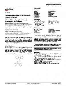
4. Performance evaluation and experimental results To evaluate the performance of the proposed algorithms, we have implemented the proposed methods along with the Thakur’s methods [24, 25] and the PITFALLS method [21, 22] on an IBM SP2 parallel machine. All algorithms were written in the single program multiple data (SPMD) programming paradigm with C 1 MPI codes. To get the experimental results, we have executed those programs for different kinds of kr R r and r R kr array redistribution with various array size N on a 64-node IBM SP2 parallel machine, where N [ {1.28M, 2.56M, 3.84M, 5.12M, 6.4M} and k [ {5, 25, 50, 100, N/64}. For a particular redistribution, all algorithms were executed 20 times. The mean time of the 20 tests was used as the time of an algorithm to perform the redistribution. Time was measured by using MPI_Wtime¼. The single-precision array was used for the test. The experimental results were shown in Figure 7 to Figure 11. In Figure 7 to Figure 11, the Krr represents the algorithms proposed in this paper. The Thakur and the PITFALLS represent the algorithms proposed in [24, 25] and [21,22], respectively. Figure 7 gives the execution time of these algorithms to perform BLOCK-CYCLIC(10) to BLOCK-CYCLIC(2) and BLOCK-CYCLIC(2) to BLOCK-CYCLIC(10) redistribution with various array size, where k 5 5. In Figure 7(a), the execution time of these three algorithms has the order T(Krr) , T(PITFALLS) , T(Thakur). From Figure 7(c), for the kr R r redistribution, we can see that the computation time of these three algorithms has the order Tcomp(Krr) , Tcomp(Thakur) , Tcomp(PITFALLS). For the PITFALLS method, a processor needs to find out all intersections between source and destination distribution with all other processors involved in the redistribution. Therefore, the PITFALLS method requires additional computation time at communication sets calculation. For the Thakur’s method, a processor needs to scan its local array elements once to determine the destination (source) processor for each block of array elements of size r in the local array. The Thakur’s method also requires additional computation time at communication sets calculation. However, for the Krr method, based on the packing/unpacking information derived from the kr R r redistribution, it can pack/unpack array elements to/from messages directly without calculating the communication sets. Therefore, the computation time of the Krr method is the lowest one among these three methods. For the same case, the communication time of these three algorithms has the order Tcomm(Krr) , Tcomm(PITFALLS) , Tcomm(Thakur). For the Krr method and the PITFALLS method, both methods use asynchronous communication schemes. The computation and the communication overheads can be overlapped. However, the Krr method unpacks any
Kluwer Journal @ats-ss10/data11/kluwer/journals/supe/v12n3art2
COMPOSED: 05/05/98 3:52 pm.
PG.POS. 17
SESSION: 43
270
CHING-HSIEN HSU AND YEH-CHING CHUNG
Figure 7. Performance of different algorithms to execute a BLOCK-CYCLIC(10) to BLOCK-CYCLIC(2) redistribution and vice versa with various array size (N 5 1.28Mbytes) on a 64-node SP2. (a) The kr R r redistribution. (b) The r R kr redistribution. (c) The computation time and the communication time of (a) and (b).
received messages in the receiving phase while the PITFALLS method unpacks messages in a specific order. Therefore, the communication time of the Krr method is less than or equal to that of the PITFALLS method. For the Thakur’s method, due to the algorithm design strateagy, it uses a synchronous communication scheme in the kr R r redistribution. In a synchronous communication scheme, the computation and the communication overheads can not be overlapped. Therefore, the Thakur’s method has higher communication overheads than those of the Krr method and the PITFALLS method. Figure 7(b) presents the exetution time of these algorithms for the r R kr redistribution. The execution time of these three algorithms has the order T(Krr) , T(Thakur) , T(PITFALLS). In Figure 7(c), for the r R kr redistribution, the computation time of these three algorithms have the order Tcomp(Krr) , Tcomp(Thakur) , Tcomp(PITFALLS). The reason is similar to that described for Figure 7(a).
Kluwer Journal @ats-ss10/data11/kluwer/journals/supe/v12n3art2
COMPOSED: 05/05/98 3:52 pm.
PG.POS. 18
SESSION: 43
ARRAY REDISTRIBUTION
271
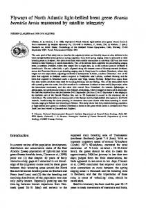
Figure 8. Performance of different algorithms to execute a BLOCK-CYCLIC(50) to BLOCK-CYCLIC(2) redistribution and vice versa with various array size (N 5 1.28M single precision) on a 64-node SP2. (a) The kr R r redistribution. (b) The r R kr redistribution. (c) The computation time and the communication time of (a) and (b).
For the communication time, the Thakur’s method and the Krr method have similar communication overheads and are less than that of the PITFALLS method. In the r R kr redistribution, all these three algorithms use asynchronous communication schemes. However, the Krr method and the Thakur’s method unpack any received message in the receiving phase while the PITFALLS method unpacks messages in a specific order. Therefore, the PITFALLS method has more communication overheads than those of the Krr method and the Thakur’s method. Figures 8, 9, and 10 are the cases when k is equal to 25, 50, and 100, respectively. From Figure 8 to Figure 10, we have similar observations as those described for Figure 7. Figure 11 gives the execution time of these algorithms to perform BLOCK to CYCLIC and vice versa redistribution with various array size. In this case, the value of k is equal to N/64. From Figure 11(a) and (b), we can see that the execution time of these three algorithms has the order T(Krr) , T(Thakur) ! T(PITFALLS) for both kr R r and r R kr redistribution. In Figure 11(c), for both kr R r and r R kr redistribution, the compu-
Kluwer Journal @ats-ss10/data11/kluwer/journals/supe/v12n3art2
COMPOSED: 05/05/98 3:52 pm.
PG.POS. 19
SESSION: 43
272
CHING-HSIEN HSU AND YEH-CHING CHUNG
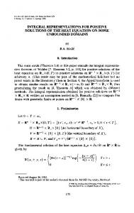
Figure 9. Performance of different algorithms to execute a BLOCK-CYCLIC(100) to BLOCK-CYCLIC(2) redistribution and vice versa with various array size (N 5 1.28M single precision) on a 64-node SP2. (a) The kr R r redistribution. (b) The r R kr redistribution. (c) The computation time and the communication time of (a) and (b).
tation time of theses three algorithms has the order Tcomp(Krr) , Tcomp(Thakur) ! Tcomp (PITFALLS). The PITFALLS method has very large computation time compared to those of the Krr method and the Thakur’s method. Th reason is that each processor needs to find out all intersections between source and destination distribution with all other processors in the PITFALLS method. The computation time of the PITFALLS method depends on the number of intersections. In this case, there are N/64 intersections between each source and destination processor. Therefore, a processor needs to compute N/64 3 64 intersections which demands a lot of computation time when N is large. For the communication overheads, we have similar observations as those described for Figure 7(b). From the above performance analysis and experimental results, we can see that the Krr method outperforms the Thakur’s method and the PITFALLS method for all test samples.
Kluwer Journal @ats-ss10/data11/kluwer/journals/supe/v12n3art2
COMPOSED: 05/05/98 3:52 pm.
PG.POS. 20
SESSION: 43
ARRAY REDISTRIBUTION
273
Figure 11. Performance of different algorithms to execute a BLOCK to CYCLIC redistribution and vice versa with various array size (N 5 1.28M single precision) on a 64-node SP2. (a) The BLOCK to CYCLIC redistribution. (b) The CYCLIC to BLOCK redistribution. (c) The computation time and the communication time of (a) and (b).
5. Conclusions Array redistribution is usually used in data-parallel programs to minimizing the run-time cost of performing data exchange among different processors. Since it is performed at run-time, efficient methods are required for array redistribution. In this paper, we have presented efficient algorithms for kr R r and r R kr redistribution. The most significant improvement of our algorithms is that a processor does not need to construct the send/ receive data sets for a redistribution. Based on the packing/unpacking information that derived from the kr R r and r R kr redistribution, a processor can pack/unpack array elements to (from) messages directly. To evaluate the performance of our methods, we have implemented our methods along with the Thakur’s method and the PITFALLS method on an IBM SP2 parallel machine. The experimental results show that our algorithms outperform the Thakur’s methods and the PITFALLS method. This result encourages us to use the proposed algorithms for array redistribution.
Kluwer Journal @ats-ss10/data11/kluwer/journals/supe/v12n3art2
COMPOSED: 05/05/98 3:52 pm.
PG.POS. 21
SESSION: 43
274
CHING-HSIEN HSU AND YEH-CHING CHUNG
Figure 10. Performance of different algorithms to execute a BLOCK-CYCLIC(200) to BLOCK-CYCLIC(2) redistribution and vice versa with various array size (N 5 1.28M single precision) on a 64-node SP2. (a) The kr R r redistribution. (b) The r R kr redistribution. (c) The computation time and the communication time of (a) and (b).
Acknowledgements The work of this paper was partially supported by NSC under contract NSC87-2213-E035-011.
References 1. S. Benkner. Handling block-cyclic distribution arrays in Vienna Fortran 90. In Proceeding of Intl. Conf. on Parallel Architectures and Compilation Techniques, Limassol, Cyprus, June 1995. 2. B. Chapman, P. Mehrotra, H. Moritsch, and H. Zima. Dynamic data distribution in Vienna Fortran. Proc. of Supercomputing’93, pp. 284–293. Nov. 1993. 3. S. Chatterjee, J. R. Gilbert, F. J. E. Long, R. Schreiber, and S.-H. Teng. Generating Local Address and Communication Sets for Data Parallel Programs. Journal of Parallel and Distributed Computing, vol. 26, pp. 72–84. 1995.
Kluwer Journal @ats-ss10/data11/kluwer/journals/supe/v12n3art2
COMPOSED: 05/05/98 3:52 pm.
PG.POS. 22
SESSION: 43
ARRAY REDISTRIBUTION
275
4. Y.-C Chung, C.-S Sheu and S.-W Bai. A Basic-Cycle Calculation Technique for Efficient Dynamic Data Redistribution. In Proceedings of Intl. Computer Symposium on Distributed Systems, pp. 137–144. Dec. 1996. 5. J. J. Dongarra, R. Van De Geijn, and D. W. Walker. A look at scalable dense linear algebra libraries. Technical Report ORNL/TM-12126 from Oak Ridge National Laboratory. Apr. 1992. 6. G. Fox, S. Hiranandani, K. Kennedy, C. Koelbel, U. Kremer, C.-W. Tseng, and M. Wu. Fortran-D Language Specification. Technical Report TR-91-170, Dept. of Computer Science. Rice University. Dec. 1991. 7. S. K. S. Gupta, S. D. Kaushik, C.-H. Huang, and P. Sadayappan. On the Generation of Efficient Data Communication for Distributed-Memory Machines. Proc. of Intl. Computing Symposium, pp. 504–513. 1992. 8. S. K. S. Gupta, S. D. Kaushik, C.-H. Huang, and P. Sadayappan. On Compiling Array Expressions for Efficient Execution on Distributed-Memory Machines. Journal of Parallel and Distributed Computing, vol. 32, pp. 155–172. 1996. 9. High Performance Fortran Forum. High Performance Fortran Language Specification(version 1.1). Rice University. November 1994. 10. S. Hiranandani, K. Kennedy, J. Mellor-Crammey, and A. Sethi. Compilation technique for block-cyclic distribution. In Proc. ACM Intl. Conf. on Supercomputing, pp. 392–403. July 1994. 11. Edgar T. Kalns, and Lionel M. Ni. Processor Mapping Technique Toward Efficient Data Redistribution. IEEE Transactions on Parallel and Distributed Systems, vol. 6, no. 12. December 1995. 12. E. T. Kalns and L. M. Ni, DaReL: A portable data redistribution library for distributed-memory machines. In Proceedings of the 1994 Scalable Parallel Libraries Conference II. Oct. 1994. 13. S. D. Kaushik, C. H. Huang, R. W. Johnson, and P. Sadayappan. An Approach to communication efficient data redistribution. In Proceeding of International Conf. on Supercomputing, pp. 364–373. July 1994. 14. S. D. Kaushik, C. H. Huang, J. Ramanujam, and P. Sadayappan. Multiphase array redistribution: Modeling and evaluation. In Proceeding of International Parallel processing Symposium, pp. 441–445. 1995. 15. S. D. Kaushik, C. H. Huang, and P. Sadayappan. Efficient Index Set Generation for Compiling HPF Array Statements on Distributed-Memory Machines. Journal of Parallel and Distributed Computing, vol. 38, pp. 237–247. 1996. 16. K. Kennedy, N. Nedeljkovic, and A. Sethi. Efficient address generation for block-cyclic distribution. In Proceeding of International Conf. on Supercomputing, pp. 180–184, Barcelona. July 1995. 17. P-Z. Lee and W. Y. Chen. Compiler techniques for determining data distribution and generating communication sets on distributed-memory multicomputers. 29th IEEE Hawaii Intl. Conf. on System Sciences, Maui, Hawaii. pp.537–546. Jan 1996. 18. Young Won Lim, Prashanth B. Bhat, and Viktor K. Prasanna. Efficient Algorithms for Block-Cyclic Redistribution of Arrays. Proceedings of the Eighth IEEE Symposium on Parallel and Distributed Processing, pp. 74–83. 1996. 19. Y. W. Lim, N. Park, and V. K. Prasanna. Efficient Algorithms for Multi-Dimensional Block-Cyclic Redistribution of Arrays. Proceedings of the 26th International Conference on Parallel Processing, pp. 234–241. 1997. 20. L. Prylli and B. Touranchean. Fast runtime block cyclic data redistribution on multiprocessors. Journal of Parallel and Distributed Computing, vol. 45, pp. 63–72. Aug. 1997. 21. S. Ramaswamy and P. Banerjee. Automatic generation of efficient array redistribution routines for distributed memory multicomputers. Frontier’95: The Fifth Symposium on the Frontiers of Massively Parallel Computation, pp. 342–349. Mclean, VA., Feb. 1995. 22. S. Ramaswamy, B. Simons, and P. Banerjee. Optimization for Efficient Array Redistribution on Distributed Memory Multicomputers. Journal of Parallel and Distributed Computing, vol. 38, pp. 217–228. 1996. 23. J. M. Stichnoth, D. O’Hallaron, and T. R. Gross. Generating communication for array statements: Design, implementation, and evaluation. Journal of Parallel and Distributed Computing, vol. 21, pp. 150–159. 1994.
Kluwer Journal @ats-ss10/data11/kluwer/journals/supe/v12n3art2
COMPOSED: 05/05/98 3:52 pm.
PG.POS. 23
SESSION: 43
276
CHING-HSIEN HSU AND YEH-CHING CHUNG
24. R. Thakur, A. Choudhary, and G. Fox. Runtime array redistribution in HPF programs. Proc. 1994 Scalable High Performance Computing Conf., pp. 309–316. May 1994. 25. Rajeev. Thakur, Alok. Choudhary, and J. Ramanujam. Efficient Algorithms for Array Redistribution. IEEE Transactions on Parallel and Distributed Systems, vol. 7, no. 6. June 1996. 26. A. Thirumalai and J. Ramanujam. HPF array statements: Communication generation and optimization. 3th workshop on Languages, Compilers and Run-time system for Scalable Computers, Troy. NY. May 1995. 27. V. Van Dongen, C. Bonello and C. Freehill. High Performance C - Language Specification Version 0.8.9. Technical Report CRIM-EPPP-94/04–12. 1994. 28. C. Van Loan. Computational Frameworks for the Fast Fourier Transform. SIAM, 1992. 29. David W. Walker, and Steve W. Otto. Redistribution of BLOCK-CYCLIC Data Distributions Using MPI. Concurrency: Practice and Experience, 8.9:707–728, Nov. 1996. 30. Akiyoshi Wakatani and Michael Wolfe. A New Approach to Array Redistribution: Strip Mining Redistribution. In Proceeding of Parallel Architectures and Languages Europe. July 1994. 31. Akiyoshi Wakatani and Michael Wolfe. Optimization of Array Redistribution for Distributed Memory Multicomputers. In Parallel Computing (submitted). 1994. 32. H. Zima, P. Brezany, B. Chapman, P. Mehrotra, and A. Schwald. Vienna Fortran - A Language Specification Version 1.1. ICASE Interim Report 21. ICASE NASA Langley Research Center, Hampton, Virginia 23665. March, 1992.
Kluwer Journal @ats-ss10/data11/kluwer/journals/supe/v12n3art2
COMPOSED: 05/05/98 3:52 pm.
PG.POS. 24
SESSION: 43


![AC2[R+,R] - Hindawi](https://m.moam.info/img/260x300/ac2rr-hindawi_5b5b550f097c47ff718b4589.jpg)
