GENERALIZED SURFACE PLASMON RESONANCE SENSORS ...

Progress In Electromagnetics Research, PIER 51, 139–152, 2005

GENERALIZED SURFACE PLASMON RESONANCE SENSORS USING METAMATERIALS AND NEGATIVE INDEX MATERIALS A. Ishimaru, S. Jaruwatanadilok, and Y. Kuga Box 352500, Department of Electrical Engineering University of Washington Seattle, Washington 98195, USA Abstract—Optical surface plasmon resonance sensors have been known for a long time. In this paper, we discuss the use of metamaterials to construct a surface plasmon sensor which can be used at microwave frequencies. We review the conditions for the existence of surface plasmon and the use of the forward and backward surface waves. A sharp dip in the reflection coefficient occurs when the propagation constant of the incident wave along the surface is nearly equal to the propagation constant of the plasmon surface wave and may be used to probe bulk material characteristics or to determine metamaterial characteristics. Numerical examples are given to illustrate the basic characteristics. 1 Introduction 2 Formulations for a Resonance Sensor

Generalized

Surface

Plasmon

3 Conventional Optical Surface Plasmon Resonance Sensor 4 Surface Plasmon for Metamaterials 5 Surface Plasmon Resonance Sensor 6 Surface Plasmon Sensor with Gap 7 Frequency Dependence and Effects of Loss 8 Conclusions Acknowledgment References

140

Ishimaru, Jaruwatanadilok, and Kuga

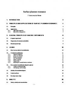
1. INTRODUCTION The phenomenon of surface plasmon resonance has been known for a long time and has been used for chemical sensors and remote sensing systems [1]. It makes use of a prism and a thin metal layer deposited upon the prism. The p-polarized (TM) reflected light exhibits a sharp dip at the incident angle where the propagation constant along the surface closely matches the propagation constant of the surface plasmon between the metal and the bulk material. This resonance occurs due to the negative dielectric constant of the metal, such as gold or silver, at optical frequencies. In this paper, we explore the use of the NIM (Negative Index Materials), and more generally metamaterials, to produce the surface plasmon resonance at microwave frequencies. Metamaterials and NIM have attracted considerable attention in recent years [2–6], and the surface plasmon on NIM has also been discussed [7, 8]. We first discuss the surface wave (surface plasmon) modes between metamaterials and the dielectric. This requires the study of all wave types which may exist between the medium with arbitrary ε and µ and the ordinary medium. We discuss the classification of wave types. In particular, we discuss the regimes in the µ-ε diagram where the forward and backward surface waves exist. These regimes give rise to the surface waves, and the reflection coefficient exhibits a sharp dip at this particular angle, similar to the conventional optical surface plasmon resonance sensor. We clarify the relationships between the p (TM) and s (TE) polarizations. We examine the fields inside NIM, and the interesting behaviors of the Poynting vectors, which point to the opposite direction in the inside and outside of NIM. We discuss the angular and frequency sensitivities of this phenomenon and the effect of the loss and possible difficulties in implementation for practical applications. 2. FORMULATIONS FOR A GENERALIZED SURFACE PLASMON RESONANCE SENSOR Let us consider the layered structure shown in Fig. 1. A plane wave is incident from the medium 1 with ε1 and µ1 on the layer with ε2 and µ2 bounded by the medium 3 with ε3 and µ3 . Here ε and µ are relative permittivity and relative permeability normalized to free space εo and µo . The reflection coefficient R is well known [9] R=

A + B/Z3 − Z1 (C + D/Z3 ) A + B/Z3 + Z1 (C + D/Z3 )

(1)

Progress In Electromagnetics Research, PIER 51, 2005

R

z

θ

141

θ

ε1 µ1 , n12 = ε1µ1 x

d

ε 2 µ 2 , n22 = ε 2 µ 2 ε 3 µ 3 , n32 = ε 3 µ 3

Figure 1. Geometry of layered metamaterials. where A = D = cos kz2 d, B = jZ2 sin kz2 d, C =

kzi =

j sin kz2 d Z2

ki2 − (ki sin θ1 )2 , i = 1, 2, 3, ki = ko ni

ko = ω/c is the free space wave number  kzi   for p-polarization (Ex , Ez , Hy )  ωεo εi Zi = ωµo µi   for s-polarization (Hx , Hz , Ey )  kzi In this formulation, both εi and µi are complex. However, for a passive medium, we require, using exp(jωt) time dependence, Im(εi ) < 0 Im(µi ) < 0 Im(ni ) < 0 Im(kzi ) < 0 Re µi /εi > 0

(2)

In the following sections, we examine (1) for metamaterials and discuss its physical meanings. 3. CONVENTIONAL OPTICAL SURFACE PLASMON RESONANCE SENSOR Before we discuss NIM surface plasmon resonance, we give a brief review of the conventional optical sensor making use of the surface

142


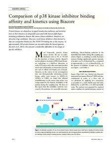
plasmon resonance. A prism with ε1 and µ1 has a thin metallic layer with ε2 and µ2 , and this is inserted into a medium whose characteristics are to be determined. A p-polarized (TM) plane wave is incident from the plasma and the reflected wave is measured as functions of angle and frequency. For the conventional surface plasmon sensor, µ1 = µ2 = µ3 = 1. R

θ

ε1 prism

d

x gold or silver ε 2 bulk material ε 3

Figure 2. Surface plasmon geometry and the reflection coefficient plot of a conventional optical surface plasmon sensor ε1 = 2.25, ε2 = −10 − j0.1, ε3 = 1.75, µ1 = µ2 = µ3 = 1, d = 0.05 µm, λ = 0.6 µm. As an example, Fig. 2 shows a reflection coefficient R as a function of the incident angle. The metal layer, normally gold or silver, has a negative real part of ε2 at optical frequency. There are two angles θc and θpl in Fig. 1, which are closely related to the material characteristics. The angle θc is close to the total reflection angle between the medium 1 and medium 3, n1 sin θc = n3

(3)

The angle θpl is when the propagation constant of the incident wave along the surface is close to the propagation constant of the surface plasmon between medium 2 and 3, ko n1 sin θpl = ksp = ko S

(4)

The propagation constant of the surface wave is well known [1, 9] S2 =

ε2 ε3 ε2 + ε3

(5)

The sharp dip at θpl is used to determine ε3 , and there is no surface plasmon for s-polarization.


143

4. SURFACE PLASMON FOR METAMATERIALS We now generalize the conventional plasmon sensor in Section 3 to include the metamaterials with arbitrary ε and µ. To do this, we first examine the plasmon which exists between the medium with εd and µd and the metamaterial with εm and µm .

z

ε d > 0, µ d > 0 x

ε m µ m (metamaterial) Figure 3. Surface wave along x between two media. For p-polarization, we have Hyd = exp{−jko Cd z − jko Sx} for z > 0 Hym = exp{+jko Cm z − jko Sx} for z < 0

(6)

Satisfying the boundary condition that Ex and Hy be continuous at z = 0, we get Cd Cm + =0 (7) εd εm From this, we get the propagation constant S S2 =

n2d ε2m − n2m ε2d ε2m − ε2d

(8)

The above equation is for the p-polarized (TM) wave. But it can be shown that for the s-polarized (TE) wave, S is given by switching ε and µ n2 µ2 − n2m µ2d (9) S2 = d m µ2m − µ2d Here, the medium for z > 0 is assumed to be an ordinary medium with εd > 0 and µd > 0, and this may be called the “double positive medium” (DPO) as opposed to the “double negative medium” (DNG) with ε < 0 and µ < 0. Here, we assume that the losses are negligibly small and therefore ε and µ are real with negligible negative imaginary parts.

144


First, we note that in order to have the surface wave, we require S 2 > n2d

(10)

Furthermore, the choice of the sign for S needs to be determined by Eq. (7). Also, we need to choose S such that Im(Cd ) < 0 Im(Cm ) < 0.

(11)

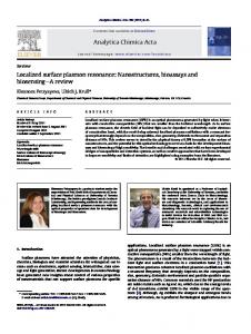
In Fig. 4, we show the regions in µ-ε diagram where S 2 > n2d . 3

2

µm /µd

1

SW+

0

-1

-2 S SW-3 -3

-2

-1

0

1

2

3

ε m/ε d

Figure 4. Forward (SW+) and backward (SW−) surface plasmons. The curve in the third quadrant is given by (µm εm )/(µd εd ) = −1. Eqs. (7), (8) and the conditions (11) give two regions where the surface wave propagates in the forward (+x) direction (SW+), and in the backward (−x) direction (SW−). Note that Fig. 4 is for p-polarization. For s-polarization, ε and µ are switched and the horizontal axis is µm /µd and the vertical axis is εm /εd , and all discussion on SW+ and SW− is unchanged. The fields inside and outside the metamaterial show that in the region of SW− in Fig. 4, the phase velocities along the surface in the medium (εd , µd ) and the NIM (εm < 0, µm < 0) are in the same direction, but the Poynting vectors


145

and the group velocities along the surface in the medium (εd , µd ) and in NIM are in the opposite direction. 5. SURFACE PLASMON RESONANCE SENSOR Let us now consider the structure shown in Fig. 5.

R

z

θ

d

θ

ε 2 µ2

ε 1 µ1 metamaterial

ε 3 µ3

x

Figure 5. Metamaterial with ε2 and µ2 is placed under the prism with ε1 and µ1 = 1 and the dielectric material with ε3 and µ3 = 1. The surface plasmon propagation constant S between the medium 2 and 3 is given by Eq. (8) or (9). The dip in the reflection coefficient should occur in the regions of SW+ and SW− in Fig. 4 with εm = ε2 , µm = µ2 , and εd = ε3 , µd = µ3 . Furthermore, in order to have the plasmon resonance sensor, we need to have a total reflection requiring n 1 > n3

(12)

and the dip occurs at the angle θpl where n1 sin θpl = S

(13)

Combining with Eq. (10), we need to have n23 < S 2 < n21

(14)

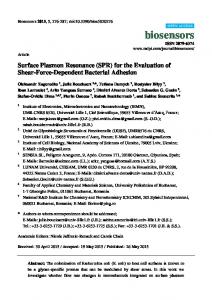
This is shown in Fig. 6. The reflection coefficients as functions of incident angle θ are shown in Fig. 7. The results are for the following cases: Case A : ε2 = −1.5 − 0.001j µ2 = −2 Case B : ε2 = −4.5 − 0.001j µ2 = 1 Case C : ε2 = −0.66 − 0.001j µ2 = −2 d = 0.3λo

(15)

Note that the plasmon does not exist in Case C, and there is no dip in reflection coefficient.

146

Ishimaru, Jaruwatanadilok, and Kuga 3 2 1

*

µm/µd

Case B 0 -1 Case C -2 -3 -3

Case A * * -2

-1

0

1

2

3

ε m/ε d

Figure 6. Surface plasmon resonance sensor ε1 = 5, ε3 = 2, µ1 = µ3 = 1. Surface waves can exist in the shaded regions. Case B

Case A 1

1

0.9

0.95

0.8

0.9

0.7

0.85 0.6

0.8 0.5

0.75

0.4 0.3

0.7

0.2 0

0.65 0

20

40 60 Incident angle (degrees)

80

20


Case C 1

0.8

0.6

0.4

0.2

0 0

20


80

Figure 7. Reflection coefficient at A, B, and C.

80


147

6. SURFACE PLASMON SENSOR WITH GAP Next we consider the structure in Fig. 8.

θ

d

θ

ε 1 µ1

ε 2 µ2 gap

metamaterial ε 3 µ 3

x

Figure 8. Structure with gap. Here, we use ε1 = 5, ε2 = 2, µ1 = µ2 = 1. Figure 9 shows the cases A, B, and C where ε3 and µ3 are metamaterials shown in Eq. (15). Note that there is a sharp dip for Case A and B, but not for Case C. This configuration may be convenient to determine the characteristics of a metamaterial. 7. FREQUENCY DEPENDENCE AND EFFECTS OF LOSS It is known that metamaterials are often highly dispersive and lossy. Therefore, it is important to examine the frequency dependence of the surface plasmon sensor. However, the frequency characteristics of metamaterials depend on how the material is made. In particular, there appears to be no general formula for µ(ω), even though the Lorentz model and Drude model have been used [6]. Here we consider a narrow band approximation where |∆ω| = |ω − ωo | ωo . Noting the group refractive index ng is given by ng =

∂ (nω), ∂ω

(16)

we get, in narrow band approximation, n(ω) = n(ωo ) + [ng (ωo ) − n(ωo )]

∆ω ωo

where, in general, both and n(ωo ) are ng (ωo ) are complex.

(17)

148

Ishimaru, Jaruwatanadilok, and Kuga Case B

Case A

1.005

1 0.9

1

0.8

0.995

0.7

0.99

0.6

0.985

0.5

0.98

0.4

0.975

0.3

0.97

0.2 0

0.965 0

20


80

20


80

Case C 1

0.8

0.6

0.4

0.2

0 0

20


80

Figure 9. Reflection coefficient as a function of incident angle in gap structure. Similarly, we can approximate ε and µ as ∆ω ωo ∆ω µ(ω) = µ(ωo ) + δm ωo ε(ω) = ε(ωo ) + δe

where δe =

∂ε ∂ω ωo ωo

(18)

and δm =

∂µ ∂ω ωo ωo .

1 ng (ωo ) = n(ωo ) 1 + 2

We then get

δe δm + ε(ωo ) µ(ωo )

(19)

Note that for NIM, n(ωo ), ε(ωo ), and µ(ωo ) are negative, but δe , δm , and ng are positive. As an example, we take Case A and let δe = δm = δ. Figure 10


149

1 0.95 0.9 0.85 0.8 =0 =0.01 =0.001

0.75 0.7 68

Figure 10. coefficient.

69 70 71 Incident angle (degrees)

72

Effect of the frequency dependence to the reflection

1

0.9

0.8

0.7

0.6

Case (1) Case (2) Case (3)

0.5

0.4 66

67

68

69 70 71 Incident angle (degrees)

72

73

74

Figure 11. The effect of loss. (1) ε2 = −1.5 − 0.001j, µ2 = −2, (2) ε2 = −1.5 − 0.001j, µ2 = −2 − 0.01j, (3) ε2 = −1.5 − 0.001j, µ2 = −2 − 0.001j.

150


shows the variation of the dip of the reflection coefficient for a small change of δ. Next, we consider the effect of loss. For Case A, ε2 and µ2 are given in Eq. (15). We calculate and show the effect of loss in Fig. 11. Note that increased loss broadens the dip as expected. 8. CONCLUSIONS We present the use of metamaterials for plasmon resonance sensors at microwave frequencies. The conditions for the existence of forward and backward surface waves are clarified using the µ-ε diagram. Metamaterial surface plasmon sensors may be useful for remote sensing of material characteristics or for determining metamaterial characteristics. This paper deals with a surface plasmon sensor making use of isotropic and homogeneous metamaterials. However, there are some practical issues, including the questions of how to construct such metamaterials, and what are the effects of anisotropic characteristics. Since most metamaterials are known to be highly dispersive and lossy, the sensitivities need to be carefully studied. It is also important to investigate how to construct practical broadband, low-loss metamaterials. ACKNOWLEDGMENT This work was supported by the National Science Foundation (ECS990 8849). REFERENCES 1. Jorgenson, R. C. and S. S. Yee, “A fiber-optic chemical sensor based on surface plasmon resonance,” Sensors and Actuators B, Vol. 12, 213–220, 1993. 2. Veselago, V. G., “The electrodynamics of substances with simultaneously negative values of ε and µ,” Sov. Phy. Usp., Vol. 10, No. 4, 509–514, Jan.–Feb. 1968. 3. Pendry, J. B., A. J. Holden, D. J. Robbins, and W. J. Stewart, “Magnetism from conductors and enhanced nonlinear phenomena,” IEEE Trans. Microwave Theory and Techniques, Vol. 47, No. 11, 2075–2084, November 1999. 4. Smith, D. R., W. J. Padilla, D. C. Vier, S. C. Nemat-Nasser, and S. Schultz, “Composite medium with simultaneously negative


5. 6.

7. 8.

9.

151

permeability and permittivity,” Phys. Rev. Lett., Vol. 84, No. 18, 4184–4187, May 2000. Pendry, J. B., “Negative refraction makes a perfect lens,” Phy. Rev. Lett., Vol. 85, No. 18, 3966–3969, October 2000. Ziolkowski, R. W. and E. Heyman, “Wave propagation in media having negative permittivity and permeability,” Phy. Rev. E, Vol. 64, No. 5, 056625, 2001. Ruppin, R., “Surface polaritons of a left-handed medium,” Phy. Lett. A, Vol. 277, 61–64, 2000. Caloz, C., A. Sanada, and T. Itoh, “Surface plasmons at the interface between right-handed and left-handed 2D metamaterials,” IEEE-APS International Symposium, Vol. 3, Columbus, OH, June 2003. Ishimaru, A., Electromagnetic Wave Propagation, Radiation, and Scattering, Prentice Hall, 1991.

Akira Ishimaru is professor emeritus of electrical engineering at the University of Washington. He is the author of the books, Wave Propagation and Scattering in Random Media (Academic Press, 1978; IEEE Press-Oxford University Press Classic Reissue, 1997) and Electromagnetic Wave Propagation, Radiation, and Scattering (Prentice Hall, 1991). He is a Fellow of the IEEE, the Optical Society of America, the Acoustical Society of America, and the Institute of Physics, United Kingdom. He is a member of the National Academy of Engineering. He is the recipient of the 1999 IEEE Heinrich Hertz Medal and the 1999 URSI Dellinger Gold Medal. In 2000, he received the IEEE Third Millennium Medal. Sermsak Jaruwatanadilok received his B.E. degree from King Mongkut’s Institute of Technology, Ladkrabang, Thailand in 1994, M.S. degree from Texas A&M University, College Station, Texas, USA in 1997, and Ph.D. degree from University of Washington, Seattle, USA in 2003. He is now a research associate at the University of Washington, Seattle. His research interest lies in the area of remote sensing and waves in random media. Yasuo Kuga is a Professor of Electrical Engineering at the University of Washington. He received his B.S., M.S., and Ph.D. degrees from the University of Washington, Seattle in 1977, 1979, and 1983, respectively. From 1983 to 1988, he was a Research Assistant Professor of Electrical Engineering at the University of Washington. From 1988 to 1991, he was an Assistant Professor of Electrical Engineering and Computer

152


Science at The University of Michigan. Since 1991, he is with the University of Washington. He was an Associate Editor of Radio Science (1993–1996) and IEEE Trans. Geoscience and Remote Sensing (1996– 2000). He was elected to IEEE Fellow in 2004. His research interests are in the areas of microwave and millimeter-wave remote sensing, high frequency devices and materials, and optics.