Inducing Sound Segment Differences using Pair Hidden Markov Models
Martijn Wieling Alfa-Informatica University of Groningen
[email protected]
Therese Leinonen Alfa-Informatica University of Groningen
[email protected]
Abstract
consonants and vowels, but treat e.g. all the vowel differences as the same. Ignoring the special treatment of vowels vs. consonants, the techniques regard segments in a binary fashion—as alike or different—in spite of the overwhelming consensus that some sounds are much more alike than others. There have been many attempts to incorporate more sensitive segment differences, which do not necessarily perform worse in validation, but they fail to show significant improvement (Heeringa, 2004).
Pair Hidden Markov Models (PairHMMs) are trained to align the pronunciation transcriptions of a large contemporary collection of Dutch dialect material, the GoemanTaeldeman-Van Reenen-Project (GTRP, collected 1980–1995). We focus on the question of how to incorporate information about sound segment distances to improve sequence distance measures for use in dialect comparison. PairHMMs induce segment distances via expectation maximisation (EM). Our analysis uses a phonologically comparable subset of 562 items for all 424 localities in the Netherlands. We evaluate the work first via comparison to analyses obtained using the Levenshtein distance on the same dataset and second, by comparing the quality of the induced vowel distances to acoustic differences.
1
John Nerbonne Alfa-Informatica University of Groningen
[email protected]
Introduction
Dialectology catalogues the geographic distribution of the linguistic variation that is a necessary condition for language change (Wolfram and SchillingEstes, 2003), and is sometimes successful in identifying geographic correlates of historical developments (Labov, 2001). Computational methods for studying dialect pronunciation variation have been successful using various edit distance and related string distance measures, but unsuccessful in using segment differences to improve these (Heeringa, 2004). The most successful techniques distinguish
Instead of using segment distances as these are (incompletely) suggested by phonetic or phonological theory, we can also attempt to acquire these automatically. Mackay and Kondrak (2005) introduce Pair Hidden Markov Models (PairHMMs) to language studies, applying them to the problem of recognising “cognates” in the sense of machine translation, i.e. pairs of words in different languages that are similar enough in sound and meaning to serve as translation equivalents. Such words may be cognate in the sense of historical linguistics, but they may also be borrowings from a third language. We apply PairHMMs to dialect data for the first time in this paper. Like Mackay and Kondrak (2005) we evaluate the results both on a specific task, in our case, dialect classification, and also via examination of the segment substitution probabilities induced by the PairHMM training procedures. We suggest using the acoustic distances between vowels as a probe to explore the segment substitution probabilities induced by the PairHMMs. Naturally, this validation procedure only makes sense if dialects are using acoustically more similar sounds in their variation, rather than, for example,
48 Proceedings of Ninth Meeting of the ACL Special Interest Group in Computational Morphology and Phonology, pages 48–56, c Prague, June 2007. 2007 Association for Computational Linguistics
randomly varied sounds. But why should linguistic and geographic proximity be mirrored by frequency of correspondence? Historical linguistics suggests that sound changes propagate geographically, which means that nearby localities should on average share the most changes. In addition some changes are convergent to local varieties, increasing the tendency toward local similarity. The overall effect in both cases strengthens the similarity of nearby varieties. Correspondences among more distant varieties are more easily disturbed by intervening changes and decreasing strength of propagation.
Leeuwarden Veendam
Urk
Aalsmeer
Putten
Oldenzaal
Utrecht Delft
Middelburg
2
Coevorden
Material
Goirle Venlo
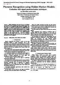
In this study the most recent Dutch dialect data source is used: data from the Goeman-TaeldemanVan Reenen-project (GTRP; Goeman and Taeldeman, 1996). The GTRP consists of digital transcriptions for 613 dialect varieties in the Netherlands (424 varieties) and Belgium (189 varieties), gathered during the period 1980–1995. For every variety, a maximum of 1876 items was narrowly transcribed according to the International Phonetic Alphabet. The items consisted of separate words and word groups, including pronominals, adjectives and nouns. A more detailed overview of the data collection is given in Taeldeman and Verleyen (1999). Since the GTRP was compiled with a view to documenting both phonological and morphological variation (De Schutter et al., 2005) and our purpose here is the analysis of variation in pronunciation, many items of the GTRP are ignored. We use the same 562 item subset as introduced and discussed in depth by Wieling et al. (2007). In short, the 1876 item word list was filtered by selecting only single word items, plural nouns (the singular form was preceded by an article and therefore not included), base forms of adjectives instead of comparative forms and the first-person plural verb instead of other forms. We omit words whose variation is primarily morphological as we wish to focus on pronunciation. Because the GTRP transcriptions of Belgian varieties are fundamentally different from transcriptions of Netherlandic varieties (Wieling et al., 2007), we will focus our analysis on the 424 varieties in the Netherlands. The geographic distribution of these
49
Figure 1. Distribution of GTRP localities. varieties is shown in Figure 1. Furthermore, note that we will not look at diacritics, but only at the phonetic symbols (82 in total).
3
The Pair Hidden Markov Model
In this study we will use a Pair Hidden Markov Model (PairHMM), which is essentially a Hidden Markov Model (HMM) adapted to assign similarity scores to word pairs and to use these similarity scores to compute string distances. In general an HMM generates an observation sequence (output) by starting in one of the available states based on the initial probabilities, going from state to state based on the transition probabilities while emitting an output symbol in each state based on the emission probability of that output symbol in that state. The probability of an observation sequence given the HMM can be calculated by using well known HMM algorithms such as the Forward algorithm and the Viterbi algorithms (e.g., see Rabiner, 1989). The only difference between the PairHMM and the HMM is that it outputs a pair of symbols instead of only one symbol. Hence it generates two (aligned) observation streams instead of one. The PairHMM was originally proposed by Durbin et al. (1998) and has successfully been used for aligning
Figure 2. Pair Hidden Markov Model. Image courtesy of Mackay and Kondrak (2005). biological sequences. Mackay and Kondrak (2005) adapted the algorithm to calculate similarity scores for word pairs in orthographic form, focusing on identifying translation equivalents in bilingual corpora. Their modified PairHMM has three states representing the basic edit operations: a substitution state (M), a deletion state (X) and an insertion state (Y). In the substitution state two symbols are emitted, while in the other two states a gap and a symbol are emitted, corresponding with a deletion and an insertion, respectively. The model is shown in Figure 2. The four transition parameters are specified by λ, δ, ε and τ . There is no explicit start state; the probability of starting in one of the three states is equal to the probability of going from the substitution state to that state. In our case we use the PairHMM to align phonetically transcribed words. A possible alignment (including the state sequence) for the two observation streams [mO@lk@] and [mEl@k] (Dutch dialectal variants of the word ‘milk’) is given by: m m M
O E M
@ X
l l M
@ Y
k k M
@ X
We have several ways to calculate the similarity score for a given word pair when the transition and emission probabilities are known. First, we can use the Viterbi algorithm to calculate the probability of the best alignment and use this probability as a sim-
50
ilarity score (after correcting for length; see Mackay and Kondrak, 2005). Second, we can use the Forward algorithm, which takes all possible alignments into account, to calculate the probability of the observation sequence given the PairHMM and use this probability as a similarity score (again corrected for length; see Mackay, 2004 for the adapted PairHMM Viterbi and Forward algorithms). A third method to calculate the similarity score is using the log-odds algorithm (Durbin et al., 1998). The log-odds algorithm uses a random model to represent how likely it is that a pair of words occur together while they have no underlying relationship. Because we are looking at word alignments, this means an alignment consisting of no substitutions but only insertions and deletions. Mackay and Kondrak (2005) propose a random model which has only insertion and deletion states and generates one word completely before the other, e.g. m O @ l k @ m E l @ k X X X X X X Y Y Y Y Y The model is described by the transition probability η and is displayed in Figure 3. The emission probabilities can be either set equal to the insertion and deletion probabilities of the word similarity model (Durbin et al., 1998) or can be specified separately based on the token frequencies in the data set (Mackay and Kondrak, 2005). The final log-odds similarity score of a word pair is calculated by dividing the Viterbi or Forward probability by the probability generated by the random model, and subsequently taking the logarithm of this value. When using the Viterbi algorithm the regular log-odds score is obtained, while using the Forward algorithm yields the Forward log-odds score (Mackay, 2004). Note that there is no need for additional normalisation; by dividing two models we are already implicitly normalising. Before we are able to use the algorithms described above, we have to estimate the emission probabilities (i.e. insertion, substitution and deletion probabilities) and transition probabilities of the model. These probabilities can be estimated by using the Baum-Welch expectation maximisation algorithm (Baum et al., 1970). The Baum-Welch algo-
We do not normalise the Levenshtein distance measurement for length, because Heeringa et al. (2006) showed that results based on raw Levenshtein distances are a better approximation of dialect differences as perceived by the dialect speakers than results based on the normalised Levenshtein distances. Finally, all substitutions, insertions and deletions have the same weight.
5
Figure 3. Random Pair Hidden Markov Model. Image courtesy of Mackay and Kondrak (2005). rithm iteratively reestimates the transition and emission probabilities until a local optimum is found and has time complexity O(T N 2 ), where N is the number of states and T is the length of the observation sequence. The Baum-Welch algorithm for the PairHMM is described in detail in Mackay (2004). 3.1
Calculating dialect distances
When the parameters of the complete model have been determined, the model can be used to calculate the alignment probability for every word pair. As in Mackay and Kondrak (2005) and described above, we use the Forward and Viterbi algorithms in both their regular (normalised for length) and log-odds form to calculate similarity scores for every word pair. Subsequently, the distance between two dialectal varieties can be obtained by calculating all word pair scores and averaging them.
4
The Levenshtein distance
The Levenshtein distance was introduced by Kessler (1995) as a tool for measuring linguistic distances between language varieties and has been successfully applied in dialect comparison (Nerbonne et al., 1996; Heeringa, 2004). For this comparison we use a slightly modified version of the Levenshtein distance algorithm, which enforces a linguistic syllabicity constraint: only vowels may match with vowels, and consonants with consonants. The specific details of this modification are described in more detail in Wieling et al. (2007).
51
Results
To obtain the best model probabilities, we trained the PairHMM with all data available from the 424 Netherlandic localities. For every locality there were on average 540 words with an average length of 5 tokens. To prevent order effects in training, every word pair was considered twice (e.g., wa − wb and wb − wa ). Therefore, in one training iteration almost 100 million word pairs had to be considered. To be able to train with these large amounts of data, a parallel implementation of the PairHMM software was implemented. After starting with more than 6700 uniform initial substitution probabilities, 82 insertion and deletion probabilities and 5 transition probabilities, convergence was reached after nearly 1500 iterations, taking 10 parallel processors each more than 10 hours of computation time. In the following paragraphs we will discuss the quality of the trained substitution probabilities as well as comment on the dialectological results obtained with the trained model. 5.1
Trained substitution probabilities
We are interested both in how well the overall sequence distances assigned by the trained PairHMMs reveal the dialectological landscape of the Netherlands, and also in how well segment distances induced by the Baum-Welch training (i.e. based on the substitution probabilities) reflect linguistic reality. A first inspection of the latter is a simple check on how well standard classifications are respected by the segment distances induced. Intuitively, the probabilities of substituting a vowel with a vowel or a consonant with a consonant (i.e. same-type substitution) should be higher than the probabilities of substituting a vowel with a consonant or vice versa (i.e. different-type substitution). Also the probability of substituting a phonetic
symbol with itself (i.e. identity substitution) should be higher than the probability of a substitution with any other phonetic symbol. To test this assumption, we compared the means of the above three substitution groups for vowels, consonants and both types together. In line with our intuition, we found a higher probability for an identity substitution as opposed to same-type and different-type non-identity substitutions, as well as a higher probability for a same-type substitution as compared to a different-type substitution. This result was highly significant in all cases: vowels (all p0 s ≤ 0.020), consonants (all p0 s < 0.001) and both types together (all p0 s < 0.001). 5.2
Vowel substitution scores compared to acoustic distances
PairHMMs assign high probabilities (and scores) to the emission of segment pairs that are more likely to be found in training data. Thus we expect frequent dialect correspondences to acquire high scores. Since phonetic similarity effects alignment and segment correspondences, we hypothesise that phonetically similar segment correspondences will be more usual than phonetically remote ones, more specifically that there should be a negative correlation between PairHMM-induced segment substitution probabilities presented above and phonetic distances. We focus on segment distances among vowels, because it is straightforward to suggest a measure of distance for these (but not for consonants). Phoneticians and dialectologists use the two first formants (the resonant frequencies created by different forms of the vocal cavity during pronunciation) as the defining physical characteristics of vowel quality. The first two formants correspond to the articulatory vowel features height and advancement. We follow variationist practice in ignoring third and higher formants. Using formant frequencies we can calculate the acoustic distances between vowels. Because the occurrence frequency of the phonetic symbols influences substitution probability, we do not compare substitution probabilities directly to acoustic distances. To obtain comparable scores, the substitution probabilities are divided by the product of the relative frequencies of the two phonetic symbols used in the substitution. Since substitutions in-
52
volving similar infrequent segments now get a much higher score than substitutions involving similar, but frequent segments, the logarithm of the score is used to bring the respective scores into a comparable scale. In the program PRAAT we find Hertz values of the first three formants for Dutch vowels pronounced by 50 male (Pols et al., 1973) and 25 female (Van Nierop et al., 1973) speakers of standard Dutch. The vowels were pronounced in a /hVt/ context, and the quality of the phonemes for which we have formant information should be close to the vowel quality used in the GTRP transcriptions. By averaging over 75 speakers we reduce the effect of personal variation. For comparison we chose only vowels that are pronounced as monophthongs in standard Dutch, in order to exclude interference of changing diphthong vowel quality with the results. Nine vowels were used: /i, I, y, Y, E, a, A, O, u/. We calculated the acoustic distances between all vowel pairs as a Euclidean distance of the formant values. Since our perception of frequency is nonlinear, using Hertz values of the formants when calculating the Euclidean distances would not weigh F1 heavily enough. We therefore transform frequencies to Bark scale, in better keeping with human perception. The correlation between the acoustic vowel distances based on two formants in Bark and the logarithmical and frequency corrected PairHMM substitution scores is r = −0.65 (p < 0.01). But Lobanov (1971) and Adank (2003) suggested using standardised z-scores, where the normalisation is applied over the entire vowel set produced by a given speaker (one normalisation per speaker). This helps in smoothing the voice differences between men and women. Normalising frequencies in this way resulted in a correlation of r = −0.72 (p < 0.001) with the PairHMM substitution scores. Figure 4 visualises this result. Both Bark scale and z-values gave somewhat lower correlations when the third formant was included in the measures. The strong correlation demonstrates that the PairHMM scores reflect phonetic (dis)similarity. The higher the probability that vowels are aligned in PairHMM training, the smaller the acoustic distance between two segments. We conclude therefore that the PairHMM indeed aligns linguistically corresponding segments in accord with phonetic similar-
Figure 4. Predicting acoustic distances based on PairHMM scores. Acoustic vowel distances are calculated via Euclidean distance based on the first two formants measured in Hertz, normalised for speaker. r = −0.72 ity. This likewise confirms that dialect differences tend to be acoustically slight rather than large, and suggests that PairHMMs are attuned to the slight differences which accumulate locally during language change. Also we can be more optimistic about combining segment distances and sequence distance techniques, in spite of Heeringa (2004, Ch. 4) who combined formant track segment distances with Levenshtein distances without obtaining improved results. 5.3
Dialectological results
To see how well the PairHMM results reveal the dialectological landscape of the Netherlands, we calculated the dialect distances with the Viterbi and Forward algorithms (in both their normalised and log-odds version) using the trained model parameters. To assess the quality of the PairHMM results, we used the LOCAL INCOHERENCE measurement which measures the degree to which geographically close varieties also represent linguistically similar varieties (Nerbonne and Kleiweg, 2005). Just as Mackay and Kondrak (2005), we found the overall best performance was obtained using the logodds version of Viterbi algorithm (with insertion and deletion probabilities based on the token frequen-
53
cies). Following Mackay and Kondrak (2005), we also experimented with a modified PairHMM obtained by setting non-substitution parameters constant. Rather than using the transition, insertion and deletion parameters (see Figure 2) of the trained model, we set these to a constant value as we are most interested in the effects of the substitution parameters. We indeed found slightly increased performance (in terms of LOCAL INCOHERENCE) for the simplified model with constant transition parameters. However, since there was a very high correlation (r = 0.98) between the full and the simplified model and the resulting clustering was also highly similar, we will use the Viterbi log-odds algorithm using all trained parameters to represent the results obtained with the PairHMM method. 5.4 PairHMM vs. Levenshtein results The PairHMM yielded dialectological results quite similar to those of Levenshtein distance. The LOCAL INCOHERENCE of the two methods was similar, and the dialect distance matrices obtained from the two techniques correlated highly (r = 0.89). Given that the Levenshtein distance has been shown to yield results that are consistent (Cronbach’s α = 0.99) and valid when compared to dialect speakers judgements of similarity (r ≈ 0.7), this means in particular that the PairHMMs are detecting dialectal variation quite well. Figure 5 shows the dialectal maps for the results obtained using the Levenshtein algorithm (top) and the PairHMM algorithm (bottom). The maps on the left show a clustering in ten groups based on UPGMA (Unweighted Pair Group Method with Arithmetic mean; see Heeringa, 2004 for a detailed explanation). In these maps phonetically close dialectal varieties are marked with the same symbol. However note that the symbols can only be compared within a map, not between the two maps (e.g., a dialectal variety indicated by a square in the top map does not need to have a relationship with a dialectal variety indicated by a square in the bottom map). Because clustering is unstable, in that small differences in input data can lead to large differences in the classifications derived, we repeatedly added random small amounts of noise to the data and iteratively generated the cluster borders based on the
Figure 5. Dialect distances for Levenshtein method (top) and PairHMM method (bottom). The maps on the left show the ten main clusters for both methods, indicated by distinct symbols. Note that the shape of these symbols can only be compared within a map, not between the top and bottom maps. The maps in the middle show robust cluster borders (darker lines indicate more robust cluster borders) obtained by repeated clustering using random small amounts of noise. The maps on the right show for each locality a vector towards the region which is phonetically most similar. See section 5.4 for further explanation.
54
noisy input data. Only borders which showed up during most of the 100 iterations are shown in the map. The maps in the middle show the most robust cluster borders; darker lines indicate more robust borders. The maps on the right show a vector at each locality pointing in the direction of the region it is phonetically most similar to. A number of observations can be made on the basis of these maps. The most important observation is that the maps show very similar results. For instance, in both methods a clear distinction can be seen between the Frisian varieties (north) and their surroundings as well as the Limburg varieties (south) and their surroundings. Some differences can also be observed. For instance, at first glance the Frisian cities among the Frisian varieties are separate clusters in the PairHMM method, while this is not the case for the Levenshtein method. Since the Frisian cities differ from their surroundings a great deal, this point favours the PairHMM. However, when looking at the deviating vectors for the Frisian cities in the two vector maps, it is clear that the techniques again yield similar results. Note that a more detailed description of the results using the Levenshtein distance on the GTRP data can be found in Wieling et al. (2007). Although the PairHMM method is much more sophisticated than the Levenshtein method, it yields very similar results. This may be due to the fact that the data sets are large enough to compensate for the lack of sensitivity in the Levenshtein technique, and the fact that we are evaluating the techniques at a high level of aggregation (average differences in 540-word samples).
6
Discussion
The present study confirms Mackay and Kondrak’s (2004) work showing that PairHMMs align linguistic material well and that they induce reasonable segment distances at the same time. We have extended that work by applying PairHMMs to dialectal data, and by evaluating the induced segment distances via their correlation with acoustic differences. We noted above that it is not clear whether the dialectological results improve on the simple Levenshtein measures, and that this may be due to the level of aggregation and the large sample sizes. But we would also like
55
to test PairHMMs on a data set for which more sensitive validation is possible, e.g. the Norwegian set for which dialect speakers judgements of proximity is available (Heeringa et al., 2006); this is clearly a point at which further work would be rewarding. At a more abstract level, we emphasise that the correlation between acoustic distances on the one hand and the segment distances induced by the PairHMMs on the other confirm both that alignments created by the PairHMMs are linguistically responsible, and also that this linguistic structure influences the range of variation. The segment distances induced by the PairHMMs reflect the frequency with which such segments need to be aligned in Baum-Welch training. It would be conceivable that dialect speakers used all sorts of correspondences to signal their linguistic provenance, but they do not. Instead, they tend to use variants which are linguistically close at the segment level. Finally, we note that the view of diachronic change as on the one hand the accumulation of changes propagating geographically, and on the other hand as the result of a tendency toward local convergence suggests that we should find linguistically similar varieties nearby rather than further away. The segment correspondences PairHMMs induce correspond to those found closer geographically. We have assumed a dialectological perspective here, focusing on local variation (Dutch), and using similarity of pronunciation as the organising variationist principle. For the analysis of relations among languages that are further away from each other— temporally and spatially—there is substantial consensus that one needs to go beyond similarity as a basis for postulating grouping. Thus phylogenetic techniques often use a model of relatedness aimed not at similarity-based grouping, but rather at creating a minimal genealogical tree. Nonetheless similarity is a satisfying basis of comparison at more local levels.
Acknowledgements We are thankful to Greg Kondrak for providing the source code of the PairHMM training and testing algorithms. We thank the Meertens Instituut for making the GTRP data available for research and espe-
cially Boudewijn van den Berg for answering our questions regarding this data. We would also like to thank Vincent van Heuven for phonetic advice and Peter Kleiweg for providing support and the software we used to create the maps.
Wesley Mackay and Grzegorz Kondrak. 2005. Computing word similarity and identifying cognates with Pair Hidden Markov Models. In Proceedings of the 9th Conference on Computational Natural Language Learning (CoNLL), pages 40–47, Morristown, NJ, USA. Association for Computational Linguistics.
References
Wesley Mackay. 2004. Word similarity using Pair Hidden Markov Models. Master’s thesis, University of Alberta.
Patti Adank. 2003. Vowel normalization - a perceptualacoustic study of Dutch vowels. Wageningen: Ponsen & Looijen. Leonard E. Baum, Ted Petrie, George Soules, and Norman Weiss. 1970. A maximization technique occurring in the statistical analysis of probabilistic functions of Markov Chains. The Annals of Mathematical Statistics, 41(1):164–171. Georges De Schutter, Boudewijn van den Berg, Ton Goeman, and Thera de Jong. 2005. Morfologische atlas van de Nederlandse dialecten - deel 1. Amsterdam University Press, Meertens Instituut - KNAW, Koninklijke Academie voor Nederlandse Taal- en Letterkunde. Richard Durbin, Sean R. Eddy, Anders Krogh, and Graeme Mitchison. 1998. Biological Sequence Analysis : Probabilistic Models of Proteins and Nucleic Acids. Cambridge University Press, July. Ton Goeman and Johan Taeldeman. 1996. Fonologie en morfologie van de Nederlandse dialecten. een nieuwe materiaalverzameling en twee nieuwe atlasprojecten. Taal en Tongval, 48:38–59.
John Nerbonne and Peter Kleiweg. 2005. Toward a dialectological yardstick. Accepted for publication in Journal of Quantitative Linguistics. John Nerbonne, Wilbert Heeringa, Erik van den Hout, Peter van der Kooi, Simone Otten, and Willem van de Vis. 1996. Phonetic distance between Dutch dialects. In Gert Durieux, Walter Daelemans, and Steven Gillis, editors, CLIN VI: Proc. from the Sixth CLIN Meeting, pages 185–202. Center for Dutch Language and Speech, University of Antwerpen (UIA), Antwerpen. Louis C. W. Pols, H. R. C. Tromp, and R. Plomp. 1973. Frequency analysis of Dutch vowels from 50 male speakers. The Journal of the Acoustical Society of America, 43:1093–1101. Lawrence R. Rabiner. 1989. A tutorial on Hidden Markov Models and selected applications in speech recognition. Proceedings of the IEEE, 77(2):257–286. Johan Taeldeman and Geert Verleyen. 1999. De FAND: een kind van zijn tijd. Taal en Tongval, 51:217–240. D. J. P. J. Van Nierop, Louis C. W. Pols, and R. Plomp. 1973. Frequency analysis of Dutch vowels from 25 female speakers. Acoustica, 29:110–118.
Wilbert Heeringa, Peter Kleiweg, Charlotte Gooskens, and John Nerbonne. 2006. Evaluation of string distance algorithms for dialectology. In John Nerbonne and Erhard Hinrichs, editors, Linguistic Distances, pages 51–62, Shroudsburg, PA. ACL.
Martijn Wieling, Wilbert Heeringa, and John Nerbonne. 2007. An aggregate analysis of pronunciation in the Goeman-Taeldeman-Van Reenen-Project data. Taal en Tongval. submitted, 12/2006.
Wilbert Heeringa. 2004. Measuring Dialect Pronunciation Differences using Levenshtein Distance. Ph.D. thesis, Rijksuniversiteit Groningen.
Walt Wolfram and Natalie Schilling-Estes. 2003. Dialectology and linguistic diffusion. In Brian D. Joseph and Richard D. Janda, editors, The Handbook of Historical Linguistics, pages 713–735. Blackwell, Malden, Massachusetts.
Brett Kessler. 1995. Computational dialectology in Irish Gaelic. In Proceedings of the seventh conference on European chapter of the Association for Computational Linguistics, pages 60–66, San Francisco, CA, USA. Morgan Kaufmann Publishers Inc. William Labov. 2001. Principles of Linguistic Change. Vol.2: Social Factors. Blackwell, Malden, Mass. Boris M. Lobanov. 1971. Classification of Russian vowels spoken by different speakers. Journal of the Acoustical Society of America, 49:606–608.
56