Interactive Continuous Collision Detection for Topology ... - UNC Gamma

Interactive Continuous Collision Detection for Topology Changing Models Using Dynamic Clustering Liang He∗

Ricardo Ortiz†

Andinet Enquobahrie‡

Dinesh Manocha§

http://gamma.cs.unc.edu/TCOLLISION ∗§ University of North Carolina at Chapel Hill †‡

Kitware Inc, Clifton Park, NY

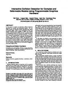
Figure 1: This simulation is generated using finite element solver on a mesh with about 9K triangles [Tang et al. 2011b]. Our novel continuous collision detection (CCD) algorithm takes about 1.1 second (on average) on a single CPU core to perform all intra-object and self-collision queries. It is about 5X faster than prior CCD algorithms for deformable models.

Abstract We present a fast algorithm for continuous collision detection between deformable models. Our approach performs no precomputation and can handle general triangulated models undergoing topological changes. We present a fast decomposition algorithm that represents the mesh boundary using hierarchical clusters and only needs to perform inter-cluster collision checks. The key idea is to compute such clusters quickly and merge them to generate a dynamic bounding volume hierarchy. The overall approach reduces the overhead of computing the hierarchy and also reduces the number of false positives. We highlight the the algorithm’s performance on many complex benchmarks generated from medical simulations and crash analysis. In practice, we observe 1.4 to 5 times speedup over prior CCD algorithms for deformable models in our benchmarks. CR Categories: I.3.3 [Computer Graphics]: Three-Dimensional Graphics and Realism—Physical Animation Keywords: Collision Detection, Topology Changes, Culling

1

Introduction

Continuous collision detection (CCD) is widely used in many applications, including physics-based simulation, computer-aided design, motion planning, etc. The main goal of CCD is to check for ∗ [email protected] † [email protected] ‡ [email protected] § [email protected]

collisions between the geometric primitives corresponding to two discrete time steps of a simulation. The simplest algorithms are based on linearly interpolating motion between the vertices of a mesh and computing the first time of contact along those trajectories. At the primitive level, the problem reduces to performing 15 elementary tests between the vertices, edges, and faces of the mesh using cubic polynomial root solvers. In this paper, we address the problem of efficient CCD between triangulated models undergoing topological changes. Such scenarios arise frequently in many applications: surgical simulation with cutting or tearing operations, crash analysis for CAD/CAM and material evaluation, fracture, explosions, etc. In these applications, the mesh connectivity may change or a large object may break into subobjects (or vice-versa). Our goal is to develop appropriate acceleration techniques or data structures to perform interactive continuous collision detection between triangulated models. Many techniques have been proposed in the literature for fast CCD queries. Most prior algorithms reduce the number of elementary tests between the primitives in one of three ways: by using some kind of acceleration data structures; by using the geometric properties of the mesh; or by using bounds on the motion of the objects or the primitives.. At a broad level, prior methods can be classified into high-level or low-level culling techniques. The highlevel techniques use bounding volume hierarchies, cluster decomposition, bounds on the normals, or bounds on the deformation to cull away non-overlapping primitives. The low-level techniques use simple filters or use connectivity information to reduce the number of elementary tests. Most of these methods perform some precomputation or exploit the connectivity information about the mesh; they work well in many applications (such as cloth simulation), but are less successful in representing objects that change topologically. Topological changes can result in new (sub)objects in the scene or can change the object connectivity. As a result, we need improved CCD algorithms that are applicable to all topology changing models and simulations. Main Results We present a general algorithm for CCD computations between triangulated models. Our approach is general and is used to check for inter-object and intra-object collisions. Our

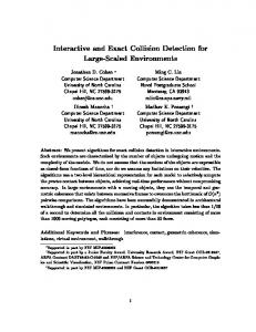
Figure 2: Sequence of simulation steps for the Car Crash benchmark with about 1.1-1.2 million triangles [Tang et al. 2011b]. We can reliably compute all collisions in about 15 seconds on a single core.

method uses a novel dynamic clustering scheme, which quickly decomposes the boundary of the objects into non self-colliding clusters. As compared to prior methods, our approach offers the following benefits: • The dynamic clustering strategy is general, efficient and involves no precomputation. • The merging algorithm results in tighter-fitting BVH, which reduces the number of elementary tests. • The cluster hierarchy is used to dynamically compute the BVH using a lazy approach, which reduces the runtime overhead of computing the BVH. We have implemented our algorithm, and we evaluate its performance on many complex benchmarks arising out of scenarios from crash analysis, medical simulation, and explosions. We have also compared with prior CCD algorithms based on BVHs and observe 1.4 − 5 times speedup in our benchmarks. The rest of the paper is organized as follows. We survey prior work on CCD in Section 2. We introduce the notation and give an overview of our approach in Section 3. We present our dynamic clustering algorithm in Section 4 and highlight its performance on various benchmarks in Section 5.

2

Prior Work

CCD has been well studied in the literature, and a number of techniques have been proposed to improve its efficiency and reliability. In this section, we give a brief overview of different methods. Bounding Volume Hierarchies (BVH) BVHs are widely used to speed up collision queries. Commonly used hierarchies are those based on simple bounding volumes such as axis aligned bounding boxes (AABBs) [van den Bergen 1998] and spheres [Hubbard 1995; Liang and Jur 2014]. Other algorithms that use tighter-fitting geometries include oriented bounding boxes (OBBs) [Gottschalk et al. 1996], discrete oriented polytopes (k-DOPs) [Klosowski et al. 1998], or their hybrid combination [Sanna and Milani 2004]. When working with deformable objects, these hierarchies need to be updated frequently in order to account for shape changes. There are various methods to update the BVH, including linear time refitting [Larsson and Akenine-Möller 2006], selective restructuring [Otaduy et al. 2007; Yoon et al. 2007] and kinetic data structures [Zachmann and Weller 2006]. Many techniques have also been proposed for handling self-collisions based on bound on normals [Provot 1997; Volino and Thalmann 1994; Tang et al. 2009; Heo et al. 2010], chromatic mesh decomposition [Govindaraju et al. 2005], or star-shaped decomposition [Schvartzman et al. 2010] or conservative advancement [Tang et al. 2010; Kim et al. 2014]. Bounds Computation Many techniques handle deforming objects by computing some bounds related to the deformation and

using them for self-collision culling. These types include subspace culling for reduced deformation [Barbiˇc and James 2010] and energy-based certificates for arbitrary deformation [Zheng and James 2012]. However, these techniques, which include an expensive precomputation step, may therefore not work well on models undergoing topological changes. Recently, [Wong et al. 2013; Wong et al. 2014] proposed a technique that accelerates continuous collision detection by performing radial view-based culling based on the skeleton structure. However, the skeleton needs to be precomputed and the overhead for models undergoing topology changes can be high. Decomposition Methods The many techniques to accelerate collision detection based on decomposition methods all, broadly speaking, decompose the boundary into clusters using some criteria and use the clusters to accelerate computation. These clusters have been used to compute tight-fitting bounding volume hierarchies from the bottom up [Tan et al. 1999] or used directly for collision detection [Wong et al. 2013; Wong et al. 2014; Ehmann and Lin 2001; Schvartzman et al. 2010; Wong and Baciu 2014]. However, all these techniques either perform some precomputation or assume fixed-mesh connectivity during the decomposition step. Reducing Elementary Tests Many techniques have been proposed to reduce the number of elementary tests between the triangle primitives [Govindaraju et al. 2005; Wong and Baciu 2005; Hutter and Fuhrmann 2007]. These include representative triangles [Curtis et al. 2008] and orphan sets [Tang et al. 2009], both of which reduce the number of duplicate elementary tests during collision checking. These algorithms, which exploit the connectivity information of a mesh, involve recomputation when the topology or connectivity information changes. Topological Changes Most general algorithms for topologychanging models involve recomputing the BVH for the entire scene, then performing continuous collision queries by traversing the BVH [Tang et al. 2011a]. But the BVH recomputation can have a high overhead. Many specialized collision-detection algorithms have been proposed: for CCD between volumetric meshes [Tang et al. 2011b], for objects undergoing fracture [Heo et al. 2010; Glondu et al. 2012] and for finite-element simulation of cuts [Wu et al. 2013]. Our approach is quite different from these specialized recent methods, and is applicable to all types of simulations. GPU-based Many fast techniques, proposed for collision detection between deformable models, exploit the parallel capabilities of many-core GPUs [Gress et al. 2006; Lauterbach et al. 2009; Pabst et al. 2010; Lauterbach et al. 2010; Tang et al. 2011a]. Many of these algorithms have also been used for interactive continuous collision detection on models undergoing topological changes. Our approach is orthogonal to the speedups obtained by GPU parallelization and can be accelerated using similar parallel methods. Reliable Collision Queries The underlying methods for primitive overlap tests during collision query are prone to error because of the calculations involved; since the elementary tests between linearly-

Triangle Mesh

Dynamic Clustering Leaf Cluster

Query Results

Intermediate Cluster

Elementary Tests

BVH Tree Construction Lazy BVH Traversal

Figure 3: High level description of our approach highlighting various stages of the algorithm.

interpolating triangles reduce to finding roots of a cubic polynomial, and the floating-point solvers used to compute these roots are prone to errors, this can affect the reliability of collision queries. Our algorithm can use any of the many recently-proposed techniques for avoiding these errors [Brochu et al. 2012; Wang 2014; Tang et al. 2014], since the choice of the algorithm used to perform elementary tests is orthogonal to our approach.

3

Background and Overview

In this section, we give an overview of our algorithm. We present the problem definition and introduce the notation and terminology used in the rest of the paper. We give an overview of our approach and present the decomposition scheme.

3.1

Problem Definition

We assume that we are given a scene composed of one or more objects. Each object is represented as a triangle mesh and may correspond to an open or closed object. We assume that it is possible to perform a local inside/outside classification with respect to each triangle in the mesh and that each triangle normal is pointing outward. During the simulation, the objects may undergo motion or deformations, which can change their topology or generate new vertices and triangles; while the connectivity information may change, we assume that the new set of objects are still represented as triangular meshes with local inside/outside classification. Given two discrete time instances in a simulation, we assume that the vertices of the objects move at a constant velocity during that time interval. If new vertices are generated due to topology changes, the CCD problem is then posed as a problem of defining appropriate mapping between the two discrete instances. Our goal is to check whether there is any collision, including self-collisions, during that time interval, which we represent as t ∈ [0, 1]. For two triangles, this computation reduces to performing 15 elementary tests corresponding to vertex-face (VF) and edge-edge (EE) pairs. Given a CCD query, we assume that there are no collisions among the primitives at t = 0. This assumption can be easily checked by using a discrete collision detection algorithm.

3.2

Notation

In this paper, we will use the following notation. The symbol M will represent a triangle mesh of an object, τ represents a single triangle and T represents a set of connected triangles. We use the symbol ν to represent a vertex. Our algorithm decomposes the boundary of each mesh into clusters,

Figure 4: We highlight the cluster hierarchy that is generated for each object in the scene. Initially we generate the leaf clusters (LC) then merge those to generate intermediate-level clusters. (IC).

which are represented as Ci , i = 0, 1, 2..., n, for n+1 total number of clusters. We associate an observation point with each cluster. These observation points are represented as Oi . Tk represents the set of connected triangles belonging to a single cluster and Vk is the set of vertices for a single cluster. We represent these clusters using a hierarchy: LC represents the lowest level or leaf cluster of the hierarchy and IC represents an intermediate cluster in the hierarchy.

3.3

Overview

The simplest general algorithms for CCD between models undergoing topological changes are based on computing a BVH of all the objects in the scene. The leaf nodes of the BVH correspond to the triangle primitives and the intermediate nodes correspond to the bounding volumes (e.g. k-DOPs). Prior CCD algorithms traverse the BVH and perform the CCD queries between the overlapping primitives. Since the connectivity information in the mesh changes when the topology changes, prior techniques that used connectivity information to reduce the number of elementary tests are not directly applicable. As a result, prior algorithms would need to recompute the BVH for the entire scene using top-down or bottom-up manner, which can become expensive for complex scenes with a lot of objects. In order to speed this CCD computation, we decompose the object boundaries into clusters. The overall pipeline of our method is shown in Figure 3. Our approach uses a new dynamic clustering scheme. It generates the clusters in an incremental manner by traversing the triangles on the mesh boundary, and makes no assumptions about topology or connectivity changes. We denote these clusters as LC, which correspond to the lowest level of clusters (or leaf clusters) in the final cluster hierarchy (see Figure 4). Moreover, we ensure that each cluster has no self-collisions among its triangle primitives. As a result, CCD reduces to querying only for inter-cluster collisions. There are two key issues that arise in terms of computing such leaf clusters. The first issue is that, while we want to decompose the boundary into as few clusters as possible, the problem of computing that minimal number of clusters based on some standard criterion (e.g. convexity) tends to be NP-hard [Chazelle et al. 1997]. To overcome this issue, we compute these clusters using a greedy strategy. The second issue is that the clusters must be computed efficiently during each frame, as the object’s topology may change from frame to frame. Our next step is to merge these leaf clusters to generate the intermediate clusters (ICs); each of these intermediate clusters is also guaranteed to have no self-collisions. Our algorithm merges various neighboring LCs, while the merged cluster preserve the no selfcollision property, see Figure 4. Now that we have computed the IC and LC, we use them to generate a BVH. The upper level nodes of the BVHs are obtained by combining different ICs in a bottom-up manner. We traverse the tree in a top-down manner and check the bounding volume of each

IC and LC for collisions. If we need to check two LCs for further collision, we compute the corresponding BVHs in a lazy manner (see Figure 5). Based on this formulation, we can limit our BVH computation to those of only a few LCs, rather than computing BVHs for all the LC i or all the triangles in the scene. This overall approach reduces the time spent in BVH computation during each frame, and our use of a cluster hierarchy gives a much tighter-fitting BVH.

vertices (i = 0, 1, 2) of the same triangle; we can therefore use any of those vertices to define this function. We define LC as a cluster of triangles with respect to a single observation point O at a given time t satisfying: φ(τ, O, t) ≥ 0.

(2)

The computation of the observation point O is a key issue in terms of computing a cluster LC, since it is used to define the function φ and its location will affect the size and location of the resulting cluster. We start with a triangle τ on the mesh that remains outside LC. The observation point is set at the centroid of the triangle τ : O = (ν0 + ν1 + ν2 )/3,

(3)

where ν0 , ν1 , ν2 are the three vertices of the triangle. Next, we compute concentric loops (or rings) of triangles in order to ensure that they are facing away from the observation point. This ensures that the mesh formed is not self-intersecting.

Figure 5: The BVH is computed from the leaf and intermediate clusters. We use a binary tree and combine the nodes using appropriate bounding volumes (e.g. k-DOPs). BV H(LC i ) is constructed only for potentially colliding leaf clusters LC i in a lazy manner (it is computed only when needed to check for collisions).

4

Dynamic Clustering

In this section, we introduce our dynamic clustering algorithm. Our approach works in three steps. First, we compute the leaf cluster LCs in a greedy manner. Next, we merge these leaf clusters in order to compute the intermediate clusters (IC). Finally, we compute the dynamic BVH based on the ICs in a lazy manner and traverse the tree to perform collision queries.

4.1

Leaf Clusters

In this section, we present our approach for computing the leaf clusters. Note that we need to ensure that each LC has no selfcollisions, and that we want to decompose the boundary of a mesh into as few LCs as possible. Our formulation uses the notion of an observation point, introduced by [Wong et al. 2013; Wong et al. 2014], to compute these clusters using an adaptive scheme. Our method computes the relative orientation of a normal of a triangle with respect to the vector joining any vertex of the triangle and an observation point. We assume that the front face of each triangle is outside facing. We exploit the fact that all the triangles that enclose a connected area of the mesh and have their backfaces visible from the observation point cannot intersect each other. We define the characteristic time dependent function as φ(τ, O, t) = n(t) · (ν0 (t) − O(t)),

(1)

for a triangle τ , with respect to an observation point O at time t. Here n(t) is the triangle normal and νi (t) is the position of the vertex at time t. Note that the sign of φ does not change for different

Figure 6: Incremental computation of a leaf cluster. Initially, we choose an unassigned triangle T0 (shown in red). We then collect the triangles connected (shown in blue) to T0 and name the collection T1 , lastly T2 (shown in green) is constructed by collecting the triangles incident to T1 but not belonging to it. In general, this ensures that the triangles belonging to Ti form a loop (or ring) around the triangles belonging to Ti−1 .

We first set T0 = {τ } and proceed in an incremental manner expanding collections of triangle loops and forming a leaf cluster LC = T0 ∪ T1 ∪ . . . (see Figure 6). This incremental approach assume that T0 does not collide with any triangle in T1 , T 2 , . . . . This is a reasonable assumption since T0 contains only one triangle and all triangles in T1 are adjacent to T0 . In order to compute Ti from Ti−1 , we consider all the triangles that are incident to the vertices in Vi−1 and do not belong to Ti−1 . Figure 6 illustrates how three such triangle sets are computed from a single initial triangle. If all of triangles in Ti satisfy φ(τ, O, t) ≥ 0, then we add all triangles of Ti to LC. In this case, the new leaf cluster LC corresponds to all the triangles that belong to the union of T0 , T1 . . . , Ti−1 . If we encounter a triangle such that φ(τ, O, t) < 0, we then terminate this iterative process and define a new set of vertices V i consisting of the vertices of Ti triangles excluding vertices in other loops as: V = {ν | ν ∈ Vi , ν ∈ / Vj , j = 0, ..., i − 1}.

(4)

Our classification criteria is conservative and ensures that all the triangles belonging to the leaf cluster LC do not self-intersect. This process is repeated until the triangles on the boundaries of all the objects are assigned to one of the leaf clusters. Depending on the choice of the initial triangle (i.e. τ in T0 ), we can get a high number of leaf clusters.

Note that we do not compute the BVs for the two clusters LC i−1 and LC i explicitly, since they are neighbors their BVs likely overlap and would be forced to be splitted into smaller BVs. Rather we check for overlaps by using properties of these clusters in terms of various loops and check if two specific bounding volumes, Bi and 0 Bi−1 overlap. This results in a considerable performance improvement.

Figure 7: This figure shows the 2D profile of two adjacent clusters LC i−1 and LC i . The center figure shows the the overlapping BVs. In the right figure we use Algorithm 1 to remove the last triangle loop of LC i−1 and merged the remained triangles into LC i .

4.2

Intermediate Clusters

The algorithm for leaf cluster computation decomposes the boundary into a large number of leaf node clusters. In this section, we describe our approach to merge leaf clusters to generate the intermediate clusters. We combine neighboring or adjacent IC (i.e. the ones sharing common edges) and use the observation points associated with those adjacent clusters to compute a new observation point for the merged cluster. Consider two adjacent clusters LC i−1 and LC i and suppose that their initial observation points are Oi−1 and Oi , respectively. Our goal is to decide whether or not to merge these clusters. The intermediate clusters are built from sequences of leaf clusters. First, we calculate the observation point Oi for each leaf cluster as follows: P j νj Oi = , νj ∈ V i . (5)

V i In other words, we take the average location

among the vertices in V i , as defined by Equation (4). Here V i represents the cardinality of V i . Next, we determine if LC i and LC i−1 have any overlapping or colliding triangles. Initially, Oi is treated as a potential observation point for this new, merged cluster. We use the criteria given by Equation 2 to check if T i−1 and T i are collision free, i.e. no additional collision exist besides overlapping boundary edges, see Figure 7. We know that the triangles in T i satisfy this criterion, as they are backfacing w.r.t. Oi . So we are left to check whether all the triangles in T i−1 also satisfy the criterion in Equation (2) with respect to the observation point Oi . If the two triangle sets T i−1 and T i are indeed collision free, we then com0 pute the boundary volumes Bi and Bi−1 of LC i and LC i−1 −T i−1 , 0 respectively. Finally, if Bi and Bi−1 do not overlap, then LC i and LC i−1 do not have any colliding triangles, thus they can be merged into an intermediate cluster IC. Lemma 1. Given two adjacent leaf clusters: LC i−1 and LC i , assume that they satisfy the following conditions: φ(τ, Oi , t) ≥ 0, τ ∈ T i−1 ∪ T i .

(6)

0

Consider the triangle set LC i−1 = LC i−1 − T i−1 ⊂ LC i−1 . If 0 LC i−1 and LC i are not colliding, then LC i−1 and LC i are also collision free, and can be merged. Proof. If all triangles in T i−1 satisfy Equation (6), then T i−1 and LC i are collision free. If LC i has no overlap or collision with 0 0 LC i−1 , then LC i and LC i−1 are also collision free. As a result, 0 there is no collision between LC i and LC i−1 = LC i−1 ∪T i−1 .

Algorithm 1 Given two clusters and an observation point, check whether the clusters are collision free. 1: C OLLIDING C LUSTERS(LC i , LC i−1 , Oi ) 2: for τ ∈ T i ∪ T i−1 do 3: if φ(τ, Oi , t) < 0 then 4: return FALSE. 0 5: if Bi ∩ Bi−1 6= N U LL then 6: return FALSE. 7: return TRUE.

We process all pairs of leaf clusters and add them to an intermediate cluster in the following manner. Suppose we have a set of merged leaf clusters LC i , i = 0, 1, 2..., n − 1. We label the intermediate cluster as IC and their corresponding bounding volumes as B0 , B1 , . . . , Bn−1 and its union as BIC = B0 ∪ B1 , . . . , Bn−1 . In order to add an additional neighboring cluster LC n to IC, we first check if these two clusters, LC n and LC n−1 , can indeed be merged using Algorithm 1. If they can be merged, we then check if the combined BVs B0 ∪ B1 , . . . , Bn−2 do not overlap with Bn . If there is no overlap, then we add LC n to IC, otherwise LC n will will be used to defined another intermediate cluster. This process is repeated until all leaf clusters have been assigned to one intermediate cluster. Algorithm 2 gives a description of the algorithm.

Algorithm 2 Verify whether it is possible to merge a leaf cluster LC i to IC. 1: M ERGE C LUSTER(LC i , IC, Oi ) 2: if C OLLIDING C LUSTERS(LC i , LC i−1 , Oi ) == FALSE then 3: return FALSE. 4: if {BIC − Bi−1 } ∩ Bi 6= N U LL then 5: return FALSE. // BVs overlap 6: return TRUE.

4.3

BVH Tree Computation

Given the cluster hierarchy, the last step of our algorithm involves the computation of the BVH. Note that we have multiple intermediate clusters IC (see Figure 5) and each these clusters has no selfcollisions. The CCD problem then reduces to performing collision checks between various clusters (i.e. inter-cluster collisions). Since we can get a high number of clusters (say N ), we want to avoid performing O(N 2 ) cluster-cluster collision checks. We use a BVH to accelerate this computation. The BVH computation is performed in two steps. We first merge all the intermediate clusters and generate a binary tree in a bottom-up manner. We start with the topmost nodes corresponding to the IC. We compute the BVs in terms of k-DOPs. The leaf nodes of this tree correspond to LCs, as shown in Figure 4. However, we do not precompute the BVHs for all of the leaf clusters. Rather, we compute the only the BVHs that correspond to all the triangles within a particular LC in a lazy manner, and perform collision checking. For example, in Figure 5, we compute the BVH for only two of the leaf clusters. This lazy approach of computing a BVH results in

of triangles per cluster can vary; since the bunny/dragon benchmark, for example, results in a large number of sub-objects, it has fewer triangles per cluster than the other benchmarks, which have far more triangles per cluster.

Figure 8: We test our method on different deformable models and topology changing scenarios [Tang et al. 2011a]. We compute the BVHs using k-DOP as the underlying bounding volume and the CCD query computes the first time of contact, including selfcollisions.

considerable runtime savings and overhead of BVH computation. For instance, if there are no collisions, or only a few isolated collisions, we compute only the BVH corresponding to the few LCs that displayed collisions. Each node of the BVH computed in a lazy manner corresponds to a k-DOP. Given the BVH, we then perform overlap tests between the nodes. For overlapping nodes at the leaf level, we perform the 15 elementary tests between the triangles to check for possible collisions.

5

In the benchmarks where a number of new sub-objects are generated during the simulation, we need to perform dynamic clustering on each sub-object, which increases the total time spent in the dynamic clustering stage for these benchmarks (e.g. for lion, bunny/dragon, and car-crashing benchmarks). We use k-DOPs as the underlying BVs of the BVH. The time spent in BVH computation can be divided into two parts: first, the time spent building the BVH in a bottom-up manner, starting from the leaf clusters, computing bounding volumes (BV) around the intermediate clusters (IC), and computing the trees, looking for potentially colliding pairs of clusters. Second, most of the BVH computation time is spent traversing the BVH and performing elementary tests between the vertices, edges, and faces of the mesh. This second stage of the algorithm dominates the computation. As we notice in Table 1, columns BVH and Elementary Test (Elem. Test), our dynamic clustering algorithm and the lazy strategy results in fewer BV overlap tests as well as elementary tests. This is because our clustering scheme results in tighter-fitting BVs and the lazy strategy implies that we have to perform fewer BV computations. These efficiencies explain the overall improvements in performance displayed by our algorithm.

Implementation and Results 5.2

In this section, we describe our implementation and compare its performance with prior techniques. Our algorithm is implemented in C++ on a Intel Core i7 CPU running at 3.30GHz with 16GB of RAM on Window 7 (64-bits) personal computer. All the performance and timing results were generated using a single core. We have used our algorithm on different benchmarks described below: • Nidus: This benchmark models the nidus of an Arteriovenous Malformation (AVM) segmented from an MRA dataset, and is used for surgical simulation. We have two versions of the models: one represents large deformation, the other cutting operations.

We have compared the performance of our algorithm with that of prior algorithms available as part of the Self-CCD package.1 SelfCCD computes a new BVH for the model at each frame [Tang et al. 2009] and traverses the hierarchies to cull away non-overlapping primitives. It also uses non-penetration filters to accelerate the elementary tests. Compared to Self-CCD, we observe speedups of 1.4-5 times with our approach. This is mainly due to fewer BV overlap tests and elementary tests. As the number of objects or subobjects in the scene increases, the overhead of dynamic clustering also increases, and we observe lower speedups.

• Airbag: This is a model of an airbag simulated using FEM. It has self-collisions and collisions with the wheel.

Nidus Airbag Lion Bunny Car Crash

• Lion: The complex model of a lion explodes and breaks into various pieces that collide with each other. • Bunny/Dragon: This is a dynamic simulation of a bunny breaking a dragon into small pieces • Car Crash: The FEM model of a Ford Explorer with 1.1 million triangles crashes against a wall. This results in large topology changes and self-collisions.

5.1

Comparison

Triangles

LC

IC

Ratio

32,798 9,076 1.6M 0.25M-0.27M 1.1M-1.2M

581 145 14376 4,315 5331

116 32 2,556 3321 843

282 283 626 75 1,049

Table 2: Model Complexity and Dynamic Clustering: We highlight the geometric complexity of these models. The number of leaf clusters (LC), intermediate clusters (IC) and the average number of triangles per cluster (shown as Ratio).

Analysis

Table 1 shows how much time is spent in each of the algorithm; the time displayed includes the dynamic generation of clusters, the BVH computation, and all collision queries performed using tree traversal. As the table indicates, the time spent in the dynamic clustering phase is relatively small compared to the time required for the other two phases. This is because the cluster-computation algorithm performs orientation tests based on the characteristic function φ (Eq. 1), which involves a few arithmetic operations and a dot product. Similarly, Table 2 indicates that the overhead of the merging algorithm used to compute the intermediate clusters is also low; our merging algorithm can reduce the number of clusters considerably (e.g. up to 5 times). As the tables show, the average number

6

Limitations and Conclusions

In this paper, we have presented an algorithm for CCD queries between models undergoing topological changes. Our approach is general and applicable to all triangulated models. We use a decomposition scheme based on dynamic clustering. The algorithm generates leaf-level clusters and merges them to generate intermediate clusters. The BVH is computed in a lazy manner from the cluster hierarchy and is used to perform CCD queries. We have highlighted our algorithm’s performance on different benchmarks, 1 http://gamma.cs.unc.edu/SELFCD/

Figure 9: Sequence of simulation steps for the AVM Nidus benchmark with about 33K triangles. Large deformation are computed using a linear finite element solver and the average CCD query takes about 56ms.. Self-CCD Tree Traversal + Elem. Tests 142ms Nidus 5,325ms Airbag 14,673ms Lion Bunny/Dragon 45,145ms 21,732ms Car Crash

Our Method

BVH Construction

Total Query time

BVH Tests

Elem. Tests

4ms 3ms 160ms 26ms 216ms

146ms 5,328ms 14,833ms 45,771ms 21,948ms

676,512 953,649 79,693,697 6,317,304 87,273,186

146 5328 14,833 45,171 21,948

Tree Traversal + Elem. Tests 32ms 1,098ms 5,097ms 32,307ms 14,041ms

BVH Construction

Dynamic Clustering

Total Query time

BVH Tests

Elem. Tests

4ms 2ms 116ms 23ms 256ms

17ms 16ms 361ms 442ms 1,198ms

53ms 1,116ms 5,574ms 32,772ms 15,495ms

51,332 53, 989 15,322,834 1,316,105 23,335,076

52 1,168 5,584 32,948 14,232

Table 1: Comparison: We compare the performance of our approach with Self-CCD algorithm and package. We report average query times for: “BVH Construction” is the time spent in tree construction; “Dynamic Clustering” is the time spent in dynamic clustering; "Elem. Tests" is the time spent in performing EE and VF elementary tests; "Tree Traversal" is the time spent in traversing the tree and bounding volume overlap tests; “Total Query Time” is the total time for CCD query on these complex models with topology changes. We also report the average number of bounding volume (BV) overlap tests and elementary tests performed during each frame. Due to clustering and lazy BVH construction, our algorithm results in fewer BV tests and elementary tests.

and we observe 1.4 to 5 times speedup over prior algorithms and implementations. Our approach has a few limitations. The dynamic clustering scheme has an overhead that increases with the number of objects or subobjects within the scene. As a result, we observe less benefit on simulations that that generate many small objects (e.g. lion or bunnydragon benchmarks). Our criteria for generating leaf clusters works best when the object does not have many sharp edges or highly varying curvature. We also assume that the underlying simulation generates models with consistent normals and that it is possible to locally classify them into inside-outside regions; this may not be true for all objects. There are many avenues for future work. We would like to parallelize our dynamic clustering algorithm on multi-core processors or GPUs. Furthermore, we would like to integrate our CCD algorithm into FEM, fracture or medical simulation systems and evaluate its performance. Finally, we would like to design improved dynamic simulation algorithms that can exploit the capabilities of the CCD algorithm in terms of adaptive time-stepping and collision response.

Acknowledgment This research is supported in part by ARO Contract W911NF-141-0437, NSF grant 1305286 and the Office Of The Director, National Institutes Of Health under Award Number R44OD018334. The content is solely the responsibility of the authors and does not necessarily represent the official views of the National Institutes of Health. We are also grateful to Min Tang for providing the benchmarks and useful discussions.

References BARBI Cˇ , J., AND JAMES , D. L. 2010. Subspace self-collision culling. ACM Trans. on Graphics (SIGGRAPH 2010) 29, 4,

81:1–81:9. B ROCHU , T., E DWARDS , E., AND B RIDSON , R. 2012. Efficient geometrically exact continuous collision detection. ACM Trans. Graph. 31, 4 (July), 96:1–96:7. C HAZELLE , B., D OBKIN , D. P., S HOURABOURA , N., AND TAL , A. 1997. Strategies for polyhedral surface decomposition: an experimental study. Comput. Geom. 7, 327–342. C URTIS , S., TAMSTORF, R., AND M ANOCHA , D. 2008. Fast collision detection for deformable models using representativetriangles. In Proceedings of the 2008 Symposium on Interactive 3D Graphics and Games, ACM, New York, NY, USA, I3D ’08, 61–69. E HMANN , S. A., AND L IN , M. C. 2001. Accurate and fast proximity queries between polyhedra using convex surface decomposition. In Computer Graphics Forum, 500–510. G LONDU , L., S CHVARTZMAN , S. C., M ARCHAL , M., D U MONT, G., AND OTADUY, M. A. 2012. Efficient collision detection for brittle fracture. In Proceedings of the ACM SIGGRAPH/Eurographics Symposium on Computer Animation, SCA ’12, 285–294. G OTTSCHALK , S., L IN , M. C., AND M ANOCHA , D. 1996. Obbtree: A hierarchical structure for rapid interference detection. In Proceedings of ACM SIGGRAPH, 171–180. G OVINDARAJU , N. K., K NOTT, D., JAIN , N., K ABUL , I., TAM STORF, R., G AYLE , R., L IN , M. C., AND M ANOCHA , D. 2005. Interactive collision detection between deformable models using chromatic decomposition. In ACM Transactions on Graphics (TOG), vol. 24, 991–999. G RESS , A., G UTHE , M., AND K LEIN , R. 2006. Gpu-based collision detection for deformable parameterized surfaces. Computer Graphics Forum 25, 3, 497–506.

H EO , J.-P., S EONG , J.-K., K IM , D., OTADUY, M. A., H ONG , J.-M., TANG , M., AND YOON , S.-E. 2010. Fastcd: Fracturingaware stable collision detection. In Proceedings of the 2010 ACM SIGGRAPH/Eurographics Symposium on Computer Animation, 149–158. H UBBARD , P. M. 1995. Collision detection for interactive graphics applications. IEEE Transactions on Visualization and Computer Graphics 1, 3 (Sept.), 218–230. H UTTER , M., AND F UHRMANN , A. 2007. Optimized continuous collision detection for deformable triangle meshes. Journal of WSCG 15, 1-3, 25–32. K IM , Y. J., M ANOCHA , D., AND TANG , M. 2014. Hierarchical and controlled advancement for continuous collision detection of rigid and articulated models. IEEE Transactions on Visualization and Computer Graphics 20, 5, 755–766. K LOSOWSKI , J. T., H ELD , M., M ITCHELL , J. S. B., S OWIZRAL , H., AND Z IKAN , K. 1998. Efficient collision detection using bounding volume hierarchies of k-dops. IEEE Transactions on Visualization and Computer Graphics 4, 1 (Jan.), 21–36. L ARSSON , T., AND A KENINE -M ÖLLER , T. 2006. A dynamic bounding volume hierarchy for generalized collision detection. Computers & Graphics 30, 3, 450–459. L AUTERBACH , C., G ARLAND , M., S ENGUPTA , S., L UEBKE , D., AND M ANOCHA , D. 2009. Fast bvh construction on gpus. In IN PROC EUROGRAPHICS 09.

formable models using connectivity-based culling. IEEE Transactions on Visualization and Computer Graphics 15, 544–557. TANG , M., M ANOCHA , D., AND T ONG , R. 2010. Mccd: Multicore collision detection between deformable models using frontbased decomposition. Graphical Models 72, 2, 7–23. TANG , M., M ANOCHA , D., L IN , J., AND T ONG , R. 2011. Collision-streams: Fast gpu-based collision detection for deformable models. In Symposium on Interactive 3D Graphics and Games, ACM, New York, NY, USA, I3D ’11, 63–70. TANG , M., M ANOCHA , D., YOON , S.-E., D U , P., H EO , J.-P., AND T ONG , R.-F. 2011. Volccd: Fast continuous collision culling between deforming volume meshes. ACM Trans. Graph. 30, 5 (Oct.), 111:1–111:15. TANG , M., T ONG , R., WANG , Z., AND M ANOCHA , D. 2014. Fast and exact continuous collision detection with bernstein sign classification. ACM Trans. Graph. 33, 6 (Nov.), 186:1–186:8. B ERGEN , G. 1998. Efficient collision detection of complex deformable models using aabb trees. J. Graph. Tools 2, 4 (Jan.), 1–13.

VAN DEN

VOLINO , P., AND T HALMANN , N. M. 1994. Efficient selfcollision detection on smoothly discretized surface animations using geometrical shape regularity. In Computer Graphics Forum, vol. 13, Wiley Online Library, 155–166. WANG , H. 2014. Defending continuous collision detection against errors. ACM Transactions on Graphics (TOG) 33, 4, 122.

L AUTERBACH , C., M O , Q., AND M ANOCHA , D. 2010. gproximity: Hierarchical gpu-based operations for collision and distance queries. Computer Graphics Forum 29, 2, 419–428.

W ONG , W. S.-K., AND BACIU , G. 2005. Dynamic interaction between deformable surfaces and nonsmooth objects. IEEE Transactions on Visualization and Computer Graphics 11, 3, 329–340.

L IANG , H., AND J UR , VAN , D. B. 2014. Efficient exact collision checking of 3d rigid body motions using linear transformations and distance computations in workspace. In Proceedings of the IEEE International Conference on Robotics and Automation(ICRA).

W ONG , S.-K., AND BACIU , G. 2014. Continuous collision detection for deformable objects using permissible clusters. The Visual Computer, 1–13.

OTADUY, M., C HASSOT, O., S TEINEMANN , D., AND G ROSS , M. 2007. Balanced Hierarchies for Collision Detection between Fracturing Objects. In Virtual Reality Conference, 2007. VR ’07. IEEE, IEEE, 83–90. PABST, S., KOCH , A., AND S TRASSER , W. 2010. Fast and scalable cpu/gpu collision detection for rigid and deformable surfaces. In Computer Graphics Forum, vol. 29, 1605–1612. P ROVOT, X. 1997. Collision and self-collision handling in cloth model dedicated to design garments. Computer Animation and Simulation ’97, Eurographics 1997, 177–189.

W ONG , S.-K., L IN , W.-C., H UNG , C.-H., H UANG , Y.-J., AND L II , S.-Y. 2013. Radial view based culling for continuous selfcollision detection of skeletal models. ACM Trans. Graph. 32, 4 (July), 114:1–114:10. W ONG , S.-K., L IN , W.-C., WANG , Y.-S., H UNG , C.-H., AND H UANG , Y.-J. 2014. Dynamic radial view based culling for continuous self-collision detection. In Proceedings of the 18th Meeting of the ACM SIGGRAPH Symposium on Interactive 3D Graphics and Games, 39–46. W U , J., D ICK , C., AND W ESTERMANN , R. 2013. Efficient collision detection for composite finite element simulation of cuts in deformable bodies. The Visual Computer 29, 6-8, 739–749.

S ANNA , A., AND M ILANI , M. 2004. Cdfast: an algorithm combining different bounding volume strategies for real time collision detection. SCI Proceedings 2, 144–149.

YOON , S.-E., C URTIS , S., AND M ANOCHA , D. 2007. Ray tracing dynamic scenes using selective restructuring. In Proceedings of the 18th Eurographics Conference on Rendering Techniques, 73–84.

S CHVARTZMAN , S. C., P EREZ , A. G., AND OTADUY, M. A. 2010. Star-contours for efficient hierarchical self-collision detection. ACM Trans. on Graphics (Proc. of ACM SIGGRAPH) 29, 3.

Z ACHMANN , G., AND W ELLER , R. 2006. Kinetic bounding volume hierarchies for deformable objects. In Proceedings of the 2006 ACM International Conference on Virtual Reality Continuum and Its Applications, 189–196.

TAN , T.-S., C HONG , K.-F., AND L OW, K.-L. 1999. Computing bounding volume hierarchies using model simplification. In Proceedings of the 1999 symposium on Interactive 3D graphics, ACM, 63–69.

Z HENG , C., AND JAMES , D. L. 2012. Energy-based self-collision culling for arbitrary mesh deformations. ACM Transactions on Graphics (Proceedings of SIGGRAPH 2012) 31, 4 (Aug.).

TANG , M., C URTIS , S., YOON , S.-E., AND M ANOCHA , D. 2009. Iccd: Interactive continuous collision detection between de-