Latent Variables in a Travel Mode Choice Model - Diva Portal

Working Paper 2005:5 Department of Economics

Latent Variables in a Travel Mode Choice Model: Attitudinal and Behavioural Indicator Variables Maria Vredin Johansson, Tobias Heldt and Per Johansson

Department of Economics Uppsala University P.O. Box 513 SE-751 20 Uppsala Sweden Fax: +46 18 471 14 78

Working paper 2005:5 February 2005 ISSN 0284-2904

LATENT VARIABLES IN A TRAVEL MODE CHOICE MODEL: ATTITUDINAL AND BEHAVIOURAL INDICATOR VARIABLES MARIA VREDIN JOHANSSON, TOBIAS HELDT AND PER JOHANSSON

Papers in the Working Paper Series are published on internet in PDF formats. Download from http://www.nek.uu.se or from S-WoPEC http://swopec.hhs.se/uunewp/

Latent Variables in a Travel Mode Choice Model: Attitudinal and Behavioural Indicator Variables∗ Maria Vredin Johansson†, Tobias Heldt‡and Per Johansson§

Abstract In a travel mode choice context, we use survey data to construct and test the significance of five individual specific latent variables - environmental preferences, safety, comfort, convenience and flexibility postulated to be important for modal choice. Whereas the construction of the safety and environmental preference variables is based on behavioural indicator variables, the construction of the comfort, convenience and flexibility variables is based on attitudinal indicator variables. Our main findings are that the latent variables enriched discrete choice model outperforms the traditional discrete choice model and that the construct reliability of the “attitudinal” latent variables is higher than that of the “behavioural” latent variables. Important for the choice of travel mode are modal travel time and cost and the individual’s preferences for flexibility and comfort as well as her environmental preferences. Key words: Modal Choice, Latent Variable, Discrete Choice Model, Modal Safety JEL Classifications: C35, R41

∗ The authors thank seminar participants at the Department of Economics at Uppsala university and the Swedish National Road and Transport Research Institute in Borlänge for useful suggestions. Financial support for Maria Vredin Johansson from The Swedish National Road Administration and The Wallenberg Foundation is gratefully acknowledged. The paper is also published as VTI notat 6A-2004. The usual disclaimer applies. † Department of Economics, Uppsala university, P. O. Box 513, SE-751 20 Uppsala and Swedish National Road and Transport Research Institute, P. O. Box 760, 781 27 Borlänge, Sweden. Email: [email protected] ‡ Department of Economics, Uppsala university, P. O. Box 513, SE-751 20 Uppsala, Sweden and Department of Economics and Society, Dalarna university, SE-781 88 Borlänge, Sweden. Email: [email protected] § Department of Economics, Uppsala university and Institute for Labour Market Policy Evaluation, P. O. Box 513, SE-751 20 Uppsala, Sweden. Email: [email protected]

Latent Variables in a Travel Mode Choice Model...

1

1

Introduction

In designing a socially desirable and environmentally sustainable transport system in line with people’s preferences, transport planners must increase their understanding of the hierarchy of preferences that drive individuals’ choice of transport. Understanding modal choice is important since it affects how efficiently we can travel, how much urban space is devoted to transport functions as well as the range of alternatives available to the traveller (Ortúzar and Willumsen, 1999, ch. 6). In the empirical literature on travel mode choice, most choice models use modal attributes to explain choice. Individual specific variables are also often included to control for individual differences in preferences and unobservable modal attributes. This paper specifically addresses the problem of unobservable, or latent, preferences in modal choice models. The overriding purpose is to examine whether constructions of latent variables, mirroring the individual’s preferences, are able to provide insights into the individual’s decision making “black box” and, thus, to help to set priorities in governmental policy and decision making. In recent attempts to gain insight into the decision making process of the individual, traditional choice models have been enriched with constructions of latent variables (McFadden, 1986; Morikawa and Sasaki, 1998; Ben-Akiva et al., 1999; Pendleton and Shonkwiler, 2001; Morikawa et al., 2002; Ashok et al., 2002). For example, Morikawa and Sasaki (1998) and Morikawa et al. (2002) include modal comfort and convenience in their analyses of modal choice. In their applications, the latent variables are measured and modelled through attitudes (attitudinal indicator variables) towards the chosen and an alternative travel mode. In this paper, we model five latent variables and a maximum of three alternative travel modes. We use individual specific, not mode specific, latent variables to explain choice which means that we do not construct latent variables for nonchosen modes. Since the individual’s opinion of nonchosen modes could be influenced by the individual’s chosen mode, there is a risk of endogeneity when constructing latent variables for nonchosen modes. Through a survey in a commuter context, data are collected on the respondent’s modal choice and on the attitudinal and behavioural indicator variables that are used to construct environmental preferences and preferences for safety, flexibility, comfort and convenience.1 The construction of the safety and environmental preference variables is based on behavioural indicator variables and the construction of the comfort, convenience and flexibility variables is based on attitudinal indicator variables. Thus, we are able to compare the explanatory power of constructions based on either type of indicator variables. Whereas inclusion of preferences for comfort, 1

The questionnaire is available from the authors upon request.


2

convenience and flexibility needs little explanation, there are several reasons for our interest in safety and environmental preferences. Preferences for safety are interesting mainly because reduced casualties is a major benefit of road infrastructure projects. In the cost benefit analyses (CBA) of the Swedish National Road Administration (SNRA), the value of increased safety represents roughly a third of all monetized benefits from infrastructural projects (Naturvårdsverket, 2003). The value of statistical life presently applied is derived from a Swedish contingent valuation (CV) study (SIKA, 2002; Persson et al., 1998).2 Since CV studies can only uncover stated preferences, the resulting value can always be criticized for being hypothetical (e.g. Diamond and Hausman, 1995). Furthermore, several CV studies have revealed people’s difficulties in understanding and valuing risk changes (Hammitt and Graham, 1999; Smith and Desvousges, 1987; JonesLee et al., 1985). Thus, the value of statistical life from CV surveys may be questioned. Since our survey is based on revealed preferences, we hope to shed light on whether preferences for safety are important in a real mode choice situation. Proenvironmental preferences are of interest because there is an increased interest in incorporating environmental impacts in cost benefit analyses and the SNRA decision making. Because conversion to an environmentally sustainable transport system will, by necessity, affect peoples’ choice of transport we find it interesting to gain increased knowledge about the importance of environmental aspects in peoples’ choice of travel mode. Previous research has, however, shown little support for environmental criteria being of importance in travel mode choices (Daniels and Hensher, 2000; Vredin Johansson, 1999). We estimate the individual’s preferences in a latent variable model and include predictions of the latent variables in a discrete choice model for modal choice (multinomial probit with varying choice sets). On several accounts our “latent variables enriched” choice model outperforms a traditional choice model and provides insights into the importance of unobservable individual specific variables in modal choice. Whereas environmental preferences, comfort and flexibility are significant for modal choice, convenience and safety are insignificant. In the following section we discuss attitudinal and behavioural indicator variables, in section three we describe the data and the data collection process, in section four, we present the model and, in section five, the estimation results are given. Finally, we discuss the findings in a concluding section. 2

The value of statistical life presently applied is equal to SEK 17.5 million per road casualty. In CBAs, the fundamental value judgement is that human preferences should be sovereign (Pearce, 1998). Thus, to elicit human preferences for nonmarket goods, hypothetical markets, mimicing real markets, have to be constructed.


2

3

Attitudinal and Behavioural Indicator Variables

Research in the area of attitudes and behaviour (e.g. Oskamp et al., 1991; Ajzen and Fishbein, 1980, ch. 2) has shown that there may be a considerable discrepancy between attitudes and behaviour, especially when the attitudes are only distantly related to the behaviour in question. For example, predicting a single behaviour like paper recycling from a measure of an individual’s general environmental attitudes may be very difficult. Research has, however, also shown that behaviours are often correlated so that an individual with, say, a environmental “personality trait”3 performs more environmental behaviours than an individual without such a trait (Ajzen and Fishbein, 1980, ch. 7). We are, therefore, interested in exploring whether manifested behaviour in other areas of everyday life can help us better understand the driving forces behind modal choice. A hypothesis we test is whether someone who uses safety gear when driving, boating and biking4 is more likely to choose a safer mode than a less safety orientated individual. Another hypothesis we test is whether someone who recycles glass, paper, batteries and metal is more likely to choose an environmentally friendly mode than someone who does not. Thus, we explore whether there exist patterns in behaviour that may be explained by different personality traits, like safety orientation and environmental orientation. We apply two different methods when constructing the latent variables: for construction of the latent variables comfort, convenience and flexibility, we use attitudinal indicator variables5 and for the safety and environmental preference variables, we use behavioural indicator variables. An advantage with behavioural indicator variables is that they are exogenous to the individual’s modal choice. When latent variables are constructed from attitudinal indicator variables the individual’s attitudes could be affected by the chosen mode (the individual “rationalizes” his/her choice) causing the latent variable construction to be endogenously determined. The assumption of complementarity between recycling behaviours and the choice of an environmentally friendly mode could, of course, be challenged. Previous empirical work has given three tentative reasons why some environmental behaviours are performed while others are not. First, environmental behaviours are often only performed when they are easy to perform (Stern and Oskamp, 1987). When behaving environmentally is perceived as cumbersome, costly, inconvenient and ineffective or when oth3

A personality trait is defined as a predispostion to perform a certain category of behaviours, e.g. altruistic behaviours (Ajzen and Fishbein, 1980, ch. 7). Behavioural categories, which can not be directly observed, are inferred from single behaviours that are assumed to be part of the general behavioural category. 4 Using bike helmets when biking is not mandatory in Sweden. 5 Attitudes are defined as the individual’s subjective importance of the different items. We are aware that “attitudes” and “preferences” may be defined differently in psychology but hope that the definitions used here are clear enough and cause no semantic confusion.


4

ers, who are similarly expected to behave environmentally, are perceived as not doing so, individuals can not be expected to behave environmentally (Oskamp et al., 1991). For instance, Krantz Lindgren (2001) shows in interviews with “green” car drivers (individuals who drive regularly but recognize motorism’s environmentally adverse effects)6 that the perceived advantage of driving is large and that the perceived effect of reducing one’s own car use is too small to ameliorate the environmental problems caused by motorism. Second, there might be compensation in environmental behaviours so that environmental behaviours are substitutes instead of complements.7 Environmental compensation could result if people with environmental preferences net their feelings of guilt for using car with increased environmental behaviours in other areas of life, like composting and recycling. Some empirical support for this strand of reasoning can also be found in Krantz Lindgren (2001), where a compensation argument is used as an excuse for using car although awareness about the car’s adverse environmental effects is high. Third, individuals may receive a “warm glow” (Andreoni, 1989) from recycling, implying that recycling and the choice of an environmentally friendly mode are altogether different behaviours.8

3

Data

A survey of commuters between Stockholm and Uppsala was conducted in September-October 2001. There are approximately 19,000 commutes between these cities situated 72 kilometers apart (Länsstyrelsen Uppsala län, 2002). The majority of the commuters (approximately 81 percent) travel between their home in Uppsala and their work in Stockholm. Essentially, there are only three different modes realistic for the commuter; car, train and bus. The distance is well served by both trains and buses. For instance, in the morning peak hours there are trains from Uppsala every 10 minutes and buses every 20 minutes. With train the commute takes about 40 minutes and costs SEK 36 (cheapest fare 2001)9 and, with bus, the travel time 6

For an average car with average work trip occupancy level (1.3 persons at peak hours, Naturvårdsverket, 1996), we believe it fair to say that work trip motorism has adverse environmental consequences. There could potentially be a few individuals in our sample whose work trips are performed in ethanol driven cars with full occupancy levels. In such cases car is likely to be a more environmental friendly alternative than a diesel driven low occupancy bus. 7 The term“risk compensation” is well-known in transport research. For example, people tend to increase speed when the road is, or is perceived to be, safer and vice versa so that the overall perceived risk level is kept approximately constant. 8 Warm glow is defined as a positive feeling of satisfaction from doing something desirable from society’s perspective, similar to the moral satisfaction individuals receive from charitable contributions. Kahneman and Knetsch (1992) has coined the term “purchase of moral satisfaction” for warm glow generating behaviours. 9 SEK 1 was approximately equal to = C 0.11 in 2001 (www.riksbank.se).


5

is about an hour and costs SEK 29 (cheapest fare 2001). The rationale for choosing this particular commute was to minimize the likelihood of restrictions on the individuals’ choice sets and, since Stockholm and Uppsala are situated in the most urbanized area of Sweden, there are few places where a transition between private to public modes could so easily be made. The survey was conducted by Statistics Sweden (SCB). Altogether, 4,000 respondents, aged between 18 and 64 years, were contacted through a mail survey with two reminders. The sampling frame consisted of a matching of two registers, the total population register (actuality September 2001) and the employment register (actuality November 1999). Since the employment register was of less actuality, almost 21 percent of the individuals contacted were presently not commuting. Disregarding these cases, the overall response rate was 55 percent (number of responses, n = 1, 708). The sample consists to 67 percent of men. The average sample age is 43 years and the average sample household pretax monthly income is SEK 43,100. The proportion of respondents having house tenure is 49 percent and the proportion of respondents with children (18 years or younger), is 47 percent. In our sample, 900 respondents (54 percent) use car for commuting, whereas 516 respondents (31 percent) and 158 respondents (nine percent) use train and bus, respectively. The mean travel time is 58 minutes and the mean travel cost is SEK 73.10 Most respondents (66 percent) do not have to change modes during the commute. Furthermore, 41 percent of the respondents had no alternative travel modes and are, therefore, excluded from the analysis. 39 percent of the respondents had one alternative travel mode and 21 percent had two alternative travel modes. Our analytic sample consists of n = 811. We find no significant differences between the total sample (n = 1, 708) and the analytic sample (n = 811) regarding socioeconomic variables and commute characteristics. In the analytic sample, 50 percent use car, 38 percent train and 12 percent bus. 68 percent of the analytic sample have one alternative travel mode (i.e. a choice set size equal to two) and 32 percent have two alternative travel modes (i.e. a choice set size equal to three). For descriptive statistics, see Table A1 in Appendix A. Table A2 in Appendix A gives descriptive statistics for the analytic sample stratified by chosen mode. There are significant differences in modal travel times where the travel time of train is significantly longer than that of bus which, in turn, has significantly longer travel time than car. Similarly we find that the travel cost of car is significantly higher than the travel 10

In a few cases adjustment of the stated travel cost had to be made. If the mode was train and the stated travel cost was equal to or exceeded SEK 200 (admittedly an arbitrary value, but exceeding the one way fare between Stockholm and Uppsala) the travel cost was set to SEK 70. If the travel mode was bus and the stated travel cost was equal to or exceeding SEK 200, the travel cost was set to SEK 50. There are many possible reasons for respondents to give erroneous travel costs. In several cases it was quite obvious that the price of a monthly ticket had been stated.


6

cost of train and that the travel cost of train is significantly higher than that of bus. Furthermore, women choose car to a significantly lesser extent than they choose train and bus, respondents with children in the household choose car over train and bus and respondents with higher incomes choose car and train over bus. These findings seem natural, except for the travel time hierarchy of train and bus. Apart from socioeconomic questions and questions regarding the respondent’s habitual and alternative modes of travel and their respective times and costs, the survey contained behavioural and attitudinal questions intended to measure the latent variables postulated to be important for the individual’s modal choice.11 The behavioural questions addressed transport related safety behaviours, like questions about the use of safety gear like seat belts and bike helmets, and questions about the individual’s consumer and recycling habits. The behavioural questions were scored on five-point scales from never to always. The attitudinal questions addressed issues related to modal comfort, convenience and flexibility. These were also scored on five-point scales from not important at all to very important.12 The attitudinal and behavioural questions resulted in ordinal data that were used in a latent variable, “multiple indicators, multiple causes” (MIMIC), model13 to construct the latent variables postulated to be important for modal choice. Each of the latent variables in the MIMIC model is constructed from three to five observable ordinal indicator variables.

4

Model and Estimation

Traditionally, modal choice models include objective modal attributes, like travel time and travel cost. A real life complication is that individual heterogeneity, such as different preferences for e.g. safety, comfort, flexibility et cetera, also effects the choice of mode. In traditional choice models this heterogeneity is assumed, at least partially, to be controlled for by individual specific variables. Such blunt controls may potentially be improved upon by including measures of preferences directly in the choice model. Whereas previous transport related applications has included modal comfort and convenience (Morikawa et al., 2002; Morikawa and Sasaki, 1998), we extend the list of included latent variables with environmental 11

When designing the attitudinal and behavioural questions, we were influenced by Drottz-Sjöberg (1997) in which a series of questions about the frequency of proenvironmental behaviour was used as indicators of proenvironmental orientation. In the literature, there exist several other means for measuring proenvironmental orientation, e.g. the New Environmental Paradigm (NEP) scale based on attitudinal questions (Dunlap and van Liere, 1978; Dunlap et al., 2000). 12 This type of scale is called a “semantic differential scale” (Ajzen and Fishbein, 1980, ch. 2). 13 A MIMIC model is a confirmatory factor analytic model with explanatory variables (causes) (cf. Bollen, 1989, Ch. 8).

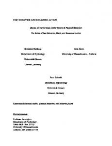
Latent Variables in a Travel Mode Choice Model... Explanatory Variables s, z

Latent Variables

η

Indicator Variables y

7

Latent Variable Model

Utility u

Choice d

Choice Model

Figure 1: Integrated Choice and Latent Variable Model (Ben-Akiva et al., 1999, p.195) preferences and individual preferences for flexibility and safety. Altogether we include five different latent variables in the choice model. The framework for modelling and estimation, adapted from Morikawa et al. (2002), consists of a latent variable model (MIMIC) and a discrete choice model. Both these models consist of structural and measurement equations.14 Figure 1, adapted from Ben-Akiva et al. (1999), gives a schematic picture of the modelling framework, where ellipses represent unobservable variables and rectangles observable variables. Dashed arrows represent measurement equations while solid arrows represent the structural equations. The latent variable model describes the relationships between the latent variables and their indicators and causes, while the discrete choice model explains modal choice. The complete, integrated choice and latent variable model explicitly incorporates latent variables in the choice process. The estimation is performed in two steps where the latent variable model is estimated first and then the discrete choice model is estimated. Although the estimation could be performed simultaneously, it is less cumbersome to estimate the model sequentially. The specification of the “multiple indicator part” (MI) of the MIMIC model was assisted by exploratory and confirmatory factor analyses performed in the LISREL software (Jöreskog and Sörbom, 1993). The resulting latent variable model presented here is, thus, the result of a search process involving both the unconditional search of relations between indicators and latent variables as well as several direct tests of postulated relationships (for 14 The measurement equations are also structural, in the sense that they describe structural relationships (Bollen, 1989, p.11).


8

exact model equations, see Appendix B).15 There are several ways of formulating discrete modal choice models, each emphasizing different aspects of modal choice (cf. Jara-Diaz and Videla, 1989; Train and McFadden, 1978; DeSerpa, 1971; Becker, 1965). The model used here is based on the fairly general disaggregate choice model by JaraDiaz (1998) and Jara-Diaz and Videla (1989). Generally, the conditional indirect utility uij for mode j (j ∈ J) for individual i is given by uij = u(Yi − pj, wij ) + ν ij , where Yi is the individual’s income, pj is the travel cost of mode j,16 wij is modal attributes and individual characteristics and ν ij is a random disturbance. Thus, the random utility is composed of a systematic term, which is a function of both latent and observable variables and a random disturbance, ν ij . In the empirical application we assume linear specifications of the conditional indirect utility function and of the latent variable functions. Suppressing individual indexation, the utility of travel mode j is uj = a0j s + b0 zj + c0j η + ν j ,

(1)

where zj is a vector of observable mode specific attributes (including travel cost), s a vector of observable individual specific attributes and η is a vector of individual specific latent variables. The structural relations to the latent variables are modelled as η = Γx + ζ. (2) The measurement equations are ½ j if uj ≥ uk ; ∀k ∈ J d= 0 otherwise

(3)

and y = Λη + ε.

(4)

In these equations, y is a vector of 20 observable indicator variables of η, x is a vector of six exogenous observable variables that cause η (x may or may not be a part of s), aj , b and cj are vectors of unknown parameters to be estimated and Γ and Λ are matrices of unknown parameters to be 15

After some trial models, the full MIMIC model was also, at the outset, estimated in LISREL with the WLS estimator (χ2 [df = 274] = 2541.7; RMSEA = 0.07; NNF I = 0.94; CF I = 0.95). Further information about the MIMIC model and the estimation method is given below and in Appendices B and C. 16 The budget constraint is Yi = G + pj , where G is a K × 1 column vector of consumed continuous goods and where Yi and pj are normalised by the price of G.


9

estimated and ν= (ν 1 , ..., ν J ), ζ and ε are measurement errors independent of s, zj and x (see Appendix B). Equations (1) and (3) form a discrete regression model, while equations (2) and (4) constitute the MIMIC model.

5

Results

5.1

The Latent Variable Model (MIMIC)

Based on the results from the factor analytic LISREL models (not reported), we postulate the existence of a safety personality trait and a environmental personality trait. While the safety personality trait is indicated by the respondent’s propensity to use safety gear when biking, boating and driving (y6 −y9 ), the environmental personality trait is indicated by the respondent’s composting and recycling habits (y1 − y5 ).17 The multiple indicator part of the model is a confirmatory factor analytical model specified such that we have five indicators for environmental preferences (η env ), four indicators for safety (η saf e ), comfort (η comf ) and convenience (ηconv ) and three for flexibility (η f lex ). The multiple causes part of the model is given by η li = γ l1 WOMANi + γ l2 AGEi + γ l3 INCOMEi + γ l4 KIDi + + γ l5 HOUSEi + γ l6 EDUCATIONi + ζ i , l = env, saf e, comf, conv, f lex That is, the causes for the individual’s latent preferences are the individual’s age (years), income, gender (equal to one if woman), the presence of children in the household (equal to one if there are persons younger than 18 years in the household), education (in years) and house tenure. Results from the first step maximum likelihood estimation are given in Tables 1 and 2.18 Evidently, all factor loadings in the measurement equations are positive and significant, which means that all indicators contribute to the construction of the latent preferences. Cronbach alpha values for the multiple indicator (MI) part of the MIMIC model are αηenv = 0.73, αηsaf e = 0.41, 17

All of these items are recycled without refunds and recycling is not mandatory. Collection points for recycling of glass and paper are abundant in Sweden and most grocery shops supply recycling containers for used nickel-cadmium batteries. Even though recycling is not mandatory, misapprehension or social norms seem to promote recycling (Paulsson et al., Dagens Nyheter 030210). As shown in section 2, we are aware of the fact that people may recycle for other than environmental reasons (and use bike helmets for other than safety reasons). Our hypothesis is just that environmentalism (safety) is one, among other, motives for these behaviours. 18 For details on the estimation, see Appendices B and D.


10

αηcomf = 0.76, αηconv = 0.71 and αηf lex = 0.73.19 According to Nunnally (1978), values of 0.70 are acceptable. Thus, αηsaf e seem to be unacceptably low. This could, however, be the result of individual heterogeneity, i.e. something that we control for in the full MIMIC model. Whereas Ben-Akiva et al. (1999) note that it sometimes can be difficult to find good causal variables for the latent variables, this does not seem to be the case here. Because the causal variables (as well as the indicator variables) are predictors of the latent variables, we retain the statistical significant (at the individual five percent level) causes and re-estimate the MIMIC model. These are the results presented in Tables 1 and 2. We find that women are more environmentally inclined (η env ) than men. This result seems logical considering the indicator variables underlying the construction of η env , i.e. composting kitchen refuse and recycling of glass, paper, batteries and metal, and the fact that women to a greater extent than men perform household recycling (Bennulf and Gilljam, 1991). The significance of age as a cause for η env is also consistent with a previous finding (Drottz-Sjöberg, 1997). Furthermore, higher incomes are coupled with stronger preferences for convenience (η conv ), potentially reflecting the fact that the opportunity cost of time losses is higher at higher incomes. A little surprising is that preferences for safety (η saf e ) decrease with income. However, this does not imply that safety is a non-normal good. Considering the indicators used to construct safety preferences, this merely shows that respondents with higher incomes use safety gear and adhere to speed limits to a lesser extent than respondents with lower incomes. Finally, considering the indicators used to construct flexibility (η f lex ) it seems natural that respondents with children have stronger preferences for flexibility. Table A2 in Appendix A gives the model predicted mean values of the ∧ latent variables (η k ), stratified by the chosen mode. Train users have a ∧ significantly larger mean η env value than car and bus users. Car users have ∧ ∧ a significantly lower mean value of η saf e and η conv than train users. Car users ∧

have a significantly lower mean value of ηcomf than bus users who have a ∧

significantly lower mean value of η comf than train users. Furthermore, car ∧

users have a higher mean value of ηf lex than bus and train users. Thus, the predicted values of the latent variables are in several cases significantly different for the different modes. 19

Cronbach’s alpha assesses the reliability in the measurement of an unobserved factor (Stata Reference Manual Release 7, 2001). The alpha values given here are based on standardised indicator variables.


5.2

11

The Discrete Choice Model

When it comes to the parameters of the choice model, we hypothesize that the generic parameters for time and cost will be negative so that the mode’s likelihood of being chosen decreases when modal cost and time increase. We also postulate that the need to use own car in work (OWN) and having a car available for the worktrip (AVAIL) will increase the probability of choosing car over train and bus. Apart from differing times and costs, the different modes also have different objective probabilities of death and injury as well as different objective energy consumption and emissions. It is, therefore, possible, with a few additional assumptions, to objectively tell which mode is the most (least) risky as well as the most (least) environmentally friendly. For the latent variables comfort, convenience and flexibility we are unable to give objective orderings of the modes, i.e. we can not on any objective grounds tell which is the most comfortable mode. Considering environmental friendliness, Lenner (1993) has calculated emission equivalents per person and energy consumption equivalents per person for car, bus and train. Based on Lenner’s results, we postulate that respondents with environmental preferences will choose train over bus and bus over car.20 On the relevant stretch of the motorway (the “E4”) between Uppsala and Stockholm, car has considerable higher historical, objective, risks of death and injury compared to bus and train. Between January 1998 and January 2003, six people have been killed in car accidents and none in bus accidents (Swedish National Road Administration, pers. comm.). Despite the real number of deaths, the historical probabilities of being killed in car and bus accidents on this particular stretch of road are very small, especially considering the number of vehicles and people travelling there. Even though the difference in risk between bus and car is large, the baseline risks are still very small.21 Thus, it is possible that the differences in modal safety are too small to be discernible. For the parameters of the other latent variables (ccomf − cf lex ), we base our hypotheses about the parameters on the indicator variables used to construct the individual preferences (see Appendix B). For comfort (ccomf ), we postulate that individuals with preferences for comfort will choose train over bus and bus over car, since the comfort of train is larger that of bus and the comfort of bus is larger than that of car - proviso the indicator variables used for comfort. Furthermore, we hypothesize that car provides greater flexibility (cf lex ) than bus and train (with no significant difference 20 Lenner (1993) shows that, under Swedish conditions, electricity driven trains have lower energy consumption and produce less emissions than petrol/diesel driven buses. 21 Anecdotal evidence based on personal communication with employees at the SNRA suggests that this stretch of the motorway is the safest in Sweden.


12

between the latter). We have no hypotheses about the convenience (cconv ) parameter. In Table 3 the results from a multinomial probit models with and without latent variables (M N PLV E and M N PREF , respectively) are given.22 A likelihood ratio test between the two models results in a test statistic of 255.3, which, with 10 degrees of freedom23 , strongly rejects the null hypothesis of the reference model without latent variables ( M N PREF ).24 Furthermore, the Akaike information criterion (AIC) - a means for comparing non-nested models - with number of parameters equal to the sum of the MIMIC and M N PLV E parameters is smaller for the latent variables enriched model than for the reference model. Below we first comment on the modal and socioeconomic variables, thereafter we provide a longer discussion on the latent variables, η. Economizing on space, we will mainly comment on results that we find particularly interesting. 5.2.1

Modal and Socioeconomic Variables

Most of the common variables that are significant in the reference choice model are also significant in the latent variables enriched discrete choice model. However, there are a few exceptions. For instance, in the reference choice model, the presence of children in the household increases the likelihood of choosing car over bus. This relationship is insignificant in the latent variables enriched discrete choice model. Presumably the preferences captured by the variable KID in the reference choice model is better captured by the latent variables in the enriched discrete choice model. Turning to the traditional modal choice variables, travel time and travel cost, we find that both are significant with the expected signs in both the reference choice model and in the latent variables enriched discrete choice model. The value of time (VOT) from the reference choice model is SEK 224, while the value of time in the latent variables enriched discrete choice model is SEK 175. The VOT is still very high compared to the official value of SEK 42 for private travels of less than 100 kilometers (SIKA, 2002), a 22

b Based on the estimates from the MIMIC model we formulate the predicted values of η b (the conditional covariance of η) (see Appendix D for details). The discrete choice and Υ model is then estimated (employing these predicted values) using a multinomial probit ML estimator with varying choice sets. Since we include predicted values of η in place of the unknown values in the discrete choice model (see e.g. Murphy and Topel, 1985; Pagan, 1986), we correct the standard ML covariance matrix estimator (see equation (16) in Appendix D). 23 This LR test is not strictly correct, since we neglect the indicators and causes used to construct the latent variables in the MIMIC model. However, it can still be taken as evidence of the benefit of using latent variables as determinants in the modal choice model. 24 A less restrictive, random parameters probit, model in which the modal time and cost parameters were allowed to vary across the respondent was also estimated (ln = −413.6). The Akaike information criterion (AIC) for this model is equal to 1.07.


13

fact potentially explained by the higher incomes in our sample and/or by the fact that a number of respondents have to make one or more modal changes.25 5.2.2

Latent Variables

Turning to the latent variables, we find that two latent variables are significant at the five percent level (ccomf,CAR , cf lex,CAR ) in the choice between car and bus. In the choice between train and bus one latent variable is significant at the five percent level (ccomf,T RAIN ) while another is significant at the ten percent level (cenv,T RAIN ). Thus, preferences for comfort increase the likelihood of choosing bus over car (ccomf,CAR ) and train over bus (ccomf,T RAIN ). This is consistent with our hypothesis and is hardly surprising considering the indicator variables used to construct the comfort variable, i.e. the respondent’s attitudes towards travelling in a non-noisy, environment with possibilities of resting, working and moving around. Preferences for flexibility increase the likelihood of choosing car over bus (cf lex,CAR ) which also is consistent with our hypothesis and reasonable considering the indicators used to construct the flexibility variable: the need to shop, run errands or leave or collect children on the way to and from work. Consistent with our hypothesis, we find that environmental preferences (cenv,T RAIN ) increase the likelihood of choosing train over bus. Interesting to note is that safety, the latent variable with the lowest Cronbach alpha value in the factor analytic model, is insignificant in both the choice between car and bus and in the choice between train and bus. If the low Cronbach alpha value can not be explained by individual heterogeneity (as is done in the MIMIC model), it is possible that the indicators used are not well suited for capturing the latent variable we would like to model. For instance, if the safety variable constitutes a mixture of preferences for personal (security) and traffic safety, it is not surprising that the individuals’ safety values (stratified by mode) are more similar than they would be if traffic safety and personal safety were independent constructions. This follows naturally from the assumption that the personal and traffic safety effects work in opposite directions, i.e. car is low on traffic safety and high on personal safety whereas public modes are high on traffic safety and low on personal safety. 25 The average Swedish pre-tax household income in 2001 was SEK 23,506 per month (HE 20 SM 0201). The value of time during modal changes is twice the value of time when travelling (SEK 84) (SIKA, 2002). As a reference to these values, the average hourly earnings in the private sector (excluding overtime) was SEK 108 in october 2001 (AM SM 38 0201).


6

14

Conclusions

In a commute context, we use survey data to construct and test the significance of five individual specific latent variables postulated to be important for modal choice: environmental preferences, safety, comfort, convenience and flexibility. On several accounts our “latent variables enriched” choice model outperforms a traditional choice model and provides insights into the importance of unobservable variables in modal choice. Our latent variables enriched choice model also turns out to be superior to a random parameters model where modal time and cost are allowed to vary. In general, our results confirm that modal time and cost are significant for modal choice but also show that preferences for flexibility and comfort are very important. According to expectation, environmental preferences increase the likelihood of choosing an environmentally friendly mode, train, over a less environmentally friendly mode, bus. Environmental preferences do, however, not matter in the choice between car and bus. If the government’s goals for an environmentally sustainable and safe transport sector is to be achieved (Gov. Bill 1997/98:56), policy makers have to understand what prevents individuals from making environmentally sounder transport choices. Based on our results, we believe the policy challenge lies in reducing the welfare loss from behaving environmentally. Given the existing vehicle fleet, there are two possible ways (or a combination thereof) of doing this: either public modes become more “private” through, for instance, increased levels of flexibility or car becomes more expensive and cumbersome to use. In the future, fuel cell or other technology may reduce motorism’s adverse environmental effects. Congestion problems are, however, likely to remain unless individuals have incentives to change from private to public modes. Interesting to note is that preferences for safety are insignificant in the present modal choice model. This does not necessarily mean that safety considerations are unimportant in modal choice in general. Because the base line risks are very small in the commute under study here, the risks are perhaps too small to be discernible to the respondents. Furthermore, since the safety variable has low construct reliability, we may not fully measure what we intend to measure. An interesting issue for future research would be to investigate whether the form of safety (traffic safety, personal safety et cetera) preferences varies systematically with the trip characteristics, i.e. whether the trip is long or short, performed once or repeatedly, at work or leisure, within a city or in the countryside and so on. Should such differences be significant, the VOSL used in SNRA’s cost benefit analyses should arguably be adjusted and differentiated accordingly. Differentiated VOSL which better capture individuals’ preferences for safety is also desired from a policy perspective (SIKA, 2002). Thus, elicitation methods should


15

be designed to elicit individuals’ preferences for different forms of safety under varying circumstances (e.g. trip length, trip purpose, initial risk level, geographical location). Because the construct reliability of the attitudinal latent variables was on average higher than the construct reliability of the behavioural latent variables, a tentative conclusion is that preferences constructed from attitudinal indicators are to be preferred over preferences constructed from behavioural indicators. Because it is easier to find suitable attitudinal than behavioural indicator variables, attitudinal indicator variables may also be preferred on practical grounds. Nonetheless, an indisputable advantage of behavioural indicator variables over attitudinal is that they are exogenous to modal choice. Notwithstanding the mixed results of this pioneering survey, we still believe that a carefully constructed battery of behavioural questions have a great potential in capturing the individual’s latent preferences. Future research will put our belief at test.


ˆ matrix of Table 1: The Λ Indicator η env Compost (y 1 ) 1 1.65 (15.1) Glass (y 2 ) 1.30 (14.1) Paper (y 3 ) 1.45 (14.8) Battery (y 4 ) 1.08 (13.7) Metal (y 5 ) Bikehelm (y 6 ) Speedlim (y 7 ) Lifejacket (y 8 ) Safebelt (y 9 ) Calmenv (y 10 ) Rest (y 11 ) Move (y 12 ) Work (y 13 ) Nowait (y 14 ) Knowtime (y 15 ) Novarian (y 16 ) Noqueues (y 17 ) Shop (y 18 ) Leavekid (y 19 ) Drivekid (y 20 )

16

factor loadings (t-statistics in parentheses). η saf e ηcomf η conv η f lex

1 1.67 (5.24) 1.37 (7.29) 1.22 (6.42) 1 1.43 (20.7) 0.97 (16.9) 1.12 (18.3) 1 1.79 (18.4) 1.53 (17.9) 0.76 (12.0) 1 2.88 (12.6) 2.63 (12.8)

Note: Indicator and variable definitions are given in Appendix B.

ˆ matrix (t-statistics in parentheses). Table 2: The Γ WOMAN

η env η saf e η comf η conv η f lex

AGE

0.030 (2.36) 0.114 (7.21)

0.112 (7.89) 0.083 (5.51)

0.066 (4.40)

0.059 (3.68)

0.102 (7.42) -

-0.065 (-7.76)

INCOME

KID

-0.042 (-2.95)

HOUSE

EDUCATION

0.041 (3.25) 0.031 (2.77)

-

0.042 (3.24)

-

-

-0.099 (-6.20)

0.191 (11.40)

0.053 (4.00) -

0.186 (11.80)

-

-

Note: Variable definitions are given in Appendix B.


17

Table 3: MNP estimations of the reference and latent variables enriched models. MNPREF Variables/Parameters TIME COST

αCAR WOMANCAR AGECAR KIDCAR EDUCATIONCAR HOUSECAR DCOMCAR OWNCAR AVAILCAR

ηenv,CAR ηsaf e,CAR ηcomf,CAR ηconv,CAR ηf lex,CAR αT RAIN WOMANT RAIN AGET RAIN KIDT RAIN EDUCATIONT RAIN HOUSET RAIN DCOMT RAIN OWNT RAIN AVAILT RAIN

ηenv,T RAIN ηsaf e,T RAIN ηcomf,T RAIN ηconv,T RAIN ηf lex,T RAIN n ln LRI AIC

MNPLV E

Estimate

t-statistic

Estimate

t-statistic

-0.61 -0.23 -2.06 -0.20 -0.00 0.34 0.04 0.04 0.05 1.07 1.83

-10.66 -4.98 -3.37 -1.30 -0.64 2.18 1.67 0.25 0.57 3.63 8.11

-1.07 -0.51 -6.77 -0.69 0.01 0.07 0.17 -0.01 0.15 2.67 4.07 -0.02

-6.82 -3.70 -3.77 -1.44 0.45 0.15 2.76 -0.02 0.72 3.27 5.12 -0.03

1.27

1.24

-3.68

-5.91

0.24

0.55

2.46

2.84

-1.20 -0.83 -0.02 0.43 0.16 -0.82 0.00 -0.37 0.24 0.70

-0.93 -2.20 -1.13 1.12 3.18 -1.47 0.02 -0.42 0.81 1.86

0.72

0.76

1.22

2.45

-1.07 -0.14 -0.00 0.20 0.11 -0.14 0.00 -0.13 0.13

811 -453.49 0.33 1.17

-1.76 -0.89 -0.28 1.28 4.60 -0.82 0.03 -0.38 0.79

0.60

1.60

-0.16

-0.24

811 -325.84 0.52 0.94

Note: The likelihood ratio index, LRI = 1 − (ln / ln 0 ). ln 0 is the log likelihood only with a constant term (Greene, 1993, ch.21). 2p

2 The Akaike information criterion, AIC = − n ln + n , where p is the number of parameters and n the sample size (Amemiya, 1985).


18

References Amemiya, T. (1985): Advanced Econometrics. Harvard University Press, Cambridge Ajzen, I. and Fishbein, M. (1980): Understanding Attitudes and Predicting Social Behavior. Prentice-Hall, Inc., Englewood Cliffs, New Jersey AM SM 38 0201: Konjunkturstatistik, löner för privat sektor under oktober 2001. Statistics Sweden (2002). In Swedish with a summary in English. Andreoni, J. (1989): Giving with Impure Altruism: Applications to Charity and Ricardian Equivalence. Journal of Political Economy, 97, 144758 Ashok, K., Dillon, W. R. and Yuan, S. (2002): Extending Discrete Choice Models to Incorporate Attitudinal and Other Latent Variables. Journal of Marketing Research, XXXIX, 31-46 Becker, G. S. (1965): A Theory of the Allocation of Time, The Economic Journal, 75, 493-517 Ben-Akiva, M., McFadden, D., Gärling, T., Gopinath, D., Walker, J., Bolduc, D., Börsch-Supan, A., Delquié, P., Larichev, O., Morikawa, T., Polydoropoulou, A., Rao, V. (1999): Extended Framework for Modeling Choice Behavior. Marketing Letters, 10(3), 187-203 Bennulf, M. and Gilljam, M. (1991): Snacka går ju - men vem handlar miljövänligt? In Weibull, L. and Holmberg, S. (eds.) Åsikter om massmedier och samhälle. SOM undersökningen 1990, SOM Rapport 7. In Swedish. Bollen, K. A. (1989): Structural Equations with Latent Variables. John Wiley and Sons, Inc. Browne, M. W. (1984): Asymptotically Distribution Free Methods for the Analysis of Covariance Structures. British Journal of Mathematical and Statistical Psychology, 37, 62-83 Browne, M. W. and Cudeck, R. (1993): Alternative Ways of Assessing Model Fit. In Bollen, K. A. and Long, J. S. (eds.): Testing Structural Equation Models. Newbury Park, CA, Sage, 136-162 Daniels, R. F. and Hensher, D. A. (2000): Valuation of Environmental Impacts of Transport Projects. The Challenge of Self-Interest Proximity. Journal of Transport Economics and Policy, 34(2), 189-214 DeSerpa, A. C. (1971): A Theory of the Economics of Time. The Economic Journal, 81, 828-846 Diamond, P. A. and Hausman, J. A. (1994): Contingent Valuation: Is Some Number better than No Number? The Journal of Economic Perspectives, 8(4), 45-64 Drottz-Sjöberg, B-M. (1997): Attitudes, Values and Environmentally Adapted Products. Rhizikon Report No 30, Stockholm School of Economics


19

Dunlap, R. E. and van Liere, K. D. (1978): The New Environmental Paradigm. The Journal of Environmental Education, 9, 10-19 Dunlap, R. E., van Liere, K. D., Mertig, A. G. and Jones, R. E. (2000): Measuring Endorsement of the New Environmental Paradigm: A Revised NEP scale. Journal of Social Issues, 56(3), 425-442 Gov. Bill 1997/98:56: Transportpolitik för en hållbar utveckling. Regeringens proposition 1997/98:56. In Swedish. Greene, W. H. (1993): Econometric Analysis. 2nd edition, Macmillan, New York Hammit, J. K. and Graham, J. D. (1999): Willingness to Pay for Health Protection: Inadequate Sensitivity to Probability? Journal of Risk and Uncertainty, 18, 33-62 Hausman, J. A. and Wise, D. A. (1978): A Conditional Probit Model for Qualitative Choice: Discrete Decisions Recognizing Interdependence and Heterogenous Preferences. Econometrica, 46(2), 403-426 HE 20 SM 0201: Inkomster, skatter och bidrag 2000. Individ- och familjeuppgifter, Statistics Sweden (2002). In Swedish with a summary in English. Hu, L-T. and Bentler, P. M. (1995): Evaluating Model Fit. In Rick H. Hoyle (ed.): Structural Equation Modelling. Concepts, Issues and Applications. Sage Publications Inc., 76-99 Jara-Diaz, S. R. (1998): Time and Income in Travel Choice: Towards a Microeconomic Activity-Based Theoretical Framework. In Gärling, T., Laitila, T. and Westin, K. (eds.): Theoretical Foundations in Travel Choice Modeling. Pergamon Jara-Diaz, S. R. and Videla, J. (1989): Detection of Income Effect in Mode Choice: Theory and Application. Transportation Research, 23B, 393400 Jones-Lee, M. W., Hammerton, M. and Philips, P.R. (1985): The Value of Safety: Results from a National Sample Survey. Economic Journal, 95, 49-72 Jöreskog, K. G. and Sörbom, D. (1996): LISREL 8: User’s Reference Guide, Scientific Software International, Inc., Chicago Kahneman, D. and Knetsch, J. L. (1992): Valuing Public Goods: The Purchase of Moral Satisfaction. Journal of Environmental Economics and Management, 22, 57-70 Krantz Lindgren, P. (2001): Att färdas som man lär? Om miljömedvetenhet och bilåkande. Gidlunds förlag, Hedemora. In Swedish. Lenner, M. (1993): Energy Consumption and Exhaust Emissions Regarding Different Means and Modes of Transportation. VTI Meddelande nr 718 (in Swedish with a summary in English) Länsstyrelsen Uppsala län (2002): Fakta om Uppsala län. Mini uppslagsboken 2002-2003. In Swedish.


20

McFadden, D. (1986): The Choice Theory Approach to Market Research. Marketing Science, 5(4), 275-297 Morikawa, T., Ben-Akiva, M. and McFadden, D. (2002): Discrete Choice Models Incorporating Revealed Preferences and Psychometric Data. Econometric Models in Marketing Advances in Econometrics: A Research Annual, 16, 27-53, Elsevier Science Ltd. Morikawa, T. and Sasaki, K. (1998): Discrete Choice Models with Latent Variables Using Subjective Data. In Ortúzar, J de D., Hensher, D. A. and Jara-Diaz, S.: Travel Behaviour Research: Updating the State of Play, 435-455, Pergamon, Oxford Murphy, K. and Topel, R. (1985): Estimation and Inference in Two Step Econometric Models. Journal of Business and Economic Statistics, 3, 370-379. Naturvårdsverket (1996): Biff och Bil? Om Hushållens Miljöval, Report 4542. In Swedish. Naturvårdsverket (2003): Värdering av tid, olyckor och miljö vid väginvesteringar. Kartläggning och modellbeskrivning. Rapport 5270. In Swedish. Nunnally, J. C. (1978): Psychometric Theory. Second edition. McGrawHill, New York Ortúzar, J. de D. and Willumsen, L. G. (1999): Modelling Transport. Second edition. John Wiley and Sons, New York Oskamp, S., Harrington, M. J., Edwards, T. C., Sherwood, D. L., Okuda, S. M. and Swanson D. C. (1991): Factors Influencing Household Recycling Behavior. Environment and Behavior, 23(4), 494-519 Pagan, A. (1986): Two Stage and Related Estimators and Their Applications. Review of Economic Studies, LIII, 517-538 Paulsson, V., Norrby, S., Mellbin, K-G, Selberg, P., Löfstedt, L.: Bättre för miljön att inte sopsortera. Dagens Nyheter 030210. In Swedish. Pearce, D. (1998): Cost-Benefit Analysis and Environmental Policy. Oxford Review of Economic Policy, 14(4): 84-100 Pendleton, L. H. and Shonkwiler, J. S. (2001): Valuing Bundled Attributes: A Latent Characteristics Approach. Land Economics, 77(1): 118-129 Persson, U., Nilsson, K., Hjalte, K. and Norinder, A. (1998): Beräkning av Vägverkets riskvärden. En kombination av “contingent valuation”skattningar och uppmätta hälsoförluster hos vägtrafikskadade personer behandlade vid fyra sjukhus. The Swedish Institute of Health Economics (IHE), mimeo. Satorra, A. and Bentler, P. M. (1988): Scaling corrections for chi-square statistics in covariance structure analysis. Proceedings of the Business and Economic Statistics Section of the American Statistical Association, 36, 308-313. SIKA (2002): Översyn av samhällsekonomiska metoder och kalkylvärden på transportområdet - ASEK. SIKA Rapport 2002:4. In Swedish.


21

Review of cost benefit calculation. Methods and valuations in the transport sector. SIKA. Smith, V. K. and Desvousges, W. (1987): An Empirical Analysis of the Economic Value of Risk Changes. Journal of Political Economy, 95, 89-114 Stata Reference Manual Release 7 (2001), Stata Statistical Software, Stata Press, College Station Stern, P. C. and Oskamp, S. (1987): Managing Scarce Environmental Resources. In Stokols D. and I. Altman (eds.): Handbook of Environmental Psychology, vol. 2, 1043-1088. Wiley and Sons, New York Train, K.A. and McFadden D. (1978): The Goods/Leisure Tradeoff and Disaggregate Work Trip Mode Choice Models. Transportation Research, 12(5), 349-353 Vredin Johansson, M. (1999): Using Modal Perceptions to Determine Work Trip Travel Mode. In Vredin Johansson, M.: Economics Without Markets: Four Papers on the Contingent Valuation and Stated Preference Methods. Umeå Economic Studies No.517. Umeå University Press West, S. G., Finch, J. F. and Curran, P. J. (1995): Structural Equation Models with Nonnormal Variables. Problems and Remedies. In Hoyle, R. H. (ed.): Structural Equation Modelling. Concepts, Issues and Applications. Sage


22

Appendix A: Descriptive Statistics Table A1: Descriptive statistics: total and analytic sample. ∧ Means (µ), standard errors (SE) and number of observations (n). Total sample Variable Gender (Woman=1) Age (years) Education (years) Household income (SEK) Children Travel time (minutes)a Travel cost (SEK)a Commuting days per week House tenure

Analytic sample

∧

µ

SE

n

µ

∧

SE

n

0.33 43.20 14.52 43,100 0.47 57.57 73.45 4.58 0.49

0.01 0.26 0.09 438 0.01 0.55 3.07 0.02 0.01

1,706 1,706 1,697 1,688 1,678 1,683 1,686 1,690 1,683

0.35 42.77 14,91 44,994 0.49 59.39 72.62 4.56 0.45

0.02 0.37 0.13 630 0.02 0.79 1.72 0.03 0.02

811 811 811 811 811 811 811 811 811

a Mean travel time and cost are given for the chosen modes.


23

Table A2: Descriptive statistics: analytic sample stratified by mode. ∧ Means (µ), standard errors (SE) and number of observations (n). Car (n

Train (n

SE

µ

0.29 42.67 14.30 46,022 0.55 46.39 95.27 4.58 0.52

0.02 0.50 0.18 903 0.02 0.78 2.93 0.04 0.02

ηenv ∧ ηsaf e

-0.02

∧ ∧

= 309)

Bus (n

= 96)

SE

∧

µ

SE

0.40 43.35 16.17 46,545 0.43 74.58 55.84 4.53 0.39

0.03 0.61 0.19 997 0.03 1.07 0.72 0.06 0.03

0.45 41.32 13.47 35,651 0.40 65.44 30.81 4.51 0.36

0.05 1.16 0.35 1,576 0.05 2.48 1.45 0.08 0.05

0.02

0.07

0.02

-0.07

0.05

-0.01

0.01

0.03

0.01

0.01

0.02

ηcomf

-0.32

0.02

0.40

0.02

0.11

0.03

ηconv ∧ ηf lex

-0.04

0.02

0.08

0.02

-0.05

0.05

0.07

0.02

-0.07

0.02

-0.08

0.03

Gender (Woman=1) Age (years) Education (years) Household income (SEK) Children Travel time (minutes) Travel cost (SEK) Commuting days per week House tenure ∧

µ

= 406)

∧

Variable

∧


24

Appendix B: Variables and Equations Table B1: Latent and model variables. Variable

Definition


Environmental preferences (latent variable). Safety (latent variable).

WOMAN

Dummy variable for the gender of the respondent with one for female respondents. The age of the respondent in years. The income of the respondent in SEK. Dummy variable with value one if the respondent’s household includes children (persons younger than 19 years). Dummy variable with value one if the respondent has house tenure. Travel time in minutes. Travel cost in SEK. The respondent’s education in years. Number of days the respondent commutes per week. Dummy variable equal to one for the need to use own car in work at least one day a week. Dummy variable equal to one for the availability of a car for worktrips at least one day a week.

AGE INCOME KID HOUSE TIME COST EDUCATION DCOM OWN AVAIL

Comfort (latent variable). Convenience (latent variable). Flexibility (latent variable).


25

Table B2: Indicator variables. Indicator Variable

y1 y2

Compost Glass

y3 y4 y5 y6

Paper Battery Metal Bikehelm

y7

Speedlim

y8

Lifejacket

y9

Safebelt

y10

Calmenv

y11

Rest

y12

Move

y13

Work

y14

Nowait

y15

Knowtime

y16

Novarian

y17

Noqueues

y18

Shop

y19

Leavekid

y20

Drivekid

Definition The respondent’s habit of composting kitchen refuse. The respondent’s habit of recycling non deposit-refund glass bottles, jars et cetera. The respondent’s habit of recycling newspapers and paper. The respondent’s habit of recycling batteries. The respondent’s habit of recycling metal. The respondent’s habit of wearing a bike helmet when riding a bike. The respondent’s habit of adhering to prevailing speedlimit when driving. The respondent’s habit of using a life jacket when in smaller boats. The respondent’s habit of using safety belts in cars (also in the rear seats). The respondent’s appreciation of travelling in a calm, non-noisy environment. The respondent’s appreciation of being able to rest or read while travelling to/from work. The respondent’s appreciation of being able to move around while travelling to/from work. The respondent’s appreciation of being able to work while travelling to/from work. The respondent’s appreciation of not having to wait for another travel mode while travelling to/from work. The respondent’s appreciation of knowing how long the daily travel time to/from work is. The respondent’s appreciation of having little or no variation in her daily travel time to/from work. The respondent’s appreciation of avoiding queues and congestion while travelling to/from work. The respondent’s appreciation of being able to shop or run errands while travelling to/from work. The respondent’s appreciation of being able to leave/collect children at school or similar while travelling to/from work. The respondent’s appreciation of being able to give children a ride to their leisure time activities while travelling to/from work.


26

The first nine indicator variables (y1 −y9 ) are measured on five point category scales scored between Never and Always. All other indicator variables (y10 − y20 ) are measured on five point semantic differential scales with the endanchors Not important at all and Very important. Equation (2): η = Γx + ζ       WOMAN   η env γ 11 γ 12 γ 13 γ 14 γ 15 γ 16  ζ 1    ζ2   η saf e   γ 21 γ 22 γ 23 γ 24 γ 25 γ 26   AGE       INCOME   + ζ 3   η comf  =  γ 31 γ 32 γ 33 γ 34 γ 35 γ 36         KID     ζ   η conv   γ 41 γ 42 γ 43 γ 44 γ 45 γ 46   4  EDUCATION  γ 51 γ 52 γ 53 γ 54 γ 55 γ 56 ζ5 η f lex HOUSE

Equation (4):

y = Λη + ε                                     

y1 y2 y3 y4 y5 y6 y7 y8 y9 y10 y11 y12 y13 y14 y15 y16 y17 y18 y19 y20





                                    =                                  

1 λ21 λ31 λ41 λ51 0 0 0 0 0 0 0 0 0 0 0 0 0 0

0 0 0 0

0 0 0 0

0 0 0 0

0 0 0 0

1 λ72 0 0 0 0 0 0 λ82 0 0 0 λ92 0 1 0 0 0 0 0 λ113 0 λ123 0 0 0 0 0 λ133 0 0 1 0 0 0 0 λ154 0 0 0 λ164 0 0 0 λ174 0 0 0 1 0 0 0 λ195 0 0 0 λ205





                                   


                    +                    

ε1 ε2 ε3 ε4 ε5 ε6 ε7 ε8 ε9 ε10 ε11 ε12 ε13 ε14 ε15 ε16 ε17 ε18 ε19 ε20

                                    


27

Appendix C: MIMIC Model Estimation Estimation of a structural equation latent variable model minimizes the difference between the sample covariance matrix, S, and the covariance matrix, Σ. The elements of Σ are hypothesized to be a function of the parameter vector θ so that Σ = Σ(θ). The parameters are estimated so that the discrepancy between S and the implied (by the parameters) covariance matrix ∧

Σ(θ) is minimal. The discrepancy function, F = F (S, Σ(θ)), measures the ∧

discrepancy between S and Σ(θ) evaluated at θ. Fmin is the minimum value ∧

of the discrepancy function and equals zero only if S =Σ(θ). An indication of model fit is, therefore, given by the closeness of the Fmin to zero (Browne and Cudeck, 1993). To test the model, the test statistic T = (N − 1)Fmin is calculated. If the model holds and is identified, T is asymptotically χ2 distributed. This test statistic, T , is often referred to as “the χ2 test” (Hu and Bentler, 1995)26 . However, the χ2 test statistic for overall model fit is vulnerable to sample size and departures from multivariate normality of the variables. If sample size is small, T might not be χ2 distributed and, if sample size is large, even a trivial model misspecification results in model rejection. Therefore, there are several supplementary fit indices available for assessing model fit (Hu and Bentler, 1995; Browne and Cudeck, 1993; Jöreskog and Sörbom, 1993). There are several different iterative estimation methods for structural equation models; unweighted least squares (ULS), generalized least squares (GLS), maximum likelihood (ML) and others (Jöreskog and Sörbom, 1993)27 . The most commonly used estimators, ML and GLS, assume that the measured variables are continuous and multivariate normally distributed. However, if the data are highly non-normal, ML and GLS produce inflated χ2 values and underestimate the standard errors of the parameters (West, Finch and Curran, 1995). An alternative estimator in the case of non-normality is the asymptotically distribution free weighted least squares estimator (ADFWLS or WLS) developed by Browne (1984). Under normality, the WLS estimator is equivalent to ML but, under non-normality, it produces asymptotically unbiased estimates of the χ2 test statistic and the standard errors. However, since the WLS estimator requires estimates of fourth-order moments28 , the WLS is of limited practical relevance when the sample size is small (West, Finch and Curran, 1995). When the variables are non-normal and the sample size is small29 , an alternative is to use ML with a correction 26

The χ2 test is in fact a “badness-of-fit” measure since small values correspond to good fit and large values correspond to bad fit (Jöreskog and Sörbom, 1993). 27 Discrepancy functions for the different estimators are ¤given in Bollen, 1989. £ 28 The fourth-order moment, kurtosis, m4 = E (x − µ)4 . 29 Depending on the model’s complexity, a small sample can consists of 1,000-5,000 cases (West, Finch and Curran, 1995).


28

of the χ2 statistic. This correction, the Satorra-Bentler correction (Satorra and Bentler, 1988), re-scales the normal-theory χ2 statistic to account for non-normality (multivariate kurtosis) and holds regardless of the distribution of the variables (Hu and Bentler, 1995). The Satorra-Bentler correction also produces robust standard errors. In our data, the majority of the variables clearly depart from normality since they consists of ordinal indicator variables. When testing the more continuous variables30 for normality, all proved significant kurtosis and skew. Therefore, we estimate the model with WLS.

30

These variables are; the AGE of the respondent (a truncated variable), the INCOME of the respondent (a categorised variable) and the respondent’s EDUCATION in years.


29

Appendix D: Full Model Estimation The structural equations consist of the four measurement and structural equations ((1)-(4)) given in Section 3 (repeated here for convenience) uj = a0j s + b0 zj + c0j η + ν j ,

(5)

η = Γx + ζ.

(6)

d= and

½

j if uj ≥ uk ; ∀k ∈ J 0 otherwise

(7)

y = Λη + ε.

(8)

y is a (q × 1) vector of observable indicators of η, s and zj are vectors of observable exogenous variables (zj is mode specific, while s is individual specific), η is a (l × 1) vector of individual latent variables, x is a (k × 1) vector of exogenous observable variables that cause η (x may or may not be a part of s), aj , b and cj are vectors of unknown parameters to be estimated and Γ and Λ are, respectively, (l × k) and (q × l) matrices of unknown parameters to be estimated and ν= (ν 1 , ..., ν J ), ζ and ε are measurement errors independent of s, zj and x and E(νν 0 ) = Ξ, E(εε0 ) = Θ, E(ζζ 0 ) = Ψ and E(νε0 ) = E(νζ 0 ) = E(εζ 0 ) = 0. Let u = (u1 , ...uJ )0 . Then we can write the J utilities above as u = As + Zb + Cη + ν, where



  a01  a02   , Z =  A=  ...   0 aJ

  z01  z02   and C =   ...  0 zJ

(9)  c01 c02   ...  c0J

For identification we let aJ = cJ = 0. Assume for the moment that the vector q = (y0 , η 0 , u0 )0 is multivariate normal with mean m1 and covariance matrix Ω1 , hence     ΛΨ ΛΨC0 ΛΓx Ω11 ,  and Ω1 =  ΨΛ0 m1 =  Ψ ΨC0 Γx 0 0 CΨΛ CΨ Ξ + CΨC As + Zb + CΓx

where Ω11 = ΛΨΛ0 + Θ. Let φ be the vector of parameters given in m1 and Ω1 above and let d be an indicator variable taking value one in row j if d = j then the likelihood for φ, for a sample of n individuals, is (φ) =

n X i=1

di ln Pr(di = j, yi |xi , si , zij ),

(10)


30

where Pr(di = 1, yi |xi , si , zij ) =

Z

...

η env

Z

η f lex

· R ∞ R ui1

R ui1 −∞ −∞ .... −∞ f (ui1 , ..., uiJ )dui1 , ..., duiJ

where f is a J variate normal density. Maximum likelihood estimation of φ is difficult and we do not pursue this here, instead we use a two step estimator (see e.g. Murphy and Topel, 1985; Pagan, 1986) for the model parameters. Conditional on y the distribution of the unobservables q2 = (η 0 , u0 )0 is multivariate normal with mean m2 = (E(η|y, x)0 , E(u|y, x, Z, s)0 ) and covariance matrix ¸ · Υ ΥC0 . Ω2 = CΥ Ξ + CΥC0 where Υ = Ψ − ΨΛ0 Ω−1 11 ΛΨ.

(11)

E(η|y, x) = Γx + ΨΛ0 Ω−1 11 (y − ΛΓx)

(12)

Here and E(u|y, x, Z, s) = As + Zb + CE(η|y, x) and hence we can write the utility functions (9) above as u = As + Zb + CE(η|y, x) + ϑ

(13)

where ϑ = Ce + ν and e = η−E(η|y, x). Thus Var(ϑ) = Ξ + CΥC0 . Divide the parameter vector φ into a parameter vector φ1 for the MIMIC model (i.e. Equations (2) and (4)) and a parameter vector φ2 describing the 0 0 b discrete choice model, thus φ = (φ1 , φ2 )0 . Now for a given value of φ1 = φ 1 the log-likelihood for φ2 , under random sampling, is X b di ln Pr(di = j|xi , yi , si , zij ), (14) 2 (φ2 ; φ1 ) = i=1

where

Pr(di = 1|xi , yi , si1 ) =

Z

∞

−∞

Z

ui1

−∞

....

Z

ui1

f (ui1 , ..., uiJ )dui1 ...duiJ ,

(15)

−∞

b 1 )+ϑij uij = a0j s + b0 zj + c0j E(η|y, x, φ

Observe that ϑij = ν ij + c0j e and hence

E(ϑ2ij ) = σ 2j + c0j Υcj and E(ϑij ϑik ) = σ jk + c0j Υck , k 6= j, where σ 2j = E(ν 2ij ) i.e. the j:th diagonal element of Ξ and σ jk = E(ν ij ν ik ). b is the maximum likelihood estimator of the MIMIC model then the If φ 1 maximum likelihood estimator based on maximizing (14) is (see e.g. Pagan,

¸

dη i ,


31

1986) a consistent estimator asymptotically normal and with covariance matrix b 2 )= V2 + V2 [HV1 H0 − LV1 H0 − HV1 L0 ]V2 , (16) V2 (φ

b where V1 and V2 are the asymptotic covariance matrices of respectively, φ 1 0 b b and φ2 conditional on φ1 , H =E((∂ 2 /∂φ2 )(∂ 2 /∂φ1 )) and L =E((∂ 2 /∂φ2 )(∂ 1 /∂φ01 )). Here n X n ln |Ω = − | − (yi −ΛΓxi )0 Ω−1 (17) 1 11 11 (yi −ΛΓxi ). 2 i=1

b ) is estimated using the outer prodThe asymptotic covariance matrix V2 (φ 2 uct of the gradients at the maximum for H and L while V1 and V2 are estimated using the Hessian matrix at the maximum. In our application individuals have varying choice sets. However, the maximum choice set is three (car, train and bus). Based on the ML estimates from the MIMIC model (i.e. maximization of equation 17) we formulate the predicted values of the conditional means (12) and variance (11), hence

and

b −1 (y − Λ b Γx) b b Ψ bΛ b 0Ω b =Γx+ η 11 b = Ψ− b Ψ bΛ b 0Ω b −1 Λ bb Υ 11 Ψ.

(18)

(19)

The choice probability (15) for an individual with a choice set of 3 is now given as Z ∆qi21 Z ∆qi31 Pr(di = 1|xi , yi , si1 ) = f (∆ϑi21 , ∆ϑi31 , Σ)d(∆ϑi21 )d(∆ϑi31 ) -∞

−∞

where ∆ϑi21 = (ϑi2 − ϑi1 ), ∆ϑi31 = (ϑi3 − ϑi1 ), ∆qi21 = (a02 − a01 )s + b0 (z2 − z1 ) + (c02 − c01 )b η , ∆qi31 = (a03 − a01 )s + b0 (z3 − z1 ) + (c03 − c01 )b η and f (·) is the bivariate normal density function with covariance matrix ¸ · κ11 κ12 , Σ= κ12 κ22 b 2 + σ 2 + c0 Υc b 1 − 2(σ 12 + c0 Υc b 2 ), κ12 = σ 2 + c0 Υc b 1− where κ11 = σ 22 + c02 Υc 1 1 1 1 1 b 3 ) − (σ 12 + c0 Υc b 2 )+ (σ 23 + c0 Υc b 3 ) and κ22 = σ 2 + c0 Υc b 2+ (σ 13 + c01 Υc 1 3 3 3 2 0 0 b 1 − 2(σ 13 + c Υc b 3 ). σ 1 + c1 Υc 1 For identification we need to restrict the parameter space (see e.g. Hausman and Wise, 1978). We thus let Ξ be the identity matrix i.e. σ 21 = σ 22 = σ 23 = 1 and σ jk = 0 for all j 6= k.

WORKING PAPERS* Editor: Nils Gottfries

2003:26 Niclas Berggren and Henrik Jordahl, Does Free Trade Really Reduce Growth? Further Testing Using the Economic Freedom Index. 19 pp. 2003:27 Eleni Savvidou, The Relationship Between Skilled Labor and Technical Change. 44 pp. 2003:28 Per Pettersson-Lidbom and Matz Dahlberg, An Empirical Approach for Evaluating Soft Budget Contraints. 31 pp. 2003:29 Nils Gottfries, Booms and Busts in EMU. 34 pp. 2004:1

Iida Häkkinen, Working while enrolled in a university: Does it pay? 37 pp.

2004:2

Matz Dahlberg, Eva Mörk and Hanna Ågren, Do Politicians’ Preferences Correspond to those of the Voters? An Investigation of Political Representation. 34 pp.

2004:3

Lars Lindvall, Does Public Spending on Youths Affect Crime Rates? 40 pp.

2004:4

Thomas Aronsson and Sören Blomquist, Redistribution and Provision of Public Goods in an Economic Federation. 23 pp.

2004:5

Matias Eklöf and Daniel Hallberg, Private Alternatives and Early Retirement Programs. 30 pp.

2004:6

Bertil Holmlund, Sickness Absence and Search Unemployment. 38 pp.

2004:7

Magnus Lundin, Nils Gottfries and Tomas Lindström, Price and Investment Dynamics: An Empirical Analysis of Plant Level Data. 41 pp.

2004:8

Maria Vredin Johansson, Allocation and Ex Ante Cost Efficiency of a Swedish Subsidy for Environmental Sustainability: The Local Investment Program. 26 pp.

2004:9

Sören Blomquist and Vidar Christiansen, Taxation and Heterogeneous Preferences. 29 pp.

2004:10 Magnus Gustavsson, Changes in Educational Wage Premiums in Sweden: 1992-2001. 36 pp. 2004:11 Magnus Gustavsson, Trends in the Transitory Variance of Earnings: Evidence from Sweden 1960-1990 and a Comparison with the United States. 63 pp. 2004:12 Annika Alexius, Far Out on the Yield Curve. 41 pp. *

A list of papers in this series from earlier years will be sent on request by the department.

2004:13 Pär Österholm, Estimating the Relationship between Age Structure and GDP in the OECD Using Panel Cointegration Methods. 32 pp. 2004:14 Per-Anders Edin and Magnus Gustavsson, Time Out of Work and Skill Depreciation. 29 pp. 2004:15 Sören Blomquist and Luca Micheletto, Redistribution, In-Kind Transfers and Matching Grants when the Federal Government Lacks Information on Local Costs. 34 pp. 2004:16 Iida Häkkinen, Do University Entrance Exams Predict Academic Achievement? 38 pp. 2004:17 Mikael Carlsson, Investment and Uncertainty: A Theory-Based Empirical Approach. 27 pp. 2004:18 N. Anders Klevmarken, Towards an Applicable True Cost-of-Living Index that Incorporates Housing. 8 pp. 2004:19 Matz Dahlberg and Karin Edmark, Is there a “Race-to-the-Bottom” in the Setting of Welfare Benefit Levels? Evidence from a Policy Intervention. 34 pp. 2004:20 Pär Holmberg, Unique Supply Function Equilibrium with Capacity Constraints. 31 pp. 2005:1

Mikael Bengtsson, Niclas Berggren and Henrik Jordahl, Trust and Growth in the 1990s – A Robustness Analysis. 30 pp.

2005:2

Niclas Berggren and Henrik Jordahl, Free to Trust? Economic Freedom and Social Capital. 31 pp.

2005:3

Matz Dahlberg and Eva Mörk, Public Employment and the Double Role of Bureaucrats. 26 pp.

2005:4

Matz Dahlberg and Douglas Lundin, Antidepressants and the Suicide Rate: Is There Really a Connection? 31 pp.

2005:5

Maria Vredin Johansson, Tobias Heldt and Per Johansson, Latent Variables in a Travel Mode Choice Model: Attitudinal and Behavioural Indicator Variables. 31 pp.

See also working papers published by the Office of Labour Market Policy Evaluation http://www.ifau.se/ ISSN 0284-2904