Lecture Notes: ECS 203 Basic Electrical Engineering Semester 1 ...

Sirindhorn International Institute of Technology Thammasat University School of Information, Computer and Communication Technology

Lecture Notes: ECS 203 Basic Electrical Engineering Semester 1/2013 Asst. Prof. Dr.Prapun Suksompong June 11, 2013

1

1 Special thanks to Dr.Waree Kongprawechnon and Dr.Somsak Kittipiyakul for earlier versions of the notes. Parts of the notes were compiled from C.K. Alexander and M.N.O. Sadiku, Fundamentals of Electric Circuits, 4th ed., McGraw-Hill, International Edition, 2009 and G. Rizzoni, Principles and Applications of Electrical Engineering, 5th ed., Mc-Graw-Hill, International Edition, 2007

CHAPTER 1

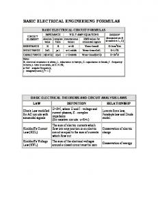
Basic Concepts In electrical engineering, we are often interested in communicating or transferring energy from one point to another. To do this requires an interconnection of electrical devices. Such interconnection is referred to as an electric circuit, and each component of the circuit is known as an element. Definition 1.0.1. An electric circuit is an interconnection of electrical elements.

1.1. Systems of Units 1.1.1. As engineers, we deal with measurable quantities. Our measurement must be communicated in standard language that virtually all professionals can understand irrespective of the country. Such an international measurement language is the International System of Units (SI). • In this system, there are six principal units from which the units of all other physical quantities can be derived. 5

6

1. BASIC CONCEPTS

Quantity Basic Unit Symbol Length meter m Mass kilogram kg Time second s Electric Current ampere A Temperature kelvin K Luminous Intensity candela cd Charge coulomb C • One great advantage of SI unit is that it uses prefixes based on the power of 10 to relate larger and smaller units to the basic unit. Multiplier 1012 109 106 103 10−2 10−3 10−6 10−9 10−12

Prefix Symbol tera T giga G mega M kilo k centi c milli m micro µ nano n pico p

Example 1.1.2. Change of units: 600, 000, 000 mA = 1.2. Circuit Variables 1.2.1. Charge: The concept of electric charge is the underlying principle for all electrical phenomena. Charge is an electrical property of the atomic particles of which matter consists, measured in coulombs (C). The charge of an electron is −1.602 × 10−19 C. • The coulomb is a large unit for charges. In 1 C of charge, there are 1/(1.602 × 10−19 ) = 6.24 × 1018 electrons. Thus realistic or laboratory values of charges are on the order of pC, nC, or µC. • A large power supply capacitor can store up to 0.5 C of charge. 1.2.2. Law of Conservation of Charge: Charge can neither be created nor destroyed, only transferred.

1.2. CIRCUIT VARIABLES

7

Definition 1.2.3. Current: The time rate of change of charge, measured in amperes (A). Mathematically, i(t) =

d q(t) dt

Note: • 1 ampere (A) = 1 coulomb/second (C/s). • The charge transferred between time t1 and t2 is obtained by Z t2 q= idt t1

1.2.4. Two types of currents: (a) A direct current (dc) is a current that remains constant with time.

(b) A time-varying current is a current that varies with time. • An alternating current (ac) is a current that varies sinusoidally with time.

8

1. BASIC CONCEPTS

• Such ac current is used in your household, to run the air conditioner, refrigerator, washing machine, and other electric appliances. 1.2.5. By convention the symbol I is used to represent such a constant current. A time-varying current is represented by the symbol i. Definition 1.2.6. Voltage (or potential difference): the energy required to move a unit charge though an element, measured in volts (V). The voltage between two points a and b in a circuit is denoted by vab and can be interpreted in two ways: (a) point a is at a potential of vab volts higher than point b, or (b) the potential at point a with respect to point b is vab . Note: • 1 volt (V) = 1 joule/coulomb = 1 newton-meter/coulomb • vab = −vba • Mathematically, dw vab = dq where w is the energy in joules (J) and q is charge in coulombs (C). +

a

vab –

b

The plus (+) and minus (-) signs at the points a and b are used to define reference direction or voltage polarity. +

a

9V –

–

a

-9 V b

+

b


9

1.2.7. Like electric current, a constant voltage is called a dc voltage and is represented by V , whereas a time-varying voltage is called an ac voltage and is represented by v. A dc voltage is commonly produced by a battery; ac voltage is produced by an electric generator. 1.2.8. Current and voltage are the two basic variables in electric circuits. The common term signal is used for an electric quantity such as a current or a voltage (or even electromagnetic wave) when it is used for conveying information. Engineers prefer to call such variables signals rather than mathematical functions of time because of their importance in communications and other disciplines. For practical purposes, we need to be able to find/calculate/measure more than the current and voltage. We all know from experience that a 100-watt bulb gives more light than a 60-watt bulb. We also know that when we pay our bills to the electric utility companies, we are paying for the electric energy consumed over a certain period of time. Thus power and energy calculations are important in circuit analysis. Definition 1.2.9. Power: time rate of expending or absorbing energy, measured in watts (W). Mathematically, the instantaneous power dw dq dw = = vi p= dt dq dt Definition 1.2.10. Sign of power • Plus sign: Power is absorbed by the element. (resistor, inductor) • Minus sign: Power is supplied by the element. (battery, generator)

Definition 1.2.11. Passive sign convention: • Passive sign convention is satisfied when the current enters through the positive terminal of an element. • If the current enters through the positive polarity of the voltage, p = vi. • If the current enters through the negative polarity of the voltage, p = −vi.

10

1. BASIC CONCEPTS

i

i +

+

v

v

–

–

p = +vi

p = –vi

3A

3A

+

–

4V

4V

–

+

3A

3A

+

–

4V

4V

–

+

Example 1.2.12. Light bulb or battery


11

1.2.13. Law of Conservation of Energy: Energy can neither be created nor destroyed, only transferred. • For this reason, the algebraic sum of power in a circuit, at any instant of time, must be zero. • The total power supplied to the circuit must balance the total power absorbed. Example 1.2.14. The circuit below has five elements. If p1 = −205 W, p2 = 60 W, p4 = 45 W, p5 = 30 W, calculate the power p3 received or delivered by element 3.

1.2.15. Energy: the energy absorbed or supplied by an element from time 0 to t is Z t Z t w= p dt = vi dt. 0

0

• Integration suggests finding area under the curve. • Need to be careful with negative area. Example 1.2.16. Electricity bills: The electric power utility companies measure energy in kilowatt-hours (kWh), where 1 kWh = 3600 kJ.

12

1. BASIC CONCEPTS

1.3. Circuit Elements Definition 1.3.1. There are 2 types of elements found in electrical circuits. 1) Active elements (is capable of generating energy), e.g., generators, batteries, and operational amplifiers (Op-amp). 2) Passive element, e.g., resistors, capacitors and inductors. Definition 1.3.2. The most important active elements are voltage and current sources: (a) Voltage source provides the circuit with a specified voltage (e.g. a 1.5V battery) (b) Current source provides the circuit with a specified current (e.g. a 1A current source). Definition 1.3.3. In addition, we may characterize the voltage or current sources as: 1) Independent source: An active element that provides a specified voltage or current that is completely independent of other circuit elements.

v

+ V –

DC

i

1.3. CIRCUIT ELEMENTS

13

2) Dependent source: An active element in which the source quantity is controlled by another voltage or current.

v

+ –

i

1.3.4. The key idea to keep in mind is that a voltage source comes with polarities (+ -) in its symbol, while a current source comes with an arrow, irrespective of what it depends on. Example 1.3.5. Current-controlled voltage source A

B i

+ 5V –

C

+ –

10i

Example 1.3.6. Draw the general form of a voltage-controlled current cource.

14

1. BASIC CONCEPTS

1.3.7. Remarks: • Dependent sources are useful in modeling elements such as transistors, operational amplifiers and integrated circuits. • Ideal sources – An ideal voltage source (dependent or independent) will produce any current required to ensure that the terminal voltage is as stated. – An ideal current source will produce the necessary voltage to ensure the stated current flow. – Thus an ideal source could in theory supply an infinite amount of energy. • Not only do sources supply power to a circuit, they can absorb power from a circuit too. • For a voltage source, we know the voltage but not the current supplied or drawn by it. By the same token, we know the current supplied by a current source but not the voltage across it.

CHAPTER 2

Basic Laws Here we explore two fundamental laws that govern electric circuits (Ohm’s law and Kirchhoff’s laws) and discuss some techniques commonly applied in circuit design and analysis. 2.1. Ohm’s Law Ohm’s law shows a relationship between voltage and current of a resistive element such as conducting wire or light bulb.

2.1.1. Ohm’s Law: The voltage v across a resistor is directly proportional to the current i flowing through the resistor. v = iR, where R = resistance of the resistor, denoting its ability to resist the flow of electric current. The resistance is measured in ohms (Ω). • To apply Ohm’s law, the direction of current i and the polarity of voltage v must conform with the passive sign convention. This implies that current flows from a higher potential to a lower potential 15

16

2. BASIC LAWS

in order for v = iR. If current flows from a lower potential to a higher potential, v = −iR.

i

l

Material with Cross-sectional resistivity r area A

+ v –

R

2.1.2. The resistance R of a cylindrical conductor of cross-sectional area A, length L, and conductivity σ is given by L R= . σA Alternatively, L R=ρ A where ρ is known as the resistivity of the material in ohm-meters. Good conductors, such as copper and aluminum, have low resistivities, while insulators, such as mica and paper, have high resistivities. 2.1.3. Remarks: (a) R = v/i (b) Conductance : 1 i = R v 1 The unit of G is the mho (f) or siemens2 (S) G=

1Yes, this is NOT a typo! It was derived from spelling ohm backwards. 2In English, the term siemens is used both for the singular and plural.

2.1. OHM’S LAW

17

(c) The two extreme possible values of R. (i) When R = 0, we have a short circuit and v = iR = 0 showing that v = 0 for any i.

+

i

v=0 R=0 –

(ii) When R = ∞, we have an open circuit and v =0 i = lim R→∞ R indicating that i = 0 for any v.

+ v

i=0 R=∞

–

2.1.4. A resistor is either fixed or variable. Most resistors are of the fixed type, meaning their resistance remains constant.

18

2. BASIC LAWS

A common variable resistor is known as a potentiometer or pot for short

2.1.5. Not all resistors obey Ohms law. A resistor that obeys Ohms law is known as a linear resistor. • A nonlinear resistor does not obey Ohms law.

• Examples of devices with nonlinear resistance are the lightbulb and the diode. • Although all practical resistors may exhibit nonlinear behavior under certain conditions, we will assume in this class that all elements actually designated as resistors are linear.

2.1. OHM’S LAW

19

2.1.6. Using Ohm’s law, the power p dissipated by a resistor R is v2 p = vi = i2 R = . R Example 2.1.7. In the circuit below, calculate the current i, and the power p.

i 30 V

DC

5 kΩ

+ v –

Definition 2.1.8. The power rating is the maximum allowable power dissipation in the resistor. Exceeding this power rating leads to overheating and can cause the resistor to burn up. Example 2.1.9. Determine the minimum resistor size that can be connected to a 1.5V battery without exceeding the resistor’s 14 -W power rating.

more complicated examples, including the one shown in Figure 2.1.

2.1 T E R M I N O L O G Y Lumped circuit elements are the fundamental building blocks of electronic cir2. BASIC LAWS cuits. Virtually all of our analyses will be conducted on circuits containing two-terminal elements; multi-terminal elements will be modeled using combinations of two-terminal elements. We have already seen several two-terminal Node, Branches and Loops elements such 2.2. as resistors, voltage sources, and current sources. Electronic access to an element is made through its terminals. Definition 2.2.1. Since the elements of an electric circuit can be interAn electronic circuit is constructed by connecting together a collection of connected in ways, we need to understand some basic concept of separateseveral elements at their terminals, as shown in Figure 2.2. The junction points networkattopology. which the terminals of two or more elements are connected are referred to as the nodes of=a circuit. Similarly, the connections between the nodes are referred • Network interconnection of elements or devices to as the edges or branches of a circuit. Note that each element in Figure 2.2 • Circuit = a branch. network closedandpaths forms a single Thuswith an element a branch are the same for circuits comprising only two-terminal circuit a loops are defined to besuch as a Definition 2.2.2. Branch: A elements. branch Finally, represents single element closed paths through a circuit along its branches. voltage source or nodes, a resistor. Aand branch represents Several branches, loops are identified inany Figuretwo-terminal 2.2. In the circuitelement. in Figure 2.2, there are 10 branches (and thus, 10 elements) and 6 nodes. Definition 2.2.3. Node: A node is the “point” of connection between As another example, a is a node in the circuit depicted in Figure 2.1 at two or more branches. which three branches meet. Similarly, b is a node at which two branches meet. ab and bc are of branches in thein circuit. The circuit has five branches • It is usuallyexamples indicated by a dot a circuit. nodes. • Ifand a four short circuit (a connecting wire) connects two nodes, the two Since we assume that the interconnections between the elements in a circuit nodes constitute a single node. are perfect (i.e., the wires are ideal), then it is not necessary for a set of elements to be joined at aAsingle in space for their interconnection to beA closed Definition 2.2.4.together Loop: looppoint is any closed path in a circuit. considered a single node. An example of this is shown in Figure 2.3. While path is formed by starting at aare node, passing through a set ofdoes nodes and the four elements in the figure connected together, their connection returning theat starting node without passing throughconnection. any node more notto occur a single point in space. Rather, it is a distributed 20

than once. Nodes Loop

Elements

E 2.2 An arbitrary circuit.

Branch

Definition 2.2.5. Series: Two or more elements are in series if they are cascaded or connected sequentially and consequently carry the same current. Definition 2.2.6. Parallel: Two or more elements are in parallel if they are connected to the same two nodes and consequently have the same voltage across them. 2.2.7. Elements may be connected in a way that they are neither in series nor in parallel.

2.2. NODE, BRANCHES AND LOOPS

21

Example 2.2.8. How many branches and nodes does the circuit in the following figure have? Identify the elements that are in series and in parallel. 5Ω

1Ω

2Ω

DC

10 V

4Ω

2.2.9. A loop is said to be independent if it contains2.2 a branch which is Kirchhoff’s Laws not in any other loop. Independent loops or paths result in independent sets of equations. A network with b branches, n nodes, and ` independent loops will satisfy the fundamental theorem of network topology: B

Elements

b = ` + n − 1.

B

C

aA circuit Care

Definition 2.2.10. The primary signals within its currents A and voltages, which we denote by the symbols i and Dv, respectively. We Distributed node D define a branch current as the current along a branch of the circuit, and Ideal wires a branch voltage as the potential difference measured across a branch.

CHAPTER T

F I G U R E 2.3 interconnectio elements that at a single nod

i Branch current

v

+

Branch voltage

Nonetheless, because the interconnections are perfect, the connection can be considered to be a single node, as indicated in the figure. The primary signals within a circuit are its currents and voltages, which we denote by the symbols i and v, respectively. We define a branch current as the current along a branch of the circuit (see Figure 2.4), and a branch voltage as the potential difference measured across a branch. Since elements and branches are the same for circuits formed of two-terminal elements, the branch voltages and currents are the same as the corresponding terminal variables for the elements forming the branches. Recall, as defined in Chapter 1, the terminal variables for an element are the voltage across and the current through the element. As an example, i4 is a branch current that flows through branch bc in the circuit in Figure 2.1. Similarly, v4 is the branch voltage for the branch bc.

F I G U R E 2.4 deﬁnitions illu a circuit.

22

2. BASIC LAWS

2.3. Kirchhoff ’s Laws Ohm’s law coupled with Kirchhoff’s two laws gives a sufficient, powerful set of tools for analyzing a large variety of electric circuits. 2.3.1. Kirchhoff ’s current law (KCL): the algebraic sum of currents departing a node (or a closed boundary) is zero. Mathematically, X in = 0 n

KCL is based on the law of conservation of charge. An alternative form of KCL is Sum of currents (or charges) drawn as entering a node = Sum of the currents (charges) drawn as leaving the node.

i5

i1

i4 i2 i3

Note that KCL also applies to a closed boundary. This may be regarded as a generalized case, because a node may be regarded as a closed surface shrunk to a point. In two dimensions, a closed boundary is the same as a closed path. The total current entering the closed surface is equal to the total current leaving the surface. Closed boundary

2.3. KIRCHHOFF’S LAWS

23

Example 2.3.2. A simple application of KCL is combining current sources in parallel. IT a I1 b

I2

I3

(a) IT a IT = I 1 – I2 + I 3 b

(b)

A Kirchhoff ’s voltage law (KVL): the algebraic sum of all voltages around a closed path (or loop) is zero. Mathematically, M X

vm = 0

m=1

KVL is based on the law of conservation of energy. An alternative form of KVL is Sum of voltage drops = Sum of voltage rises. +

v2 –

+

v1

v3 –

v4

– v5 +

24

2. BASIC LAWS

Example 2.3.3. When voltage sources are connected in series, KVL can be applied to obtain the total voltage. a

+ V1 Vab

V2

a

Vab

V3 b

–

+

b

VS = V1 + V2 – V3

–

Example 2.3.4. Find v1 and v2 in the following circuit. 4Ω + v1 – 10 V

8V +

v2 – 2Ω

2.4. SERIES RESISTORS AND VOLTAGE DIVISION

25

2.4. Series Resistors and Voltage Division 2.4.1. When two resistors R1 and R2 ohms are connected in series, they can be replaced by an equivalent resistor Req where Req = R1 + R2 . In particular, the two resistors in series shown in the following circuit i

R1

R2

+ v1 –

+ v2 –

a

v

b

can be replaced by an equivalent resistor Req where Req = R1 +R2 as shown below.

i

a

Req + v –

v

b The two circuits above are equivalent in the sense that they exhibit the same voltage-current relationships at the terminals a-b. Voltage Divider: If R1 and R2 are connected in series with a voltage source v volts, the voltage drops across R1 and R2 are R1 R2 v and v2 = v v1 = R1 + R2 R1 + R2

26

2. BASIC LAWS

Note: The source voltage v is divided among the resistors in direct proportion to their resistances. 2.4.2. In general, for N resistors whose values are R1 , R2 , . . . , RN ohms connected in series, they can be replaced by an equivalent resistor Req where N X Req = R1 + R2 + · · · + RN = Rj j=1

If a circuit has N resistors in series with a voltage source v, the jth resistor Rj has a voltage drop of Rj v vj = R1 + R2 + · · · + RN 2.5. Parallel Resistors and Current Division

When two resistors R1 and R2 ohms are connected in parallel, they can be replaced by an equivalent resistor Req where 1 1 1 = + Req R1 R2 or R1 R2 Req = R1 kR2 = R1 + R2

i

Node a i1

v

i2 R1

R2

Node b Current Divider: If R1 and R2 are connected in parallel with a current source i, the current passing through R1 and R2 are R2 R1 i1 = i and i2 = i R1 + R2 R1 + R2 Note: The source current i is divided among the resistors in inverse proportion to their resistances.

2.5. PARALLEL RESISTORS AND CURRENT DIVISION

27

Example 2.5.1.

Example 2.5.2. 6k3 = Example 2.5.3. (a)k(na) = Example 2.5.4. (ma)k(na) = In general, for N resistors connected in parallel, the equivalent resistor Req = R1 kR2 k · · · kRN is 1 1 1 1 = + + ··· + Req R1 R2 RN Example 2.5.5. Find Req for the following circuit. 4Ω

1Ω 2Ω

Req

5Ω 8Ω

6Ω

3Ω

Example 2.5.6. Find the equivalent resistance of the following circuit.

28

2. BASIC LAWS

i

4Ω

i0

a

6Ω

12 V

+ v0 –

3Ω

b

Example 2.5.7. Find io , vo , po (power dissipated in the 3Ω resistor).

Example 2.5.8. Three light bulbs are connected to a 9V battery as shown below. Calculate: (a) the total current supplied by the battery, (b) the current through each bulb, (c) the resistance of each bulb. I

9V

15 W 20 W

9V 10 W

I1 I2

+ V2 –

R2

+ V3 –

R3

+ V1 –

R1

2.7. MEASURING DEVICES

29

2.6. Practical Voltage and Current Sources An ideal voltage source is assumed to supply a constant voltage. This implies that it can supply very large current even when the load resistance is very small. However, a practical voltage source can supply only a finite amount of current. To reflect this limitation, we model a practical voltage source as an ideal voltage source connected in series with an internal resistance rs , as follows:

Similarly, a practical current source can be modeled as an ideal current source connected in parallel with an internal resistance rs . 2.7. Measuring Devices Ohmmeter: measures the resistance of the element. Important rule: Measure the resistance only when the element is disconnected from circuits. Ammeter: connected in series with an element to measure current flowing through that element. Since an ideal ammeter should not restrict the flow of current, (i.e., cause a voltage drop), an ideal ammeter has zero internal resistance. Voltmeter:connected in parallel with an element to measure voltage across that element. Since an ideal voltmeter should not draw current away from the element, an ideal voltmeter has infinite internal resistance.