Matrix Element Randomness, Entanglement, and Quantum Chaos Yaakov S. Weinstein1, ∗ and C. Stephen Hellberg1, †
arXiv:quant-ph/0405053v1 11 May 2004
1
Center for Computational Materials Science, Naval Research Laboratory, Washington, DC 20375
We demonstrate the connection between an operator’s matrix element distribution and entangling power via numerical simulations of random, pseudo-random, and quantum chaotic operators. Creating operators with a random distribution of matrix elements is more difficult than creating operators that reproduce other statistical properties of random matrices. Thus, operators that fulfill many random matrix statistical properties may not generate states of high multi-partite entanglement. To quantify the randomness of various statistical distributions and, by extension, entangling power, we use properties of interpolating ensembles that transition between integrable and random matrix ensembles. PACS numbers: 03.67.Mn 05.45.Mt 03.67.Lx
Random matrices have long been used as statistical models for a host of complex systems in areas of physics ranging from quantum dots to field theory [1]. Originally introduced by Wigner to predict the energy level spectrum of heavy atomic nuclei [2], random matrices were later applied to characterize quantum chaotic systems [3, 4, 5]. More recently, random matrices have been found essential in various protocols of quantum computation and communication including quantum state superdense coding [6], remote state preparation [8], data hiding schemes [7], and entangled state production [9]. Given the similarities between quantum chaotic operators and random matrices, and the aptitude of random matrices for producing entangled states, several authors have proposed entanglement production as an indicator of quantum chaos [10, 11, 12]. While there has been some debate [13], substantial numerical evidence suggests that quantum systems with underlying chaotic classical dynamics produce entanglement at a faster rate than systems with underlying regular dynamics. In this work we explore the distribution of unitary operator matrix element amplitudes, a statistical criterion of random matrices [14]. We show that the matrix elements are key to entanglement production. Furthermore, we demonstrate that, in creating an operator, it is more difficult to reproduce the statistical properties of the elements of random matrices than other random matrix properties. Evidence is provided from matrix ensembles that transition between integrable and random matrices, known as the interpolating ensembles, and pseudo-random matrices. For these classes of matrices nearest neighbor eigenvalue spacing and eigenvector element distributions converge to that of random matrices more quickly than the matrix element distribution. The entanglement production of these operators is correspondingly slower in converging to that of random matrix
production. We also use interpolating ensembles properties to quantify the randomness of a given statistical distribution and, by extension, entanglement production. Finally, we discuss the role of the matrix element distribution in the entanglement production of quantum chaotic operators: why the entanglement produced increases with time, and how the entanglement production differs from non-chaotic operators. The circular ensembles of random unitary matrices were introduced by Dyson [15] as alternatives to the Gaussian ensembles of random Hermitian matrices [2, 16]. As with the Gaussian ensembles, the circular ensembles play a central role in modeling complex quantum systems. Unlike the Gaussian ensembles, however, elements of the unitaries are not independent random variables [17] and are thus more difficult to generate. Nevertheless, matrices of the circular unitary ensemble (CUE), the space of all unitary matrices, can be generated by taking the eigenvectors of a Hermitian matrix belonging to the Gaussian unitary ensemble (GUE), multiplying each by a random phase, and using the resulting vectors as the matrix columns [14]. The squared modulus or amplitude of the CUE matrix elements follow a distribution equal to that of GUE eigenvector element amplitudes. Let clk denote the kth component of the lth GUE eigenvector. The distribution of amplitudes η = |clk |2 in the limit of infinite Hilbert space dimension, N → ∞, after rescaling to a unit mean is PGUE (y) = e−y , where y = N η [4]. Since η is unchanged when multiplied by a phase, the distribution, PCUE (x), of the rescaled amplitude of CUE matrix elements x, is equal to PGUE (y). CUE matrices can also be generated based on the Hurwitz parameterization using elementary unitary transformations, E (i,j) (φ, ψ, χ) with non-zero elements (i,j)
Ekk ∗ To whom correspondence should be addressed; Electronic address:
[email protected] † Electronic address:
[email protected]
(i,j) Eii (i,j)
Eji
= 1,
k = 1, ..., N,
k 6= i, j
= eiψ cos φ,
(i,j) Eij
= −e−iχ sin φ,
Ejj
(i,j)
= eiχ sin φ = e−iψ cos φ
(1)
2 to construct N − 1 composite rotations
1
(2)
0 ≤ χs ≤ 2π,
0 ≤ α ≤ 2π,
(3)
and φrs = sin−1 (ξrs 1/(2r+2) ), with ξrs drawn uniformly (i,j) from 0 to 1 [17]. Note that the 2 × 2 block Em,n with m, n = i, j and r = 0 is a random SU(2) rotation with respect to the Haar measure. An advantage of the above method is that it allows for a one-parameter interpolation between diagonal matrices with uniform, independently distributed elements and CUE [18]. This is done by drawing the above parameters from constricted intervals 0 ≤ ψrs ≤ 2πδ,
0 ≤ χs ≤ 2πδ,
0 ≤ α ≤ 2πδ, (4)
1/(2r+2)
and setting φrs = sin−1 (δξij ) with ξrs now drawn from 0 to δ. The whole is multiplied by a diagonal matrix of random phases drawn uniformly from 0 to 2π. The parameter δ ranges from 0 to 1 and provides a smooth transition between the diagonal circular Poisson ensemble (CPE) and CUE for nearest neighbor eigenvalue and eigenvector statistics [18]. The interpolating ensembles matrix element amplitude distribution, however, does not transition smoothly with δ. Rather, the matrix element randomness lags behind that of the other criteria such that even large δ induces matrix element distributions noticeably different from PCUE (x) as in figure 1. A practical measure of multi-partite entanglement is the average bipartite entanglement between each qubit and the rest of the system [19, 20], 2X T r[ρ2j ], n j=1 n
Q=2−
(5)
where ρj is the reduced density matrix of qubit j. An operators’ lack of matrix element randomness causes the distribution of Q, for computational basis states evolved under one iteration of the operator, to diverge sharply from PCUE (Q), the distribution expected for states evolved by CUE matrices. For the interpolating ensembles a high value of δ, such as δ = .98, yields eigenvalue and eigenvector distributions extremely close to CUE. P (Q), however, is still far from PCUE (Q) due
0.6
10
eigenvector elements
0.4 0.2
1
2
0
3
−6
−4 −2 log (y)
0
2
10
entanglement
matrix elements
P(Q)
0.8
and, finally, UCUE = eiα E1 E2 . . . EN −1 . Angles ψ, χ, and α are drawn uniformly from the intervals 0 ≤ ψrs ≤ 2π,
0.6
s
P[log10(x)]
(φ0,N −1 , ψ0,N −1 , χN −1 )
0.4
0
E (2,3) (φN −3,N −1 , ψN −3,N −1 , 0) ×
... E
0.6
0.2
EN −1 = E (1,2) (φN −2,N −1 , ψN −2,N −1 , 0) × (N −1,N )
P[log (y)]
E2 = E (N −2,N −1) (φ12 , ψ12 , 0)E (N −1,N ) (φ02 , ψ02 , χ2 ) ...
P(s)
E1 = E (N −1,N ) (φ01 , ψ01 , χ1 )
0.8
eigenvalue spacings
0.8
0.4 0.2 0
−6
−4 −2 log10(x)
0
2
0.9
0.95 Q
1
FIG. 1: (Color online) Distributions of nearest neighbor eigenvalue spacings (upper-left) and eigenvector element amplitudes (upper-right) for matrices of the interpolating ensembles with δ = .1 (dashed), .5 (dotted) and .9 (chained). The matrix element plot (lower-left) also includes the distribution for δ = .98 (light solid line). For this δ the eigenvalue and eigenvector distributions are indistinguishable from random (solid line), but the matrix element distribution converges much more slowly. This is manifest in the entanglement generated by operating with 100 8-qubit matrices on all computational basis states, shown on the lower right for δ = .9 (o), and .98 (diamonds).
to lack of randomness in the matrix elements as seen in figure 1. The δ characterized distributions of the interpolating ensembles provide a quantifiable randomness measure for not fully random distributions. Such a measure provides objectivity in reporting the distance a given distribution is from the random one and allows the randomness of different statistical criteria to be compared. Not all nonrandom statistics will follow one of these intermediate distributions, but we find them useful nevertheless. The randomness of an operator’s matrix element distribution can be quantified by fitting it with an interpolating ensemble eigenvector distribution. Since an operators’ matrix element distribution determines the amount of entanglement generated, reporting δ of the eigenvector distribution best fit provides a measure of entangling power. An operator or class of operators whose matrix element distribution conforms to a higher δ-eigenvector distribution produces, on average, more entanglement. To generate a semi-random state with a given amount of entanglement, a quantum computer programmer can apply an operator with the desired matrix distribution δ. We note that the interpolating ensemble matrix elements themselves are not well estimated by the δ-eigenvalue distributions. This most likely stems from constrictions of the Euler angles, Eq. (4), which also leads to a nonsmooth entanglement distribution. To further explore the relationship between matrix element amplitude distributions, entanglement, and other
3
i(π/4)
n−1
σj ⊗σj+1
z z j=1 , where σzj is the z-direction Pauli e spin operator. The random rotations are different for each qubit and each iteration, but the coupling constant is always π/4 to maximize entanglement. After the m iterations, a final set of random rotations is applied.
As m increases, the statistical properties of the pseudorandom operators converge to those of random operators [21]. However, as seen in figure 2, these properties do not converge at the same rate. For n = 8, m = 2 the eigenvalue spacing distribution is well approximated by the δ = .8 interpolating ensemble eigenvalue spacing distribution, the eigenvectors by the δ = .92 eigenvector element distribution, and the matrix elements by the δ = .7 eigenvector element distribution. Applying 100 m = 2 maps to all computational basis states gives an average entanglement hQi of .7004 compared to .9883 for CUE matrices. For m = 4 the eigenvalues are approximated by δ = .9, while the eigenvectors are indistinguishable from the random distribution. The matrix elements are approximated by a δ of .78 and hQi = .8416. Operators of higher m lead to eigenvalue and eigenvector distributions that are practically random. The matrix elements, however, lag behind with δ = .88 and hQi = .9339 for m = 8 and δ = .98 and hQi = .9790 for m = 16. The above examples illustrate the difficulty in generating operators with a random distribution of matrix elements. In both cases increasing one parameter, δ for the interpolating ensembles and m for the pseudo-random operators, causes a convergence to CUE statistics. The convergence is relatively quick for eigenvalue and eigenvector distributions but much slower for the matrix element distribution. The correspondingly slow convergence of entanglement production to PCUE (Q) is evidence of the connection between the matrix element distribution and entanglement generation. Quantum chaotic operators are known for their ability to produce entanglement. Numerical simulations of two coupled subsystems demonstrate the greater entanglement generation of chaotic versus regular quantum dynamics [10, 11, 12] and analytical results have been obtained through various methods [13, 24, 25]. Here, we are interested in a quantum chaotic operator’s ability to produce entanglement on a quantum computer. Applying a chaotic operator once will not, in general, produce entan-
1
P[log (y)]
0.6
0.6
0.4 0.2 0 0
1
0.4 0.2 0
2 s
0.6
matrix elements
−2
−1 0 log10(y)
1
entanglement
P(Q)
0.8
eigenvector elements
10
P(s)
0.8
eigenvalue spacings
0.8
P[log10(x)]
statistical measures of randomness, we turn to pseudorandom operators [21, 22, 23]. Despite being efficiently implementable on a quantum computer, pseudo-random operators have been shown to reproduce statistical properties of random operators. The pseudo-random operator algorithm is to apply m iterations of the n qubit gate: random SU(2) rotation to each qubit, then evolve the system via all nearest neighbor couplings [21]. A random SU(2) rotation with respect to the Haar measure is described by equations Eqs. (1) and (3). The nearestPneighbor coupling operator we use is Unnc =
0.4 0.2 0
−2
−1 0 log10(x)
1
0.9
0.95 Q
1
FIG. 2: (Color online) Distribution of nearest neighbor eigenvalue spacings (top left), eigenvector elements (top right), matrix elements (bottom left), and Q (bottom right) for 8-qubit pseudo-random maps of m = 2 (plus), 4 (x), 8 (square), and 16 (o). The eigenvalue and eigenvector distributions converge to that of random matrices (solid lines) more quickly than the matrix element distribution. The eigenvalue spacing for m = 2 and 4 are fitted by the δ = .8 (chained line) and .94 (dashed line) eigenvalue distributions. The m = 2 eigenvector distribution is approximated by δ = .92 (chained line). The distribution of matrix elements for the m = 2, 4, 8 and 16 pseudo-random operators can be approximated by δ = .7 (chained line), .78 (dashed line), .88 (solid line), and .98 (dotted line) respectively. The low entanglement production is a direct outgrowth of the matrix element randomness lag. To approach PCU E (Q) requires m ≃ 40 [21].
glement on par with random operators [9, 26]. After a number of iterations, however, the average entanglement of initial computational basis states hQ(t)i, where t is the number of operator iterations, can approach that of random operators. We show how this is attributable to the matrix element distribution. First, we note that an increase in hQ(t)i with time cannot be due to eigenvector or eigenvalue statistics. The eigenvectors of an operator are unchanged as a function of t and the eigenvalues become uncorrelated. The randomness of the matrix elements of chaotic operators, however, increases with t. To demonstrate this assertion we revisit entanglement production of the quantum baker’s map [9] and explore other quantized chaotic maps. Initial computational basis states evolved under the quantum baker’s map attain Q values close to the random matrix average only at large t [9]. Figure 3C shows that this is due to the map’s matrix element distribution. The baker’s map matrix elements do not at all resemble PCUE (x), however, for t = 100 the distribution is well approximated by the δ = .9 interpolating ensemble eigenvalue distribution. For the n = 8 baker’s map hQ(1)i is only .3080, while hQ(100)i is .9597. More iterations lead to increased matrix element randomness which causes greater entanglement generation.
4 Other examples of quantized chaotic maps are the quantum sawtooth map [27, 28], Usaw = 2 2 e−iπ/4 √ eikπm /N eiπ(n−m) /N , and the quantum Harper N
0.95 0.9 0.85
Q
map [29], UH = eiN γ cos(2πq/N ) eiN γ cos(2πp/N ) . All elements of the chaotic, k = 1.5, and regular, k = −1.5, sawtooth maps have equal amplitude. Operating on any computational basis state yields a state of Q = 1. For the chaotic sawtooth the matrix element randomness increases with t, such that at t = 50 the matrix element distribution is practically PCUE (x) and hQ(50)i = .98826. For the regular sawtooth the entanglement oscillates wildly as seen in figure 3. This stems from the lack of an asymptotic randomness for the matrix elements.
1
0.8 0.75
0.8 P[log (x)]
0.8
0.8
0.6
0.6
0.6
0.4
0.4
0.4
0.2
0.2
10
0.7 0.65
0
0.6
A −3
−2
−1
10
0
1
0
0.2
B −3
−2
−1
20
0
30
1
0
C −3
−2
40
−1
0
1
50
t
The matrix elements for the chaotic Harper, γ = 1, deviate only slightly from PCUE (x), and, thus, hQ(1)i = .9814. For t = 50 there is the expected increase in matrix element randomness and hQ(50)i = .9882. The regular Harper map, γ = .1, matrix element distribution and average entanglement also approach asymptotic limits as t increases. However, these limits fall short of the random matrix statistics. The matrix element distribution is well fit by the δ = .9 interpolating ensemble eigenvector element distribution and the average entanglement hQ(t → ∞)i ≃ .95. We note that the matrix elements of the 100 times iterated baker’s map and the m = 8 pseudo-random operators also follow the δ = .9 distribution. Thus, hQ(50)i of the regular harper is very close to hQi of these operators.
FIG. 3: (Color online) Average entanglement, Q, over all 8qubit initial computational basis states as a function of time for quantum sawtooth maps, k = 1.5 (chained line) and k = −1.5 (dotted line) and Harper maps, γ = 1 (solid line) and γ = .1 (dashed line), compared to the random matrix average (horizontal dashed line). The chaotic maps quickly approach the random matrix average while the regular maps do not. The insets show matrix element distributions for the regular (light) and chaotic (dark) sawtooth maps at t = 50 (A), the regular (light) and chaotic (dark) Harper maps at t = 50 (B), and t = 1 (light) and 100 (dark) of the baker’s map (C). The matrix elements for the t = 50 regular Harper map is well approximated by the δ = .94 eigenvalue distribution.
In conclusion, we have explored connections between a system’s matrix element distribution and entanglement production. The interpolating ensembles demonstrate the difficulty in creating operators with randomly distributed matrix elements and their statistical properties provide a useful measure of randomness. This measure is used to compare and contrast the randomness of statistical distributions from pseudo-random and chaotic operators. The connection to matrix element randomness provides a random matrix basis for increased entanglement production of chaotic systems as a function of time and the greater entanglement production for chaotic versus non-chaotic systems. Though this need not always be the case, operators with similar matrix element distributions appear, on average, to produce states with a similar amount of entanglement.
[1] See T. Guhr, A. M¨ uller-Groeling, H.A. Weidenm¨ uller, Phys. Rep., 299, 189, (1998) for a comprehensive review. [2] E.P. Wigner, Ann. Math. 62, 548 (1955); 65, 203 (1957). [3] O. Bohigas, M.J. Giannoni, C. Schmit, Phys. Rev. Lett., 52, 1, (1984). [4] F. Haake, K. Zyczkowski, Phys. Rev. A, 42, 1013, (1990). [5] F. Haake, Quantum Signatures of Chaos, (Springer, New York, 1992). [6] A. Harrow, P. Hayden, D. Leung, Phys. Rev. Lett. 92, 187901 (2004). [7] P. Hayden, D. Leung, P. Shor, A. Winter, quant-ph/0307104. [8] C.H. Bennett, P. Hayden, D. Leung, P. Shor, A. Winter, quant-ph/0307100. [9] A. Scott, C. Caves, J. Phys. A, 36, 9553, (2003). [10] A. Lakshminarayan, Phys. Rev. E, 64, 036207, (2001); J.N. Bandyopadhyay, A. Lakshminarayan, Phys. Rev. Lett., 89, 060402, (2002). [11] K. Furuya, M.C. Nemes, G.Q. Pellegrino, Phys. Rev. Lett., 80, 5524, (1998). [12] P.A. Miller, S. Sarkar, Phys. Rev. E, 60, 1542 (1999). [13] A. Tanaka, H. Fujisaki, T. Miyadera, Phys. Rev. E, 66, 045201(R), (2002). H. Fujisaki, T. Miyadera, A. Tanaka, Phys. Rev. E, 67, 066201, (2003). [14] M. Pozniak, K. Zyczkowski, M. Kus, J. Phys. A, 31, 1059, (1998). [15] F.J. Dyson, J. Math. Phys. 3, 140, (1962); [16] M.L. Mehta, Random Matrices, (Academic Press, New York, 1991).
The authors thank K. Zyczkowski for clarifying interpolating ensemble generation. The authors acknowledge support from the DARPA QuIST (MIPR 02 N699-00) program. YSW acknowledges the support of the National Research Council Research Associateship Program through the Naval Research Laboratory. Computations were performed at the ASC DoD Major Shared Resource Center.
5 [17] K. Zyczkowski, M. Kus, J. Phys. A, 27, 4235, (1994). [18] K. Zyczkowski, M. Kus, Phys. Rev. E, 53, 319, (1996). [19] D.A. Meyer, N.R. Wallach, J. Math. Phys., 43, 4273, (2002). [20] G.K. Brennen, Quant. Inf. Comp., 3, 619, (2003). [21] J. Emerson, Y.S. Weinstein, M. Saraceno, S. Lloyd, D.G. Cory, Science, 302, 2098, (2003). [22] Y.S. Weinstein, C.S. Hellberg, quant-ph/0402157. [23] Y.S. Weinstein, C.S. Hellberg, Phys. Rev. A, to be published, quant-ph/0401040. [24] J.N. Bandyopadhyay, A. Lakshminarayan, Phys. Rev. E,
69, 016201, (2004). [25] Ph. Jacquod, Phys. Rev. Lett., 92, 150403, (2004). [26] X. Wang, S. Ghose, B.C. Sanders, B. Hu, quant-ph/0312047. [27] A. Lakshminarayan, N.L. Balzs, Chaos Soliton Fract., 5, 1169, (1995). [28] G. Benenti, G. Casati, S. Montangero, D.L. Shepelyansky, Phys. Rev. Lett., 87, 227901, (2001). [29] P. Leboeuf, J. Kurchan, M. Feingold, D.P. Arovas, Phys. Rev. Lett., 65, 3076, (1990).