Ocean Sci., 5, 649–660, 2009 www.ocean-sci.net/5/649/2009/ © Author(s) 2009. This work is distributed under the Creative Commons Attribution 3.0 License.
Ocean Science
Mediterranean Forecasting System: forecast and analysis assessment through skill scores M. Tonani1 , N. Pinardi2 , C. Fratianni1 , J. Pistoia1 , S. Dobricic3 , S. Pensieri4 , M. de Alfonso5 , and K. Nittis6 1 Istituto
Nazionale di Geofisica e Vulcanologia, Bologna, Italy of Bologna, Corso di Scienze Ambientali, Ravenna, Italy 3 Centro euro-Mediterraneo per i Cambiamenti Climatici, Bologna, Italy 4 Consiglio Nazionale delle Ricerche-ISSIA, Genova, Italy 5 Puertos del Estado, Madrid, Spain 6 Hellenic Centre for Marine Research, Athens, Greece 2 University
Received: 8 January 2007 – Published in Ocean Sci. Discuss.: 22 February 2007 Revised: 10 November 2009 – Accepted: 12 November 2009 – Published: 7 December 2009
Abstract. This paper describes the first evaluation of the quality of the forecast and analyses produced at the basin scale by the Mediterranean ocean Forecasting System (MFS) (http://gnoo.bo.ingv.it/mfs). The system produces short-term ocean forecasts for the following ten days. Analyses are produced weekly using a daily assimilation cycle. The analyses are compared with independent data from buoys, where available, and with the assimilated data before the data are inserted. In this work we have considered 53 ten days forecasts produced from 16 August 2005 to 15 August 2006. The forecast skill is evaluated by means of root mean square error (rmse) differences, bias and anomaly correlations at different depths for temperature and salinity, computing differences between forecast and analysis, analysis and persistence and forecast and persistence. The Skill Score (SS) is defined as the ratio of the rmse of the difference between analysis and forecast and the rmse of the difference between analysis and persistence. The SS shows that at 5 and 30 m the forecast is always better than the persistence, but at 300 m it can be worse than persistence for the first days of the forecast. This result may be related to flow adjustments introduced by the data assimilation scheme. The monthly variability of SS shows that when the system variability is high, the values of SS are higher, therefore the forecast has higher skill than persistence. We give evidence that the error growth in the surface layers is controlled by the atmospheric forcing inaccuracies, while
Correspondence to: M. Tonani (
[email protected])
at depth the forecast error can be interpreted as due to the data insertion procedure. The data, both in situ and satellite, are not homogeneously distributed in the basin; therefore, the quality of the analyses may be different in different areas of the basin.
1
Introduction
The aim of this study is to evaluate the accuracy of the forecast produced at the basin scale by the Mediterranean ocean Forecasting System (MFS), developed during MFSPilot Projetc,MFSPP (Pinardi et al., 2003) and MFS-Toward Environmental Predictions, MFSTEP projects. The existence of a forecasting system is important since the information delivered add some knowledge to the future event of interest. For an operational forecasting system there is therefore a need to do a validation of the products everywhere and for every single forecast day (Jolliffe and Stephenson, 2003). The forecast could be used for scientific or operational application if there is an information of the accuracy of the predicted fields. The errors could be introduced by different components and is not straightforward to separate the contributions of each possible error source (Lermusiaux et al., 2006).The quality of the forecast is defined, following Murphy (1993), as a function of the differences between forecast and observations. In this study we will assess the analyses against the available observations and the forecast against the analyses. The observations are divided into two categories, independent and quasi-independent: the former are data that do not enter
Published by Copernicus Publications on behalf of the European Geosciences Union.
650
M. Tonani et al.: MFS evaluation
Fig. 1. MFSTEP production cycle. Every Tuesday (J) a ten-day forecast (d1, d2, d3, d4, d5, d6, d7, d8, d9, d10) is produced. It is initialised by an analysis generated by the past sequence of 15 intermittent daily data assimilation cycles.
the assimilation system while the latter are assimilated. The observations are sparse in time and space and their number is relatively low with respect to the degrees of freedom of the system. To assess the forecast quality we decided to use the analyses assuming that they represent the best estimates of the flow field, following the example of meteorology, since they contain observations and are forced with atmospheric forcing from analysis fields. The assessment is carried out by computing the root mean square error (rmse) defined with the difference between observations and analyses or with the difference between the forecast and the analyses. In this paper we decided to use a Skill Score (SS) index following Murphy (1988) and Demirov et al. (2003), composed with the rmse, the bias and the anomaly correlations. The study concentrates on the temperature and salinity fields at selected depths (5, 30, 150, 300 and 600 m). The period considered is from August 2005 to August 2006, considering one forecast a week, i.e., 53 forecasts of ten days each. Each forecast starts on Tuesday (J) (Fig. 1) and lasts ten days from d1 to d10 starting from an analysis. Some effort has been put in the understanding of the variability of the forecast accuracy due to the seasons. The results of this paper provide the first comprehensive assessment of the accuracy of the real time ocean forecasting system implemented in the Mediterranean Sea. This paper is organized in the following way: Sect. 2 describes the MFSTEP forecast system and production chain. Section 3 describes the observations and the quality indices and Sect. 4 discusses the results of the analyses and forecast evaluation while Sect. 5 presents the conclusions.
2
Description of the MFSTEP forecast system and forecast production chain
The forecast production consists of the collection of insitu and satellite data adequately pre-processed, a numerical model and the assimilation scheme. The numerical model at the finite differences and with an implicit free surface (Tonani et al., 2008) has been implemented for the Mediterranean Sea with a horizontal resolution of 1/16◦ ×1/16◦ of degree and 72 unevenly spaced vertical levels. The model is forced at the air-sea interface with atmospheric fields from the European Centre for Medium-Range Weather Forecast (ECMWF) analyses and forecasts. The assimilation scheme used is a reduced order Optimal Interpolation system implemented in the Mediterranean Sea at different levels of complexity for the past ten years (Dobricic et al., 2004, 2007; Demirov et al., 2003). The assimilated data are: temperature and salinity vertical profiles from eXpandable BathyThermograph (XBT) and Argo, and Sea Level Anomalies (SLA) from altimetry. The data are collected and prepared every week (see Appendix A) on Tuesday. The first layer model temperature is relaxed toward Optimally Interpolated Sea Surface Temperature (SST, Marullo et al., 2007) derived from high resolution infrared satellite images. The system produces analyses once a week and a ten days forecast starting from them. Figure 1 shows the daily assimilation cycle and the analyses produced for the previous 15 days (from J-15 to J-1). The starting fields for the initialization of the forecast are therefore taken as the instantaneous field at 12:00 a.m. of Tuesday (J) resulting from the chain of daily analyses done each week for the previous 15 days. The assimilation cycle is daily and all the data sets are assimilated intermittently at the end of each day after misfits (differences between forecast first guesses and observations) are computed at the time and location of the observations.
Ocean Sci., 5, 649–660, 2009
www.ocean-sci.net/5/649/2009/
M. Tonani et al.: MFS evaluation The MFS final products are daily mean fields of temperature, salinity, three-dimensional velocity field and sea level. The preparation and run of the forecast is done through an automatic procedure which has been set up and tested during the MFSTEP project. The operational chain is activated as soon as the ECMWF forcing, the daily satellite SST and the SLA along-track data are available. The ten-day forecast fields and the last seven days of analysis are disseminated through an ftp site as soon as they are produced. A web bulletin is published every Tuesday on a dedicated web site (http://gnoo.bo.ingv.it/mfs). It is composed of four parts. (1) Maps of the position and of the vertical profiles of assimilated XBT and Argo data, maps of the along track assimilated SLA values and the animation of the last seven days of daily SST from satellite. (2) Maps of analysis fields. (3) Maps of forecast fields, such as the sea level, temperature, salinity, and horizontal velocities. (4) Analyses quality indices evaluated from the misfit values from the satellite SLA and the temperature and salinity profiles from XBT and Argo. The web publication of the bulletin is the last step in the operational chain. Usually, the whole procedure finishes on Wednesday morning, which means that there is a delay of less than 24 h in the forecast release. The MFS data used in this study are the mean daily forecasts produced once a week from 16 August 2005 to 15 August 2006, a total of 53 forecasts, and the daily mean analyses. The study period has been chosen in order to consider data produced from the same version of the MFS system (version Sys2a).
3
651
Page 1/1
Observational data and methods
The observations used in this work are the independent data from moored buoys and the quasi-independent observations from Argo and XBT which are assimilated by the system and described respectively in Poulain et al. (2007) and Manzella et al. (2007). The moored buoys data are from the Puertos del Estado deep sea network (Alvarez-Fanjul et al., 2003), located where the water column is at least 200 m deep, and from the M3A network (Nittis et al., 2007; NitCopernicus Publications tis et al., 2003). The Puertos del Estado buoys are Bahnhofsallee 1e ◦Göttingen 0 0100 N 05◦ 010 5800 E), located close to: Albor´an 37081 (36 16 Germany Cabo de Gata (36◦ 340 0800 N 02◦ 190 1200 W), Cabo de PaMartin Rasmussen (Managing Director) los (37◦ 390 0300 N 00◦ 190 3700 Nadine W), Deisel Valencia (39◦ 300 5700 N (Head of Production/Promotion) 00◦ 120 1400 E or 39◦ 270 4300 N 00◦ 150 4300 E, depending on the period) and Tarragona (40◦ 440 4200 N 01◦ 270 2500 E), as shown in Fig. 2a, top panel. The E1-M3A buoy is located in the deep Cretan Sea (35◦ 390 N 24◦ 580 E, see Fig. 2a) and the W1-M3A in the Ligurian Sea (43◦ 480 0500 N, 09◦ 090 1300 E, see Fig. 2a), in an area approximately 1270 m deep. Only the surface measurements from all these buoys have been used to validate the MFS analyses since subsurface observations are too scarce in time. www.ocean-sci.net/5/649/2009/
Fig. 2a. Maps of the observations available for the period of study. Upper panel: independent data from buoys; middle panel: quasiindependent data from SLA; bottom panel: quasi-independent XBT (grey) and Argo (black) profile locations.
As already said in the introduction, we evaluate the quality of the analyses and then we will use the latter to assess the forecast quality. The analyses data have been interpolated Contact Legal Body at each observational positions considering the four closest
[email protected] Copernicus Gesellschaft mbH http://publications.copernicus.org Based in Göttingen model grid points. The observations have been averaged Phone +49-551-900339-50 Registered in HRB 131 298 Fax +49-551-900339-70 County Court Göttingen daily before the inter-comparison and days with less then Tax Office FA Göttingen USt-IdNr. DE216566440 3 observations are not considered. In this paper we use the term rmse only with the differences between analyses and observations, computed as follows: v u NP u obs u (Xobs − XAN )2 t 1 rmse = (1) Nobs
Ocean Sci., 5, 649–660, 2009
652
M. Tonani et al.: MFS evaluation
where Xobs is the observed value of Salinity or Temperature, XAN the daily mean value of the Salinity or Temperature from analyses, interpolated into the observational position, and Nobs is the number of considered observations. The forecast quality is assessed by computing differences with analyses. The differences between analyses and forecasts are due to: – the assimilation of SLA, XBT and Argo data; – the atmospheric forcing, since ocean forecasts are forced by atmospheric forecast while ocean analyses use atmospheric analysis fields; – the assimilation of satellite SST during the analysis cycle. The rmse of difference between the analysis and the forecast, so-called AF, is computed as follow: v uN P *u u (XAN (t) − XFC (t)) + t 1 AF(t) = (2) N whereXFC (t) is the daily mean values of temperature or salinity from the forecast and analysis respectively at each forecast day t, with t=d1, d2,. . . , d10, N are the 53 forecasts considered and the brackets indicate the normalised horizontal average at the selected depth (normalisation is the division by the area). The rmse of the difference between analyses and persistence, so-called AP, and the difference between forecast and persistence, so-called FP, is computed as follow: v uN P *u u (XAN (t) − XAN (t = d1))2 + t 1 AP(t) = (3) N
SS is equal to 100% if AF is equal to zero, which means a perfect forecast. Otherwise, SS is equal to 0 if AF is equal to AP, that means a very poor forecast. If AF value is less than AP, which means a forecast error less than persistence, then SS>0, i.e., positive SS values correspond to a gain of the forecast with respect to persistence. The contrary holds for SS