For this, an Android application was programmed in Java, which collects GPS data and reference added-data (tagging) that basically store the travel-mode.
MULTI-STAGE APPROACH TO TRAVEL-MODE SEGMENTATION AND CLASSIFICATION OF GPS TRACES Lijuan Zhang, Sagi Dalyot, Daniel Eggert, Monika Sester
Institut für Kartographie und Geoinformatik (IKG), Leibniz Universität Hannover, Appelstraße 9a, 30167 Hannover, Germany (Lijuan.Zhang, Sagi.Dalyot, Daniel.Eggert, Monika.Sester)@ikg.uni-hannover.de Commission IV/5 KEY WORDS: Acquisition, Data mining, Pattern, Recognition, Classification, GPS/INS, Segmentation, Mapping ABSTRACT: This paper presents a multi-stage approach toward the robust classification of travel-modes from GPS traces. Due to the fact that GPS traces are often composed of more than one travel-mode, they are segmented to find sub-traces characterized as an individual travel-mode. This is conducted by finding individual movement segments by identifying stops. In the first stage of classification three main travel-mode classes are identified: pedestrian, bicycle, and motorized vehicles; this is achieved based on the identified segments using speed, acceleration and heading related parameters. Then, segments are linked up to form sub-traces of individual travel-mode. After the first stage is achieved, a breakdown classification of the motorized vehicles class is implemented based on sub-traces of individual travel-mode of cars, buses, trams and trains using Support Vector Machines (SVMs) method. This paper presents a qualitative classification of travel-modes, thus introducing new robust and precise capabilities for the problem at hand. 1. INTRODUCTION GPS-data nowadays are often collected through mobile handheld devices. As a result, roads, paths and routable traces derived by GPS measurements are collected straightforwardly by pedestrians, public transportation commuters, bicycle riders, car drivers, and more. An updating process of topographic or vehicular data might use the spatial position derived by such measurements to enhance existing quality-inferior and outdated road maps (Schroedl et al., 2004; Zhang et al., 2010); other location-based services could also benefit from such data. Due to the fact that such a geometric enhancement requires the matching of corresponding entities, identifying correctly the road type from which the GPS-trace was collected is important for the implementation of such processes, for example: designated cycleways adjacent to motorways. This research takes six travel-modes into consideration, which supposedly consists of different movement-patterns: walk, bicycle, car, bus, tram and train. The reason is that these modes use different types of road, and separating them from each other will aid matching in the later research of integrating GPS traces with road maps. The assumption is that every GPS-trace stores some unique and relevant characteristics that are derived from a specific travel-mode resultant by the road-type it was acquired on. Most common travel, or traffic, characteristics used in research nowadays (reviewed on the next chapter) are speed and acceleration. Still, these two unique characteristics might not always be sufficient, as ambiguities (different travel-modes might present similar characteristics) and errors are also propagated onto the travel-mode trajectory. This research introduces the use of additional parameters, such as heading and travel time, to achieve more reliable classification results. A problem also arises when a single trace is composed from several sub-traces; each corresponding to a different travelmode. Thus, the traces should firstly be segmented, and the subtrace of an individual travel-mode should be separated. The motivation of adopting a multi-stage method is that the three classes: walk, bicycle and motorized vehicles, consist of unique
characteristics, which are essential for constructing sub-traces of individual travel-modes. This contributes to the second classification of motorized vehicles only using SVMs method. 2. RELATED WORK In theory, when compared to classic travel mode survey methods, semi-automatic and automatic classification of travel modes that is based on GPS observations, i.e., trajectories, can contribute significantly be means of accuracy and reliability. Still, since GPS observations alone supply only with geometric and temporal data, specific data-mining methods are applied in order to extract the required information of travel-mode type. Nonetheless, due to the fact that a single GPS-trajectory can be composed of several travel-modes, most approaches include two steps: a segmentation of the trajectory into a series of single travel-mode; and, assigning a specific travel-mode to all segments exist in the series. A basic assumption is usually made (Chung and Shalaby, 2007) that walking is necessary when a mode-change occurs. This is usually characterized by low values of speed and acceleration, which are used for segmentation; this approach is sometimes referred to as change point-based segmentation method (Zheng et al., 2008). These researches also use the time-length of each segment, assigning some thresholds for the different travelmodes (usually all travel-modes, except for walking and cycling, have the same threshold). Though this approach is usually found to be accurate, the research proposed here suggests using additional characterization of travel-mode values and parameters, such as heading and single travel-mode patternclassifiers, thus introducing more robust and non-ambiguous segmentation to a given GPS-trajectory. As for classification, the differentiation between five travelmodes is usually made: walk, cycle, car, urban public transportation (bus and tram), and rail. Most of the existing
methods compare some known preliminary travel-mode related measures, e.g. rule-based values, to empirically determined values. Most commonly used values are derived from the speed and acceleration of a segment (single travel-mode), such as maximum and mean speed (Bohte and Maat., 2009; Oliveira et al., 2005; Stopher et al., 2005). Another method suggests using particle filters using Expectation-Maximization that is based on learning of a Bayesian model (Patterson et al., 2003). Still, it was shown that these approaches might present ambiguousclassification, thus yield errors and lack the flexibility to examine properly change in pattern and uncertainty of the travel-mode. Also, the determination of these thresholds is also sometimes biased from specific travel-logs (GPS-trajectories) used for analysis, i.e., the thresholds depend on a specific studyarea and supplementary data. Thus, these methods are not always generic to be implemented for all environments and testdata. To overcome the uncertainty and ambiguity exist in the data, the use of fuzzy logics as a replacement for the empirically determined values is also suggested for classification. The speed and acceleration measures are related as fuzzy sets, while fuzzy membership patterns are structured to enable travel-mode classifiers via linguistic rules (Tsui and Shalaby, 2006; Schuessler, 2008). Although these researches show an improvement in robustness of classification, the determination of bounds for each linguistic rules associated with each measure was found to be depended on subjective experience exist in the travel-logs. Fuzzy pattern recognition together with existing fuzzy logic classification (Xu et al., 2010) showed some advantages over previous work, but still, some levels of uncertainty were remain evident. A Decision Tree is also used (Reddy et al., 2008; Zheng et al., 2008). In the first research the authors present its superiority to other approaches commonly used; where in the latter research, the authors show that together with a first-order Hidden Markov Mode they have received promising results for classification. Still, in this case all motorized vehicles were considered as one single travel-mode as opposed to the commonly used three travel-modes - and also their training data was relatively small. It is also should be emphasized that the latter research used also supplementary accelerometer data for classification. This type of information is being widely used in recent researches; sometimes together with preliminary knowledge about the transportation network exist in the study-area (Troped et al., 2008; Gong et al., 2011). Overcoming the problems and ambiguities aforementioned, this research proposes a multi-stage classification, which introduces specific classifiers on every stage to overcome data uncertainties exist otherwise - introducing a process that is more robust. Also, it should be emphasized that six travel-modes are introduced here – and not merely five – where the urban public transportation travel mode is divided to two classes: bus and tram; thus, expanding the potential of the classification process and introducing new capacities. 3. DATA COLLECTION 3.1 Study Area This research is focused on the urban region of Hanover City. GPS traces are collected using handheld mobile devices equipped with GPS via a designated application was developed specifically for this research. In order to evaluate the experiment results the specific travel-mode was also recorded by the mobile devices – and not only the location. The data collection period simulates the natural way of how people travel in their everyday life without applying any special concerns or restrictions.
3.2 Tracer Android App For the statistical appreciation of the proposed travel-mode classification methodology, a training data with supplementary information is required. For this, an Android application was programmed in Java, which collects GPS data and reference added-data (tagging) that basically store the travel-mode specified by the user. The application (in the mobile domain usually referred to as App), named Tracer, was specifically designed to be used for Android-based Smartphones. The Graphical User Interface, depicted in Figure 1, presents specific and easy-to-use functions. These functions include: a toggle button for starting and stopping data acquisition (left); and, a button enabling the user to select (and modify) his current travel-mode (right). The user can choose from six different travel-modes that are used in this research: Walk, Bike, Car, Bus, Train, and Tram. Additionally, there exist a checkbox labeled “silent” (left), which allow the user to choose whether to be notified with some predefined events – detailed later.
Figure 1. Graphical User Interface of the Tracer App: main view (left); and, travel-mode selection (right) Since the data acquisition is supposed to be a passive procedure, the Tracer App provides with a notification system that requires the user attention on specific predefined events. The notification system utilizes all modes of user notifications provided by modern smartphones, e.g. visual, sound and haptical. Their common goal is to obtain the user’s correct current travel-mode. The Tracer App implements the following events: The constant travel-mode update event forces the user to update current travel-mode every 10 minutes in order to prevent from forgetting to do so. The GPS-signal loss event is triggered only after gaining back of signal, which was lost for more than 20 seconds. This includes cases where travel-mode changes might happen without having a GPS-signal. Speed inconsistency cover events of derived travelling speed exceeding predefined speed limits for walking and cycling that are over 10 seconds. Thresholds used are coarse, and as such are only a type of warning. 4. SEGMENTATION AND CLASSIFICATION METHODOLOGY As mentioned before, a GPS trace is not necessarily derived from a single travel-mode; instead, it is often composed of several different travel-modes, depicted in Figure 3 (top). Before any classification is carried out, a separation of the trace into segments of an individual travel-mode has to be implemented, which are characterized as sub-traces. A sub-trace is composed of a single travel-movement segment separated by two stops. After all segments composing a single GPS-trace are identified, the classification is applied on these segments,
finalized by linking neighboring segments that have been classified with the same travel-mode to form a sub-trace. However, after comparing the segments’ characteristics of the six different travel-modes, depicted in Figure 2, it was found that the characteristics of the pedestrian and bicycle travelmodes are prominently different from all other travel-modes, e.g., motorized vehicles. Additionally, a classification of car, bus, tram and train that is solely based on the segments might result in ambiguous results, as the segments have similar characteristics, and the characteristics of the whole sub-trace with a specific travel-mode are not utilized. For example, buses and cars are specifically different on the fact that buses have regular stops and cars do not. If the advantage of stops is taken into account, bus and car travel-modes will have similar movement-patterns, and thus are hard to separate. As a result, adopting a multi-stage method is employed: on the first stage, pedestrian and bicycle travel-modes are differentiated from motorized vehicles based on specific characterizations and specification of their segments. On the second stage, segments are linked up to form sub-traces, and consecutively car, bus, tram and train travel-modes are classified based on the specific characterizations and specification of the sub-traces.
Beside the commonly used values associated with stops, namely small distance changes per-time and low speed value, this research proposes the use of magnitude in heading change; this parameter was found to be vital for a robust identification of stops. As depicted in Figure 3 (bottom), stops are always accompanied with large magnitude values in heading changes, which cannot be explained by realistic movement changes. The large values result when no change in position occurs, i.e., stops or low speed values, thus the large and random magnitude values in heading changes due to relatively small change in position. Thus, the following thresholds are used to form the different segments exist in the GPS-trace, while an example is given in Figure 3 (it should be noted that this research used a 1 second time-stamp for acquiring position; thus, the values stated below should be modified if an alternative time-stamp is used): Small change in position: where distance change for 5 consecutive seconds is less than 5 meters. Small speed values: for 5 consecutive seconds speed value is less than 0.5 m/s. Large magnitude in heading changes: change of heading for 5 consecutive seconds is larger than 100 decimal degrees. The algorithm works as follows: 1. From the first point on, if the distance from that point to its fifth consecutive neighbour is less than 5 meters, break the trace from that point; go to step 2. 2. Check each point of the 5 points: if its speed is smaller than 0.5 m/s and/or change of heading magnitude is larger than 100 degrees, check next point. Else, break the trace from that point, and go to step 1. If no break occurs, go to step 3. 3. Let the sixth point be the beginning point, do step 1. Stop when the end of trace is reached.
Figure 2. Typical speed patterns of different travel-mode segments 4.1 Data Pre-Processing The positional accuracy of GPS signal can reach several meters under normal conditions (Wolf, 2006). However, in some situations, such as lack of sufficient satellites, equipment not being ideally positioned, signal being reflected by tall buildings or bad weather, the position accuracy can be worsened. The errors are reflected on the position of the acquired GPS data. Thus, preliminary reduction of error affects before the calculation of parameters is implemented. The speed and heading are calculated from point positions and time stamps. The use of smoothing method to reduce speed errors by averaging its neighborhood is introduced. The range of the smoothing is five travel-epochs, or seconds under common conditions. Heading smoothing was not implemented here, because heading is not continuous by nature, thus smoothing might remove its characteristic, and degrade its reliability as a travel-mode parameter required on latter stages of classification. 4.2 Traces Segmentation 4.2.1 Dividing traces into segments: Individual travel-mode segments are derived by indentifying stops, and also to be able to filter-out the stops-data that should not be analyzed when calculating parameters required on latter stages of classification. Here, the stops are not just observations with zero speed, but can also consist of a sequence of observations, depicted in Figure 3 (top) as red segments, that have very low speed and very small distance changes that cannot be defined as a walk.
Figure 3. GPS-trace representing approximately 20 minutes of travelling divided into different individual segments in blue, and identified stops in red (top); corresponding heading changes magnitude (bottom)
4.2.2 Identifying travel-mode of segments: The speed related characters are very important for identifying travelmodes, especially for the first stage of classifying. The mean speed, maximum speed, mean acceleration and maximum acceleration are utilized. These are calculated for each individual segment. In order to get more reliable parameters and reduce errors that might exist in using one observation alone, maximum speed and maximum acceleration are calculated based on the average values of the top 5 values of the segment. Heading related parameters, namely mean and maximum heading magnitude changes, are also used. The heading change is calculated to be in the range of (-180°, 180°). When calculating mean heading changes all values are transferred to positive because the magnitude alone is of importance. As depicted in Figure 3, the magnitude of heading has high correspondence with different travel-modes. While maximum heading change corresponds to stops, walking always show a large magnitude value for the average heading changes. As depicted in Figure 4, three basic classifiers - mean speed, maximum speed and mean heading changes - are used for the first classification stage. Wide enough ranges for the three classifiers are used to include all possible segments into consideration whilst avoiding making wrong classification. Later, additional classification parameters are used to validate correct travel-mode separation. From Figure 4 it is clear that there are some overlay areas for the parameters used between: stop and walk, walk and bicycle, and bicycle and motorized vehicles. Taking all three under consideration, a minority of segments will fall into these overlay areas simultaneously; to solve these ambiguities, extra parameters are introduced: For stop and walk overlay area maximum heading change is introduced. As mentioned before, stops are always accompanied with high heading changes. If the maximum heading change of a segment is larger than 80 degrees, it is identified as a stop. For walk and bicycle separation, second order polynomial is fit to the segments pattern, and the second polynomial coefficient is also used, where it was found that walking usually show a constant value of this coefficient. For bicycle and motorized vehicles overlay area the maximum acceleration is introduced; this is because it was found that unlike motorized vehicles when bicycle travels with a relatively high speed (mean speed > 5 m/s) there is always an evident high value of acceleration (maximum acceleration > 4m/s2). With the use of these, the majority of walk, bicycle and motorized vehicles travel-modes are identified robustly and precisely. In the following section, these segments are linked up to form a sub-trace. 4.2.3 Constructing sub-traces of individual travel-mode: Neighbouring segments with the same travel-mode are linked up to form sub-traces, which are assigned a travel-mode of pedestrian, bicycle or motorized vehicle. The segments are checked with specific predefined rules to ensure they are not incorrectly classified before joined to a sub-trace. For example, a bus segment, which has a relatively low speed, may be wrongly identified as bicycle. However, if this segment’s neighbouring segments are both bus travel-mode, and since it is not possible to transfer from bicycle to bus without stop or walk, the travel-mode is corrected.
stop
walk
bicycle
0 0.5 1
2
stop
walk
0
1 1.5
5
8
20
6
mean speed(m/s)
bicycle
3
motorized vehical
0
motorized vehical
5
bicycle
30
50
motorized vehical
16 max. speed(m/s)
10
walk
stop
80
180 mean heading
(degree)
Figure 4. Value range of mean speed (top), maximum speed (middle), and mean heading changes (bottom) for different travel-modes In order to correct the possibly incorrectly classified segments, rules are applied in the linking procedure according to the basic travel knowledge: A travel-mode should not last less than 120 seconds; the use 120 seconds is designed to eliminate subtraces that are too short, e.g., have no significance, or are wrongly classified. The stop duration between two segments of one subtrace should be less than 120 seconds; if the stop duration is longer than 120 seconds the trace should be treated as two individual sub-traces. No directly transformation from bicycle to motorized vehicle is possible, unless at least 120 seconds of walking or stop took place; this time duration threshold of 120 seconds is used to avoid linking two different modes together. 4.3 SVM Classification After the first-stage classification, the use of the supervised learning method Support Vector Machines (SVMs) is employed to classify motorized vehicles class to specific travel-mode of car, bus, tram and train. SVMs are a popular machine learning method used in recent years for classification and other learning tasks. This method projects the parameters to a high- or infinitedimensional space and constructs a hyperplane, which can be used for classification (Smola and Schölkopf, 1998). Meyer et al. (2003) benchmarked SVMs against other 16 classification methods, which include “conventional” methods (e.g., linear models) as well as “modern” methods (trees, splines, neural networks, etc.); by means of standard performance measures (classification error and mean squared error) SVMs presented mostly good classification performances. 4.3.1 Introduction to SVMs: In brief, the SVM method works as follows: it produces a model based on a set of training data (attributes together with target values), and then uses this model to predict the target value of the test data with attributes only. Given a training set of instance-labelled (xi,yi), where i = 1,…,n, and x∈Rn and y∈{1,-1}n, the SVM finds the solution for the following optimization problem depicted in Equations 1 and 2 (Cortes and Vapnik, 1995; Hsu et al., 2003):
n
(1)
i=1
yi (W ∅(xi ) + b) ≥ 1 − ξi ξi ≥ 0
(2)
K(xi , xj ) =∅(xi )T ∅�xj �
(3)
1 min{ W T W + C � ξi } w,ξ,b 2 T
where, W is the normal vector of the hyperplane, and the parameter 𝑏⁄‖𝑊‖determines the offset of the hyperplane from the origin along the normal vector W; ξi measure the degree of misclassification of the datum xi, C > 0 is the penalty parameter of the error term, and, ∅(xi ) is the function SVM projects the training vector xi to higher dimensional space. Equation 3 depicts the kernel function. In this research, Gaussian Radial Basis Function (RBF) is used, depicted in Equation 4. RBF is suitable for cases where the relations between class and attributes are nonlinear and linear ones (Hsu et al., 2003).
2
K(xi , xj ) = exp (−γ�xi −xj � ), γ > 0
(4)
4.3.2 Attributes selection: The second stage of classification using SVMs is based solely on the sub-traces of motorized vehicles. The entire sub-trace is treated as a single object, and the attributes of each sub-trace are presumed to describe the characteristics of a unique travel-mode. Buses, trams and trains - other than cars - should present in the data regular stops together with similar travel duration between two consecutive stops, while the total amount of time for each stop is supposed to be longer than that of car. According to these, total of 11 parameters are used as attributes for the SVM implementation: Mean and standard deviation of maximum speed Mean and standard deviation of average speed Mean and standard deviation of average acceleration Mean and standard deviation of travel time Mean and standard deviation of acceleration Ratio of stop time in respect to travel time Each segment within an individual sub-trace is used for the calculation of the aforementioned attributes. The attributes are scaled before applying SVMs to range (0, 1). Both the corresponding attributes of training and testing data are scaled in the same way. The main advantage of doing so is avoiding the attributes in greater value ranges dominating those in smaller numeric ranges, together with benefit of reducing calculation complexities. 4.3.1 SVMs training data: This research used the C++ library LIBSVM (Version 3.1) from Chang and Lin (2011), which is currently one of the mostly used SVMs libraries. In the training procedure, there are two parameters for the RBF kernel: C and , that have to be optimized. A grid-search method using cross-validation is used. The cross-validation works as follows (Hsu et al., 2003): dividing the training set into 5 subsets of equal size. Sequentially, one subset is tested using the classifier trained on the remaining 4 subsets. Thus, each instance of the whole training set is predicted only once, and the crossvalidation accuracy is the percentage of data which is correctly classified. A grid-search is applied, and for each pair of C and a cross-validation is done, and the pair with the best crossvalidation accuracy is selected.
5. EXPERIMENTAL RESULTS 5.1 First Stage Classification Results Total of 125 GPS-traces were collected in the study-area of Hannover City. The majority of these traces are composed from two - or more - travel-modes. Traces are segmented by identifying stops, and the resulting segments are classified into 3 classes: walk, bicycle, and motorized vehicles. The classified segments are then linked up to form a sub-trace of an individual unique travel-mode. Results depicted in Table 1, showing that the majority of the sub-traces are classified correctly. 32, 19, and 146 traces, respectively, are classified automatically after this stage, while after comparing the results to the reference data inserted by the users, it was found that 30, 18, and 143 subtraces, respectively, were classified correctly. This presents a very high statistical classification certainty that is higher than 94% for all classes. Table 2 depicts the error matrix of the firststage classification. 2 wrongly classified walk sub-traces are identified as stops. This is because they have a relatively very low speed, together with rapid stops. Incorrect bicycle and motorized vehicles sub-traces are misclassified as the other. This occurs when bicycle drives in a relatively high speed and motorized vehicles drive in a relatively very low speed, thus showing similar characteristics that are hard to separate. Travel-mode
Total
Correct
Walk Bicycle Motorized vehicle
32 19 146
30 18 143
Statistical classification certainty (%) 94 95 98
Table 1. Classification results for the first stage
Walk Bicycle Motorized vehicle
Stop
Walk
Bicycle
2 0 0
0 0
0 3
Motorized vehicle 0 1 -
Table 2. Error matrix of first-stage classification 5.2 SVMs Classification Results 137 sub-traces where used, composed of all travel-mode types exist in the motorized vehicle class. 9 sub-traces are not used because they are too short having only one segment (where at least 2 segments are used for the SVMs classification). These sub-traces are divided to training data (83 sub-traces) and test dada (54 sub-traces). The parameters are calculated and applied in the SVMs to train the data and get optimized C and values for the predicting model. The SVM classification results are depicted in Table 3. It is evident that all car travel-modes are correctly classified. Though for bus and tram travel-modes the classification process yielded very good results, still not all are correctly classified. The sub-traces wrongly classified are explained by the fact that they have very short stops together with a low number of stops: 2 or 3 only. Though the use of short traces in training phase is employed to avoid over-fitting problem - and most of them are rightly classified - still, the characteristics of these short traces might be too ambiguous for the SVMs to predict. Train travel-mode also showed perfect classification, but due to a low number of data this type should be further analyzed. The wrongly classified sub-traces are analyzed, and shown in table 4 as an error matrix. 2 bus subtraces are wrongly recognized as tram. Two wrongly classified
tram sub-traces are classified as car and bus. Bus and tram might have similar movement characteristics, mainly when buses travel at a relatively higher speed in suburb areas whilst distance between stops is relatively longer, and with less stops at road intersections - when compared with to the city centre. Travelmode
Training data
Testing data
Correct
Car Bus Tram Train
49 11 19 4
33 10 9 2
33 8 7 2
Statistical classification certainty (%) 100 91 78 100
Total
83
54
50
93
Table 3. Classification results of SVMs classification Car 0 1 0
Car Bus Tram Train
Bus 0 1 0
Tram 0 2 0
Train 0 0
Planning and Technology, 28(5), pp. 381 – 401. Gong, H., Chen, C., Bialostozky, E. and Lawson, C.T., 2011. A GPS/GIS method for travel mode detection in New York City. Computers, Environment and Urban Systems (in press). Hsu C., Chang, C., and Lin, C., 2003. A Practical Guide to Support Vector Classification. Technical Report Department of Computer Science and Information Engineering, National Taiwan University. Meyer, D., Leisch, F., and Hornik, K., 2003. The support vector machine under test. Neurocomputing 55(1–2), pp. 169–186. Oliveira, M., Troped, P., Wolf, J., Mattheww, C. and Cromley, E., 2006. Mode and Activity Identification Using GPS and Accelerometer Data. Proceedings of Transportation Research Board 85th Annual Meeting, 12p. Patterson, D. J., Liao, L., Fox, D. and Kautz H., 2003. Inferring high-level behavior from low-level sensors. International Conference on Ubiquitous Computing (UbiComp), 2003.
Table 4. Error matrix of SVMs classification
Reddy, S., Burke, J., Estrin, D, Hansen, M., and Srivastava, M., 2008. Determining transportation mode on mobile phones, 12th IEEE International Symposium on Wearable Computers, 2008. ISWC 2008., pp. 25-28.
6. CONCLUSIONS AND DISCUSSION
Schroedl, S., Wagstaff, K., Rogers, S., Langley, P. and Wilson C., 2004.Mining GPS Traces for Map Refinement. Data Mining and Knowledge Discovery, 2004, 9(1): pp. 59-87.
-
This paper presents a multi-stage method towards the automatic detection and classification of travel-modes from GPS-traces. Segments of GPS-traces and sub-traces comprised of an individual travel-mode are found with very high certainty. New parameters are introduced, other than the commonly used speed related parameters, namely heading and pattern recognition classifiers. This proved to produce highly reliable results, contributing to the complete classification process introduced. SVMs supervised learning method is used to automatically and robustly classify sub-traces with high statistical certainty. Some additional analysis with more testing-data should be considered, but all in all the entire process proved to be highly reliable and efficient. Also, this research introduces the capacity of classifying six different travel-modes – as opposed to the common five; thus, expanding the potential of the classification process and introducing new capacities. Future work should take advantage of the travel-modes classification results presented here for the integration of positions derived from GPS-traces with an existing inferior quality road map network to improve the positional accuracy of its features. The high classification certainty this research presents makes this task feasible. REFERENCES Bohte, W., and Maat, K., 2009. Deriving and validating trip purposes and travel modes for multi-day GPS-based travel surveys: A large-scale application in the Netherlands. Transportation Research Part C: Emerging Technologies, 17(3), pp. 285 – 297. Chang, C., and Lin, C., 2011. LIBSVM: a library for support vector machines. ACM Transactions on Intelligent Systems and Technology, 2:27:1--27:27. Software available at http://www.csie.ntu.edu.tw/~cjlin/libsvm. Chung, E., and Shalaby, A., 2007. A Trip Reconstruction Tool for GPS-based Personal Travel Surveys. Transportation
Schüssler, N. and Axhausen, K. W., 2008. Processing GPS raw data without additional information. Working paper, 15p. Smola, A. J. and Schölkopf, B., 1998.On a Kernel–based Method for Pattern Recognition, Regression, Approximation and Operator Inversion, Algorithmica, pp. 211231. Stopher, P. R., Jiang Q., and Fitzgerlad, C., 2005. Processing GPS data from travel survey. Proceedings of 2nd Int. Colloquium on the Behavioral Foundations of Integrated Landuse and Transportation Models: Frameworks, Models and Applications. Toronto, June 2005. Troped, P. J., Oliveira, M. S., Matthews, C. E., Croomley, E. K., Melly, S. J., and, Craig, B. A., 2008. Prediction of Activity Mode with Global Positioning System and Accelerometer Data. Medicine & Science in Sports & Exercise, 40(5), pp 972-978. Tsui, S. A., and Shalaby, A. S., 2006. Enhanced System for Link and Mode Identification for Personal Travel Surveys Based on Global Positioning Systems. Journal of the Transportation Research Board, Issue 1972, pp. 38 – 45. Wolf, J., 2006. Applications of new technologies in travel surveys. Travel Survey Methods - Quality and Future Directions, pp. 531–544, Elsevier, Oxford. Xu, C. Ji, M., Chen W., and Zhang Z., 2010. Identifying travel mode from GPS trajectories through fuzzy pattern recognition. 2010 Seventh International Conference on Fuzzy Systems and Knowledge Discovery (FSKD), Vol. 2, pp.889 – 893. Zhang, L., Thiemann, F. and Sester, M., 2010. Integration of GPS Traces with Road Map, Proceedings of the Workshop on Computational Transportation Science in conjunction with ACM SIGSPATIAL, San Jose, USA, 2010 Zheng, Y., Liu, L., Wang, L. and Xie, X., 2008. Learning transportation mode from raw gps data for geographic applications on the web. Proceedings of the 17th international conference on World Wide Web, WWW '08, pp. 247 – 256.