Hindawi Publishing Corporation Mathematical Problems in Engineering Volume 2014, Article ID 475053, 13 pages http://dx.doi.org/10.1155/2014/475053
Research Article Nonlinear PI Control with Adaptive Interaction Algorithm for Multivariable Wastewater Treatment Process S. I. Samsudin,1 M. F. Rahmat,2 and Norhaliza Abdul Wahab2 1
Department of Industrial Electronics, Faculty of Electronics and Computer Engineering, Universiti Teknikal Malaysia Melaka, Hang Tuah Jaya, 76100 Durian Tunggal, Melaka, Malaysia 2 Department of Control and Mechatronics Engineering, Faculty of Electrical Engineering, Universiti Teknologi Malaysia, 81310 Skudai, Malaysia Correspondence should be addressed to M. F. Rahmat;
[email protected] Received 4 June 2014; Revised 1 September 2014; Accepted 2 September 2014; Published 25 September 2014 Academic Editor: Xuejun Xie Copyright © 2014 S. I. Samsudin et al. This is an open access article distributed under the Creative Commons Attribution License, which permits unrestricted use, distribution, and reproduction in any medium, provided the original work is properly cited. The wastewater treatment plant (WWTP) is highly known with the nonlinearity of the control parameters, thus it is difficult to be controlled. In this paper, the enhancement of nonlinear PI controller (ENon-PI) to compensate the nonlinearity of the activated sludge WWTP is proposed. The ENon-PI controller is designed by cascading a sector-bounded nonlinear gain to linear PI controller. The rate variation of the nonlinear gain 𝑘𝑛 is automatically updated based on adaptive interaction algorithm. Initiative to simplify the ENon-PI control structure by adapting 𝑘𝑛 has been proved by significant improvement under various dynamic influents. More than 30% of integral square error and 14% of integral absolute error are reduced compared to benchmark PI for DO control and nitrate in nitrogen removal control. Better average effluent qualities, less number of effluent violations, and lower aeration energy consumption resulted.
1. Introduction The wastewater treatment plant (WWTP) is naturally aimed to remove the suspended substances, organic material, and phosphate from the water before releasing it to the recipient. The best technology available was used to control the discharge of pollutants emphasized in biological process, namely, as activated sludge process (ASP). In ASP, the organic materials are oxidized by microorganisms. The organic material is then transformed into carbon dioxide and some incorporate into new cell mass. The new cell mass then forms sludge that contains both living and dead microorganisms and, thus, contains organic material, phosphorous, and nitrogen [1]. Referring to [2], the common problems in WWTP are caused by maintenance issues and poor effluent quality which are due to poor control approaches. According to [3], aeration process is a crucial part of the whole ASP. It is a nontrivial task to transport the oxygen from the air bubbles to the cells of the microorganisms, thus the process is commonly described by the oxygen mass transfer coefficient (𝐾La ). The 𝐾La is, in general, nonlinear
and depends on the aeration actuating system and the sludge conditions [4]. Indeed, as referred to in [5], the dissolved oxygen (DO) is stated as a key variable and commonly applied in controlling the ASP. The level of DO in the aerobic reactors has a direct influence on the microorganisms’ activities in the activated sludge. The DO level should be sufficiently high so that enough oxygen can be delivered to the microorganisms in the sludge. However, an excessively high DO will require higher airflow rate and thus leads to higher energy consumption and deteriorate the sludge quality. Meanwhile, nitrogen removal in activated sludge requires two-step procedure which takes place simultaneously nitrification and denitrification processes. Nitrification is a process in which ammonium is oxidized to nitrate under aerobic (present oxygen) conditions. The nitrate formed by nitrification process, in turn, is converted into gaseous nitrogen under anoxic (absent oxygen) conditions, that is called denitrification. The improvement of DO concentration in aerated tanks and the nitrogen removal process contribute to big interest of activated sludge control.
2 The proportional-integral (PI) technique is one of the control strategies that are frequently applied in WWTP. As referred to in [6], each part of PI controller highly contributes in achieving the control target. The proportional part is potential to increase the response speed and control accuracy while the integration part is normally used in eliminating the steady-state error of the system. The performances of several control strategies with PI controller to the WWTP have been discussed in [7, 8]. However, it is hard to achieve high control performance in all operating conditions with a linear PI controller due to different dynamic behaviours of the WWTP control parameters. More retuning task will always be demanded for a fixed-gain PI controller. Therefore, a controller that is potential to maintain a balance of DOs concentrations and nitrogen removal process during the set-point changes is highly demanded. Many approaches have been developed in improving the adaptability and robustness of the controller such as self-tuning method, general predictive control, fuzzy logic, and neural network strategy. However, predictive control technique may require more complex control structure while human knowledge and system’s experts are strongly demanded in adaptive fuzzy controller. Besides, the crucial work is concentrated in estimating all of the input-output data within such a complex system and in determining the appropriate structure of the neural network controller. Under these circumstances, enhanced nonlinear PI (ENon-PI) controller is proposed to compensate the nonlinearity of the control parameters hence to improve the performance of the conventional linear PI controller. The design of the ENon-PI controller is basically referred to [9] where the linear fixed-gain PI controller is cascaded to a bounded nonlinear gain. As referred to in [9], the nonlinear gain function has two parameters to be determined in initial simulation such as the range of variation, 𝑒max , and the rate of variation, 𝑘𝑛 . Difficulties come to identify the appropriate combination of these parameters especially for a complex nonlinear system. Therefore, modifications to the ENon-PI to automate one of the parameters are obviously proposed. The idea is to automatically update 𝑘𝑛 using simple updating algorithm, namely, as adaptive interaction algorithm (AIA). The theoretical of adaptive interaction is previously applied in neural network and PID control as referred to in [10, 11], respectively. AIA is generally a technique in which a system is decomposed into subsystems where an adaptation exists between them. It is believed that the 𝑘𝑛 is potential to be updated with respect to proportional control part as referred to in [11]. Two case studies are proposed for control design strategies with respect to dynamic behaviors of the WWTP. Case 1 highlights the improvement of the ASP with respect to DO concentration in all aerated tanks called DO345 control while the improvement of nitrogen removal process is aimed in Case 2. Cases 1 and 2 are considered due to different average time constant for DO and nitrate which is in minutes and several hours, respectively. In particular, the WWTP is naturally a multivariable system that is basically described as a system with more than one control loop. Changes in any input will generally affect all the outputs due to interaction between
Mathematical Problems in Engineering Table 1: List of the acronyms. Acronyms AE AIA ASM1 ASP BSM1 DO DO𝑞 DO345 𝑒 𝑒𝑞 ENon-PI IAE ISE 𝑘non 𝑘𝑛 𝐾La𝑞 𝐾𝑝 𝐾𝑖 Mean(|𝑒|) Max(𝑒) 𝑄intr Std(𝑒) WWTP
Descriptions Aeration energy Adaptive interaction algorithm Activated Sludge Model 1 Activated sludge process Benchmark Simulation Model No. 1 Dissolved oxygen Dissolved oxygen control of tank 𝑞, 𝑞 = 3, 4, 5 Dissolved oxygen control of tanks 3, 4, and 5 Error Error of tank DO𝑞 , 𝑞 = 3, 4, 5 Enhanced nonlinear PI Integral of absolute error Integral of square error Nonlinear gain Rate variation of nonlinear gain Air flow rate of tank 𝑞, 𝑞 = 3, 4, 5 Proportional gain Integral gain Absolute error Maximum absolute deviation from set-point Internal recycle flow rate Standard deviation of the error Wastewater treatment plant
the inputs and outputs variables. However, a decentralized controller is a simple approach of multivariable controller designs. As a result, the plant to be controlled is essentially a collection of independent subplants where each element in the plant may be designed independently. The proposed Enon-PI is developed in decentralized control structure in both simulation cases. To further extend, the study on how the ENon-PI controller performs under various different dynamic conditions is covered. The proposed ENon-PI controller is then tested to an updated Benchmark Simulation Model No. 1 (BSM1) with more complex sensors and noises as updated in [12]. The paper is organized as follows. The BSM1 is explained in Section 2 while the development of ENon-PI with adaptation algorithm is presented in Section 3. The simulation result and discussion of well-tuned ENon-PI controller are presented in Section 4. Finally, Section 5 concludes the paper. For convenience of discussion, Table 1 lists the acronyms that frequently used in the paper.
2. Benchmark Simulation Model No. 1 (BSM1) The WWTP used in the simulation is the benchmark plant developed in [12]; referred as BSM1. The plant consists of five tanks where the first two compartments are anoxic zones followed by three aerobic tanks as shown in Figure 1. Each tank is assumed to have constant volume of 1000 m3 , 1000 m3 , 1333 m3 , 1333 m3 , and 1333 m3 , respectively.
Mathematical Problems in Engineering
3 Aerobic
Anoxic
Settler
Influent
Effluent
q=1
q=2
q=3
q=4
q=5
Internal recycle Wastage
Figure 1: The plant layout of the BSM1.
The effluent from the last tank is connected in series to a settler of constant volume of 6000 m3 . The BSM1 is widely used as a standard model based on the most popular IWA Activated Sludge Model No. 1 (ASM1) proposed in [13]. The ASM1 was developed as to describe the removal of ammonium nitrogen and organic carbon. Meanwhile, the model proposed by [14] by was chosen to resemble the behavior of the secondary settler. The BSM1 is default controlled by PI controller where two control loops of nitrate in the second anoxic tank and the DO concentration in the final tank
are emphasized. The performances of the benchmark PI are always used as comparison to the proposed controller. Detail on the model can be referred in [12]. 2.1. Influent Load. To investigate the performance of the control strategy in various weather situations, three dynamic input files including dry, rain, and storm events that have realistic variations in the effluent flow rate and composition have been used. The data used for the estimation and control are sampled with a sampling period of 15 minutes given as
[time 𝑆𝐼 𝑆𝑆 𝑋𝐼 𝑋𝑆 𝑋BH 𝑋BA 𝑋𝑃 𝑆O 𝑆NO 𝑆NH 𝑆ND 𝑋ND 𝑆ALK 𝑄𝑜 ] .
In any influent: 𝑆O = 0 g(-COD) m3 ; 𝑋BA = 0 g COD m−3 ; 𝑆NO = 0 g N m−3 ; 𝑋𝑃 = 0 g COD m−3 ; 𝑆ALK = 7 mol m−3 . The description of influent’ variables is presented in Table 2. The dry influent contains two weeks of dynamic dry weather influent data. The rain influent is based on the dry weather file with an added rain event during the second week. Similarly, the storm influent file is also based on the dry weather file but added with two storm events during the second week. There is a constant influent with constant flow and composition that is used during the system simulation under steady state condition. Refer to [12] for detailed explanation. 2.2. Performance Assessment. Two-level performance assessment is highlighted in controlling the WWTP. The local control loop is assessed on the means of absolute error (Mean(|𝑒|)), the integral of absolute error (IAE), the integral of square error (ISE), the maximum absolute deviation from set-point (Max(𝑒)), and the standard deviation of the error (Std(𝑒)) at the first level. Meanwhile, the second level investigates the effect of the control strategy on the plant process operation with respect to economical and quality part. Two measuring assessments are considered in the simulation such as the effluent violations and the aeration energy consumed. 2.2.1. The Effluent Violations. Table 3 indicates the constraints of the effluent water quality. The flow-weighted average effluent concentrations of the following variables must
(1)
meet their corresponding limitations. Besides, the effluent violations can be reported through the number of violations and the percentage time plant is in violation. This quantity indicates the frequency of the plant effluent increases above the effluent constraint. 2.2.2. The Aeration Energy. The index of aeration energy (AE) is described as in (2). 𝐾La𝑞 (𝑡) is the oxygen transfer coefficient in each tank, 𝑞. The AE is calculated for the last 7 days, 𝑇 of the dynamic test weather conditions with unit of kWhday−1 . Consider AE =
14days 5 𝑆𝑜 sat ∑ 𝑉 ⋅ 𝐾 (𝑡) 𝑑𝑡. ∫ 𝑇 ⋅ 1.8 ⋅ 1000 7days 𝑘=1 𝑞 La𝑞
(2)
3. Development of Enhanced Nonlinear PI Controller 3.1. The Case Study. As mentioned, two case studies are highlighted for control design strategies. The improvement of the ASP with respect to DO concentration in all aerated tanks, tank 3 (DO3 ), tank 4 (DO4 ), and tank 5, (DO5 ) called DO345 control is aimed in Case 1. Meanwhile, the improvement of the nitrogen removal process of nitrate and DO5 control is next highlighted in Case 2. 3.1.1. Case 1: Controlling the Aerated Tanks (DO345 ). For decentralized control structure, the WWTP is partitioned
4
Mathematical Problems in Engineering
DO3 control
DO4
control
KLa3
KLa4
KLa5
DO5 control
Influent
Effluent q=1
q=2
q=3
q=4
q=5
Figure 2: ENon-PI control for the last three aerated tanks in Case 1.
Table 2: Influent data. Variables 𝑆𝐼 𝑆𝑆 𝑆O 𝑆NO 𝑆NH 𝑆ND 𝑆ALK 𝑋𝐼 𝑋𝑆 𝑋BH 𝑋BA 𝑋𝑃 𝑋ND 𝑄𝑜
Descriptions Soluble inert organic matter Suspended solids Dissolve oxygen Nitrate Ammonium and ammonia nitrogen Soluble biodegradable organic nitrogen Alkalinity Particulate inert organic matter Slowly biodegradable substrate Active heterotrophic biomass Active autotrophic biomass Particulate products arising from biomass decay Particulate biodegradable organic nitrogen Input flow rate
Table 3: Constraints of the effluent water quality. Variables Total nitrogen (Ntot ) Chemical oxygen demand (COD5 ) Ammonia (𝑆NH ) Total suspended solids (TSS) Biochemical oxygen demand (BOD5 )
Value 18 g N m−3 100 g COD m−3 4 g N m−3 30 g SS m−3 10 g BOD m−3
3.2. The Controller. For a conventional linear PI controller, the error signal is used to generate the proportional (𝑃) and integral (𝐼) control actions and to be summed in producing the control signal as generally expressed as in 𝑡
𝑢 (𝑡) = 𝐾𝑝 𝑒 (𝑡) + 𝐾𝑖 ∫ 𝑒 (𝑡) 𝑑𝑡, 0
(3)
where 𝐾𝑝 and 𝐾𝑖 are the proportional and integral coefficients of the PI controller, respectively. However, the fixed-gains of conventional linear PI controller have the limitation in controlling the time-variant characteristics and the process nonlinearities of the WWTP [15]. This problem can be alleviated by employing nonlinear elements in the PI control scheme and thus leads the development of the ENon-PI controller. As discussed, the ENon-PI is designed by cascading a sector-bounded nonlinear gain to linear PI controller as described in (4). The nonlinear gain, 𝑘non is a function of error with respect to the changes of 𝑘𝑛 , that acts on the error in producing the scaled error; 𝑓(𝑒) = 𝑘non (𝑒, 𝑘𝑛 ) ⋅ 𝑒(𝑡). The 𝑓(𝑒) is then input to the PI controller thus generating the control action as 𝑡
𝑢ENon-PI (𝑡) = [𝑘𝑝 𝑒 (𝑡) + 𝑘𝑖 ∫ 𝑒 (𝑡) 𝑑𝑡] ⋅ 𝑓 (𝑒) 0
𝑡
into three SISO subsystems contributing to three ENon-PI controllers. The implementation of DO345 control is shown in Figure 2. 3.1.2. Case 2: Controlling the Nitrate-DO5 . For the nitrogen removal process, the ENon-PI controller is set to work correspondingly to the benchmark PI. The implementation of the controller is shown in Figure 3.
= [𝑘𝑝 𝑒 (𝑡) + 𝑘𝑖 ∫ 𝑒 (𝑡) 𝑑𝑡] [𝑘non (𝑒, 𝑘𝑛 ) ⋅ 𝑒 (𝑡)] . 0
(4)
The 𝑘non can be expressed by any nonlinear general function such as sigmoidal function, the hyperbolic function, and the piecewise linear function as explained in [16]. However, the 𝑘non used in the simulation are described in (5) and (6).
Mathematical Problems in Engineering
5
DO5 control
KLa5
Effluent Influent q=1
q=2
q=3
q=4
q=5
Internal recycle
Nitrate control
Figure 3: ENon-PI control for the nitrate-DO5 in Case 2.
± yd3
e3
AIA
kn3 knon3 (e3 , kn3 )
PI
y3
WWTP
Figure 4: The block diagram of ENon-PI controller for DO3 control.
Notice that the 𝑘𝑛 is automatically updated by the AIA while 𝑒max is the user-defined positive constant. Consider exp(𝑘𝑛 𝑒) + exp(𝑘𝑛 𝑒) ], 2
(5)
𝑒 |𝑒| ≤ 𝑒max , 𝑒={ sign (𝑒) ⋅ √𝑒max |𝑒| > 𝑒max .
(6)
𝑘non (𝑒, 𝑘𝑛 ) = [ where
3.3. The Algorithm. The work on enhanced nonlinear PID by [9] is extended to adaptively update the 𝑘𝑛 . It is believed that the characteristic of 𝑘𝑛 is potential to be manipulated based on AIA. As mentioned, the AIA is generally a technique in which a system is decomposed into subsystems where an adaptation exists between them. The 𝑘𝑛 is updated with respect to proportional control part as referred to in [11]. The typical decomposition of a system for an adaptive interaction and the detail on AIA can be further referred in [10, 11, 17]. In conjunction to Case 1, DO3 , DO4 , and DO5 control loops are involved. However, the DO3 concentration is first considered to present the applied algorithm. The block diagram of ENon-PI of DO3 control loop is shown in Figure 4. 𝑦𝑑3 and 𝑦3 are desired and measured outputs that result in the error of DO3 , 𝑒3 . The 𝑒3 is then applied by AIA in updating the 𝑘𝑛3 for the variation of the 𝑘non3 . The integration of the
functional of 𝑘non3 to the PI controller develops the ENon-PI for DO3 control. The aim here is to update 𝑘𝑛3 of the nonlinear gain for the third tank using the the AIA so that the performance index which is the 𝑒3 as in (7) is minimized. With respect to AIA, it is believed that interaction/adaptation of 𝑘𝑛3 exists between the proportional gain transfer function of 𝑒3 , 𝐴 3 , and the functional of the 𝑘non3 . The gradient method as given in (8) is then applied. Consider 2
𝐸3 = 𝑒3 2 = (𝑦3 − 𝑦𝑑3 ) , ∙
𝑘𝑛3 = −𝛾3
𝑑𝐸3 ∙ ∘ 𝐹 [𝑥3 ] ∘ 𝐴 3 𝑑𝑦3
(7) (8)
∙
Υ3 is the adaptation gain while 𝐹 is the Frechet derivative in relation to the plant input, 𝑥3 , and the output, 𝑦3 . The adaptation of 𝑘𝑛3 is then reduced to ∙
∙
𝑘𝑛3 = 2𝛾3 (𝑦3 − 𝑦𝑑3 ) 𝐹 [𝑥3 ] ∘ 𝐴 3 ∙
(9)
= 2𝛾3 𝑒3 𝐹 [𝑥3 ] ∘ 𝐴 3 . The functional 𝐹[𝑥3 ] can be written in the convolution form as in (10). 𝑔3 (𝑡) is the impulse response of the linear time invariant system for DO3 while ∗ denotes convolution.
6
Mathematical Problems in Engineering
Therefore, the Frechet derivative can be expressed as in (11). Consider 𝑡
𝐹 [𝑥3 ] = 𝑔3 (𝑡) ∗ 𝑥3 (𝑡) = ∫ 𝑔3 (𝑡 − 𝜏) 𝑥3 (𝜏) 𝑑𝜏, 0
(10)
𝑡
∙
𝐹 [𝑥3 ] ∘ 𝐴 3 = ∫ 𝑔3 (𝑡 − 𝜏) 𝐴 3 (𝜏) 𝑑𝜏 = 𝑔3 (𝑡) ∗ 𝐴 3 (𝑡) . (11) 0
However in many practical systems, the Frechet derivative can be approximated as in (12) where 𝐴 3 is an arbitrary function and 𝜎3 is a constant value. Consider ∙
𝐹 [𝑥3 ] ∘ 𝐴 3 = 𝜎3 𝐴 3 .
(12)
This result approximates Frechet tuning algorithm as presented in ∙
∙
𝑘𝑛3 = 2𝛾3 𝑒3 𝐹 [𝑥3 ] ∘ 𝐴 3 = 2𝛾3 𝑒3 𝜎3 𝐴 3 .
(13)
Let the adaptive coefficient, 𝜂3 = 2Υ3 𝜎3 and 𝜂3 > 0. The tuning algorithm of 𝑘𝑛3 thus can be simplified to (14). Therefore, 𝑘𝑛3 might change and update it responses with time referring to the changes of 𝑒3 in achieving good variation of the 𝑘non3 . The general function of 𝑘non used in the simulation can be referred in (5). Consider ∙
𝑘𝑛3 = 𝜂3 𝑒3 𝐴 3 .
∙ ∙
𝑘𝑛5 = 𝜂5 𝑒5 𝐴 5 .
(15) (16)
In fact, the procedures on (7)–(13) are repeated for nitrate control loop in Case 2. The tuning algorithm of 𝑘𝑛2 is then described in (17). Meanwhile, similar algorithm presented in (16) is used for DO5 control. Consider ∙
𝑘𝑛2 = 𝜂2 𝑒2 𝐴 2 .
4.1. Case 1: Controlling the DO345 . The DO concentrations in tank 3, tank 4, and tank 5 are set to 1.5 mg L−1 , 3 mg L−1 , and 2 mg L−1 , respectively, as referred to in [18]. Nevertheless, the previous work develops multivariable PID for COST simulation benchmark [19] instead of updated version [12] that is used in the present simulation. In addition, the oxygen mass transfer coefficient of DO3 (𝐾La3 ), the oxygen mass transfer coefficient of DO4 (𝐾La4 ), and the oxygen mass transfer coefficient of DO5 (𝐾La5 ) are constrained to a maximum of 360 day−1 . The 𝑘𝑛3 , 𝑘𝑛4 , and 𝑘𝑛5 are automatically updated using AIA as described in (14)–(16). Meanwhile, the adaptive coefficients, 𝜂3 , 𝜂4 , and 𝜂5 are set to 0.09. 𝑒max = 1 is applied while the proportional gains and the integral time constants of linear PI controllers are set to 25 and 0.0020, respectively.
(14)
Taking 𝑦𝑑4 and 𝑦4 that represent the desired and measured outputs which result the error of DO4 , 𝑒4 besides 𝐴 4 that denotes the proportional gain of tank four, the procedures of (7)–(13) are repeated. This results in an approximate Frechet tuning algorithm for tank four as described in (15). The same goes to DO control of tank five thus contributing to 𝑘𝑛5 as in (16). Notice that 𝜂3 , 𝜂4 , and 𝜂5 are the adaptation coefficients of 𝑘𝑛3 , 𝑘𝑛4 , and 𝑘𝑛5 in controlling the DO3 , DO4 , and DO5 concentrations, respectively. For simplicity, the proportional gains of 𝐴 3 , 𝐴 4 , and 𝐴 5 are always set to 1 𝑘𝑛4 = 𝜂4 𝑒4 𝐴 4 ,
benchmark simulation. Finally, the plant is simulated for the next 14 days with the dynamic test input weather with noises present. However, only the data of the last 7 days are evaluated in control assessment. For DO control, the sensor of class A with a measurement range of 0 to 10 g(-COD) m−3 and a measurement noise of 0.25 g(-COD) m is used. Meanwhile, a class B0 sensor with a measurement range of 0 to 20 gNm−3 and measurement noise of 0.5 gNm−3 is applied in nitrate control. Two case studies are considered in the simulation, DO345 control and nitrogen removal process control.
(17)
4. Results and Discussion The simulation procedures of BSM1 can be referred to in [12]. In the ideal case, the BSM1 is first simulated for 150 days to attain a quasi-steady-state using the constant influent input. This is done to guarantee that the initial conditions of the states are consistent. It then continued with 14-day simulation of dry influent to set up the plant for the dynamic
4.2. Case 2: Controlling the Nitrate-DO5 . The nitrate-DO5 control of the nitrogen removal process is considered in the second case. The 𝑘𝑛2 and 𝑘𝑛5 are automatically updated using AIA as referred to in (16)-(17). The internal recycle flow rate (𝑄intr ) and the 𝐾La5 are manipulated. To improve the nitrogen removal, the nitrate concentration is set to 1.0 gm−3 with constrained 𝑄intr up to 5 times of stabilized input flow rate, 92230 m3 day−1 . The DO5 level is set to 2.0 gm−3 with constrained 𝐾La5 to a maximum of 360 day−1 . The 𝜂2 and 𝜂5 are similarly set to 0.09 while the 𝑒max and the PI control gains as in Case 1 are maintained in the simulation. 4.3. Discussion. It is aimed to improve the performance for the set-point tracking of the load changes due to daily variations in different influents composition. As mentioned, the effectiveness of the proposed ENon-PI controller is investigated in two-level assessment, the performance of the controller and the performance of activated sludge process compared to benchmark PI. 4.3.1. The Performance of the Controller. The ENon-PI is first assessed by investigating the Mean(|𝑒|), the IAE, the ISE, the Max(𝑒), and the Std(𝑒). As for comparison, the performance of ENon-PI with adaptive 𝑘𝑛 is also compared to ENon-PI with fixed 𝑘𝑛 . For this purpose, the 𝑘𝑛3 , 𝑘𝑛4 , and 𝑘𝑛5 are set to 0.01 for DO345 control. Similarly 𝑘𝑛5 is used for DO5 while 𝑘𝑛2 is set to 0.1 for nitrate in nitrate-DO5 control. Referring to Table 4, obvious improvement is obtained in Case 1 by ENonPI controller compared to benchmark PI controller. However, as referred to in Table 5, significant improvement is observed for nitrate compared to DO5 in Case 2. Difficulties come to
Mathematical Problems in Engineering
7
Table 4: Comparative of controller performance for Case 1. Fixed 𝑘𝑛
Benchmark PI
Dry
Rain
Storm
0.0840 0.5883 0.0840 0.3963 0.1095 0.0795 0.5567 0.0747 0.3851 0.1033 0.0809 0.5660 0.0789 0.3792 0.1062
Mean(|𝑒|) IAE ISE Max(dev) Std(dev) Mean(|𝑒|) IAE ISE Max(dev) Std(dev) Mean(|𝑒|) IAE ISE Max(dev) Std(dev)
0.0695 0.4814 0.0547 0.3101 0.0884 0.0688 0.4665 0.0513 0.2992 0.0856 0.0680 0.4702 0.0523 0.3005 0.0864
Adaptive 𝑘𝑛 -% 17.3052 18.1724 34.8616 21.7532 19.2915 13.4939 16.2056 31.3556 22.2958 17.1506 15.8978 16.9229 33.6934 20.7626 18.6057
-% 18.1381 18.1894 34.8616 22.8382 19.2915 16.2601 16.2056 31.4894 25.5162 17.2474 16.8872 16.9405 33.8202 21.6855 18.6057
0.0688 0.4813 0.0547 0.3058 0.0884 0.0666 0.4665 0.0512 0.2868 0.0855 0.0672 0.4701 0.0522 0.2970 0.0864
Table 5: Comparative of controller performance for Case 2. Fixed 𝑘𝑛
Benchmark PI
Nitrate Dry DO5
Nitrate Rain DO5
Nitrate Storm DO5
Mean(|𝑒|) IAE ISE Max(dev) Std(dev) Mean(|𝑒|) IAE ISE Max(dev) Std(dev) Mean(|𝑒|) IAE ISE Max(dev) Std(dev) Mean(|𝑒|) IAE ISE Max(dev) Std(dev) Mean(|𝑒|) IAE ISE Max(dev) Std(dev) Mean(|𝑒|) IAE ISE Max(dev) Std(dev)
0.2050 1.4348 0.5690 0.9178 0.2851 0.0840 0.5883 0.0840 0.3963 0.1095 0.2478 1.7349 0.7944 0.9213 0.3369 0.0795 0.5567 0.0747 0.3851 0.1033 0.2398 1.6785 0.7880 1.2014 0.3355 0.0809 0.5660 0.0789 0.3792 0.1062
0.2049 1.2319 0.3871 0.8138 0.2341 0.0852 0.5864 0.0863 0.4184 0.1110 0.2068 1.4479 0.5435 0.8445 0.2783 0.0802 0.5514 0.0763 0.4060 0.1034 0.2037 1.4257 0.5454 0.9644 0.2788 0.0818 0.5701 0.0808 0.4137 0.1075
-% 0.034151 14.14134 31.96478 11.33338 17.88558 −1.37547 0.324659 −2.76868 −5.57392 −1.3421 16.55907 16.54274 31.58014 8.340026 17.38408 −0.83991 0.955597 −2.0968 −5.44085 −0.07743 15.05067 15.06107 30.78417 19.72699 16.89272 −1.17001 −0.72794 −2.43927 −9.08659 −1.27179
Adaptive 𝑘𝑛 0.1760 1.2318 0.3862 0.8130 0.2338 0.0815 0.5707 0.0816 0.4396 0.1095 0.2065 1.4457 0.5411 0.8431 0.2776 0.0762 0.5338 0.0700 0.4342 0.0999 0.2033 1.4229 0.5417 0.9483 0.2779 0.0786 0.5502 0.0763 0.4348 0.1044
-% 14.13377567 14.14831335 32.12295903 11.42053998 17.99080992 3.026985865 2.993319848 2.828222685 −10.9232671 0.027389756 16.6801162 16.66954868 31.88227 8.491979074 17.59187793 4.189508625 4.116970829 6.333212905 −12.764576 3.31010453 15.21748196 15.22788204 31.25372793 21.0670884 17.16994068 2.787740866 2.788084385 3.265885694 −14.6503533 1.648610457
KLa3 (1/d)
Mathematical Problems in Engineering DO3 (mg/L)
8
2 1 10
10.5
11
11.5
12
300 200 100 10
10.5
KLa4 (1/d)
3 10.5
11 Time (days)
11.5
2 10.5
11
12
11.5
12
200 0
10
10.5
11 Time (days)
3
1 10
11.5
400
12 KLa5 (1/d)
DO5 (mg/L)
DO4 (mg/L)
Time (days) 4
2 10
11 Time (days)
11.5
12
400 200 0 10
10.5
11
Time (days)
Time (days)
(a)
(b)
11.5
12
1 0
0.05
−1 10
10.5
11
11.5
12
kn3
e3 (mg/L)
Figure 5: Variation of (a) output and (b) input variables under dry influent of Case 1.
0 10
10.5
11
11.5
12
0 10
12
10.5
11
11.5
12
11.5
12
Time (days)
1
0.05 kn5
0 −1
11.5
0.05
0 −1 10
11 Time (days)
Time (days) e5 (mg/L)
10.5
1 kn4
e4 (mg/L)
Time (days)
10
11
10.5
11.5
12
0 10
10.5
11
Time (days)
Time (days)
(a)
(b)
Figure 6: Variation of (a) error (b) rate variation under dry influent of Case 1.
control simultaneous nitrate and DO5 control loops in Case 2 that may due to different dynamic behaviours of the control parameters. The variation of output and input variables of DO345 control in Case 1 under dry input weather by ENon-PI with adaptive 𝑘𝑛 is shown in Figure 5. It was seen that the ENon-PI controller with adaptive 𝑘𝑛3 , 𝑘𝑛4 , and 𝑘𝑛5 manages well to keep DO3, DO4, and DO5 concentrations around the reference values. Besides, the input variables 𝐾La3 , 𝐾La4 , and 𝐾La5 are always kept under the upper bounds. Meanwhile, Figure 6 shows the variation of the error and the adaptation of the 𝑘𝑛 resulted. As observed, higher 𝑘𝑛 is demanded for a higher error resulted. The nitrate-DO5 control is then simulated with respect to benchmark PI, as applied in [12]. Figure 7 shows the comparative variation of output variables of nitrate and DO5
under rain input weather. Slight improvements are observed by ENon-PI with adaptive 𝑘𝑛2 and 𝑘𝑛5 for nitrate and DO5 concentrations compared to benchmark PI. Nevertheless, the improvements are obviously better than the fixed 𝑘𝑛 . The variations of input variables of nitrate-DO5 control are next illustrated in Figure 8. Similarly, the 𝑄intr and 𝐾La5 are always kept under the upper bounds. Meanwhile, the variation of the errors and the adaptation of the rate variation resulted are illustrated in Figure 9. 4.3.2. The Performance of Activated Sludge Process. The second level of controller assessment is to investigate the effect of the ENon-PI control strategy on the process of an activated sludge. Firstly, the performances in average effluent concentrations are compared to benchmark PI and the fixed 𝑘𝑛 , as indicated in Tables 6 and 7 for Cases 1and 2,
Mathematical Problems in Engineering
9 1.354
1.5
1.352
1
1.348
10
10.2 10.4 10.6 10.8
11
11.2 11.4 11.6 11.8
11.18
11.1795
11.179
11.1785
11.178
11.1775
0
11.177
0.5
11.1765
1.35
11.176
Nitrate control (m/L)
2
12
Time (days) Benchmark PI Fix kn AIA kn (a) DO5 control (mg/L)
2.5
2.19 2.18 2.17 2.16 2.15 2.14 11.16
2
1.5 10
10.2 10.4 10.6 10.8
11
11.2 11.4 11.6 11.8
11.165
11.17
11.175
11.18
12
Time (days) Benchmark PI Fix kn AIA kn (b)
Figure 7: Variation of (a) nitrate (b) DO5 output variables under rain influent of Case 2.
10
250
8
200 KLa5 (1/d)
Qintr (m3 /d)
×104
6 4 2 0 10
150 100 50
10.5
11
11.5
12
0
10
10.5
11.5
12
Time (days)
Time (days) Benchmark PI Fix kn AIA kn
11
Benchmark PI Fix kn AIA kn (a)
(b)
Figure 8: Variation of (a) 𝑄intr (b) 𝐾La5 input variables under rain influent of Case 2.
respectively. Five main process variables including the total 𝑆NH , Ntot , BOD5 , COD, and TSS are evaluated. The limit of effluent variables can be referred in Table 3. Overall in Case 1, in spite of total COD concentration, improvement on
average effluents has been observed by ENon-PI compared to benchmark PI. Obvious enhancement on the 𝑆NH resulted by ENon-PI with adaptive 𝑘𝑛 compared to benchmark PI under three input weathers. In particular, the improvement
10
Mathematical Problems in Engineering
kn2
0.4
e2 (mg/L)
2 0 −2
0 10 10
10.5
11
11.5
11
11.5
12
11.5
12
Time (days)
Time (days)
0.06 kn5
0 −1 10
10.5
12
1 e5 (mg/L)
0.2
0.04 0.02
10.5
11
11.5
0 10
12
10.5
11
Time (days)
Time (days)
(a)
(b)
Figure 9: Variation of (a) error (b) rate variation under rain influent of Case 2.
Table 6: Average effluent concentrations for Case 1.
𝑆NH conc /mg N/L TSS conc /mg SS/L Ntot conc /mg N/L Total COD conc/mg COD/L BOD5 conc/mg/L
Benchmark PI
Dry Fixed 𝑘𝑛
Benchmark PI
Rain Fixed 𝑘𝑛
Benchmark PI
Storm Fixed 𝑘𝑛
Adaptive 𝑘𝑛
Adaptive 𝑘𝑛
Adaptive 𝑘𝑛
2.5392
2.3896
2.3881
3.226
3.2041
3.1954
3.0622
3.0395
3.041
13.0038
13.0038
13.0038
16.1768
16.175
16.1750
15.2737
15.2773
15.2724
16.9245
16.8500
16.8505
16.9245
14.6539
14.6719
15.8676
15.7662
15.7666
48.2201
48.2420
48.2427
45.4337
45.4314
45.4479
47.6626
47.6631
47.6639
2.7568
2.7615
2.7615
3.4557
3.4548
3.4557
3.2050
3.2049
3.2045
Table 7: Average effluent concentrations for Case 2.
𝑆NH conc /mg N/L TSS conc /mg SS/L Ntot conc /mg N/L Total COD conc/mg COD/L BOD5 conc/mg/L
Benchmark PI
Dry Fixed 𝑘𝑛
Adaptive 𝑘𝑛
Benchmark PI
Rain Fixed 𝑘𝑛
Adaptive 𝑘𝑛
Benchmark PI
Storm Fixed 𝑘𝑛
Adaptive 𝑘𝑛
2.5392
2.5128
2.5126
3.226
3.2041
3.1954
3.0622
3.0395
3.0390
13.0038
13.0058
13.0058
16.1768
16.1798
16.1750
15.2737
15.2733
15.2734
16.9245
16.8169
16.8160
16.9245
14.6539
14.6719
15.8676
15.7672
15.7666
48.2201
48.2201
48.2201
45.4337
45.4314
45.4479
47.6626
47.6638
47.6639
2.7568
2.7560
2.7560
3.4557
3.4548
3.4549
3.2050
3.2049
3.2049
of 𝑆NH is maintained by ENon-PI with adaptive 𝑘𝑛 in Case 2. Besides, improvement on Ntot was recorded under dry and storm influents. Next, the numbers of time that the effluent limits are not met during simulation obtained by ENon-PI for Case 1 are presented in Tables 8 and 9. The number of violation of Ntot is
observed under dry weather while it is extended to TSS under the storm weather. It was proved that the numbers of the effluent increases above the effluent constraints are reduced from 7 to 6 compared to benchmark PI under dry weather. In the meantime, it reduces from 7 to 5 and 2 to 1 for Ntot and TSS under storm weather condition, respectively. To clarify,
Ntot concentration (mg/L)
Mathematical Problems in Engineering
11
22 20 18 16 14
7
8
9
10
11
12
13
14
Time (days) 19 18 17 16 15 14 12.5
12.6
12.7
12.8
Limit Benchmark PI
12.9
13
ENon-PI
Ntot concentration (mg/L)
(a)
25 20 15 10 7
8
9
10
11
19
Time (days) 20
18
18
17
13
14
12.6
12.7
12.8
16
16 15 10.9
12
10.95
11
11.05
Limit Benchmark PI
14 12.5 ENon-PI
(b)
Figure 10: Effluent violations of Ntot for (a) dry (b) storm influents.
Table 9: Effluent violations under storm influent.
Table 8: Effluent violations under dry influent. Benchmark PI 1.2813
ENon-PI 1.1042
%
18.3036
15.7738
Occasion
7.0000
6.0000
Days Ntot
Ntot
TSS
the Ntot effluent violation compared to benchmark PI under dry and storm influents is shown in Figure 10. Next, the average AE consumed in the process of activated sludge is illustrated in Figure 11. As observed in Case 1, the AE is significantly reduced by ENon-PI with adaptive 𝑘𝑛 compared to benchmark PI under rain and storm events where the AE is minimized by 140.3118 and 46.7117 kwh per day, respectively. Meanwhile, about 0.5474 kwh per day
Days
Benchmark PI 1.0938
ENon-PI 0.9167
%
15.6250
13.0952
Occasion Days
7.0000 0.0208
5.0000 0.0104
%
0.2976
0.1488
Occasion
2.0000
1.0000
of AE is saved with adaptive 𝑘𝑛 compared to fixed 𝑘𝑛 of ENon-PI controller under storm weather which is the lowest AE consumption in Case 2. In fact, even though slight improvements were recorded by Non-PI in Case 2 but the AE is mostly better than the benchmark PI controller.
Mathematical Problems in Engineering 3674.2061 3674.2057
Fixed kn Adaptive kn Benchmark PI
3531.0409
Rain
3720.9174
Fixed kn Adaptive kn
3531.0401
Dry
Storm
12
Benchmark PI Fixed kn Adaptive kn
3671.3519 3679.9364 3679.9364
Benchmark PI
3698.3438
3400
3450
3500
3550
3600
3650
3700
3750
Rain
Storm
(a) Fixed kn
3718.8093
Adaptive kn
3718.2619
Benchmark PI
3720.9174
Fixed kn
3669.3508
Adaptive kn
3668.8186
Dry
Benchmark PI
3671.3519 3696.3119
Fixed kn Adaptive kn
3695.7682
Benchmark PI
3698.3438 3640
3650
3660
3670
3680
3690
3700
3710
3720
3730
(b)
Figure 11: Comparative of aeration energy consumed (in kWh per day) for (a) Case 1 and (b) Case 2.
5. Conclusion The aim of this paper is to design a simple but effective controller so that the performance of activated sludge process DO concentration control (Case 1) and the nitrogen removal (Case 2) of the WWTP are improved. For this work, the enhanced nonlinear PI (ENon-PI) controller is designed in which the conventional fixed-gain PI controller is incorporated with the bounded nonlinear function as to compensate the nonlinearity of the WWTP. The characteristic of the rate variation, 𝑘𝑛 , is manipulated and automatically adapted based on adaptive interaction algorithm for a wide range of nonlinear gain. From simulation, significant improvement is proved for DO345 control by ENon-PI compared to benchmark PI. Notice that the Case 1 deals with similar dynamic behaviors of DO concentrations, thus it easier to be controlled. In contrast, difficulties to control the simultaneous nitrate and DO5 concentrations for Case 2 are undeniable due to different natures of both control parameters. Even though slight improvements were recorded by Non-PI in Case 2 but it is mostly better than the benchmark PI controller. The effectiveness to simplify the ENon-PI control structure with adaptive 𝑘𝑛 has been proved with significant improvement on both case studies. The performance comparison indicates that the proposed ENon-PI yields the most accurate strategy to control the DO concentration and the nitrogen removal process. For DO345 control, obvious
improvement resulted where about 34.86%, 31.4894%, and 33.8202% of ISE are reduced compared to benchmark PI under dry, rain, and storm weathers, respectively. Again, more than 30% of ISE is reduced under three dynamic influent weathers, specifically for nitrate in nitrogen removal control. Meanwhile, more than 14% of IAE is reduced both simulation cases. Better average effluent concentrations and less number of the effluent violations resulted. Besides, lower average aeration energy is consumed specifically under rain and storm influents for DO345 control and in nitrate removal process, respectively. The proposed ENon-PI shows benefit for simple and practical implementation in controlling various dynamic natures of the activated sludge process.
Conflict of Interests The authors declare that there is no conflict of interests regarding the publication of this paper.
Acknowledgments The authors would like to thank the Ministry of Education (MOE), Universiti Teknikal Malaysia Melaka (UTeM), and Universiti Teknologi Malaysia (UTM). Their support is gratefully acknowledged. The authors wish to thank the IWA Task Group on the benchmark simulation plant.
Mathematical Problems in Engineering
References [1] R. Anders, Automatic control of an activated sludge process in a wastewater treatment plant—a Benchmark study [M.S. thesis], Department of Systems and Control, Information Technology, Uppsala University, 2000. [2] A. Sanchez, Data-Driven Control Design of Wastewater Treatment Systems, Department of Electronic and Electrical Engineering, University of Strathclyde, Glasgow, Scotland, 2004. ´ R´edey, and J. Fazakas, “Dissolved [3] B. Holenda, E. Domokos, A. oxygen control of the activated sludge wastewater treatment process using model predictive control,” Computers and Chemical Engineering, vol. 32, no. 6, pp. 1270–1278, 2008. [4] C. A. C. Belchior, R. A. M. Ara´ujo, and J. A. C. Landeck, “Dissolved oxygen control of the activated sludge wastewater treatment process using stable adaptive fuzzy control,” Computers and Chemical Engineering, vol. 37, pp. 152–162, 2012. [5] V. Ramon, K. Reza, and N. A. Wahab, “N-removal on wastewater treatment plants: a process control approach,” Journal of Water Resource and Protection, vol. 3, no. 1, pp. 1–11, 2011. [6] S. Shoujun and L. Weiguo, “Application of improved PID controller in motor drive system,” in PID Control, Implementation and Tuning, T. Mansour, Ed., InTech, 2011. [7] A. Stare, D. Vreˇcko, N. Hvala, and S. Strmˇcnik, “Comparison of control strategies for nitrogen removal in an activated sludge process in terms of operating costs: a simulation study,” Water Research, vol. 41, no. 9, pp. 2004–2014, 2007. [8] M. Yong, P. Yongzhen, and U. Jeppsson, “Dynamic evaluation of integrated control strategies for enhanced nitrogen removal in activated sludge processes,” Control Engineering Practice, vol. 14, no. 11, pp. 1269–1278, 2006. [9] Y. X. Su, D. Sun, and B. Y. Duan, “Design of an enhanced nonlinear PID controller,” Mechatronics, vol. 15, no. 8, pp. 1005– 1024, 2005. [10] R. D. Brandt and F. Lin, “Adaptive interaction and its application to neural networks,” Information Sciences, vol. 121, no. 3-4, pp. 201–215, 1999. [11] F. Lin, R. D. Brandt, and G. Saikalis, “Self-tuning of PID controllers by adaptive interaction,” in Proceedings of the American Control Conference, pp. 3676–3681, June 2000. [12] J. Alex, L. Benedetti, J. Copp et al., “Benchmark Simulation Model No. 1 (BSM1),” Tech. Rep., IWA Taskgroup on Benchmarking of Control Stategies for WWTPs, 2008. [13] M. Henze, C. P. L. Grady Jr., W. Gujer, G. V. R. Marais, and T. Matsuo, Activated Sludge Model no. 1, 1987. [14] I. Tak´acs, G. G. Patry, and D. Nolasco, “A dynamic model of the clarification-thickening process,” Water Research, vol. 25, no. 10, pp. 1263–1271, 1991. [15] J. P. Segovia, D. Sbarbaro, and E. Ceballos, “An adaptive pattern based nonlinear PID controller,” ISA Transactions, vol. 43, no. 2, pp. 271–281, 2004. [16] H. Seraji, “A new class of nonlinear PID controllers with robotic applications,” Journal of Robotic Systems, vol. 15, no. 3, pp. 161– 181, 1998. [17] B. M. Badreddine, A. Zaremba, J. Sun, and F. Lin, Active damping of engine idle speed oscillation by applying adaptive PID control [Ph.D. thesis], The British Library, 2001. [18] N. A. Wahab, R. Katebi, and J. Balderud, “Multivariable PID control design for activated sludge process with nitrification and denitrification,” Biochemical Engineering Journal, vol. 45, no. 3, pp. 239–248, 2009.
13 [19] J. B. Copp, COST Action 624: The COST Simulation Benchmark. Description and Simulation Manual, Office for Official Publications of the European Communities, 2002.
Advances in
Operations Research Hindawi Publishing Corporation http://www.hindawi.com
Volume 2014
Advances in
Decision Sciences Hindawi Publishing Corporation http://www.hindawi.com
Volume 2014
Journal of
Applied Mathematics
Algebra
Hindawi Publishing Corporation http://www.hindawi.com
Hindawi Publishing Corporation http://www.hindawi.com
Volume 2014
Journal of
Probability and Statistics Volume 2014
The Scientific World Journal Hindawi Publishing Corporation http://www.hindawi.com
Hindawi Publishing Corporation http://www.hindawi.com
Volume 2014
International Journal of
Differential Equations Hindawi Publishing Corporation http://www.hindawi.com
Volume 2014
Volume 2014
Submit your manuscripts at http://www.hindawi.com International Journal of
Advances in
Combinatorics Hindawi Publishing Corporation http://www.hindawi.com
Mathematical Physics Hindawi Publishing Corporation http://www.hindawi.com
Volume 2014
Journal of
Complex Analysis Hindawi Publishing Corporation http://www.hindawi.com
Volume 2014
International Journal of Mathematics and Mathematical Sciences
Mathematical Problems in Engineering
Journal of
Mathematics Hindawi Publishing Corporation http://www.hindawi.com
Volume 2014
Hindawi Publishing Corporation http://www.hindawi.com
Volume 2014
Volume 2014
Hindawi Publishing Corporation http://www.hindawi.com
Volume 2014
Discrete Mathematics
Journal of
Volume 2014
Hindawi Publishing Corporation http://www.hindawi.com
Discrete Dynamics in Nature and Society
Journal of
Function Spaces Hindawi Publishing Corporation http://www.hindawi.com
Abstract and Applied Analysis
Volume 2014
Hindawi Publishing Corporation http://www.hindawi.com
Volume 2014
Hindawi Publishing Corporation http://www.hindawi.com
Volume 2014
International Journal of
Journal of
Stochastic Analysis
Optimization
Hindawi Publishing Corporation http://www.hindawi.com
Hindawi Publishing Corporation http://www.hindawi.com
Volume 2014
Volume 2014