further research proposed. 0885-8950/92$03.0001992 IEEE. Authorized licensed use limited to: Universidad de Cartagena. Downloaded on September 23, ...
1435
Transactions on Power Systems, Vol. 7, No. 4, November 1992
A C U S S OF MODELS FOR LOAD MANAGEMENT APPLICATION AND EVALUATION REVISITED C. Alvarez
(*I
( * I , R.P. Malhame
(*in).
A. Gabaldon ( * )
Dept. of Electrical Eng. ( a * ) Dept. de Gnie Electrique Ecole Polytechnique de Montreal Universidad Polit6cnica de Valencia Valencia, Spain Montreal, Quebec, Canada KEYWORDS: DEMAND SIDE MNAGENENT, STOCHASTIC LOAD MODELING
ABSTRACT The problem of load modeling for Demand Side Management ( E M ) purposes is addressed in this paper. The proposed load models rely on information about both the physical characteristics of elemental load devices at the distribution level, and usage statistics of these devices. Although the class of models discussed here has been previously proposed in the literature, its suitability for D S M purposes is definitely established by showing how the models can be a tool for real E M actions evaluation. Some results are shown. 1. - INTBODUCTION
The use of Demand-Side Management (DSM) alternatives is gaining adepts between utilities and distribution companies in order to achieve a better operation of the Electric Power System. Two different approaches may be used to cope with the growth of the demand in an Electric Power System. The first one is to expand the Power System so that the new energy requirements can be met (Supply-Side policy). The second one is to try to influence the electric energy consumption so as to reduce the investment requirements (Demand-Side policies). has been defined as Demand Side Management those activities oriented to influence customer uses of electricity in ways that will produce the desired changes in the load shape [ l l . We will refer t o the Control actions directly performed upon the customer loads as Load Management (LM) actions.
The reason for considering the possibility of influencing the customer uses must be found in the continuous rise in the cost of electricity and equipment, the availability of the required technology, more severe environmental constraints on power system generation, transmission and expansion, and the necessity to offer new options to the customer.
92 WM 131-3 PWRS A paper recommended and approved by the IEEE Power System Engineering Committee of the IEEE Power Engineering Society for presentation at the IEEE/PES 1992 Winter Meeting, New York, New York, January 26 - 3 0 , 1992. Manuscript submitted July 18, 1990; made available for printing November 20, 1991.
The consequences of E M for the utility are a better use of its Power System, and hence a deferral of the need of new investments, whereas for the customer they represent the possibility of benefiting from reduced fares. Typical DSM objectives include Peak Clipping, Valley Filling, load Shifting and Strategic Conservation and Growth. Voltage reduction is a typical LM action that has been traditionally used by the utility for power peak consumption reduction. Some other actions need to be considered as potential LM control actions, mainly those related to the possibility of end-user load shedding: load interruption and load cycling. Obviously, the possibility of performing these kinds of actions upon the consumers must be attached to a flexible rates policy. One of the most critical problems when considering the application of DSM by the utility is to be able to assess whether this policy is going to produce the desired effects or not. Thus, in order to evaluate the DSM policies, it is necessary to have load models that can fulfill at least two objectives: First they should provide the necessary information to evaluate the benefits obtained through the use of the D S M and, secondly, they must allow the evaluation of every control action from the end-customer side, for example, through the evaluation of some "comfort index". These comfort indices, in conjunction with a proper rates structure, can become very important in securing U high level of acceptance of DSM policies among the customers. The load models we are about to discuss in this paper have appeared earlier elsewhere in the literature [61, [71, [81, [91 and [121. However, due to their relative mathematical sophistication, their potential practical usefulness has remained largely unsuspected. The main goal of this paper is an attempt at correcting the above situation. These models are being tested by the authors with encouraging results. However we chose not to report them in this paper because lack of space. The paper is organized as follows: constraints on the load modeling problem are analyzed in section 2. The model building approach to be used is reviewed and compared with other proposed methodologies in section 3. Section 4 is devoted to the application of the models in LM. Numerical results are shown in section 5. Finally, in section 6 , conclusions are drawn and directions for further research proposed.
0885-8950/92$03.0001992IEEE
Authorized licensed use limited to: Universidad de Cartagena. Downloaded on September 23, 2009 at 03:06 from IEEE Xplore. Restrictions apply.
1436
2.- CONSTRAINTS ON THE LOAD WDELINC PRDBLEn
Two different kinds of models can be considered for the electric load consumption:
The load modeling scheme used in this paper is based in the one proposed by Chong and Debs [71, and subsequently developed and improved by R. Malhamb and Chong [SI, [SI and Malhame [121.
There has been considerable (and relatively recent) activity in the field of physically-based analytical load modeling methodologies for Load Management The load demand modeling problem has been purposes. An excellent survey which unifies various traditionally approached, for Power System purposes, by modeling viewpoints can be found in Mortensen and the use of large amount of past information filtered Haggerty [ill. The approach recommended by these authors through some statistical techniques (Time Series is the one closest in spirit to ours. They have formulated some concerns about the numerical complexity Analysis) [21, [31. of our models. Thus, after a brief review of our own The main field of application of short term demand work, and while appreciating their insight into the models has been Automatic Generation Control (Am),problems we shall attempt to respond to these concerns, before we mention some of the advantages of our models where highly diversified load aggregates are modeled. which we feel may be lost in their approach. Response Ilodels. where the object is to characterize the behavior of the load when some changes 3.1 Elemental models. in the external inputs to the load (such as voltage, frequency, operating state,etc) are to be considered. The basic elemental models on which our work is The main field of application has been stability based were first proposed by Chong and Debs [71. The originality of their insight w a s in recognizing that for studies. certain types of devices (typically devices associated a Both types of models need to be considered jointly with an energy storage capability), there was for the purposes of this paper. Indeed, it is necessary dissociation between service demand by the customer and to know how the demand is going to evolve during the the operating or "functional" state of the device as period in which the control actions are to be performed. they chose to call it. Also, the way in which the load is going to react Thus while a demand for electricity appears against a given DSM action is basic for the evaluation simultaneously with the turning on of lights by a and selection of that particular action. customer, an electric water heater may be off while a Two special characteristics are specific to the customer is drawing water from the tank. Consequently and for devices associated with energy storage, it is modeling problem considered here: essential to model the dynamics of the functional state properly. Inputs to the functional model could be 1.- The aggregation level is very low. Only several hundreds of KW and KVAR are to be grouped in a control weather variables, service demand, as well as power to the device. The output would be the operating state of group. the device. 2.-The transient behavior of the control groups cannot be neglected. In fact, it is essential that the Typical devices falling within this class are model accounts for that behavior with reasonable electric space heaters, air conditioners and water accuracy. heaters. The dynamics of the functional models associated with the first two, "as seen by the Although some important attempts 141 have been made thermostat" can be adequately modeled by the following to include some parameters in the Time Series approach, hybrid-state stochastic differential equation (a such a methodology cannot be applied to solve the paradigm for so called weakly-driven functional models): modeling problems discussed in this case mainly for the Continuous State: following reasons: Denand Hodels, where the object load behavior with respect to time.
is to model
the
1.- As the aggregation level is quite reduced, typical ARMA (Auto Regressive Moving Average) models will not work very well.
2 . - Since LM actions take the power system outside its "ordinary" state, regression analysis based models which have to rely on "ordinary" load data are inadequate . As a result, no identification of the result of control actions can be carried out, unless one sets up specific experiments to do so. Even if this were possible, the results would be valid only under the weather conditions of the experiments
3.- The model structures developed under such approaches are not necessarily exportable to other distribution environments. 3.- BASIC MAD lylDEL
The most promising avenue for handling the problem of load modeling for E M purposes is thus to consider Physically Based [SI, 161 modeling methodologies, where the problem is decomposed into two subproblems: Modeling loads, at the elemental level, and subsequently devising schemes to aggregate these elemental load models efficiently.
dx( t ) = -a( x( t ) -xa( t ) )dt+R(V)m( t )b( t )dt+dv( t
(3.1.a)
where: a
:Thermal resistance, that accounts for the heat loss through the floors, walls, ceiling, etc.of the dwelling. x(t) :internal temperature x (t): ambient temperature. R(V) :proportional to the rate of power supply. This parameter depends on: the voltage (V) of the power supply and both internal and external temperature. m(t) :the operating state of the device ( 1 for ON and 0 for OFF). b(t) :control action (1 for ON and 0 for OFF) v(t) :a Wiener process of variance parameter U simulating unaccounted for processes of heat gain or heat loss (fluctuating number of people in the residence, doors, windows being opened and closed, refrigerators, cooking etc).
--
Discrete State: The evolution of the discrete state m(t) is governed by a thermostat with temperature x- and dead band (x+,x-). m(t) switches from 0 to 1 when
Authorized licensed use limited to: Universidad de Cartagena. Downloaded on September 23, 2009 at 03:06 from IEEE Xplore. Restrictions apply.
1437
x(t) reaches x-and from 1 to 0 when x(t) reaches x+. No switching occurs otherwise. A simplified model of electric water heater operating state was also proposed by Chong and Debs [71. It is based on a linearized energy balance analysis and assumes that the devices are thermostat-controlled. The model comprises a continuous state m(t) to account for thermostat action, and is a member of a class of piece wise-deterministic Markov processes (a paradigm for so called strongly-driven functional models): C dx = -a( x ( t ) -xa( t ) ) -q ( t 1 ( xd-xin( t 1 dt
+
The aggregation problems for (3.1.a) and (3.l.b) were solved by Malhame and Chong [SI and Mal[91, respectively. We review briefly here the results for (3.1.a). They are the basis for our modeling-of aggregate heating or cooling loads. The dynamics of m(t) are described by the interaction of two coupled Fokker-Planck partial differential equations. Each Fokker-Planck equation describes one of the two "hybrid" probability density functions fl(x,t), fo(x,t) defined by
:
R( VI in( t 1b ( t 1 (3.1.b)
where : C : Tank thermal capacity x (t): Ambient temperature at time t
xd
:
Desired outlet water temperature (depends
on the customer) xin(t):Inlet water temperature at time t. : Thermal resistance of tank walls (a function of the water heather insulation). R(V) : Power rating of heating element m(t) : Thermostat control ( 1 for "on" and 0 for "off"1 b(t) : The on-off control applied by the utility in a load management program (1 for "on" and 0 for "off") q(t) : Hot water rate of extraction
a
The modeling of the customer-driven hot water demand Drocess a(t) is a difficult step. It is basically a non-stationary (piecewise-constant) random process 1141. However, it could be considered stationary during the control period (up to four hours) of interest, although other type of processes can be considered. As a first step, we have considered the following demand model : a two state (A 0) Markov jump process where A is the constant rate of water demand, when present. The switching of q(t) is characterized by the following time-invariant transition probability, for h a small time increment:
-
Pr( q(t+h)=A I q(t)=O
= aOh
Thus
fl(x,t) characterizes the distribution of
temperatures for the population of devices in the "on" state, and fo(x,t) that for the population of devices in the "off" state. The Fokker-Planck equations are as follows: 6 f
2
6
1 = -[ 6 t
r,(x,t) fl(x.t)
6 X
1
+
62 f1(x.t)
-2
ax2 (3.3.a)
6 f
2= 6 t
-[6
2 ro(x,t) fo(x.t)
6 X
1
+
62 fo(x.t) --
2
6x2 (3.3.b)
where: r,(x,t) = R(V)b(tl ro(x,t) = -a[x(t)
- a(x(tl - x (tl)
xa(t))
Pr( q(t+h)=O I q(t)=A 1 = alh where ao, a1 are positive constants.
They are coupled through a certain number of boundary conditions at thermostat dead band edges x- and x+ (see [121 for furthers details). A pictorial representation of the model dynamics is shown in Fig 1.
Finally m(t) behaves as in (3.1.a). Note that more complex models of noise and demand for water in (3.l.b) can be easily incorporated in (3.1.a). 3.2. Aggregation.
Given that within a load management program by device control, it is not wise to send the same control signal to dwellings with different dynamics, we consider the aggregation problem for homogeneous or near homogeneous control groups (HCG), i.e. devices described by models (3.I.a) or (3.1.b) with nearly identical parameters and subjected to the same control by the utility. For an HCC, the aggregation problem consists of describing approximately the expected value of the total power demand due to the HCG. Note that this is tantamount to determining the expected value of the discrete state m(t), or equivalently the approximate fraction of devices that are in the "on" state at any time t, once the total number of connected devices in the HCG is known, as well as the common individually absorbed power when the device is "on".
Fig. 1. Geometric Representation of the Aggregate Load Dynamics
Authorized licensed use limited to: Universidad de Cartagena. Downloaded on September 23, 2009 at 03:06 from IEEE Xplore. Restrictions apply.
1438
Notice that : 3.- Through parameter R in equation (3.l.a) and (3.1.b). the electrical model of the energy Conversion device can be taken into account. The dependence of these parameters versus the electrical supply parameters (voltage and frequency) or temperature can be found experimentally
(3.4)
A few remarks are in order here:
*
The complexity of (3.3.a). (3.3.b) coupled through boundary conditions may seem formidable at first sight. In reality, we show in appendix A the result of a difference numerical approximation scheme for the partial differential equations. It can be characterized as formed of two linear systems of algebraic equations of the forms:
(3.5.a) (3.5.b)
are matrices the entries of which
are
directly expressible in terms of the parameters in equation 3.1.a and external temperature. These entries are constant for constant ambient temperature.
$+I, $+lare FO(x,t),
vectors
Fl(x,t )
In the next section, we demonstrate the kind of information that can be extracted from (3.51, within a load management program. 4.-
n+l n Al F1 = D1
where A1, A.
4.- Finally note that the total number of connected devices (not devices which are "on") will in general vary with time. We propose a regression analysis based model to predict that number.
corresponding to the values
on a discrete
temperature
respectively, and t is the discretized value corresponding to iteration step n+l, where:
of
grid,
of
time
LM APPLICATION
Although the models described in the above section be aPPl1.d to DSM progruas that conolder end-uae loads that can store energy. we are interested here only in Load Management applications. Three different LM options are considered: reduction, load interruption and load cycling.
voltage
The influence of a specific control action in the behavior of an HCG will depend very much on the nature of the loads integrating this HCG. LM control actions should be considered for formed by loads with and without energy storage.
HCC,
4 . 1 Voltage control.
(3.6.a)
(3.6.b)
Finally Ellnand Donare vectors the entries of
which
are known at the end of iteration step n. The two linear systems of equations are approximately decoupled. Thus a dimens i onal i ty reduction is-possible .
-
Note that L(t) = Fl(x+,t) (for heating
oadsl, and
m(t) = 1 + FO(x-,t) (for cooling loads). The following remarks are in order: 1. - As shown in Appendix A, matrices A, and
A.
in
(3.5)are tridianonal. This shows that the insinht of Mortensen and G e r t y in I l l 1 was indeed correct: They hypothesize a tridiagonal Markov Chain structure to characterize the evolution of %(t). Thus our numerical model has the same level of simplicity as theirs. However because we remain close to the physics of the switching process, we can easily accommodate time-varying external temperature, but more importantly we can compute control dependent comfort indices to evaluate the effects of control actions (interruptions or cycling) from the point of view of the customers.
2.- By going directly to a Markov chain model, one loses interesting analytical results that one can obtain "off" for the probability densities of "on" and durations. Indeed, based on these results, and if utilities are willing to gather individual "on" and "off" thermostat durations, it is possible to devise surprisingly efficient on-line parameter estimation schemes (see [131).
The effect of voltage reduction for loads without energy storage capacity will depend only on the electrical model of the individual load components integrating the HCC. action, the To study the effect of this LM dependence of the real and reactive power absorbed by the elements should be established through testing. The service demand will inform us about the number of devices connected to the distribution system during the control period. In order to evaluate the effect of voltage reduction in loads with energy storage, not only the electric model has to be considered, but also the functional influence. Indeed, in case of a voltage variation, the rate of heatkool extracted from the energy storage area will change, and so will the time that a specific device is on or off. This effect can be completely studied with the basic model described in section 3. The parameter R(V) in (3.l.a) is voltage dependent, and the effect of the voltage can be taken into account through the determination of the relation between R and the input vo 1tage .
It can be assumed, as a first approximation, that the reduction in the real power absorbed by the electromechanical converter will be equal, in X rate, to the reduction experienced in R. In that case, for one typical air conditioning and unit, the relation between increments in R increments in the input voltage (AV) is as follows: AR(V) = kl ai AV+ k2
* A$
Authorized licensed use limited to: Universidad de Cartagena. Downloaded on September 23, 2009 at 03:06 from IEEE Xplore. Restrictions apply.
(4.i.a)
I
1439
&l -a y-- -orrat-t tor a aiverl voltage. frequency and temperature. some results are shown in section 5. -kc--
4.2 Load interruption and cycling.
With respect to LM actions such as load interruption and cycling. only HCG's formed by loads associated with energy storage capacity have to be considered. The reason is that a load interruption or cycling will not mean the total interruption of the service as some inertia is provided by the dynamic behavior of the system.
~
t
,
~
be~ easily computed. In fact, it
is One
entry of th: F1 vector in (3.5.b). Cornfort index 4, is essential in assessing the effect of the control Policy on the customer.
A LM policy with bad quality indices will not be popular at all and, presumably, will not be tolerated by the customers. 5 . - RESULTS
The model described in section 3 has been applied, according to section 4, to some simulated Situations. The simulated situation refers to an Air Conditioning system for residential use.
We consider only weakly driven loads (space heating/cooling) in this section. Nevertheless, the same analysis can be carried out for strongly driven loads To do this simulation, real data from AC devices (water heater) using the models described in section 3. have been obtained from testing in a laboratory specially designed and built in the Department of Electrical In model (3.1.a), an interruption of power supply Engineering of the Universidad Politecnica de Valencia, to the energy converter can be easily simulated by Val enci a, Spain. setting discrete control variable b(t) to 0. The results that are going to be discussed are Considering first the load interruption, it is based in the aggregation of individual loads whose basic obvious that, after the interruption, the internal characteristics are the following: AC unit rate, 5.600 temperature will evolve steadily approaching the Btu/h; room thermal capacity, 300000 J/'C; external temperature. LOSS coefficient, 120 W'C. The dynamic behavior of the HCG can be obtained from the model, and some interesting comfort indices can be computed to evaluate the quality of the control act ion. The longer the interruption lasts, the more uncomfortable the LM action can become for the customer. It is clear on the other hand that the utility will be interested in having the freedom to choose interruptions which are as long as possible. In order to evaluate the quality of the control action, a quality index, qx, is proposed here. This quality index is defined as: The maximum probability, during the control period, of reaching a temperature x degrees lower (for heating systems) or higher (for Air Conditioning systems) than the temperature setting of the thermostat in any residence or buildings belonging to the HGC under consideration. The temperature dynamics can be obtained from the model. So can the reconnection transients; this is very important when using this kind of models in Cold Load Pick-up studies. qx can be easily obtained from the model
used
in
As the model equation (3.l.a) is normalized by dividing by the thermal capacity C of the dwelling, "a" parameter has to be computed by dividing the loss coefficient by the thermal capacity. R is the quotient between the AC unit rate and the thermal capacity (in the proper units). The service demand has been considered as a white noise with variance parameter 0.01. This corresponds to an uncertainty in the model of about 15% (see Appendix B).
A homogeneous control group is formed with these types of loads so that the number of elements can be considered large enough. The connection process for this HCG is 'shown in figure 2, with an external temperature of 34 C and a setting for the thermostat of 24 'C. It can be observed that, after a transient period, the aggregate operating state settles at a constant value of 64%. It can be observed that all the units are connected to the supply about half an hour after the devices are reconnected. The effect of a 10% reduction in the input voltage is found by testing and corresponds to a reduction of 5% in the real power absorbed by the AC.
this paper in the following way:
interruption (at T, b(t) switches from 0 to 11, while xis the thermostat setting :
For cooling loads
a 0.25
:
0.00 fo(h,T)dh qx = L-+x
-
= Fo(m,T)
-
FO(x-+x.T)
I
I
I
t(h)
(4.2.b) Fig. 2
HCG Connection transient
Authorized licensed use limited to: Universidad de Cartagena. Downloaded on September 23, 2009 at 03:06 from IEEE Xplore. Restrictions apply.
I
1440
Assuming the same reduction (5%) in the heat extraction rate, an increment of 3% in the aggregated operating state is found through the model. As a result, no effective energy saving is achieved in this type of loads through voltage reduction. The effect of a 10 minute load interruption action is shown in Figure 3, for external temperatures 34 OC (solid) and 38 'C (discontinuous).The associated quality indices , q3 for these situations are evaluated at 2.2% for 34 OC and 17.1% for 38 OC. 100 -
----
.oo 0.75
3 d,
v
0.50
w
:
a
0.25
0.00
r
0
I
0.75
ci
-
0.25
4
5
6
7
8
9
1.00
0.50
3 a
3
Fig. 5. 15/10 HCG cycling control
I
Y
L
2
t (h)
- -v
1
-3
-
0.75
d.
d
0.50
I
0.00
I
I
? I
a t (min)
0.25
Fig 3 An HCG Interruptlon Translent
0.00 With respect to load cycling, two different situations have been considered. First, as in the previous case. only one HCG is considered; subsequently a set of several H C G ' s of similar characteristics are considered in a distribution feeder. When considering the response of an HCG t o cycling LM control actions, special consideration is devoted to the quality of the control action as measured by the comfort indices. A cycling control action will be referred as TOFF/TONwhere TOFF is the time in minutes the HCC is
power interrupted and T
ON
is the time, also in minutes,
the group is energized. Figures 4 , 5 and 6 show the behavior of a single control group for the actions 10/10,15/10 and 10/5 respectively. The LM control period is 7 hours, at external temperature of 34 OC.
1
2
3
4
5
6
7
8
9
Fig. 6. 1015 HCG cycling control
Table 1 shows the associated energy reduction and quality indices obtained through these cycling actions.
TABLE 1. cycling Control Parameters LM Cycle
10/10 15/10 10/5
Energy Reduction
37.5 47.9
Quality
89.7 99.9
26.0 70.0
Obviously, these savings are not very important unless the disconnection time is quite large with respect to the connection time. To study the effect of the HCG control in a distribution system, consider a simulated distribution feeder where 4 HCG's of the same characteristics of those studied previously can be found. The four HCG ' s drnount to 25% of the rated power of the feeder. The control cycles (15/10) have been conveniently staggered so that the equivalent aggregated operating state is 0.4 all the time (Figure 7).
1.00 r
0.00U , U
0
1
2
3
Fig. 4. 10110 HCG cycling control
For evaluation purposes, an actual load curve for the Valencia area has been used, and the total feeder load curve with ( I ) and without (11) control is shown in Figure 8 The reconnection transient once the control period is finished can be minimized through a more sophisticated control action, i.e. allowing a longer connection vs disconnection time as the end of the control period approaches.
It can be observed that over 10% power peak saving can be obtained.
Authorized licensed use limited to: Universidad de Cartagena. Downloaded on September 23, 2009 at 03:06 from IEEE Xplore. Restrictions apply.
load
144 1
7 . - REFERENCES
-
IEEE Tut. Course. "Fundamentals of Load Management". IEEE Course Text 89EHO289-9-PWR. 0.75
G. Cross and F. Caliana. "Short Term Load Forecasting". Proc. of the IEEE, vol 75, no. 12, December 1987. D.W. Bunn and E.D. Farmer. "Comparative Models for Electrical LOad Forecasting". John Uiley and Sons, 1985.
a
0.00 I 0
I
1
2
3
4
5
6
7
F. Caliana and E. Handschin. "Identification of Stochastic Electric Load Models from Physical Data". IEEE Trans. on Automatic Control, July 1974.
J 8 9 t(h)
Y. Manichaikul and F. Schweppe. "Physically Based Industrial Electric load". IEEE Trans on Power App. and Systems, vol PAS-98, no. 4, July/Aug 1979.
Fig. 7. Feeder H C G ' s 15/10 cycling control.
S. Ihara, A. Murdoch, N. Simons. M. Fhune, F. Schweppe and S . Mahmood. "Systems Engineering for Power Systems V: Load Modeling Methodologies". U.S. Department of Energy (no. EX-78-C-01-51121, Interim Report, 1979.
a 0.7
C.Y. Chong and A.S. Debs. "Statistical Synthesis of Power System Functional Load Models". Proc. IEEE Conf. Decision Contr., Fort Lauderdale, FL, 1979.
1
Malhame and C.Y. Chong. "Electric Load Model Synthesis by Diffusion Approximation of a High-Order Hybrid-State Stochastic System". IEEE trans. on Aut. Control, vol AC-30, no. 9, September, 1985.
R.P.
0.6 14
16
18
20
22
24 t(h)
Fig. 8 . Feeder load profile
Malhame. "A Jump-Driven Markovian Electric Load Model". Advances in Applied Probability, Vol. 22, September 1990.
R.P.
6 . - CONnUSIONS
It can be concluded from this paper that a previously proposed methodology can be successfully adapted to the study of the load response evaluation for Demand Side Management control actions, cold load pick-up, etc. This is a physically based load modeling methodology that allows the independent consideration of individual load components use and response models and the evaluation of the dynamic behavior of their aggregates. Although these models were previously proposed in the literature, this paper shows some ideas of how to make them useful for the above mentioned purposes. Although mathematically sophisticated, the computer implementation of these models is quite simple, as shown in Appendix A. The power of the models is demonstrated through some simulation results, where different control actions are simulated and the response of the loads obtained. Also the actions are evaluated in terms of both the utility and the end user convenience. This last feature is quite new. More research is needed in order to model more realistic service demand functions and in the real life validation of these models for Load Management applications as described in this paper.
E. Mortensen and K.P. Haggerty. "A Stochastic Computer Model for Heating and Cooling Loads". IEEE Trans. on Power Systems, vol 3, n 3, August 1988.
101 R.
[111 R.E. Mortensen and
K.P. Haggerty. "Dynamics of Heating and Cooling Loads: Models, Simulation and Actual Utility Data". IEEE Trans. PWRS, Vol. 5, n 5, February 1990.
[I21 R.P. Malhame. "A Statistical Approach for Modeling 'a Class of Power System Loads". Ph.D Thesis. Georgia Institute of Technology, February 1983.
Kamoun and R.P. Malhame. "On Line Identification of Physically-Based Models of Electric Space Heating Loads". Fourth Conference on High Technology in the Power Industry. Valencia, Spain, July 1989.
[ 131 S .
[ 141
W. Kempton. "Residential Hot Water: A BehaviorallyDriven System". Energy, Vol 13, No 1, 1988.
1442
Appendix A. discretization Fokker-Planck Equations Wel.
the
of
Coupled
Furthermore, in the above, X1
The following numerical difference approximation scheme has been developed in [121 for equations (3.3) and the corresponding boundary conditions. Heating loads were considered. n+l n A1 F1 = D1 V n > O (A. 1. a) n n+1 Fo = Do
A.
(A.1.b)
-
x- = x1 + (L1
l)h
x+ = x1 + (J1 - l)h x+ = x- + (Lo xo = x- + (Jo
-
l)h l)h
where xo is the highest expected temperature In addition, let
..................
0
.............
0
c1(2)
0
b1(3)
c1(3)
a1(4) b1(4)
0
(with
:
r2k
7'
c1(4)
cl(J1-l)
................. 0
a1(J11 bl(J1)
.................
0
............
0
co(l)
0
b0(2)
co(2)
0
a0(3)
b0(3)
c0(3)
rlr = rl(xl +(i-l)h, nk) , ray = ro(X- +(i-l)h, nk) Then k a ( i ) = -p + -r 1 2h
n+l
li
al(J1) = -2p
A0 =
c0 ( Jo-21
. . . . . . . . . . . . .....
0
lowest
or without interruptions) in the "off" population.
where in (A. l.a,b) :
0
is the
expected temperature (with or without interruptions) in the "on" population, and:
ao(Jo-l) bo(Jo-l: n+1 Fol
c (i) = -P 1
-
J1-l
for i = 2,
....
J1-l
-
while , k
n+l
n+1 FO(Jo-l)
don( 1) dOn(2) Don
....
n+l k rli 2 h
Fo;+l
1
for i = 2,
for i = 1,
....
Jo-1
for i = 1,
....
Jo-1
for i = 2, .... Jo-1
Finally
:
d;(i)
Fly
=
for i= 2 to L1-1
=
k
n+l n do ( Jo-1
C",
where vectors $+'have already been defined in section 3 of the paper. More precisely, if k is the discrete time step and h is the discrete temperature step : n Fli = F (x +(i-l)h , nk) ; i= 1, . . ,L1, . . , J1 n=O,l,..
~~r
1
= F
n do(i)
n = Foi
+
n+1 2p s1
1
(X
0 0
+(i-l)h
. nk)
;
i= 1, . . , L o ,
...
J0 n=0,1...
Authorized licensed use limited to: Universidad de Cartagena. Downloaded on September 23, 2009 at 03:06 from IEEE Xplore. Restrictions apply.
for i= 1 n+l
. . . . . Lo-1
k
1443 U
for i= Lo+l, . . . , Jo-1 Also
n+l
n+l
(B.3)
(B.3) used with a reasonable estimate of the relative noise mean square energy, can became a useful rule of thumb for estimating U, in general. Notice however, that all parameters in Equation (3.l.a) can be directly estimated from thermostat "on"-"off" durations 1131.
n+1
- FIJl
= F1(J1-l)
n+l
so
&-(0.15)
(B.3) yields for our homogeneous group a value of approximately 0.01 deg/min
:
'1
=
n+l
n+1
- Fol
= F02
Note that all the entries in D1 and Do are known at time n except for and Son+'. We set :
Sin+'
The collaboration between the two research groups involved in this paper has been supported by the "NATO Collaborative Research Grants Programme".
s1n+1 = Sln
son+1
1
son
This yields two decoupled tridiagonal systems (A.1.a). (A.1.b) which can be solved separately at each time step. The discretization in the case of cooling loads is similar except that the "geometries" of the "on" and "off" temperature distributions are inverted with respect to the case of heating loads. Thus one should interchange the indices "1" and "0",associating 0 f o r "on" and 1 for "off". In this case :
-
-
m(t) =
Appendix B. Parameter.
F0(x,t) Practical Estimation of the Noise
As we show in this appendix, the level of variance parameter Q in Equation (3.l.a) is correlated with is energy content. Consider cycle of duration T1. Then it is a well known of the Brownian motion integrated white noise) root mean square energy given by C q , where
ACKNOWLEDGEMENT
the noise directly an "on" property
(the process corresponding to that the corresponding total contribution of the noise is C is the thermal capacity of the
dwelling. Thus the longer the "on" cycle, the more energy (cooling or heating) is contributed by the noise. Now T the "on" duration is a random variable. However its mean is given approximately by A/p, where A is the thermostat dead band and p is the average cooling rate of the dwelling with the thermostat in "on", i.e.:
The testing facilities required for this work have been financed by the "Direcci6n General de Investigacidn Cientlfica y Tecnica", of the Bureau for Educational Affairs, of Spain.
Carlos Alvarez was born in Cuenca, Spain, in February 1954. He received the M.Sc in Electrical Engineering from the Polytechnical University of Valencia in 1976, and the PhD in the same University in 1979. In 1976 he joined the Electrical Eng. Dept. of the Polytechnical University of Valencia, where he is. at present, Professor. He has been involved in several research projects in the Power Systems area, mainly in State Estimation. From July/1984 to June11985 he was Visiting Professor and Researcher at the Energy Systems Research Center of the University of Texas at Arlington. His current interest areas are Distribution Automation, Demand Side Management, Power System Security and Restoration. Roland Malhame was born in Alexandria, Egypt, in November 1954. He received the B.Sc from the American University of Beirut, Lebanon, in 1976, the M.Sc from the University of Houston in 1978, and the P M from the Georgia Institute of Technology in 1983. all three in Electrical Engineering. From 1984 to 1985 he was on the technical staff of CAE
Electronics Lted and was involved in EMS projects.
-
x-
+
x+
where x = 2
Over an "on" cycle, the net energy gained by the dwelling is given by CA. If we now consider that the noise root mean square energy over that "on" cycle is a fraction, say 15% of the net energy gained by the dwelling, we can write approximately:
Thus
:
He is now Associate Professor in the Dept. of Electrical and computer Engineering of the Ecole Polytechnique de Montreal. His current interest areas are stochastic models and control with applications in statistical load modeling, manufacturing and mobile communication systems. Antonio Gabaldon was born in Murcia, Spain, in December 1964. He received the M.Sc in Electrical Engineering from the Polytechnical University of Valencia in 1988. He is at present, PhD student in the Dept. of Electrical Engineering of the Polytechnical University of Valencia and his research area is in Electric Load Modeling for Distribution Applications
Authorized licensed use limited to: Universidad de Cartagena. Downloaded on September 23, 2009 at 03:06 from IEEE Xplore. Restrictions apply.