Runoff models in order to test their ability to model the transformation from rainfall ..... It is often convenient to use a matrix W for expressing all weights in the ...... however, most unlikely that there will be only one right answer. ...... West Europe, between Belgium, France and Germany) and the north east of France (see figures.
Rainfall-Runoff Modelling Using Artificial Neural Networks M. Sc. Thesis Report by N.J. de Vos 9908434 Delft, Netherlands September 2003
Civil Engineering Informatics Group and Section of Hydrology & Ecology Subfaculty of Civil Engineering Delft University of Technology
Supervisors: Prof. dr. ir. P. van der Veer Ing. T.H.M. Rientjes Dr. ir. J. Cser
Table of Contents
Table of Contents Preface ......................................................................................... v Summary .................................................................................... vii 1 Introduction .............................................................................. 1 2 Artificial Neural Networks ......................................................... 3 §2.1
Introduction to ANN technology ...................................................... 3 §2.1.1 §2.1.2 §2.1.3
§2.2
Framework for ANNs ...................................................................... 5 §2.2.1 §2.2.2 §2.2.3 §2.2.4 §2.2.5 §2.2.6 §2.2.7 §2.2.8 §2.2.9
§2.3
General framework description................................................... 5 Neurons and layers ................................................................... 6 State of activation ..................................................................... 7 Output of the neurons ............................................................... 7 Pattern of connectivity............................................................... 7 Propagation rule ....................................................................... 8 Activation rule .......................................................................... 8 Learning................................................................................. 11 Representation of the environment........................................... 17
Function mapping capabilities of ANNs ...........................................17 §2.3.1 §2.3.2 §2.3.3 §2.3.4
§2.4
What is an Artificial Neural Network? .......................................... 3 Analogies between nervous systems and ANNs............................ 4 Evolution of ANN techniques ...................................................... 4
About function mapping .......................................................... 18 Standard feedforward networks ............................................... 18 Radial basis function networks ................................................. 19 Temporal ANNs....................................................................... 20
Performance aspects of ANNs ........................................................25 §2.4.1 §2.4.2 §2.4.3
Merits and drawbacks of ANNs ................................................. 25 Overtraining ........................................................................... 27 Underfitting ............................................................................ 30
3 ANN Design for Rainfall-Runoff Modelling .............................. 31 §3.1
The Rainfall-Runoff mechanism......................................................31 §3.1.1 §3.1.2 §3.1.3
§3.2
Rainfall-Runoff modelling approaches.............................................38 §3.2.1 §3.2.2 §3.2.3
§3.3 §3.4
Physically based R-R models .................................................... 38 Conceptual R-R models ........................................................... 39 Empirical R-R models .............................................................. 40
ANNs as Rainfall-Runoff models .....................................................40 ANN inputs and outputs ................................................................41 §3.4.1 §3.4.2 §3.4.3
§3.5
The transformation of rainfall into runoff................................... 31 Rainfall-Runoff processes......................................................... 33 Dominant flow processes ......................................................... 36
The importance of variables ..................................................... 41 Input variables for Rainfall-Runoff models ................................. 42 Combinations of input variables................................................ 43
Data preparation...........................................................................44 §3.5.1 §3.5.2
Data requirements .................................................................. 44 Pre-processing and post-processing data................................... 45
i
Table of Contents
§3.6
ANN types and architectures..........................................................46 §3.6.1 §3.6.2
§3.7
ANN training issues .......................................................................47 §3.7.1 §3.7.2
§3.8
Initialisation of network weights ............................................... 47 Training algorithm performance criteria .................................... 47
Model performance evaluation .......................................................47 §3.8.1 §3.8.2
§3.9
Choosing an ANN type............................................................. 46 Finding an optimal ANN design................................................. 46
Performance measures ............................................................ 47 Choosing appropriate measures ............................................... 49
Conclusions on ANN R-R modelling ................................................50
4 Modification of an ANN Design Tool in Matlab ........................ 52 §4.1 §4.2
The original CT5960 ANN Tool (version 1) ......................................52 Design and implementation of modifications ...................................53 §4.2.1 §4.2.2
§4.3
Various modifications .............................................................. 54 Cascade-Correlation algorithm implementation .......................... 55
Discussion of modified CT5960 ANN Tool (version 2) ......................62 §4.3.1 §4.3.2
Cascade-Correlation algorithm review ....................................... 62 Recommendations concerning the tool...................................... 63
5 Application to Alzette-Pfaffenthal Catchment......................... 64 §5.1 §5.2
Catchment description...................................................................64 Data aspects.................................................................................65 §5.2.1 §5.2.2
§5.3 §5.4
Data analysis ................................................................................72 ANN design ..................................................................................77 §5.4.1 §5.4.2 §5.4.3
§5.5
Time series preparation ........................................................... 65 Data processing ...................................................................... 68
Determining model input ......................................................... 77 Determining ANN design parameters ........................................ 83 Tests and results..................................................................... 87
Discussion and additional tests ......................................................90
6 Conclusions and Recommendations........................................ 98 §6.1 §6.2
Conclusions ..................................................................................98 Recommendations ........................................................................99
Glossary ................................................................................... 100 Notation ................................................................................... 102 List of Figures........................................................................... 103 List of Tables ............................................................................ 105 References ............................................................................... 106
ii
Table of Contents
Appendix A - Derivation of the backpropagation algorithm..... 110 Appendix B - Training algorithms............................................. 112 Appendix C – CasCor algorithm listings ................................... 121 Appendix D - Test results ......................................................... 133 Appendix E - User’s Manual CT5960 ANN Tool ......................... 137
iii
Preface
Preface This report is the final document on the thesis that I have done within the framework of the Master of Science program at the faculty of Civil Engineering and Geosciences at Delft University of Technology. This thesis was executed in cooperation with the Civil Engineering Informatics group and the Hydrology and Ecology section of the department of Water Management at the subfaculty of Civil Engineering. The reason for this cooperation was that the thesis subject is a combination of a technique from the field of informatics (Artificial Neural Networks) and a concept from the field of hydrology (RainfallRunoff modelling). Artificial Neural Network model were examined, developed and tested as RainfallRunoff models in order to test their ability to model the transformation from rainfall to runoff in a hydrological catchment. I would like to thank the following people that aided me during my investigation. From the Civil Engineering Informatics group: prof. dr. ir. Peter van der Veer for his suggestion of the thesis subject and dr. ir. Josef Cser for his inspired support. And from the section of hydrology: ing. Tom Rientjes for his skilled and enthusiastic guidance and suggestions, and Fabrizio Fenicia, M. Sc. for providing me with the data from the Alzette-Pfaffenthal catchment. N.J. de Vos Dordrecht, September 2003
v
Summary
Summary Hydrologic engineering design and management purposes require information about runoff from a hydrologic catchment. In order to predict this information, the transformation of rainfall on a catchment to runoff from it must be modelled. One approach to this modelling issue is to use empirical Rainfall-Runoff (R-R) models. Empirical models simulate catchment behaviour by parameterisation of the relations that the model extracts from sample input and output data. Artificial Neural Networks (ANNs) are models that use dense interconnection of simple computational elements, known as neurons, in combination with so-called training algorithms to make their structure (and therefore their response) adapt to information that is presented to them. ANNs have analogies with biological neural networks, such as nervous systems. ANNs are among the most sophisticated empirical models available and have proven to be especially good in modelling complex systems. Their ability to extract relations between inputs and outputs of a process, without the physics being explicitly provided to them, theoretically suits the problem of relating rainfall to runoff well, since it is a highly nonlinear and complex problem. The goal of this investigation was to prove that ANN models are capable of accurately modelling the relationships between rainfall and runoff in a catchment. It is for this reason that ANN techniques were tested as R-R models on a data set from the Alzette-Pfaffenthal catchment in Luxemburg. An existing software tool in the Matlab environment was selected for design and testing of ANNs on the data set. A special algorithm (the Cascade-Correlation algorithm) was programmed and incorporated in this tool. This algorithm was expected to ease the trial-and-error efforts for finding an optimal network structure. The ANN type that was used in this investigation is the so-called static multilayer feedforward network. ANNs were used either as pure cause-and-effect models (i.e. previous rainfall, groundwater and evapotranspiration data input and future runoff output) or as a combination of this approach and a time series model approach (i.e. also including previous runoff data as input). The main conclusion that can be drawn from this investigation is that ANNs are indeed capable of modelling R-R relationships. The ANNs that were developed were able to approximate the discharge time series of a test data set with satisfactory accuracy. The information content of the variables, which were included in the data set, complemented each other without significant overlap. Rainfall information could be related by the ANN to rapid runoff processes, groundwater information was related to delayed flow processes and evapotranspiration was used to discern the summer and winter seasons. Two minor drawbacks were identified: inaccuracies as a result of the fact that the time resolution of the data is lower than the time scale of the dominant runoff processes in the catchment, and a time lag in the ANN model predictions due to the static ANN approach. The CasCor algorithm does not perform as well as hoped for. The framework of this algorithm, however, can be used to embed a more sophisticated training algorithm, since this is the main drawback of the current implementation.
vii
Introduction
1 Introduction Artificial Neural Networks (ANNs) are networks of simple computational elements that are able to adapt to an information environment. This adaptation is realised by adjustment of the internal network connections through applying a certain algorithm. Thus, ANNs are able to uncover and approximate relationships that are contained in the data that is presented to the network. ANN applications are becoming more and more popular since the resurgence of these techniques in the last part of the 1980’s. Since the early 1990’s, ANNs have been successfully used in hydrologyrelated areas, one of which is Rainfall-Runoff (R-R) modelling [after Govindaraju, 2000]. The application of ANNs as an alternative modelling tool in this field, however, is still in its nascent stages. The reason for modelling the relation between precipitation on a catchment and the runoff from it is that runoff information is needed for hydrologic engineering design and management purposes [Govindaraju, 2000]. However, as Tokar and Johnson [1999] state, the relationship between rainfall and runoff is one of the most complex hydrologic phenomena to comprehend. This is due to the tremendous spatial and temporal variability of watershed characteristics and precipitation patterns, and the number of variables involved in the modelling of the physical processes. The highly non-linear and complex nature of R-R relations is a reason for empiricism being an important approach to R-R modelling. Empirical R-R models simulate catchment behaviour by transforming input to output based on certain parameter values, which are determined by a calibration process. A calibration algorithm is often used to determine the optimal parameter values that, based on input data samples, produce an output that as close as possible resembles a target data sample. Another R-R modelling approach, which opposes empirical modelling, is physically based modelling. This approach is based on the idea of recreating the fundamental laws and characteristics of the real world as closely as possible. Physically based modelling requires large amounts of data, since spatially distributed data is used, and is characterised by long calculation times. Certain ANN types can be used as typical examples of empirical modelling. Such ANNs can be seen as so-called black boxes, in which a time series for rainfall is inputted and a time series for discharge is outputted. The network is able to intelligently change its internal parameters, so that the target output signal is approximated. This way the relationships between the input and output variable are parameterised in the model structure and the ANN can make an output prediction based on new input. ANNs have proven to be especially good in modelling complex and non-linear systems. Other important merits of these techniques are the short development time of ANN models, their flexibility and the fact that no great expertise in a certain field is needed in order to be able to apply ANN techniques in this field. The main objective of this investigation is to prove that ANNs can be successfully used as R-R models. It is for this reason that various ANNs are developed and tested on a data set from the AlzettePfaffenthal catchment (Luxemburg). In order to be able to develop such ANN models, a firm understanding of ANN fundamentals and information about past applications of ANNs in R-R modelling was needed. It was for this reason that literature studies on both subjects have been performed. The ANN model development was done in a Matlab environment, for which an ANN design tool was modified to fit the demands of this investigation. The time limit of this thesis makes for several limitations of the scope of this investigation. This investigation only focuses on one ANN type: the so-called static multilayer feedforward network type. Another obvious limitation is that only one catchment data set is examined. Chapter 2 results from a literature survey on the topics of ANNs. ANNs are introduced by presenting their basic theoretical framework, discussing some specific capabilities that will be used in this investigation, and mentioning common merits and drawbacks of their application. The findings of another literature survey, on ANNs in the hydrological field of Rainfall-Runoff (R-R) modelling, are presented in Chapter 3. This chapter starts with a short introduction on the mechanisms that
1
Chapter 1 transform precipitation into discharge from a catchment and the most common way of modelling this transformation. The position of ANNs in this modelling field is explained, after which several data and design aspects for ANN R-R modelling are examined. What is presented in Chapter 4 relates to the ANN software that was used in this investigation. A Matlab-tool was modified, mainly in order to incorporate a special ANN algorithm (Cascade Correlation). Chapter 4 discusses the implementation of this addition and other modifications of the software tool. Chapter 5 presents the application of ANN techniques on a data set from the Alzette-Pfaffenthal catchment (Luxemburg). Various data and design aspects that arose are discussed in detail. Furthermore, the performance of 24 ANN R-R models is presented. The chapter concludes with a discussion of the best models that were found and highlights several aspects of their performance using some additional tests. The conclusions of this investigation are presented in the sixth and final chapter, as well as several recommendations that the author would like to make.
2
Artificial Neural Networks
2 Artificial Neural Networks The contents of this chapter result from a literature survey on the basic principles of Artificial Neural Network (ANN) techniques. After a short introduction on the origins of ANNs in §2.1, their basic theoretical framework is explained in §2.2. That section describes the components of this framework and explains how a functional network is formed by interconnections between these components. The reason for focussing on Artificial Neural Network techniques in Rainfall-Runoff models originate from the mapping capabilities of these networks. These capabilities are elucidated in Section 1.3, subsequently followed by a overview of several common types of ANNs that exhibit mapping capabilities. This chapter is concluded by a section on performance aspects of Artificial Neural Networks (ANNs). The conspectus offered by this chapter is by no means complete; it mainly focuses on the basic principles of ANNs and on those techniques and types of ANNs that are capable of mapping relations. As a result, many types of ANNs and ANN techniques are disregarded. For a more complete overview the reader is referred to the works of Hecht-Nielsen [1990], Zurada [1992] and Haykin [1998].
§2.1
Introduction to ANN technology
The first subsection of this introduction will present some definitions and descriptions of ANNs and ANN techniques, elucidating the ‘general idea’ behind them. What is subsequently explained in Section 1.1.2 is the relation between neuroscience and ANNs, after which the final subsection reviews the evolution of ANN techniques.
§2.1.1
What is an Artificial Neural Network?
ANNs are the best-known examples of information processing structures that have been conceived in the field of neurocomputing. Neurocomputing is the technological discipline concerned with information processing systems that autonomously develop operational capabilities in adaptive response to an information environment [after Hecht-Nielsen, 1990]. Neurocomputing is also known as parallel distributed processing. In other words, ANNs are models that use dense interconnection of simple computational elements in combination with specific algorithms to make their structure (and therefore their response) adapt to information that is presented to them. Hecht-Nielsen [1990] proposed the following formal definition of an ANN1:
A neural network is a parallel, distributed information processing structure consisting of processing elements (which can possess a local memory and can carry out localized information processing operations) interconnected via unidirectional signal channels called branches (‘fans out’) into as many collateral connections as desired; each carries the same signal – the processing element output signal. The processing element output signal can be of any mathematical type desired. The information processing that goes in within each processing element can be defined arbitrarily with the restriction that it must be completely local; that is, it must depend only on the current values of the input signals arriving at the processing element via impinging connections and on values stored in the processing element’s local memory. From a mathematical point of view, ANNs can be called universal approximators, because they are often able to uncover and approximate relationships in different types of data. Even though an underlying process may be complex, an ANN can approximate it closely, provided that sufficient and appropriate data about the process is available to which the model can adapt. 1
Hecht-Nielsen uses the term neural network in his definition. The author, however, will use the name Artificial Neural Network. The latter term is nowadays more broadly employed because that way a clear distinction is made between biological and artificial neural networks. 3
Chapter 2
§2.1.2
Analogies between nervous systems and ANNs
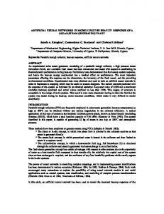
ANN techniques are conceived from our best guesses about the working of the nervous systems of animals and man. Underlying this mimicking attempt is the wish to reproduce its power and flexibility in an artificial way [after Kohonen, 1987]. However, there is (probably) little resemblance between the operation of ANNs and the operation of a nervous system like the brain. This is mainly due to our limited insights in the workings of the nervous systems and due to the fact that artificial neurons are too much of a simplification of their real-world counterparts. Biological neural networks like nervous systems can receive information from the senses at different locations in the network. This information travels from neuron to neuron through the network, after which a proper response to the information is generated. Biological neurons pass information to each other by releasing chemicals, which cause a synapse (a connection between neurons) to conduct an electric current. The receiving neuron can either pass this information to other neurons in the network or neglect its input, which causes damping of the impact of the information. This is an important characteristic of neurons, and the artificial counterparts of biological neurons replicate it to a certain degree. There are many variations on the basic type of neuron, but all biological neurons have the same four basic components as shown in Figure 2.1. The operations of biological neurons are not yet fully understood. Consequently, about a network with vast amounts of neurons (like brains) we Dendrite - Accept input signal only have primitive knowledge of its most basic Soma - Process the input signals functions. Still, there is much to learn from what Axon Turn processed inputs into outputs we do know. This knowledge can aid in the Synapse Transmit signals to other neurons development and refinement of neural computing techniques. Figure 2.1 - A biological neuron Since neuroscientists keep developing new functional concepts and models of the brain in order to increase their understanding of the brain, scientists in the field of neural computing can profit from these ideas in developing new ANN techniques. And it works the other way around, too: development of new ANN architectures, as well as concepts and theories to explain the operation of these architectures can lead to useful insights for neuroscientists. The similarity between the nervous system and ANNs becomes clearer when comparing the description of biological neurons above with the description of the ANN framework in §2.2.
§2.1.3
Evolution of ANN techniques
Many developments in computation and neuroscience in the late nineteenth and early twentieth century came together in the work of W.S. McCulloch and W.A. Pitts. Their fundamental research on the theory of neural computing in the early 1940’s led to the first neural models. Many theories about ANN techniques were further elaborated in the following decade. The advances that were made, led to the building of the first neural computers. The first successful neurocomputer was the Mark I Perceptron, which was built by Rosenblatt in 1958. Many other implementations of neurocomputers were built in the 1960’s. In 1969, a theoretical analysis by Minsky and Papert revealed significant limitations of simple models like the Perceptron and many scientists in the field of neural computing were discouraged in doing further research. Kohonen [1987] claims that the lack of computational resources and the 4
Artificial Neural Networks unsuccessful attempts to develop techniques that could solve problems on a larger scale were other reasons for the severely diminished amount of research in the field of neurocomputing. Halfway the 1980’s, interest in ANNs increased significantly, thanks to J.J. Hopfield, who became the leading force in the revitalisation of neural computing. During the following years, many of the former limitations of ANNs were overcome. The improvements on existing ANN techniques in combination with the increase in computational resources led to successful application of ANNs for many problems. One of the most groundbreaking rediscoveries was that of backpropagation techniques (which were conceived by Rosenblatt) by McClelland and Rumelhart in 1986. These developments led to an explosive growth of the field of ANNs. The number of conferences, books, journals and publications has expanded quickly since this new era. ANNs are typically used for modelling complex relations in situations where insufficient knowledge of the system under investigation is available for the use of conventional models, or if development of a conventional model is too expensive in terms of time and money. ANNs have been applied in various fields where this situation is encountered. Some examples of fields of work that show the broad possibilities of ANNs are: process control (e.g. robotics, speech recognition), economy (e.g. currency price prediction) and the military (e.g. sonar, radar and image signal processing). In spite of this broad range of applications, it is safe to say that the field is still in a relatively early stage of development.
§2.2
Framework for ANNs
In this section the theoretical building blocks for ANNs, the way they work, complement each other and how they (on a larger scale) form a functional ANN are discussed.
§2.2.1
General framework description
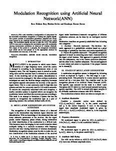
According to Rumelhart, Hinton and McClelland [1986], there are eight major components of parallel distributed processing models like ANNs: 1. A set of processing elements (neurons)2; 2. A state of activation; 3. An output function for each neuron; 4. A pattern of connectivity among neurons; 5. A propagation rule for propagating patterns of activities through the network of connectivities; 6. An activation rule for combining the inputs impinging on a neuron with the current state of that neuron to produce a new level of activation for the neuron; 7. A learning rule whereby patterns of connectivity are modified by experience; 8. An environment within which the system must operate. Some of the relations between these components are visualised in Figure 2.2. This figure depicts a schematisation of two artificial neurons and the transformations that take place between input and output. Let us assume a set of processing elements (neurons); at each point in time, each neuron ui has an activation value, denoted in the diagram as ai (t ) ; this activation value is passed trough a function
fi to produce an output value oi (t ) . This output value can be seen as passing through a set of unidirectional connections to other neurons in the system. What is associated with each connection is a real number − usually called the weight of the connection, designated wij − which determines the amount of effect that the first neuron has on the second. All of the inputs must then be combined by some operator (usually addition), after which the combined inputs to a neuron, along with its current activation value, determine its new activation value via a function Fi . Finally, the weights of these systems can undergo modification as a function of experience. This is the way the system can adapt its behaviour, aiming for a better performance.
2
The term neuron will be used from here on when referring to artificial neurons. The use of this more concise term is justified by the fact that within the context of Artificial Neural Networks a reference to neurons obviously bears reference to artificial neurons. 5
Chapter 2
Figure 2.2 - Schematic representation of two artificial neurons and their internal processes [after Rumelhart, Hinton and McClelland, 1986]
Characteristics and examples of the above mentioned components of ANNs will be presented in the following subsections in more detail. The basic structure of these sections is also based on the work of Rumelhart, Hinton and McClelland [1986].
§2.2.2
Neurons and layers
Neurons are the relatively simple computational elements that are the basic building blocks for ANNs. Neurons can also be referred to as processing elements or nodes. They are typically arranged in layers (see Figure 2.3). By convention the inputs that receive the data are called the input units3, and the layer that transmits data out of the ANN is called the output layer. Internal layers, where intermediate internal processing takes place, are traditionally called hidden layers [after Dhar and Stein, 1997]. There are as many input units and output neurons as there are input and output variables respectively. Hidden layers can contain any number of neurons. Not all networks have hidden layers. Neurons are usually indicated by circles in diagrams, and connections between neurons by lines or arrows. Input units will be depicted as squares or small circles to make a clear differentiation between these units and hidden or output neurons.
3
In some works the input units are referred to as input neurons within an input layer. Since these units serve no purpose but to pass information to the network (without the transformation of data performed by regular neurons), the author will label them input units and will disregard the whole of these units as a network layer. 6
Artificial Neural Networks
Figure 2.3 - An example of a three-layer ANN, showing neurons arranged in layers.
§2.2.3
State of activation
The state of the system at a certain point in time is represented by the state of activation of the neurons of a network. If we let N be the number of neurons, the state of a system can be represented by a vector of N real numbers, a(t ) , which specifies the state of activation of the neurons in a network. Depending on the ANN model, activation values may be of any mathematical type (integer, real number, complex number, Boolean, et cetera). Continuous activation types may be bounded within a certain interval.
§2.2.4
Output of the neurons
Neurons interact by transmitting signals to their neighbours. The strength of their signals is determined by their degree of activation. Each neuron has an output function that maps the current state of activation to an output signal: oi (t ) = f (ai (t )) (1.1) This output function is often either the identity function f ( x ) = x (so that the current activation value is passed on to other neurons), or some sort of threshold function (so that a neuron has no effect on other neurons unless its activation exceeds a certain value). The set of current output values is represented by a vector o(t ) . N.B. The output function is related to what is often called the bias of a neuron. A situation where the output function is equal to the identity function is referred to as a situation where “no bias for the neuron is used”. A bias of 0.5 basically means that a threshold function is used for the output function that the signal is only passed through the neuron if its input value exceeds 0.5.
§2.2.5
Pattern of connectivity
Neurons are connected to one another. Basically, it is this pattern of connectivity that determines how a network will respond to an arbitrary input. The connections between neurons vary in strength. In many cases we assume that the inputs from all of the incoming neurons are simply multiplied by a weight and summed to get the overall input to that neuron. In this case the total pattern of connectivity can be expressed by specifying each of the weights in the system. It is not necessary for a neuron to be connected to all neurons in the following layer. Therefore, zero values for these weights can occur. 7
Chapter 2 It is often convenient to use a matrix W for expressing all weights in the system, as the figure below shows.
⎡ ⎢w ⎢ 11 w12 ... W = ⎢ w21 w22 ... ⎢ ... ... ⎢... ⎢⎣ wN 1 wN 2 ...
⎤ w1n ⎥⎥ w2 n ⎥ ⎥ ... ⎥ wNn ⎥⎦
Weight w21 , for example, is the weight by which the output of the first node in a layer is multiplied with when it is transmitted to the second node in the successive layer.
Figure 2.4 - Illustration of network weights and the accompanying weight matrix [after HechtNielsen, 1990].
Sometimes a more complex pattern of connectivity is required. A given neuron may receive inputs of different kinds whose effects are separately summated. In such cases it is convenient to have separate connectivity matrices for each kind of connection. Connections between neurons are often classified by their direction in the network architecture: Feedforward connections are connections between neurons in consecutive layers. They are directed from input to output. Lateral connections are connections between neurons in the same layer. Recurrent connections are connections to a neuron in a previous layer. They are directed from output to input.
§2.2.6
Propagation rule
The propagation rule of a network describes the way the so-called net input of a neuron is calculated from several outputs of neighbouring neurons. Typically, this net input is the weighted sum of the inputs to the neuron, i.e. the output of the previous nodes multiplied with the weights in the weight matrix: net (t ) = W ⋅ o(t ) (1.2)
§2.2.7
Activation rule
The activation rule − often called transfer function − determines the new activation value of a neuron based on the net input (and sometimes the previous activation value, in case a memory is used). The function F , which takes a(t ) and the vectors net for each different type of connection, produces a new state of activation. F can vary from a simple identity function, so that a(t + 1) = net (t ) = W ⋅ o(t ) , to variations of linear and even non-linear functions like sigmoid functions. The most common transfer functions are listed below:
8
Artificial Neural Networks
Linear activation function:
a(t + 1) = Flin (net (t )) = α ⋅ net (t )
(1.3)
Figure 2.5 - Linear activation function.
Hard limiter activation function:
⎧α a(t + 1) = Fhl (net (t )) = ⎨ ⎩β
if
net (t ) < z net (t ) ≥ z
(1.4)
Figure 2.6 - Hard limiter activation function.
Saturating linear activation function:
α ⎧ ⎪ a(t + 1) = Fsl (net (t )) = ⎨net (t ) + γ ⎪ β ⎩
if
net(t) < z z ≤ net(t) ≤ y net(t) > y
(1.5)
Figure 2.7 - Saturating linear activation function.
9
Chapter 2
Gaussian activation function:
a(t + 1) = Fbs (net (t )) = e
−
( net ( t ) )2 α
(1.6)
where α is a parameter that defines the wideness of the Gauss curve, as illustrated below.
Figure 2.8 - Gaussian activation function for three different values of the wideness parameter.
Binary sigmoid activation function:
a(t + 1) = Fbs (net (t )) =
1 1+ e
−α ⋅net ( t )
(1.7)
where α is the slope parameter of the function. By varying this parameter, different shapes of the function can be obtained, as illustrated below.
Figure 2.9 - Binary sigmoid activation function for three different values of the slope parameter.
10
Artificial Neural Networks
Hyperbolic tangent sigmoid activation function:
a(t + 1) = Fbs (net (t )) = tanh(net (t ))
(1.8)
Figure 2.10 - Hyperbolic tangent sigmoid activation function.
§2.2.8
Learning
Based on sample data that is presented to it during a training stage, an ANN will attempt to learn the relations that are contained within the sample data by adjusting its internal parameters (i.e. the weights of the connections in the network and the neuron biases). This means that the relations that need to be approximated are parameterised in the ANN structure. The way a network is trained is a basic property of an ANN; the values of several neuron properties and the manner in which the neurons of an ANN are structured are closely related to the chosen algorithm. The algorithm that is used to optimise these weights and biases is called training algorithm or learning algorithm. Training algorithms can be classified broadly into those comprising supervised learning and unsupervised learning. Supervised learning works by presenting the ANN with input data and the desired correct -
output results. This is done by an external ‘teacher’, hence the name of this method. The network generates an estimate, based on the given input, and then compares its output with the desired results. This information is used to help guide the ANN to a good solution. Some learning methods do not present the actual desired value of the output to the network, but rather give an indication of the correctness of the estimate. [after Dhar and Stein, 1997]
N.B. These learning methods have a clear relation with the process of calibration, which is used in many conventional modelling techniques. This becomes clear when comparing the above with what Rientjes and Boekelman [2001], for example, state: “a procedure of adjusting model parameter values is necessary to match model output with measured data for the selected period and situation entered to the model. This process of (re)adjustment and (re)calculating is termed calibration and deals about finding the most optimal set of model parameters.” -
ANNs being trained using an unsupervised learning paradigm are only presented with the input data but not the desired results. The network clusters the training records based on similarities that it abstracts from the input data. The network is not being supervised with respect to what it is ‘supposed’ to find and it is up to the network to discover possible relationships from the input data and based on this make certain predictions of an output. [after Dhar and Stein, 1997]
11
Chapter 2 Supervised and unsupervised learning can be further divided into different classes, as shown in Table 2.1 and Table 2.2. Performance learning techniques is the best known category of supervised learning, as competitive learning is of unsupervised learning. Table 2.1 - Overview of supervised learning techniques
Supervised learning Performance learning Backpropagation Methods based on statistical optimisation algorithms: o Conjugate gradient algorithms o (Quasi-) Newton’s algorithm o (Reduced) Levenberg-Marquardt algorithm Cascade-Correlation algorithm
Coincidence learning Hebbian learning
Table 2.2 - Overview of unsupervised learning techniques
Unsupervised learning Competitive learning Kohonen learning Adaptive Resonance Theory (ART)
Filter learning Grossberg learning
Only performance learning algorithms will be discussed in the following section since these are the only algorithms used throughout this investigation. Performance learning algorithms An ANN that is trained using a supervised learning method attempts to find optimal internal parameters (weights and biases) by comparing its own approximations of a process with the real values of that process and subsequently adjusting its weights (and biases4) to make its approximation closer to the real value. The aforementioned comparison is based upon an evaluation using a performance function (hence the name performance learning). The author will refer to this function as error function5. Suppose a network is trying to approximate a certain process, which can be characterised by a number of n variables (see Figure 2.11). The network input is a vector x and the weights of the network form a matrix W ). The approximation of the network is a vector of n variables called y = ( y1 , y2 ,..., yn ) (which is a function of x and W ) and the real values of the variables are included in a vector called t = (t1 , t2 ,..., tn ) . The difference between the two is used to calculate an approximation error E . In order for an ANN to generate an output vector y that is as close as possible to the target vector t , an algorithm is employed to find optimal internal parameters that minimize an error function. This function usually has the form: n
E = ∑ ( t h − yh )
2
(1.9)
h =1
where n is the number of output neurons. [after Govindaraju, 2000]
4
The use of biases is not very common. Training of an ANN often only comes down to updating the network weights. From this point on, the author will ignore biases in the discussion about the training process. 5 The name performance function is somewhat deceptive since it basically is a function that expresses the value of the residual errors of the ANN. Since the function is minimized during ANN training the term error function is preferable. 12
Artificial Neural Networks
Figure 2.11 - Example of a two-layer feedforward network.
Equation (1.9) is based on the error expression called Mean Square Error (MSE). The MSE error measurement scheme is often used, because it has certain advantages. Firstly, it ensures that large errors receive much greater attention than small errors, which is usually what is desired. Secondly, the MSE takes into account the frequency of occurrence of particular inputs. The MSE is best used if errors are near normally distributed. Other residual error measures can be more appropriate if, for instance, evaluating errors that are not normally distributed or when examining specific aspects of a process that require a different error measure. Examples of alternative error measures are the mean absolute error (e.g. used if approximating the mean of a certain process is somewhat more important than approximating the process in its complete range, i.e. including minima and maxima) and variants of the MSE, such as the Rooted Mean Squared Error (RMSE). Consult §3.8.1 for the equations of these errors. Because y is a function of the weights in W the error function ( E ) also becomes a function of W of the network being evaluated. For each combination of weights a different residual error arises. These errors can be visualized by plotting them in an extra dimension in addition to the dimensions of the weight space of the network. For example: assume a network with two weights, w1 and w2 . The two-dimensional weight space can be expanded with a third dimension in which the residual error E for each combination of the weights w1 and w2 is expressed. The result can be plotted as a threedimensional surface (as is done in Figure 2.12). The points on this error surface are specified by three coordinates: the value of w1 , the value of w2 and the value of the error E for this combination of w1 and w2 . The goal for learning algorithms is to find the lowest point on this surface, meaning the weight vector where the residual error is minimal. We can visualize the effect of a good algorithm as a ball rolling towards a minimum on the surface (see Figure 2.12). Note that the shape of the error surface depends on the error function used.
13
Chapter 2
Figure 2.12 - Example of an error surface above a two-dimensional weight space. A good training algorithm can be thought of as a ball ‘rolling’ towards a minimum. [after Dhar and Stein, 1997]
The starting point, from which a training algorithm tries to find a minimum, is determined by the initial values of the weights in the network at the start of the training. These weights are often set at small random values (see §3.7.1). Performance learning algorithms can update the ANN weights right after processing each training sample. Another possibility is updating the network weights only after processing the entire training data set and making the accompanying calculations. This update is commonly formed as an average of the corrections for each individual training sample. This method is called batch training or batch updating. Past applications have proven this method to be more suitable if a more sophisticated algorithm is used. If batch learning is used, the error function that has to be minimized has the form p
n
E = ∑∑ ( tqh − yqh )
2
(1.10)
q =1 h =1
where n is the number of output neurons and p the number of training patterns. Batch updating introduces a filtering effect to the training of an ANN, which in some cases can be beneficial. This approach, however, requires more memory and adds extra computational complexity. In general, the performance of a batch-updating algorithm is very case-dependant. A good compromise between step-by-step updating and batch updating is to accumulate the changes over several, but not all, training pairs before the weights are updated. N.B. All learning algorithms attempt to find the optimal set of internal network parameters, i.e. the global minimum of the error function. However, there may be more than one global minima of this function, so that more than one parameter set exist that approximate the training data optimally. Besides global minima, error functions often feature multiple local minima. It is important for an ANN researcher to
14
Artificial Neural Networks realize that it is very difficult to tell with certainty whether a trained network has reached a local minimum or a global minimum. The following sections provide more details about various performance learning algorithms. The stepby-step descriptions of these algorithms can be found in Appendix B. Standard backpropagation The best-known algorithm for training ANNs is the backpropagation algorithm. It essentially searches for minima on the error surface by applying a steepest-descent gradient technique. The algorithm is linearly convergent. The backpropagation architecture described here and in the accompanying appendices is the basic, classical version, but many variants of this basic form exist. Basically, each input pattern of the training data set is passed through a feedforward network from the input units to the output layer. The network output is compared with the desired target output, and an error is computed based on an error function. This error is propagated backward through the network to each neuron, and correspondingly the connection weights are adjusted. Backpropagation is a first-order method based on the steepest gradient descent, with the direction vector being set equal to the negative of the gradient vector. Consequently, the solution often follows a zigzag path while trying to reach a minimum error position, which may slow down the training process. It is also possible for the training process to be trapped in a local minimum. [after Govindaraju, 2000] See Appendix A for the derivation of the backpropagation algorithm and Appendix B for a step-by-step description of the backpropagation algorithm. N.B. One parameter used with (backpropagation) learning deserves special attention: the so-called learning rate. The learning rate can be altered to increase the chance of avoiding the training process being trapped in local minima instead of global minima. Many learning paradigms make use of a learning rate factor. If a learning rate is set too high, the learning rule can ‘jump over’ an optimal solution, but too small a learning factor can result in a learning procedure that evolves too gradual. The learning rate is an interesting parameter for ANN training. Some learning methods use a variable learning rate in order to improve their performance. Appendix B provides more mathematical detail about the learning rate. The parameter can be found in several other weight updating formulas besides the backpropagation algorithm. Conjugate gradient algorithms The conjugate gradient method is a well-known numerical technique used for solving various optimisation problems. It is widely used since it represents a good compromise between simplicity of the steepest descent algorithm and the fast quadratic convergence of Newton’s method (see following sections on (quasi-)Newton and Levenberg-Marquardt algorithms). Many variations of the conjugate gradient algorithm have been developed, but its classical form is discussed below and in Appendix B. The conjugate gradient method, unlike standard backpropagation, does not proceed along the direction of the error gradient, but in a direction orthogonal to the one in the previous step. This prevents future steps from influencing the minimization achieved during the current step. It is proven that any minimization method developed by the conjugate gradient algorithm is quadratically convergent. Appendix B provides a step-by-step description of the conjugate gradient algorithm. (Quasi-)Newton algorithms According to Newton’s method, the set of optimal weights that minimizes the error function can be found by applying: w ( k + 1) = w (k ) − H −k 1 ⋅ g k (1.11)
15
Chapter 2 where H k is the Hessian matrix (second derivatives) of the performance index at the current values of the weights and biases:
H k = ∇ 2 E (w )
w =w (k )
⎡ δ 2 E (w ) ⎢ 2 ⎢ δ w1 ⎢ δ 2 E (w ) ⎢ = ⎢ δ w2 ⋅ δ w1 ⎢ ... ⎢ 2 ⎢ δ E (w ) ⎢ ⎣ δ wN ⋅ δ w1
δ 2 E (w ) δ w1 ⋅ δ w2
...
δ 2 E (w ) δ w2 2
...
...
...
δ E (w ) δ wN ⋅ δ w2
...
δ 2 E (w ) ⎤ δ w1 ⋅ δ wN ⎥⎥
δ 2 E (w ) ⎥ ⎥ δ w2 ⋅ δ wN ⎥
2
(1.12)
⎥ ... ⎥ δ 2 E (w ) ⎥ ⎥ δ wN 2 ⎦ w = w ( k )
and g k represents the gradient of the error function:
g k = ∇E ( w ) w = w ( k )
⎡ δ E (w) ⎤ ⎢ δw ⎥ 1 ⎢ ⎥ ⎢ δ E (w) ⎥ ⎢ ⎥ = ⎢ δ w2 ⎥ ⎢ ... ⎥ ⎢ ⎥ ⎢ δ E (w) ⎥ ⎢⎣ δ wN ⎥⎦ w =w (k )
(1.13)
Newton’s method can (theoretically) converge faster than conjugate gradient methods. Unfortunately, the complex nature of the Hessian matrix can make it resource-intensive to compute. Quasi-Newton methods offer a solution to this problem with less computational requirements: they update an approximate Hessian matrix at each iteration of the algorithm, thereby speeding up computations during the learning process. [after Govindaraju, 2000] Appendix B contains a step-by-step algorithm of a typical quasi-Newton algorithm, namely the Broyden-Fletcher-Goldfarb-Shanno (BFGS) algorithm. Levenberg-Marquardt algorithm Like other quasi-Newton methods, the Levenberg-Marquardt algorithm was designed to approach second-order training speed without having to compute the Hessian matrix. If the performance function has the form of a sum of squares, then the Hessian matrix can be approximated as H = JT J (1.14) and the gradient can be computed as
g = JT e
(1.15)
where J is the Jacobian matrix and e is a vector of network errors.
⎡ δ e1 ⎢δ w ⎢ 1 ⎢ δ e2 ⎢ J = ⎢ δ w1 ⎢ ... ⎢ ⎢ δ eP ⎢⎣ δ w1
δ e1 δ w2 δ e2 δ w2 ... δ eP δ w2
δ e1 ⎤ δ wN ⎥ ⎥ δ e2 ⎥ ... δ wN ⎥⎥ ...
...
... δ eP ... δ wN
(1.16)
⎥ ⎥ ⎥ ⎥⎦
The Jacobian matrix contains first derivatives of the network errors with respect to the weights and biases. The Jacobian matrix is less complex to solve than the Hessian matrix.
16
Artificial Neural Networks One problem with this method is that it requires the inversion of matrix H = J T J , which may be illconditioned or even singular. This problem can be easily resolved by the following modification: H = JT J + µ ⋅ I (1.17) where µ is a small number and I is the identity matrix. This method represents a transition between the steepest descent method and Newton’s method. It makes an attempt at combining the strong points of both methods (fast initial convergence and fast/accurate convergence near an error minimum, respectively) into one algorithm. A step-by-step description of the Levenberg-Marquardt algorithm can be found in Appendix B. Quickprop algorithm The Quickprop algorithm, developed by Fahlman [1988], is a well-known modification of backpropagation. It is a second-order method based on Newton’s method. The weight update procedure depends on two approximations: first, that small changes in one weight have relatively little effect on the error gradient observed at other weights; second, that the error function with respect to each weight is locally quadratic. Quickprop tries to jump to the minimum point of the quadratic function (parabola). This new point will probably not be the precise minimum, but as a single step in an iterative process the algorithm seems to work very well, according to Fahlman and Lebiere [1991]. A step-by-step description of the Quickprop algorithm can be found in Appendix B. Cascade-Correlation algorithm Fahlman and Lebiere developed the Cascade-Correlation algorithm in 1990. The Cascade-Correlation algorithm is a so-called meta-algorithm or constructive algorithm. The algorithm not only trains the network by minimizing the network error by adjusting internal parameters (much like any other training algorithm) but it also attempts to find an optimal network architecture by adding neurons to the network. A training cycle is divided into two phases. First, the output neurons are trained to minimize the total output error. Then a new neuron (a so-called candidate neuron) is inserted and connected to every output neuron and all neurons in the preceding layer (in effect, adding a new layer to the network). The candidate neuron is trained to correlate with the output error. The addition of new candidate neurons is continued until maximum correlation between the hidden neurons and error is attained. Instead of training the network to maximize the correlation between the output of the neurons and the output error, one can also choose to train to minimize the output error of the ANN. This variant of Cascade Correlation is mostly used in function approximation applications. A step-by-step description of the Cascade-Correlation algorithm and a discussion of several variants of it can be found in Appendix B.
§2.2.9
Representation of the environment
The model of the environment, in which an ANN is to exist, is a time-varying stochastic function over the space of input patterns. That is, we imagine that at any point in time, there is some probability that any of the possible set of input patterns is impinging on the input units. This probability function may in general depend on the history of inputs to the system as well as output of the system.
§2.3
Function mapping capabilities of ANNs
The approximation of mathematical functions is often referred to as (function) mapping. The majority of ANN applications make use of the mapping capabilities of ANNs. This survey will provides more detail on function mapping since this is also the main focus of this investigation. After an introduction in function mapping, two types of mapping networks will be discussed: standard feedforward networks (§2.3.2) and radial basis function networks (§2.3.3). The implementation of the dimension of time in ANNs is discussed in §2.3.4.
17
Chapter 2
§2.3.1
About function mapping
Mapping ANN
x
f
x ∈ℜn×1
y
y ∈ℜm×1
Figure 2.13 - General structure for function mapping ANNs [after Ham and Kostanic, 2001].
The problem addressed by ANNs with mapping capabilities is the approximate implementation of a bounded mapping or function f : A ⊂ R n → R m , from a bounded subset A of n -dimensional Euclidean space to a bounded subset f [ A] of m -dimensional Euclidean space, by means of training on examples ( x1 , t1 ) , ( x 2 , t 2 ) , ...
( xk , t k )
of the mapping’s action, where t k = f ( x k ) [after Hecht-
Nielsen, 1990]. Mapping networks can also handle the case where noise is added to the examples of the function being approximated. The approximation accuracy of a mapping ANN is measured by comparing its output ( y ) for a certain input signal ( x ) with the target values ( t ) from the data set. Hecht-Nielsen [1990] states that the manner in which mapping networks approximate functions can be thought of as a generalization of statistical regression analysis. A simple linear regression model, for example, is based on an estimated linear functional form, from which variations occur by different slope and intercept parameters, which are determined using the construction data set. The biased function form and variations thereof in an ANN model are less well defined: Regression analysis techniques require the researcher to choose the form of a function to be fitted to data, while ANN techniques do not. ANNs have many more free internal parameters (each trainable weight) than corresponding statistical models (as a result, they are tolerant of redundancy). What is important to realize is that in both cases the form of the function f will not be revealed explicitly. The function form is implicitly represented in the slope and intercept parameters in the case of linear regression analysis and in the network’s internal parameters in the case of ANNs. There are several types of ANNs that can be designated as mapping networks. The author, however, will follow the strict definition of mapping networks presented above. This results in an exclusion, for example, of the so-called linear associator networks (which can be seen as simplified mapping networks) and the so-called self-organizing maps (which can be seen as unsupervised learning variants of standard mapping networks). The following two subsections will focus only on the most commonly used function mapping ANNs: standard feedforward networks, radial basis function networks and temporal networks6.
§2.3.2
Standard feedforward networks
Most mapping networks can be designated standard feedforward networks. The number of variations of these ANNs is vast. The most important characteristic of standard feedforward networks is that (as the name suggests) the only types of connections during the operational phase are feedforward connections (explained in §2.2.5). Note that during the learning phase feedback connections do exist to propagate output errors back into the ANN (as discussed in §2.2.8). A standard feedforward network may be built up from any number of hidden layers, or there may only be input units and an output layer. The training algorithm used can be any kind of supervised 6
Other ANNs that exhibit mapping capabilities exist (e.g. the counterpropagation network [Hecht-Nielsen, 1990]), but have been disregarded here because they are seldom used. 18
Artificial Neural Networks learning algorithm. All other ANN architecture parameters (number of neurons in each layer, activation function, use of a neuron bias, et cetera) may vary. Multilayer perceptrons Feedforward networks with one or more hidden layers are often addressed in literature as multilayer perceptrons (MLPs). This name suggests that these networks consist of perceptrons (named after the Perceptron neurocomputer developed in the 1950’s, discussed in §2.1.3). The classic perceptron is a neuron that is able to separate two classes based on certain attributes of the neuron input. Combining more than one perceptron results in a network that is able to make more complex classifications. This ability to classify is partially based on the use of a hard limiter activation function (see §2.2.7). The activation function of neurons in feedforward networks, however, is not limited to just hard limiter functions; sigmoid or linear functions (see §2.2.7) are often used too. And there are often other differences between perceptrons and other types of neurons. From this we can conclude that the name MLP for multilayer feedforward networks consisting of regular neurons (not perceptrons, which are neurons with specific properties) is therefore basically incorrect. To avoid misunderstandings, the author will not use the term MLP for a standard feedforward networks with one or more hidden layers (unless of course their neurons do function like the classic form of the perceptron). Backpropagation networks Feedforward networks are sometimes referred to with a name that is derived from the employed training algorithm. The most common learning rule is the backpropagation algorithm. An ANN that uses this learning algorithm is consequently referred to as a backpropagation network (BPN). One must bear in mind, however, that different types of ANNs (other than feedforward networks) can also be trained using the backpropagation algorithm. These networks should never be referred to as backpropagation networks, for the sake of clarity. It is for the same reason, that the author will not use a term such as ‘backpropagation network’ in this report, but will refer to such an ANN by its proper name: backpropagation-trained feedforward network.
§2.3.3
Radial basis function networks
The Radial Basis Function (RBF) network is a variant of the standard feedforward network. It can be considered as a two-layer feedforward network in which the hidden layer performs a fixed non-linear transformation with no adjustable internal parameters. The output layer, which contains the only adjustable weights in the network, then linearly combines the outputs of the hidden neurons [after Chen et al., 1991]. The RBF network is trained by determining the connection weights between the hidden and output layer through a performance training algorithm. The hidden layer consists of a number of neurons and internal parameter vectors called ‘centres’, which can be considered the weight vectors of the hidden neurons. A neuron (and thus a centre) is added to the network for each training sample presented to the network. The input for each neuron in this layer is equal to the Euclidean distance between an input vector and its weight vector (centre), multiplied by the neuron bias. The transfer function of the radial basis neurons typically has a Gaussian shape (see §2.2.7). This means that if the vector distance between input and centre decreases, the neuron’s output increases (with a maximum of 1). In contrast, radial basis neurons with weight vectors that are quite different from the input vector have outputs near zero. These small outputs only have a negligible effect on the linear output neurons. If a neuron has an output of 1 the weight values between the hidden and output layer are passed to the linear output neurons. In fact, if only one radial basis neuron had an output of 1, and all others had outputs of 0's (or very close to 0), the output of the linear output layer would be the weights between the active neuron and the output layer. This would, however, be an extreme case. Typically several neurons are always firing, to varying degrees. Summarising, a RBF network determines the likeness between an input vector and the network’s centres. It consequently produces an output based on a combination of activated neurons (i.e. centres that show a likeness) and the weights between these hidden neurons and the output layer. The primary difference between the RBF network and backpropagation lies in the nature of the nonlinearities associated with hidden neurons. The nonlinearity in backpropagation is implemented by a fixed function such as a sigmoid. The RBF method, on the other hand, bases its nonlinearities on the 19
Chapter 2 data in the training set [after Govindaraju, 2000]. The original RBF method requires that there be as many RBF centres (neurons) as training data points, which is rarely practical, since the number of data points is usually very large [after Chen et al., 1991]. A solution to this problem is to monitor the total network error while presenting training data (adding neurons), and to stop this procedure when the error does no longer significantly decrease. RBF networks are generally capable of reaching the same performance as feedforward networks while learning faster. On the downside, more data is required to reach the same accuracy as feedforward networks. According to Chen, Cowan and Grant [1991], RBF network performance critically depends on the centres that result from the inputted training data. In practice, these training data are often chosen to be a subset of the total data, which suitably samples the input domain.
§2.3.4
Temporal ANNs
When a function mapping ANN tries to approximate a time-dependant function (e.g. in a ANN speech system), the dimension of time needs to be incorporated into the network for optimal performance. ANN models in which the time dimension is implemented one way or another are called temporal ANNs.
Temporal ANNs Time externally processed = Static ANNs (TDNNs, pp. 20)
Time as internal mechanism = Dynamic ANNs
Implicit time = Partially recurrent ANNs (SRNs, pp. 22)
Time at the network level (DTLFNNs, pp. 21)
Time explicitly represented in the architecture = Fully recurrent ANNs
Time at the neuron level (continuous-time ANNs)
Figure 2.14 - A classification of ANN models with respect to time integration [modified after Chappelier and Grumbach, 1994]. The pages that are referred to are the pages on which these temporal ANN examples are discussed.
With respect to the integration of the time dimension into ANN models, the first option is not to introduce it at all but to leave time outside the ANN model (which is consequently named a static network). Models that incorporate this method are called tapped delay line models. This method comes down to inputting a window of input series to a network, i.e. P ( t ) , P ( t − 1) , ... , P ( t − m ) .
P ( t ) represents one of the inputs at time t and m the memory length. The total of input neurons increases with the length of the memory used. Presenting an ANN with a tapped delay line basically means that the temporal pattern is converted to a spatial pattern, which can then be learned by a static network. This method can also be combined with one of the dynamic network types that are discussed below. This is typically the case if predicting multiple time steps ahead, which is discussed from page 23 on. The introduction of the time dimension in a neural model by incorporating it in the ANN architecture (which means the ANN becomes a dynamic network) can be made at several levels. First of all, time can be used as an index of network states. The preceding state of neurons is preserved and
20
Artificial Neural Networks reintroduced at the following step at any point in the network. Order is the only property of time used when working with these sequences. Chappelier and Grumbach [1994] call this an implicit presentation of time into the models. This method basically means that the neurons of a layer within an ANN can be connected to neurons of the preceding layer, the succeeding layer and the layer itself. These types of models are referred to as context models or partially recurrent models. Note that the weight updating for a context model is not local, in the sense that updating of a single weight requires the manipulation of the entire weight matrix, which in turn increases the computational effort and time. A step further in the introduction of the time dimension in an ANN is to represent it explicitly at the level of the network, i.e. by introducing some delays of propagation (time weights) on the connections and/or by introducing memories at the level of the neuron itself. These models are referred to as fully recurrent models. Algorithms to train these dynamic models are significantly more complex in terms of time and storage requirements. In the case of time implementation at the network level, ANNs use the combination of an array to represent the connection strength between two neurons of consecutive layers (instead of a single weight value), and internal delays. Elements of the array are the weights for present and previous inputs to the neuron. Such an array is called a Finite Impulse Response (FIR). What is finally mentioned in the classification diagram above, is time at the neuron level. This method requires a continuous approach, which will not be discussed here. Because of the recurrent connections in dynamic networks, variations of the regular training algorithms must be used when training a dynamic network. Two well-known examples of dynamic learning algorithms are the Backpropagation Through Time (BPTT) algorithm [Rumelhart et al., 1986] and the Real-Time Recurrent Learning (RTRL) algorithm [Williams and Zipser, 1989]. Temporal network examples The following review shows the most common types of temporal networks as described by Ham and Kostanic [2001]. The classification of these networks is shown in Figure 2.14.
Time-delay neural network (TDNN) The TDNN is actually a feedforward multilayer network with the inputs to the network successively delayed in time using tapped delay lines. Figure 2.15 shows a single neuron with multiple delays for each element of the input vector. This is a neuron ‘building block’ for feedforward TDNNs. As the input vector x ( k ) evolves in time, the past p values are accounted for in the neuron. A temporal sequence, or time window, for the input is established and can be expressed as
X = {x ( 0 ) , x (1) ,..., x ( m )}
(1.18)
Within the structure of the neuron the past values of the input are established by the way of the time delays shown in Figure 2.15 (for p < m ). The total number of weights required for the single neuron is
( p + 1) n .
21
Chapter 2
Figure 2.15 - Basic TDNN neuron with n connections from input units and p delays on each input signal (k is the discrete-time index) [after Ham and Kostanic, 2001].
The single-neuron model can be extended to a multilayer structure. The typical structure of the TDNN is a layered architecture with only delays at the input of the network, but it is possible to incorporate delays between the layers.
Distributed time-lagged feedforward neural network (DTLFNN)
A DTLFNN is distributed in the sense that the element of time is distributed throughout the ANN architecture by time weights on the internal network connections. Opposed to the implicit method used by partially recurrent networks, DTLFNNs have time explicitly represented in the network architecture by Finite Impulse Responses (FIRs), depicted in Figure 2.16. The arrays of time weights represented by the FIRs can accomplish time dependant effects by means of internal delays at every neuron.
Figure 2.16 - Non-linear neuron filter [after Ham and Kostanic, 2001]
ANNs using FIRs can be seen as closely related to static ANNs using a time window (TDNNs), since a FIR is basically a window-of-time input to a neuron. The difference is that DTLFNNs provide a more general model for time representation because FIRs are distributed through the entire network.
22
Artificial Neural Networks
Simple recurrent network (SRN)
The SRN is often referred to as the Elman network. It is a single hidden-layer feedforward network, except for the feedback connections from the output of the hidden-layer neurons to the input of the network.
Figure 2.17 - The SRN neural architecture (where z-1 is a unit time delay) [after Ham and Kostanic, 2001]
The context units in Figure 2.17 replicate the hidden-layer output signals at the previous time step, that is x ' ( k ) . The purpose of these context units is to deal with input pattern dissonance. The feedback provided by these units basically establishes a context for the current input x ( k ) . This can provide a mechanism within the network to discriminate between patterns occurring at different times that are essentially identical. The weights of the context units remain fixed. The other network weights, however, can be adjusted using the backpropagation algorithm with momentum (see Appendix B for details). Multi-step ahead predictions A subject that is closely related to the implementation of time in ANNs is that of making predictions for more than one time steps ahead. When predicting p time steps ahead, for example, the same principle can be used as when predicting a single time step ahead. Instead of training an ANN with variable values on t+1 as targets, t+p values can be used. The result is a one-stage p-step ahead predictor. However, as Duhoux [2002] mentions, this introduces an information gap, since all (estimated) information for time steps t+1…t+p-1 is not used. In this case, it is better to rely on multi-step ahead prediction methods, several of which will be discussed below. 1. Recursive multi-step method (also referred to as: iterated prediction); The network only has one output neuron, forecasting a single time step ahead, and the network is applied recursively, using the previous predictions as inputs for the subsequent 23
Chapter 2 forecasts (Figure 2.18). This method has proven useful for local modelling approaches, discussed in §3.2.3, but if a global modelling approach is taken this method can be plagued by the accumulation of errors [after Boné and Crucianu, 2002].
Figure 2.18 - The recursive multi-step method. New estimated outputs are shifted through the input vector and old inputs are discarded. All neural networks are identical. [after Duhoux et al., 2002]
2. Chaining ANNs; One can also chain several ANNs to make a multi-step ahead prediction (Figure 2.19). For a time horizon of p, a first network learns to predict at t+1, then a second network is trained to predict at t+2 by using the prediction provided by the first network as a supplementary input. This procedure is repeated until the desired time horizon p is reached. [after Boné and Crucianu, 2002]
Figure 2.19 - Chains of ANNs: beginning with a classical one-step ahead predictor, the outputs are inserted in a next one-step ahead predictor, by adding the one-step ahead prediction to the input vector of the subsequent predictor. [after Duhoux et al., 2002]
3. Direct multi-step method. The ANN model can also be trained simultaneously on both the single step and the associated multi-step ahead prediction problem. The network has several neurons in the
24
Artificial Neural Networks output layer, each of which represents one time step to be forecasted (Figure 2.20). There can be as many as p output neurons. Training is done by using an algorithm that punishes the predictor for accumulating errors in multi-step ahead prediction (e.g. the Backpropagation Through Time algorithm). This method can provide good results, especially if it is assisted by some form of implementation of time into the network architecture (e.g. recurrent connections or FIRs).
Figure 2.20 - Direct multi-step method. The ANN that is used is often a temporal network of some sort.
§2.4
Performance aspects of ANNs
This section will firstly provide an overview of the positive and negative aspects of ANN techniques, which have been encountered by historical applications of ANNs. Secondly, one of the most often encountered problems concerning ANN techniques is discussed: overtraining. The section on overtraining (§2.4.2) not only aids in a further understanding of the overtraining problem and thereby prevention of this problem, but it also provides insights that lead to a deeper understanding of ANN training techniques in general. A phenomenon that is closely related to overtraining is underfitting and is discussed in §2.4.3.
§2.4.1
Merits and drawbacks of ANNs
Previous applications of ANNs in various fields of work have given insight in the merits and drawbacks of ANN techniques as opposed to other modelling techniques. This section presents a brief overview of the strengths and limitations that have proven to be universal for ANNs. Zealand, Burn and Simonovic [1999] claim that ANNs have the following beneficial model characteristics: +
They infer solutions from data without prior knowledge of the regularities in the data; they extract the regularities empirically. This means that when ANN techniques are used in a certain field of work, relatively little specific knowledge of that field is demanded for the development of that model because of the empirical nature of ANNs. This demand is certainly higher when developing models using conventional modelling techniques.
+
These networks learn the similarities among patterns directly from examples of them. ANNs can modify their behaviour in response to the environment (i.e. shown a set of inputs with corresponding desired outputs, they self-adjust to produce consistent responses).
+ ANNs can generalize from previous examples to new ones. Generalization is useful because real-world data are noisy, distorted, and often incomplete. +
ANNs are also very good at the abstraction of essential characteristics from inputs containing irrelevant data.
+
They are non-linear, that is, they can solve some complex problems more accurately than linear techniques do.
25
Chapter 2 + Because ANNs contain many identical, independent operations that can be executed simultaneously, they are often quite fast. As mentioned earlier, ANNs belong to the family of parallel distributed processing systems, which are known to be faster than conventional models. This is of course dependant on the efficiency of the ANN. ANNs have several drawbacks for some applications too [modified after Zealand, Burn and Simonovic, 1999]: -
ANNs may fail to produce a satisfactory solution, perhaps because there is no learnable function or because the data set is insufficient in size or quality.
-
The optimal training data set, the optimum network architecture, and other ANN design parameters cannot be known beforehand. A good ANN model generally has to be found using a trial-and-error process.
-
ANNs are not very good extrapolators. Deterioration of network performance when predicting values that are outside the range of the training data is generally inevitable. Pre-processing data (discussed in §3.5.2) can help reducing this performance drop.
-
ANNs cannot cope with major changes in the system because they are trained (calibrated) on a historical data set and it is assumed that the relationship learned will be applicable in the future. If there were major changes in the system, the neural network would have to be adjusted to the new process.
-
It is impossible to tell beforehand which internal network parameter set (i.e. collection of network weights) is the optimal set for a problem. Training algorithms often do a good job of finding a parameter set that performs well, but this is not always the case, e.g. when coping with a very complex error surface for a problem. In addition to this problem, it is also very difficult to tell whether a training algorithm has found a local or a global minimum. Another problem is that for different periods in time or for different dominating processes described in the training set, there will likely be sets of parameters that give a good fit to the test data for each one of these situations and other sets giving good fits by a mixture of all the periods or processes [Beven, 2001]. The different optima may then be in very different parts of the parameter space, making matters complicated for choosing the ‘optimal’ ANN.
The lack of ‘explainablility’ of ANN model results is one of the primary reasons for the sceptical attitude towards application of ANN techniques in certain fields. The lack of physical concepts and relations is a reason for many scientists to look at ANNs with Argus’ eyes. For ANNs to gain wider acceptability, it is increasingly important that they have some explanation capability after training has been completed. Most ANN applications have been unable to explain in a comprehensive meaningful way the basic process by which ANNs arrive at a decision. [Govindaraju, 2000] A superficial review of ANN characteristics is presented in Table 2.3. What is meant with the high embeddability of ANNs in this table is the fact that it is often not too difficult to combine an ANN with another model technique. These combined models are referred to as hybrid systems. Such systems can superficially be divided into two groups: A hybrid system containing separate models that are linked in a serial or a parallel way, for instance by exchange of data files; A hybrid system that features a full integration of different techniques. Examples of other techniques with which ANNs can form a hybrid system are: numerical models, statistical models, expert systems and genetic algorithms.
26
Artificial Neural Networks
Table 2.3 - Review of ANN performance on various aspects [modified after Dhar & Stein, 1997].
Aspect Accuracy
ANN performance High
Explainability/transparency
Low
Response speed
High
Scalability
Moderate
Compactness Flexibility Embeddability Ease of use Tolerance for complexity
High High High Moderate High
Tolerance for noise in data
Moderate - high
Tolerance for sparse data Independence from experts
Low High
Development speed
Moderate
Computing resources
Low - moderate
§2.4.2
However… Needs comprehensive training data Some mathematical analytic methods exist for doing sensitivity analysis Depends on complexity of problem and availability of data Needs representative training data Pre-processing can be very useful in dealing with noise Depends on understanding of process, on computer speed, and learning method Scale with respect to amount of data and size of network. A trained ANN needs little computing resources to execute.
Overtraining
An often encountered problem when applying ANN techniques is called overtraining. Overtraining effects typically result from a combination of three (often complementary) causes: 1. Using an ANN architecture, which is too complex for the relations that are to be modelled; 2. Overly repetitive training of an ANN; 3. Training an ANN using an inappropriate training data set. Point 1 is basically an ‘overparameterisation’ problem, which is also encountered in other modelling fields. The best approximation by a model can be realised by a number of different sets of model parameter values. The uniqueness of the relations between model outputs and parameters determines a model’s degree of parameterisation. Overparameterisation means ‘losing control’ of the meaning of model parameters because the model has too many degrees of freedom (i.e. the number of possible sets of parameter values is too large). As a result, model output uncertainty is increased. Possible causes of overparameterisation are: An unbalanced rate of parameters and information (e.g. many parameters for little information); Occurrence of correlations between model parameter values; An unbalanced rate of sensitive and insensitive model parameters (e.g. too many sensitive parameters). A large (and therefore complex) ANN architecture opposed to relatively simple information, to which the ANN model adapts, is an example of a poor ratio between the number of model parameters and the complexity of data information content. As a result, the chance of overparameterisation occurring will increase. Points 2 and 3 are reasons for overtraining, because too much similar information is presented to an ANN. The ANN model adapts its internal parameters to this information, resulting in a rigid model that succeeds in approximating the relations presented in the training data, but fails to approximate the relations in other data sets with slightly different data values. Basically, the network adjusts its internal parameters based on not only the essential relations associated with the empirical data, but also unwanted effects in the data. This can result in a model 27
Chapter 2 with poor predictive capability. These unwanted effects could be associated with either measurement noise or any other features of the data associated with additional relations or phenomena that are not of any interest when designing a model. [Ham and Kostanic, 2001] Because the network picks up and starts to model little clues that are particular to specific input/output patterns in the training data, the network error decreases and the performance improves during the training stage. In essence, the network comes up with an approximation that exactly fits the training data, even the noise in it [Dhar and Stein, 1997]. As a result of overtraining, the generalisation capability of the network decreases. Figure 2.21 shows an example of an overtrained ANN. If the goal of the network would be to approximate the training data (i.e. approximate the crosses in the figure), the ANN model would be performing outstandingly. However, the goal of the ANN is not just to approximate the training data, but to mimic the underlying process. The crosses in the figure represent measurements of a stochastic time-dependant output variable that is to be estimated. Since the training data are but a finite length sample of this stochastic variable’s data set (which is theoretically infinite), the crosses present only one realisation of the stochastic variable that is to be estimated. In this case, the process output, which can be described by a time-dependant stochastic output variable, is assumed to be known. This output is a result of certain values of input variables and describes an evolution of a process in time (i.e. it is a time series); in this case it is a sine function. This implies that if the means of an infinite number of realizations of the stochastic output variable, given the same values of the input variables, would be plotted, it will look like a time series with a periodic mean, namely the dashed line in Figure 2.21. This is the line that actually has to be approximated by the ANN model. The only ‘clues’ the model gets for completing this task are the training data (the values of the input variables and the accompanying crosses in the figure below). Since the ANN model generally has no information on other realisations of the input and output variables, the result is a rigid model that only responds adequately to values that are very similar to training data values.
Figure 2.21 - An overtrained network tends to follow the training examples it has been presented and therefore loses its ability to generalize (approximate the sine function). [after Demuth and Beale, 1998]
28
Artificial Neural Networks A potential solution for the overtraining problem is to keep a second set of data (labelled training test data or cross-training data) separate and used for periodically checking the network approximation of this set versus the approximation of the training set. The best point for stopping the training is when the network does a fairly good job on both data sets (pointed out in Figure 2.22). The reason why this method will result in a model with a better performance is that instead of relying on only one realisation of the stochastic output variable (just the training data), the model can now adapt to two realisations. If the ANN model does a good job on both data sets, this means that the model approximates the mean of those two realisations. Therefore, the model approximation is theoretically closer to the true mean of the stochastic output variable (the sine function) than when approximating using one realisation. Making use of a second or third cross training data set would (theoretically) even further improve an ANN model’s generalization capacity. This approach, however, is often discouraged because of its large data demand.
Figure 2.22 - Choosing the appropriate number of training cycles [after HechtNielsen, 1990]
Another possible way of preventing overtraining is called regularization. This method involves modifying the error function of performance learning algorithms. For example, if the MSE is used as error function, generalization can be improved by adding a term that consists of the mean of the sum of squares of the network weights and biases:
MSEREG = γ ⋅ MSE + (1 − γ ) ⋅ MSW
(1.19)
where
MSW =
1 n 2 ∑ wj n j =1
(1.20)
Using this performance function will cause the network to have smaller weights and biases, and this will force the network response to be smoother and less likely to overtrain. [after Demuth and Beale, 1998] One final important remark can be made about this discussion on overtraining: the output of the process (i.e. the ‘ideal’ time series) will, in practice, often be unknown. It is therefore impossible to conclude overtraining from an excessively accurate approximation of the training data alone. Assuming that an ANN model shows good training results, but fails to achieve high accuracy on other data sets, how can an ANN model developer know whether his/her model is overtrained, or the model is just plain wrong? Unfortunately, this question cannot be answered with certainty because of the low transparency of ANN model behaviour. Nevertheless, as the theory on cross-training proves, this drawback does not devaluate the significance of keeping a separate training test set. Even if overtraining is not expected, applying cross-training is a wise choice, for it will reduce the risk of it occurring.
29
Chapter 2
§2.4.3
Underfitting
Underfitting is another effect, closely related to overtraining, that occurs as a result of improperly training an ANN. If network training is stopped before the error on the training data and the crosstraining data is minimal (e.g. before the stopping point that is depicted in Figure 2.22), the network does not optimally approximate the relations in this data. A common cause of underfitting is that a modeller stops the training too early, for instance by setting a maximum number of training epochs that is too low, or a training error goal that is too high. Also, a short data set should be used several times in the training phase so that an ANN has enough epochs to learn the relations in the data. Practically speaking there is a minor underfitting effect on most – if not all – trained ANNs. The reason for this is that a learning algorithm is often unable to reach the global minimum of a complex error function. And even if this global minimum is reached, it probably does not have that same coordinates (i.e. weight values) as the error function over the training and the cross-training data, let alone over the training, the cross-training and the validation data.
30
ANN Design for Rainfall-Runoff Modelling
3 ANN Design for Rainfall-Runoff Modelling This chapter results from a literature survey on the subject of the use of ANNs in R-R modelling. After an introduction in Rainfall-Runoff relationships, specific design issues for ANNs as R-R models are discussed. Section §3.1 provides a superficial introduction in the real-world dynamics of rainfall-to-runoff transformation within a hydrological catchment and the various flow processes related to this system. Common modelling approaches in the field of R-R modelling are discussed in §3.2. The use of ANNs as a modelling technique for R-R processes is discussed in §3.3. Sections §3.4 to §3.8 provide detailed information on several issues concerning the design of ANN models for R-R modelling. Questions that exemplify such issues are: What information is to be provided to the model and in what form? What is the ideal ANN type, ANN architecture and training algorithm? What is the best way to evaluate model performance? The author finally concludes the chapter with a conspectus of the techniques whose application can help answering these questions.
§3.1
The Rainfall-Runoff mechanism
A good fundamental understanding of the processes involved in the transformation of precipitation into runoff is indispensable if one is to construct a R-R model. This section will give a brief introduction in the processes and dynamics of the complex R-R mechanism.
§3.1.1
The transformation of rainfall into runoff
Figure 3.1 - Schematic representation of the hydrological cycle (highlighting the processes on and under the land surface). The dark blue and light blue areas and lines indicate an increase in surface water level and groundwater level due to precipitation.
The driving force behind the hydrological cycle (shown in Figure 3.1) is solar radiation. Most water on earth can be found in seas and oceans. When this water evaporates, it is stored in the atmosphere. As 31
Chapter 3 a result of various circumstances, this water vapour can condensate, form clouds and eventually become precipitation. Precipitation can fall directly on ocean or seas, or on rivers that transport it to seas and ocean. A number of possibilities exist for water that falls on land: water can be intercepted by vegetation and evaporate, water can flow over the land surface towards a water course (or evaporate before it has reached it) and water can fall on the land surface and infiltrate in the soil (or evaporate before it has infiltrated). Infiltration brings water in the unsaturated zone. Infiltrated water can be absorbed by vegetation, which brings the water back into the atmosphere through transpiration. When the water content of this soil reaches a maximum, infiltrated water percolates deeper in the soil where it reaches the subsurface water table. The soil beneath the water table is saturated with water, hence its name: saturated zone. Water from the saturated zone that contributes to catchment runoff is part of groundwater runoff. The process of groundwater flowing back into water courses is called seepage. A network of water courses guides the water towards a catchment outlet. In describing the relation between rainfall and runoff, the runoff response of a catchment due to a rainfall event is often expressed by an observed hydrograph in the channel system at the catchment outlet that must be interpreted as an integrated response function of all upstream flow processes. [Rientjes, 2003] The response to a rainfall event shown in a hydrograph consists of three distinguishable sections (see Figure 3.2). 1. A rising limb (BC) - discharge by very rapid surface runoff processes 2. A falling limb (CD) - discharge by rapid subsurface processes 3. A recession limb (DE) - discharge by groundwater processes
Discharge in m3/sec
100
C
80 60 40 20
Storm Flow D E
A Base flow
B
0 1
3
5
7
9
11
13
15
17
19
21
23
25
27
29
Time in days Figure 3.2 - Example hydrograph including a catchment response to a rainfall event.
The shapes of these sections of the hydrograph are subject to: The hydrological state of the catchment at the start of the rainfall event (e.g. groundwater levels, soil moisture); The catchment input: o Precipitation intensity, o Distribution of precipitation on the basin, o Precipitation duration, o Direction of storm movement. The catchment characteristics, such as: o Climatic factors (e.g. evaporation, temperature); o Physiographical factors of the catchment like geometry, geology, land use and channel factors (channel size, cross-sectional shape, length, bed roughness and channel network layout).
32
ANN Design for Rainfall-Runoff Modelling
The surface of a hydrograph can be divided into two parts. Some of the discharge presented in the hydrograph would have occurred even without the rainfall event. This is represented by the lower surface in the hydrograph, typically referred to as base flow. Base flow mainly constitutes the total of delayed flow processes (e.g. groundwater flows). The upper part represents the so-called storm flow component. This flow consists of all rapid flow processes that contribute to the catchment runoff. The separating between storm and base flows is artificial, but it is often thought of as depicted by the dashed line in Figure 3.2.
§3.1.2
Rainfall-Runoff processes
According to Chow, Maidment and Mays [1988], three components of runoff can be distinguished at the local scale: surface runoff, subsurface runoff and groundwater runoff. The following sections discuss these runoff components and the flow processes that underlie them. Figure 3.3 shows a crosssectional schematisation of a sloping area exhibiting these various flow processes.
Figure 3.3 - Schematic representation of cross-sectional hill slope flow [Rientjes and Boekelman, 2001]
Surface runoff
Surface runoff is that part of the runoff, which travels over the ground surface and through channels to reach the catchment outlet. [Chow et al., 1988] Below is a list of the flow processes that make up surface runoff [modified after Rientjes and Boekelman, 2001]:
Overland flow is flow of water over the land surface by means of a thin water layer (i.e. sheet flow), or as converged flow into small rills (i.e. rill flow). Most overland flow is in the form of
rill flow, but hydrologists often find it easier to model overland flow as sheet flow. There are two types of overland flow: Horton overland flow and saturation overland flow. 1. Horton flow is generated by the infiltration excess mechanism (shown in Figure 3.4). Horton [1933] referred to a maximum limiting rate at which a soil in a given condition can absorb surface water input (f in the figure Figure 3.4). Under the condition that rainfall rate (P) exceeds this saturated hydraulic conductivity of the top soil and that rainfall duration is longer than the ponding time of small depressions at the land surface, water will flow downslope as an irregular sheet or to converge into rills of overland flow. This flow is known as Horton overland flow or concentrated overland flow. The aforementioned depression storage does not contribute to overland flow: it either evaporates or infiltrates later. The amount of water stored on the hillside in the 33
Chapter 3 process of flowing downslope (the light blue area in the figure below) is called the surface detention. Horton overland flow is mostly encountered in areas where rainfall intensities are high and where the soil hydraulic conductivities are low while the hydraulic resistance to overland flow is small (e.g. bare slopes or only covered by thin vegetation) [Rientjes, 2003]. Paved urban areas offer the most obvious occurrence of this mechanism.
Figure 3.4 - Horton overland flow [after Beven, 2001]
2. Another form of overland flow, namely saturation overland flow, is caused by the saturation excess mechanism. This flow is generated as the soil becomes saturated due to the rise of the water table to the land surface or by the development of a saturated zone due to the lateral and vertical percolation of infiltration water above an impeding horizon [Dunne, 1983]. This phenomenon is typically encountered at the bottoms of hillslopes (which are often areas around streams and channels), especially if the storage capacity is small due to the presence of a shallow subsurface. This flow process can also occur as a result of the rise of the water table under perched flow conditions (i.e. a combination of the processes shown in Figure 3.5 and Figure 3.6).
Figure 3.5 - Saturation overland flow due to the rise of the perennial water table [after Beven, 2001]
Note the difference between the two overland flow generating mechanisms: in the case of the infiltration excess mechanism the subsoil becomes saturated by infiltrated water from the land surface (saturation from above), while in the case of saturation excess mechanism the subsoil becomes saturated due to a rise of the water table (saturation from below).
34
Stream flow is defined as the flow of water in streams due to the downward concentration of rill flow discharges in small streams.
Channel flow occurs when water reaches the natural or artificial catchment drainage system. Water is transported through main channels, in which runoff contributions from the various runoff processes are collected and routed.
ANN Design for Rainfall-Runoff Modelling Subsurface runoff
Subsurface runoff is that part of precipitation, which infiltrates the surface soil and flows laterally through the upper soil horizons towards streams as ephemeral, shallow, perched groundwater above the main groundwater level. [Chow et al., 1988] Below is a list of the flow processes that make up subsurface runoff (also called interflow) [modified after Rientjes and Boekelman, 2001]: Unsaturated subsurface flow is generated by infiltration of water in the subsurface. It takes place in flow conditions that are subject to Darcy’s law and where flow is thus governed by hydraulic pressure gradients and soil characteristics. Since the variations of soil moisture contents in the vertical direction are much larger than in horizontal direction, the direction of unsaturated subsurface flow is predominantly in the vertical direction. Runoff contributions due to unsaturated subsurface flow are very small and generally of no significance for the total catchment runoff.
Perched subsurface flow (Figure 3.6) occurs in perched (saturated) subsurface conditions
where water flows in lateral directions and where water flow is subject to (lateral) hydraulic head gradients. Perched subsurface flow is generated if the saturated hydraulic conductivity of a given subsurface layer is significantly lower than the overlaying soil layer. As a result of the difference in conductivity, the movement of infiltrated water in vertical direction is obstructed and the infiltrated water is drained laterally in the overlaying, higher permeable layer. Runoff contributions due to perched subsurface flow can be significant.
Figure 3.6 - Perched subsurface flow [after Beven, 2001]
Macro pore flow is characterised as a non-Darcian subsurface flow process in voids, natural pipes and cracks in the soil structure. Macro pores can be caused by drought, animal life, rooting of vegetation or by physical and chemical geological processes. Water flow is not controlled by hydraulic pressure gradients, but occurs at atmospheric pressure. Macro pore flow that is not discharged as subsurface runoff will recharge the unsaturated zone of the groundwater system. Macro pore flow travels through cracks, voids and pipes in the subsoil, and therefore has a much shorter response time than flow through a continuous soil matrix where Darcian conditions determine the flow process. Bypassing great parts of the unsaturated soil profile, this macro pore flow can cause a groundwater system to quickly become recharged after a rainfall event. The same mechanism can, in addition, contribute to the generation of perched subsurface flow. [Rientjes, 2003]
Groundwater runoff
Groundwater runoff is that part of the runoff due to deep percolation of the infiltrated water, which has passed into the ground, has become groundwater, and has been discharged into the stream. [Chow et al., 1988] Groundwater runoff is the flow of water in the saturated zone. It is generated by the percolation of infiltrated water that causes the rise of the water table. Below are the descriptions of the two flow components, in which groundwater flow can be separated, as presented by Rientjes [2003].
35
Chapter 3
Rapid groundwater flow is that part of groundwater flow that is discharged in the upper part of the initially unsaturated subsurface domain.
Delayed groundwater flow is discharged groundwater in the lower part of the saturated subsurface, which was already saturated prior to the rainfall event.
Aggregation of flow processes The separation between different types of flow is very useful is R-R modelling, but is often artificial: the flow processes mentioned in the preceding subsections are actually aggregated flow processes with flow contributions from various processes that, in general, have strong interactions and cannot be observed separately. [Rientjes, 2003] An example of the impossibility to separate flows is the case of rapid and delayed groundwater flows. These groundwater flows contribute to runoff by seepage of groundwater to streams and channels. The flow mechanism in the saturated ground is a continuous one and both flows are generated simultaneously. Rientjes [2003] states that the terms ‘rapid’ and ‘delayed’ much more reflect a time and space integrated response function of infiltrated water to become runoff in the channel network system. This simplification of the real-world situation means that the criterion that defines whether a flow qualifies as a storm or a rapid flow is purely based the response time of the flow. A relatively slow groundwater flow process can have a quick response time if the flow is situated near a catchment outlet. In that case, it qualifies as a rapid subsurface flow process. A groundwater flow process that is much quicker, but is further away from the outlet point, is nevertheless designated a delayed flow process. Similar difficulties in distinction arise when examining perched subsurface flow (shown in Figure 3.6). If the differences between hydraulic conductivities of two layers are small, or if the layers are discontinuous in space, it is very difficult to say which part of the runoff is due to perched subsurface and which part to groundwater flow.
§3.1.3
Dominant flow processes
Within the regional scale of a catchment, several (and possibly all) of the above mentioned flow processes can occur to a certain degree, depending on various characteristics of the catchment. Dunne and Leopold [1978] presented a diagram (Figure 3.7) in which the various runoff processes are presented in relation to their major controls. The figure shows that the occurrence and significance of various flow processes are related to topography, soil, climate, vegetation and land use. The diagram only shows flow processes that can be characterised by relatively short response times (as a result, delayed groundwater flow is omitted). The arrows between the runoff groups imply a range of storm frequencies as well as catchment characteristics. Figure 3.7 can give an indication about which flow processes will dominate a certain catchment under certain circumstances. The dominant flow process, however, is not the only runoff generating process taking place: most flow processes occur within a catchment, but their contributions in the catchment response differ in significance and magnitude.
36
ANN Design for Rainfall-Runoff Modelling
- Horton overland flow dominates hydrograph - susbsurface storm flow contributions are less important
variable source concept
- subsurface storm flow dominates hydrograph volumetrically - peaks produced by return flow and direct precipitation
- arid to sub-humid climat - thin vegitation or diturbed by man
- concave hill slopes - thin soils - wide valley bottoms - soils of high to low permeability
topography and soils
- direct precipitation and return flow determine hydrograph - subsurface storm flow is less important
- steep, straight hill slopes - deep very permeable soils - narrow valley bottoms
- humid climate - dense vegetation
climate, vegetation and land use Figure 3.7 - Diagram of the occurrence of various overland flow and aggregated subsurface storm flow processes in relation to their major controls [after Dunne and Leopold, 1978]. The term ‘return flow’ refers to the exfiltration of subsurface water and therefore to the generation of saturation overland flow.
N.B. The variable source area concept (mentioned in Figure 3.7) is illustrated in Figure 3.8. This concept states that the size and location of the areas that contribute to runoff are variable. The reason for this is that the mechanisms of runoff generation depend on ground surface properties, geomorphological position and geology, and spatial variability in these attributes. This results in differences in the runoff contributed from different locations, or only part of the surface area of a watershed contributing to runoff. The source area that contributes to runoff can also vary at within storm time scales and at seasonal time scales. [Tarboton, 2001]
Figure 3.8 - Variable source area concept [after Chow et al., 1988]. The small arrows in the hydrographs show how the streamflow increases as the variable source extends into swamps, shallow soils and ephemeral channels. The process reverses as streamflow declines.
37
Chapter 3
§3.2
Rainfall-Runoff modelling approaches
Rainfall-Runoff (R-R) models model the relationship between rainfall (or, in a broader sense: precipitation) and runoff for a watershed. This transformation of rainfall and snowfall into runoff has to be investigated in order to be able to forecast stream flow. Such forecasts are useful in many ways. They can provide data for defining design criteria of infrastructural works, or they can provide warnings for extreme flood or drought conditions, which can be imminent for e.g. reservoir or power plant operation, flood control, irrigation and drainage systems or water quality systems. Tokar and Johnson [1999] state that the relationship between rainfall and runoff is one of the most complex hydrologic phenomena to comprehend due to the tremendous spatial and temporal variability of watershed characteristics and precipitation patterns, and the number of variables involved in the modelling of the physical processes. The goal of this section is to explain the classification of the many types of R-R models into physically based, conceptual and empirical models. 7
§3.2.1
Physically based R-R models
Physically based R-R models represent the ‘physics’ of a hydrological system as they are best understood. These models typically involve solution of partial differential equations that represent our best understanding of the flow processes in the catchment (most often expressed by a continuity equation and a momentum equation). As a result, physically based models are able to represent at any time the hydrologic state of a catchment, flow process or any variable. The solution of the partial differential equations is often sought by discretizing time-space dimensions into a discrete set of nodes [Govindaraju, 2000]. The input variables and parameters of a physically based model are identical with or related to the ‘real world’ system characteristics. Since the underlying theory is universal and the model parameters and input can be altered, the mathematical core of physically based models is universally applicable. If a model represents a system with specified regions of space (i.e. the system is partitioned in spatial units of equal or non-equal sizes), it is called a distributed model (see figure below). Physically based models often use two-, but sometimes three-dimensional distributed data.
Figure 3.9 - Examples of a lumped, a semi-distributed and a distributed approach.
Because of this data distributed approach, the data demand for these models is typically very large. For a numerical model of this kind, the model data must include not only the values of the properties of physiography, geology and/or meteorology at all spatial units in the system, but also the location of
7
This section focuses on continuous stream flow models only. There is also a group of single-event models, mostly used when simulating extreme rainfall events. These models are often more simplified than continuous models, because they merely consider the extreme events in a continuous process. 38
ANN Design for Rainfall-Runoff Modelling the model boundary and the types and values of the mathematical boundary conditions [after Rientjes and Boekelman, 1998]. This type of models is also referred to as white box models (as opposed to black box models, cf. §3.2.3). A well-known example of a physically based R-R model is the SHE (Système Hydrologique Européen), depicted in Figure 3.10.
Figure 3.10 - Schematic representation of the SHE-model.
§3.2.2
Conceptual R-R models
Govindaraju [2000] states: “When our best understanding of the ‘physics’ of a system is modelled by relatively simple mathematical relations, where especially the model parameters have not more than some resemblance with the ‘real world’ parameters (i.e. physiographic information of the catchment and climatic factors are presented in a simplified manner), a model can be regarded as a conceptual model”. Models that cannot be classified as distinctive physically based or empirical models fall into this category. The basic concept of conceptual models often is that discharge is related to storage through a conservation of mass equation and some transformation model. [Rientjes and Boekelman, 1998] The approach for taking spatial distribution of variables and parameters in a catchment into account differs between conceptual models. Some, but not many, of these models use distributed modelling in the same way physically based models do, others use the lumped method used by empirical models. A compromise between the two can also be used: semi-distributed modelling divides the catchment area in spatial units that share one or more important characteristics of the area. For example, the area of a catchment can be divided into smaller subcatchments, or into areas that have about the same travel time to the outlet point of a catchment. Conceptual models are the most frequently used model types in R-R modelling. Another name for these models is grey box models, because they are a transition between physically based (white box)
39
Chapter 3 and empirical (black box) models. Well-known examples of conceptual R-R modelling are storage models such as cascade models and time-storage models such as the Sacramento model.
§3.2.3
Empirical R-R models
R-R modelling can be carried out within a purely analytical framework based on observations of the inputs and outputs to a catchment area. The catchment is treated as a ‘black box’, without any reference to the internal processes that control the rainfall to runoff transformation [Beven, 2001]. This class of models is typically used when relations become very complex and therefore difficult to describe. In R-R modelling, empirical models are mostly applied in areas (often at the catchment scale), where only little information is available about the hydrologic system. Dibike and Solomatine [2000] declare that physically based models and conceptual models are of greater importance in the understanding of hydrological processes, but there are many practical situations where the main concern is with making accurate predictions at specific locations. In such situations it is preferred to implement a simple black box model to identify a direct mapping between the inputs and outputs without detailed consideration of the internal structure of the physical process. On the downside, empirical models have certain drawbacks concerning their applicability. Because the parameters of a black box model (e.g. the regression coefficients) are based on an analysis by usage of historical data of a certain catchment, a model becomes catchment dependant. The time period over which the model remains valid and accurate has to be looked at critically as well. For example, if changes in climate or catchment (e.g. land use) cause a model to perform poorly, it has to be recalibrated and validated using data from the new situation. The spatial distribution of the input variables and parameters in the model area is not taken into account by empirical models. Therefore, the models are called lumped models and they represent a system as a whole and therefore treat a model input, e.g. rainfall in the catchment, as a single spatial input. [after Rientjes and Boekelman, 1998] A well-known example of empirical R-R modelling is the Multiple Linear Regression (MLR) model. ANNs are also typical examples of black box models. A special form of black box R-R models are models that make predictions based merely on analysis of historical time series of the variable that is to be predicted (e.g. runoff). Only the latest values of this variable are used for prediction; hoe many values are exactly used depends on the memory length the model uses. Since time series models are easy to develop, they are often used in preliminary analyses. A fundamental difference between these types of black box models is that time series models make predictions based only on the latest values of the variable and regular black box models base their predictions on the complete time series. Time series models are therefore labelled local models, opposed to the global approach of other black box models. Typical examples of time series models are: ARMAX (auto-regressive moving average with exogenous inputs), Box-Jenkins method. Since ANNs are black box models, they can also serve as time series models (e.g. both model input and model output are based on catchment output). This investigation will examine the application of ANN as cause-and-effect models for R-R relations (e.g. the model input relates to catchment input and model output to catchment output), the application as time series models for discharge, as well as a combination of the global and local techniques.
§3.3
ANNs as Rainfall-Runoff models
Hydrologists are often confronted with problems of prediction and estimation of runoff. According to Govindaraju [2000], the reasons for this are: the high degree of temporal and spatial variability, issues of nonlinearity of physical processes, conflicting spatial and temporal scales and uncertainty in parameter estimates. As a result of these difficulties, and of a poor understanding of the real-world processes, empiricism can play an important role in modelling of R-R relationships. 40
ANN Design for Rainfall-Runoff Modelling ANNs are typical examples of empirical models. The ability to extract relations between inputs and outputs of a process, without the physics being explicitly provided to them, suits the problem of relating rainfall to runoff well, since it is a highly nonlinear and complex problem. This modelling approach has many features in common with other modelling approaches in hydrology: the process of model selection can be considered equivalent to the determination of appropriate network architecture, and model calibration and validation is analogous to network training, cross training and testing [Govindaraju, 2000]. ANNs are considered one of the most advanced black box modelling techniques and are therefore nowadays frequently applied in R-R modelling. It was, however, not until the first half of the 1990’s that the earliest experiments using ANNs in R-R hydrology were carried out [French et al., 1992; Halff et al., 1993; Hjemfelt and Wang, 1993; Hsu et al., 1993; Smith and Eli, 1995]. Govindaraju [2000] states that a broad classification into two categories of research activities after ANNs in R-R modelling can be made: The first category of studies is that where ANNs were trained and tested using existing models. The goal of these studies is to prove that ANNs are capable of replicating model behaviour. That same model generates all of the necessary data. These studies may be viewed as providing a ‘proof of concept’ analysis for ANNs. Most ANN-based studies fall into the second category, the ones that have used observed R-R data. In such instances, comparisons with conceptual or other empirical models have often been provided. Most studies report that ANNs have resulted in superior performance as opposed to traditional empirical techniques. However, some of the previously discussed drawbacks of ANNs (see §2.4), such as extrapolation problems or problems with defining a training data set are still often encountered. One issue that especially bothers hydrologists is the limited transparency of ANNs. Most ANN applications have been unable to explain in a comprehensibly meaningful way the basic process by which networks arrive at a decision. In other words: an ANN is not at all able to reveal the physics of the processes it models. This limitation of ANNs is even more obvious in comparison to physically based R-R modelling approaches. Although the development effort for ANNs as R-R models is small relative to physically based R-R models, one must take care not to underestimate the difficulty of building such a model. ANN model design in the field R-R modelling is subject to many (ANN-specific and hydrology-specific) difficulties, some of which are discussed in detail in the following sections (§3.4 - §3.8).
§3.4
ANN inputs and outputs
Since black box models such as ANNs derive all their ‘knowledge’ from the data that is presented to them it is clear to see that the question, which input and output data to present to an ANN, is of the utmost importance. Subsection §3.4.1 elaborates on this important aspect of ANN design. A fairly broad overview of possible inputs for black-box R-R models is presented in §3.4.2, after which §3.4.3 discusses appropriate combinations of these input variables.
§3.4.1
The importance of variables
( )
As discussed in the previous chapter, ANNs try to approximate a function of the form Y m = f X n . n
m
X is an n-dimensional input vector consisting of variables x1, …, xi, …, xn and Y is an m-dimensional output vector consisting of output variables y1,…, yi,…, ym. In the case of R-R modelling, the values of xi can be variables, which have a causal relationship with catchment runoff, such as rainfall, temperature, previous flows, water levels, evaporation, and so on. The values of yi are typically the runoff from a catchment. Instead of discharge values, one can also choose to use a variable that is derived from the discharge time series, such as the difference in runoff between the current and previous time step. The selection of an appropriate input vector that will allow an ANN to successfully map to the desired output vector is not a trivial task [Govindaraju, 2000]. One of the most important tasks of the modeller is to find out which variables are influencing the system under investigation. A firm understanding of this hydrological system is therefore essential, because this will allow the modeller to
41
Chapter 3 make better choices regarding the input variables for proper mapping. This will, on the one hand, help in avoiding loss of information (e.g. if key input variables are omitted), and, on the other hand, prevent unnecessary inputs from being inputted to the model, which can result in diminishing network performance. Numerous applications have proven the usefulness of a trial-and-error procedure in determining whether an ANN can extract information from a variable. Such an analysis can be used to determine the relative importance of a variable, so that input variables that do not have a significant effect on the performance of an ANN can be trimmed from the network input vector, resulting in a more compact network.
§3.4.2
Input variables for Rainfall-Runoff models
The variables that have influence on catchment runoff are numerous. In this section a list of variables that can serve as ANN model inputs will be presented, along with a short explanation. When dealing with the hydrological situation where rainfall is the driving force behind runoff generation (another possibility is snowmelt), rainfall input seems the most logical variable to present to an ANN. There are several possible ways of presenting rainfall data, such as: Rainfall intensity; The amount of rainfall per time unit is the most common way of expressing rainfall information.
Rainfall intensity index (RIi). The RIi is the weighted sum of the m most recent rainfall intensity values:
RI i = α ⋅ RI1 + β ⋅ RI 2 + ... +γ ⋅ RI m where α + β + ... +γ = 1 .
(2.1)
Variables that are closely related to the effect of rainfall on runoff are: Evaporation; Effective rainfall is the rainfall minus the evaporation. Effective rainfall should be a better indicator of the real-world input of water into the catchment than just rainfall, but evaporation is often not easily determined; it involves a variety of hydrological processes and the heterogeneity of rainfall intensities, soil characteristics and antecedent conditions [Beven, 2001]. Evaporation data are a good addition to precipitation data, because the information content of these variables complement each other, resulting in a more accurate representation of catchment input than precipitation alone. Temperature data (see below) are often used instead of evaporation data since temperature is a good indicator of evaporation and, moreover, because its data availability is much higher than that of evaporation.
Wind direction. The direction of the wind is often equal to the direction of the rainfall development. The shape of the hydrograph can be very dependant on this direction. For instance: a rainstorm travelling from the catchment outlet to the catchment border opposing this outlet can result in a relatively flat and long hydrograph. A rainstorm travelling over the catchment in the opposite direction can result in a short hydrograph with a high peak. Wind information can, for example, be presented to the model by categorizing wind directions into classes and assigning values to these classes: 0= wind direction is equal to governing flow direction of catchment, 1= wind direction is lateral to flow direction and 2= wind direction is opposite to flow direction.
Instead of rainfall, the origin of runoff water can lie in snowmelt (often especially during spring, when the temperature rises and accumulated snow will melt). If snowmelt is a significant driving force in a catchment, the following variables can be inputted to an ANN: Snow depth;
42
Cumulative precipitation over the winter period;
Winter temperature index.
ANN Design for Rainfall-Runoff Modelling The winter temperature index represents the mean temperature over the winter period and therefore gives information about the accumulation of snow during this period. Another important variable to present to an ANN is: Temperature. Temperature considerably influences the R-R process both directly resulting in evaporation and indirectly as one of the main global determinants of the season [after Furundzic, 1998]. The amount of water in the upper layers of the catchment soil is a good indicator of the hydrological state of a catchment (see §3.1). The following variable can therefore be helpful when predicting runoff: Groundwater levels; The groundwater level in the catchment soil indicates the amount of water that is currently stored in the catchment. This information can be useful for an ANN model in two ways: 1. Determining the effect of a rainfall event; A rainfall event on a ‘dry’ catchment (e.g. at the end of the summer) will result in less discharge than a rainfall event on a catchment with high groundwater levels (e.g. at the end of the winter). 2. Determining the amount of base flow from a catchment. As explained in §3.1, the groundwater flow processes determine the base flow from a catchment. Groundwater values can be indicators of the magnitude of these groundwater flows. Another variable that may aid an ANN when relating rainfall to runoff is: Seasonal information; Providing an ANN model with seasonal information can help the network in differentiating the hydrological seasons. The most common way of providing seasonal information is by inputting it indirectly through a variable which contains this information. Examples of such variables are temperature and evaporation. A special variable to present is: Runoff values; Current and previous runoff values can significantly aid the network in predicting runoff. The larger the degree of autocorrelation that occurs between values in runoff time series, the more information about future runoff values is contained within these data. This degree of autocorrelation is often quite large for river discharge values. N.B. Using runoff data as model input disqualifies the ANN model as a pure cause-and-effect model. This can result in a situation where the difference between local modelling and global modelling is becoming more and more indiscernible (see §3.2.3 for an explanation on global and local empirical modelling).
§3.4.3
Combinations of input variables
The variables listed in the section above differ in significance per rainfall event, catchment and initial conditions. Choosing the best input variables for an ANN model depends on the governing runoff processes in the catchment. Is the driving force behind runoff in the catchment rainfall or snowmelt? Are surface runoff processes or groundwater processes dominant? Are there differences between R-R processes in the summer and in the winter? These are just a few examples of questions that should be asked when choosing input variables for ANN R-R models. The difficulty in choosing proper input variables, however, lies not only in selecting a set of variables specific for the situation, but also in selecting variables that complement each other without overlapping one another. Overlap in information content (i.e. redundancy in input data) results in complex networks, thereby increasing the possibility of overtraining occurring and decreasing the chances of training algorithms of finding an optimal weight matrix.
43
Chapter 3 Examples of complementary variables without overlap are: precipitation and evaporation/transpiration, and indicators for groundwater flows (e.g. groundwater levels) and for surface water flows (e.g. upstream water course discharges). A river can also be driven by snowmelt as well as precipitation; in this case snowmelt and precipitation indicators can be complementary without introducing redundancy.
§3.5
Data preparation
Since empirical modelling is data-driven modelling the importance of data quality is not to be underestimated. The first subsection discusses data quality, quantity and representativity. Pre- and post-processing of data is discussed in subsection §3.5.2.
§3.5.1
Data requirements
The input-output patterns, which are used to make the network learn during the training phase, are to be chosen in such a way that a good ANN model will be able to abstract enough information from them to manage in the networks operational phase. Important aspects to consider about these input and output data are:
The quality of the data; The quality of the data has to be studied, so that possible errors are exposed. Errors are omitted from the data set, or sometimes a new value is generated for the sake of continuity (e.g. in a time series). Routine procedures such as plotting and examining the statistics can be very effective in judging the reliability of the data and possibly to remove outliers. The resolution of data has to be in proportion to the system under investigation. Within the context of lumped models (where spatial variability is often ignored) the time resolution is often the only consideration.
The quantity of the data; The number of input-output data pairs that are used to train an ANN has been proven to be difficult to estimate beforehand. There are only some general rules of thumb that give indications about this number. For instance, Carpenter and Barthelemy [1994] stated that the number of data pairs used for training should be equal to or greater than the number of internal parameters (weights) in the network. Nevertheless, the only really reliable method of determining training set size is by experimentation, according to Smith and Eli [1995]. The aforementioned can result in having to go through great effort when collecting data from field or laboratory experiments before a model is developed, because there is little or no certainty that a certain amount of data is enough for proper training of the model.
The question whether the training data sufficiently represents the operational phase. The following two aspects should be considered: 1. The statistics of an ideal data set should be equal to those of the input variables in the operational phase of the model. It is easy to realise that ANN performance will decrease when presenting it with data with a different mean that it has been trained to model. This goes for all measures of location (e.g. mean), spread (e.g. range, variance) and asymmetry (e.g. coefficient of skewness). A sufficient range of the training data is especially imperative. ANNs have proven to be poor extrapolators. Therefore, an ANN R-R model will probably not be able to accurately predict extreme runoffs in the wet season if it only has been trained using data from the dry season. 2. Linear, exponential or step trends or possible seasonal variations on a relatively large time scale can be the cause of inaccuracy when making predictions. Trends (especially step trends) in the training data will result in decreasing ANN performance in terms of prediction quality. Therefore, it is necessary to eliminate these from the data set before presenting it to the model. After the model has
44
ANN Design for Rainfall-Runoff Modelling made a prediction, the trend can be added to the predicted data, thereby relieving the ANN model of the task of modelling the trend. Some trends such as seasonal variations can be accounted for by the non-linear mapping capabilities of an ANN, under the condition that information about this trend is presented to the network. The most common way of dealing with seasonal variation is to present a time series that implicitly contains seasonal information (e.g. evaporation or temperature).
§3.5.2
Pre-processing and post-processing data
The data that is used to train an ANN is generally not ‘raw’ hydrological data, i.e. the measurement values of field or laboratory experiments. After a data set is analysed and found to be appropriate (and errors/outliers have been removed), additional processing of the data can take place. Implementation of one or more of the following pre-processing techniques that are discussed below can be an important tool for improving the training process efficiency. Scaling pre-processing and post-processing If a network uses a transformation function such as a binary sigmoid function (see §2.2.7), the saturation limits are 0 and 1. If the training patterns have extreme values compared to these limits, the non-linear activation functions could be operating almost exclusively in a saturated mode and thus not allow the network to train [Ham and Kostanic, 2001]. The training data, consisting of input patterns and output values, should be scaled to a certain range to prevent this problem. This is called scaling pre-processing the data. This method tends to have a smoothing effect on the model and averages out some of the noise effects of the data. However, Govindaraju [2000] warns that there is some danger of losing information when applying this method. One way of scaling data is amplitude scaling: the data is scaled so that its minimum and maximum value will lie between two suitable values (most often between 0 and 1 or between –1 and 1). For example, the input or output variables can be divided the maximum value present in the pattern, thereby linearly scaling the data to a range of 0 to 1. According to Smith [1993], amplitude scaling to a smaller range (e.g. 0.05 to 0.95, 0.1 to 0.9 or 0.2 to 0.8) than from 0 to 1 can be used to avoid the problem of output signal saturation that can sometimes be encountered in ANN applications. Scaling to a range of 0 to 1 implies the assumption that the training data contains the full range of possible outcomes for the training data, which is often not at all true. This scaling method can be written as:
X n = FMIN +
( X u − fact min) ⋅ ( FMAX − FMIN ) fact max − fact min
(2.2)
where Xu and Xn represent the variable to be scaled down and its scaled down value respectively, FMIN and FMAX represent the minimum and maximum of the scaling range and “fact min” and “fact
max” are the minimum and maximum value in the X vector. Applications in hydrology may also benefit from asymmetrical scaling. Since overestimation of discharge values is by far more likely than underestimation, amplitude scaling to a range of e.g. 0.05 to 0.8 may result in better approximations of hydrographs. Another common way of amplitude scaling, which is often applied in hydrology, is log-scaling. This scaling method can be described by the following equation: X n = ln ( X u ) (2.3) Other examples of scaling processes are called mean centering and variance scaling. Assuming that the input patterns are arranged in columns in a matrix A, and that the target vectors are arranged in columns in a matrix C, the mean centering process involves computing a mean value for each row of A and C (i.e. there are as many means as there are input and output neurons). The mean is subsequently subtracted from each element in the particular row for all rows in both A and C. Variance scaling involves computing the standard deviations for each row in A and C. The associated 45
Chapter 3 standard deviation is then divided into each element in the particular row for all rows in both A and C. [after Ham and Kostanic, 2001] Mean centering and variance scaling can be applied together or separately. Mean centering can be important if the data contains biases and variance scaling if the training data are measured with different units. For both mean centering and variance scaling, however, the rule is: if A is scaled, then so should C be. Transformation pre-processing and post-processing Another way to pre-process the input and output data is referred to as transformation pre-processing. If the features of certain ‘raw’ signals are used for training inputs to a neural network, they often provide better results than the raw signals themselves. Therefore, a feature extractor can be used to discern salient or distinguishing characteristics of the data, and these signal features can then be used to as inputs for training the network [after Ham and Kostanic, 2001]. The input vector length is often reduced when applying such transformations, resulting in a more compact ANN. Examples of well-known transformation pre-processing methods are Fourier transforms, PrincipalComponent Analysis and Partial Least-Squares Regression.
§3.6
ANN types and architectures
This section briefly discusses the problems and solutions when choosing an ANN type and an ANN architecture.
§3.6.1
Choosing an ANN type
Each problem has its own unique solution and its own method of reaching that solution. For different types of problems different types of ANNs exist, which are best fit for modelling that problem. It is, however, most unlikely that there will be only one right answer. Beven [2001] states that many different models may give good fits to the data and it may be very difficult to decide whether one is better than another. Examples of mapping ANN types – which are commonly used in R-R modelling – are: standard feedforward ANNs, Radial Basis Function (RBF) networks and different types of dynamic ANNs. From the variety of ANNs a selection can be made based on certain ANN type characteristics that can aid in solving a specific problem. Detailed examination of the performance of different types of ANNs is often too time-consuming. Previous applications of ANNs in R-R modelling may also prove useful when making this selection. However, since no two models and data samples are the same, historical applications provide no certainty at all about future applications.
§3.6.2
Finding an optimal ANN design
Not only the type of network, but also the design of that network determines its performance in terms of quality and speed. One of the main concerns of ANN design is finding a good ANN architecture. According to Govindaraju [2001], a good ANN architecture may be considered one yielding good performance in terms of error minimization, while retaining a simple and compact structure. The number of input units and output neurons are problem dependant, but the difficulty lies in determining the optimal structure of a network in terms of hidden neurons and layers, which can be chosen freely. Unfortunately, there is no universal rule for the design of such an architecture. Generally, a trial-and-error procedure is applied in order to find an appropriate and parsimonious architecture for a problem. Other possibilities besides trial and error include the use of algorithms that feature a combination of training and ANN architecture optimization. Examples are: the CascadeCorrelation training algorithm (discussed in §2.2.8) and network growing or pruning techniques. Network growing starts out with a small ANN and keeps adding neurons (thereby increasing the ANNs capacity to hold information) until the network performance no longer significantly increases. Network pruning works the other way around: starting off with a large ANN, neurons are removed from it (thereby increasing the network’s parsimony) until the performance decreases. Other ANN design parameters, such as the learning algorithm or type of transfer function, are also often found with a trial-and-error approach.
46
ANN Design for Rainfall-Runoff Modelling
§3.7
ANN training issues
The following issues, related to ANN training, will be discussed in this section: initialization techniques (starting point of the training) and the criteria for training algorithm performance.
§3.7.1
Initialisation of network weights
The starting point of ANN training is determined by the values of the internal parameters of the network after their initialization. This initial weight matrix in combination with its accompanying initial network error can be visualised as a point on the error surface of the network, from which the training algorithm will try to find a minimum (see Figure 2.12 on page 14). By randomizing this starting point one can prevent the training algorithm getting stuck in the same minimum every time the ANN is trained. This is obviously problematic if it is a local minimum. Recapitulating, we can say that randomization of the starting point increases the possibility of finding a global minimum for each time the network is trained over again. A uniformly or normally distributed randomization function is often used to set the initial weight values. These random initial weights are commonly small. An example of a more advanced technique is the Nguyen-Widrow initialization method. This method generates initial weight and bias values for a layer, so that the active regions of the layer's neurons will be distributed approximately evenly over the input space. [after Demuth and Beale, 1998]
§3.7.2
Training algorithm performance criteria
The algorithm used for training a network can be easily altered, which makes the choice of learning algorithm a useful tool for guiding the speed versus accuracy performance of an ANN. This investigation will use model accuracy as the number one criterion for evaluation of algorithms. The accuracy measures that have been used are mentioned in the following section. Modern personal computers are fast enough to let any training algorithm find an error minimum within acceptable time limits – provided that the network architecture is not exorbitantly complex (which is often not the case in ANN R-R modelling). For this reason calculation speed and convergence speed of training algorithms has been largely ignored in algorithm evaluations.
§3.8
Model performance evaluation
Model performance can be expressed in various ways. Subsection §3.8.1 gives a conspectus of commonly used measures in the field of hydrology, after which §3.8.2 discusses the problem of choosing (a combination of) appropriate measures for a model.
§3.8.1
Performance measures
Graphical methods The following graphical performance criteria, as proposed by the World Meteorological Organisation (WMO) in 1975, are suited for the error evaluation procedure of a R-R model: A linear scale plot of the simulated and observed hydrograph for both the calibration and the validation periods; Double mass plots of the simulated and observed flows for the validation period; A scatter plot of the simulated versus observed flows for the verification period. The following performance measures are numerical expressions of what can also be concluded from a visual evaluation of the hydrograph. Volume error percentage The percent error in volume under the observed and simulated hydrographs, summed over the data period (0 = optimal, positive = overestimation, negative = underestimation). Maximum error percentage The percent error in matching the maximum flow of the data record (0 = optimal, positive = overestimation, negative = underestimation).
47
Chapter 3 Peak flow timing The time (or number of time steps) between the points in time where the observed and simulated flow reach their maximums (0 = optimal). Other (non-graphical) performance measures, originating from the field of statistics, are presented below. Mean Squared Error (MSE)
∑ (Q K
MSE =
− Qˆ k
k
k =1
)
2
(2.4)
K
Rooted Mean Squared Error (RMSE)
∑( K
RMSE =
k =1
Qk − Qˆ k
)
2
K
(2.5)
Mean Absolute Error (MAE) K
MAE =
∑Q
− Qˆ k
k
k =1
(2.6)
K
In the above three equations, k is the dummy time variable for runoff; K is the number of data elements in the period for which the computations are to be made and Qk and Qˆ k are the observed and the computed runoffs at the kth time interval respectively. Se/Sy This statistics is the ratio between the standard error estimate (Se) to the standard deviation (Sy).
Se =
(
1 K ∑ Qk − Qˆ k v k =1
)
2
(2.7)
Se is the unbiased standard error of estimate, v is the number of degrees of freedom and is equal to the number of observations in the training set minus the number of network weights and Qk and Qˆ k are the observed and predicted values of output, respectively. The standard deviation (Sy) is calculated using the following equation: K
Sy =
∑ (Q k =1
k
− Q)
K −1
2
(2.8)
Se represents the unexplained variance and is usually compared with the standard deviation of the observed values of the dependant variable (Sy). The ratio of Se to Sy , called the noise-to-signal ratio, indicates the degree to which noise hides the information [after Gupta and Sorooshian, 1985]. Is Se is significantly smaller than Sy, the model can provide accurate predictions of y. If Se is nearly equal or larger than Sy, then the model prediction will not be accurate. [Tokar and Johnson, 1999] Nash-Sutcliffe coefficient (R2) The R2 coefficient of efficiency or Nash-Sutcliffe coefficient (developed by Nash and Sutcliffe, 1970) is analogous to the coefficient of determination in regression theory. It is computed using the following equation:
48
ANN Design for Rainfall-Runoff Modelling
R2 =
Fo − F F =1− Fo Fo
(2.9)
where Fo is the initial variance for discharges about their mean given by K
Fo = ∑ ( Qk − Q )
2
(2.10)
k =1
and F is the residual model variance, i.e. the sum of the squares of the differences between the observed discharges and the model estimates, which is K
(
F = ∑ Qk − Qˆ k k =1
)
2
(2.11)
In these equations, k is the dummy time variable for runoff; K is the number of data elements in the
period for which the computations are to be made, Qk and Qˆ k are the observed and the computed
runoffs at the kth time interval respectively and Q is the mean value of the runoff for the calibration period. The R2 coefficient is mostly expressed as a standardised coefficient with a maximum of 1. Another possibility is to express it as a percentage (i.e. multiplied by 100). A high value of the R2 coefficient would indicate that the model is able to explain a large part of the total variance [Thirumalaiah and Makarand, 2000]. The optimal value of the coefficient is 1 or 100%. A good rule of thumb using R2 is that values of 0.75 to 0.85 (or: 75% to 85%) represent quite satisfactory model results and values above 0.85 or 85% are very good. A and B information criterion (AIC and BIC) The AIC and BIC are computed using the equations:
AIC = m ⋅ ln( RMSE ) + 2 ⋅ npar
(2.12)
BIC = m ⋅ ln( RMSE ) + npar ⋅ ln(m) (2.13) where m is the number of input-output patterns, npar is the number of free parameters in the model (i.e. network weights) and RMSE is the Rooted Mean Squared Error (mentioned above). The AIC and
BIC statistics penalize the model for having more parameters.
§3.8.2
Choosing appropriate measures
Beven [2001] states that different performance measures will usually give different results in terms of the ‘optimum’ values of parameters. It is therefore important that the criteria used for evaluating training, cross-training and validation results are appropriate for the problem under investigation. Many performance measures that are based on statistical theories have the following drawbacks: Peak magnitudes may be predicted perfectly, but timing errors in the prediction can cause the residuals to be large (see Figure 3.11). The residuals at successive time steps may be autocorrelated in time (the first peak in Figure 3.11). Simple methods using summation of squared errors are based on statistical theories, in which predictions are considered independent and of constant variance. This is often not the case when using hydrological models.
49
Chapter 3
Figure 3.11 - Comparing observed and simulated hydrographs [from Beven, 2001].
Instead of relying blindly on performance measures, a good visual evaluation of the hydrograph is obviously imperative. On the other hand, complex hydrograph evaluations require a good performance measure. Because no performance measure is ideal, a set of different measures is often used. Ideally, the features of the measures chosen should complement each other without overlapping one another. The measures that are used should provide useful insights into a model’s behaviour in different situations (e.g. the RMSE for peak flows, the MAE for low flows, Nash-Sutcliffe for overall performance). Other measures penalise models that have excessive numbers of parameters (e.g. AIC and BIC). Using more than one performance measures also allows comparisons with other studies (there being no universally accepted measure of ANN skill) [after Dawson et al., 2002].
§3.9
Conclusions on ANN R-R modelling
As this chapter has pointed out, good hydrological insights in general and understanding of catchment behaviour to be specific, is very important in developing and evaluating an ANN R-R model. One also has to realize the shortcomings of R-R modelling using empirical methods like ANNs, and the ways of overcoming some of these shortcomings. The following questions, mentioned in the chapter introduction on page 31, encapsulate the most important aspects of ANN R-R modelling: What information is to be provided to the model and in what form? What is the ideal ANN type, ANN architecture and training algorithm? What is the best way to evaluate model performance? During the literature study on ANN R-R modelling (on which this chapter is mainly based) insights were acquired – mainly from previous examinations by other investigators – that can help answer these questions. The available data will be closely investigated before applied to an ANN model since important information about the R-R relationships in a catchment can be gathered from them. Additionally, errors in the data will have to be fixed and missing data filled in. Trial-and-error procedures will have to be followed to determine the importance of (combinations of) the various variables as ANN inputs. These variables can be time series like, for instance, precipitation and discharge but also new variables that are derived from them, such as the rainfall index (see §3.4.2 on input variables) or the natural logarithm of the discharge (see §3.5.2 on preprocessing and post-processing of data). The choice of ANN type discussed in §3.6.1 is limited to the possibilities of the software in this investigation (see Chapter 4). The optimal values for ANN design parameters (such as training algorithm, activation function and number of hidden neurons) will generally have to be found using trial-and-error procedures. A meta-algorithm or constructive algorithm will also be tested to examine the capabilities of these types of algorithms in determining an optimal ANN architecture. The most common algorithm was
50
ANN Design for Rainfall-Runoff Modelling chosen: Cascade-Correlation (CasCor). See subsection §2.2.8 for a brief description of the metaalgorithm and Appendix B for a more detailed definition of the algorithm. The evaluation of model performance will comprise a combination of graphical interpretations and performance measures. The most important criterion will be simply the visual interpretation of a linear scale plot of the target values and the model approximations over the validation period. The performance measures that will be used are the RMSE (a good overall performance indicator that punishes a model for not approximating peaks) and the R 2 or Nash-Sutcliffe coefficient (a good overall performance indicator that gives the opportunity of universal model comparison). The fourth method that will be used is a scatter plot of the simulated values versus the target values. Some questions, which were raised during the review of ANN R-R modelling, will be further examined during this investigation: Are the extrapolation capacities of an ANN model as bad as in other investigations? Groundwater data can be a possible indicator for slow catchment runoff response (base flow) and rainfall for fast runoff response (surface runoff). Is an ANN model capable of extracting these relations from the available data? And do these variables complement each other in terms of information content about catchment runoff behaviour, or do they introduce a degree of redundancy if they are both used as model inputs? Is the amount of available training data sufficient for an ANN model to learn the R-R relationships in the catchment? What are the advantages and disadvantages of using an ANN model purely as a global model or as a time series model (see §3.2 on empirical modelling)? Is there possibly a good compromise between the two model approximations?
51
Chapter 4
4 Modification of an ANN Design Tool in Matlab The software that was used during the course of this investigation is a tool in the Matlab environment – the so-called CT5960 ANN tool. This tool is a customized ANN design tool based on an existing tool, which was developed by the Civil Engineering Informatics group of the Delft University of Technology. The first section of this chapter describes the original version of the tool, after which §4.2 provides details about the modifications that were made. In Section §4.3 the merits of these modifications are discussed and some recommendations are formulated.
§4.1
The original CT5960 ANN Tool (version 1)
Within the framework of one of the courses (CT5960) of the Civil Engineering Informatics group of the Delft University of Technology, a Matlab-tool has been developed to aid students in becoming familiar with the basic design principles of ANNs. No manual or other documentation about the tool were available. The commentary lines within the Matlab M-files8 by the tool developers offer the only information about this tool.
Figure 4.1 - Screenshot of the original CT5960 ANN Tool (version 1).
8
M-files are ASCII text files that contain lines of Matlab programming language. The file extension is .M, hence their name. 52
Modification of an ANN Design Tool in Matlab This so-called “CT5960 ANN Tool” was chosen to serve as a basis for a customized Matlab tool. The main reason for using a custom tool was that this allowed the author to make use of the CascadeCorrelation (CasCor) algorithm in Matlab. This algorithm, discussed in §2.2.8 and Appendix B, offers several advantages and disadvantages over traditional learning algorithms that the author wished to explore by making comparisons between CasCor networks and ANNs based on traditional learning techniques. A custom tool was necessary since the CasCor algorithm is not included in the latest version of the Neural Network Toolbox (Toolbox version 4.0, Matlab version 6) and is therefore also not included in the standard ANN design tool (NNTool) offered by the Neural Network Toolbox for Matlab. Embedding of the CasCor algorithm in this NNTool was also not considered an option since it is not available as open-source software and therefore cannot be modified. The original CT5960 ANN Tool (from here on referred to as version 1, as opposed to the new, modified version: version 2) offers the possibility to construct, train and test static feedforward multilayer ANNs. ANN input and output The user can select input and/or output variables of a feedforward ANN after loading a single Matlab data file that contains these variables. The number of inputs and outputs can be chosen freely. The CT5960 ANN Tool only offers the use of static networks. This means that the dimension of time is implemented as a so-called ‘window-of-time’ input (see §2.3.4). The only restriction in the choice of window of time for variables, is that user can only select time instances as far back in time as 20 steps. ANN architecture Since the hydrological problems for which the tool was designed are not very complex, the number of hidden layers had been limited to two. The user can choose between one, two or no hidden layers and can freely choose the number of neurons of which possible hidden layers consists. Four types of transfer functions for each layer can be chosen: two sigmoid functions, a purely linear function and a saturating linear function (see §2.2.7). Training and testing Eight possible training algorithms are provided to train the ANN of choice: four conjugate gradient algorithm variations, the Levenberg-Marquardt algorithm, one quasi-Newton algorithm and two advanced backpropagation variants: resilient backpropagation and backpropagation with regularization (see §2.4.2 for a description of regularization). A data set can be split into two or three parts: one for training, one for cross-training (optional) and one for testing. This split-sampling of the data can be done either continuously or distributed (i.e. divide the data into three continuous parts or take three random selections from the data). The crosstraining data is used when the user chooses to use the early-stopping technique of training with crosstraining. Furthermore, the maximum number of epochs and the training goal can be entered in order to restrict the training time of an ANN.
§4.2
Design and implementation of modifications
Version 2 of the CT5960 ANN Tool offers some modifications and additional features over version 1. Subsection §4.2.1 discusses several smaller modifications, after which subsection §4.2.2 discusses the implementation of the Cascade-Correlation algorithm.
53
Chapter 4
Figure 4.2 - Screenshot of the new CT5960 ANN Tool (version 2).
§4.2.1
Various modifications
Conversion from Matlab 5 to 6 The original CT5960 ANN Tool was written in a Matlab 5 environment. An update of the tool was needed in order to be compatible with the newest version of Matlab (version 6). (This because the tool is used for educational purpose at Delft University of Technology, and many of the computers of the university have been equipped with Matlab 6 by now.) Differences between versions 5 and 6 cause the Matlab-tool to not function properly. Whenever the tool was run, errors occurred when executing some of the scripts. Because of these errors the tool is unable to produce any output. The cause of the incompatibility lies in the way Graphical User Interfaces (GUIs) are saved by GUIDE, the Matlab GUI editor. This problem has been appreciated by the developers of Matlab (Mathworks Inc.) and they provide a conversion procedure. After going through this procedure, the Matlab 5 GUI was converted to a Matlab 6 compatible GUI. Details about this procedure can be found in the Matlab 6 documentation. Loading variables from Matlab workspace Besides the possiblity to load variables into the tool by loading Matlab MAT-files, the user can now also load variables from the Matlab workspace. An extra button, which controls this additional feature, is introduced to the GUI (cf. Figure 4.1 and Figure 4.2). Error function selection The error function (or performance function) used for training the ANN can be selected from the GUI in version 2. These various error functions are included in the Neural Network Toolbox as training algorithm parameters. Therefore, the only changes that had to be made were to include a pop-up menu in the GUI from which the user can select these functions and to connect the value of this popup menu with the file containing the training algorithm and its parameters. The user can choose between the MSE, MAE and the MSEREG. The former two are standard error functions (whose equations can be found in §3.8.1), the latter is used for regularization of the network training (see §2.4.2 for a description of regularization techniques).
54
Modification of an ANN Design Tool in Matlab Additional transfer functions Version 2 of the tool offers various additional transfer functions to be used in the hidden and output neurons: the hard limit function and its symmetrical variant, and the symmetrical variant of the saturating linear function (see §2.2.7). Additional training algorithms Several built-in training algorithms from the Neural Network Toolbox have been added to the GUI’s pop-up menu for training algorithm selection. These additional algorithms are four variants of the standard backpropagation algorithm: backpropagation, backpropagation with momentum, backpropagation with variable learning rate, and backpropagation with momentum and variable learning rate. Furthermore, the Cascade-Correlation algorithm was implemented (see next subsection). Additional performance evaluation methods The new version of the tool not only calculates and presents the RMSE, but also the Nash-Sutcliffe coefficient (R2). The combination of these two coefficients provides a better evaluation of hydrological model performance than just the RMSE. See §3.8 for the equations of these measures and for a general discussion of performance evaluation methods. Input variable visualization The input variables can be viewed by pressing the ‘View Variable’ button, which has been added to the GUI. A new figure is created in which the selected variable is plotted against time. Various changes Other changes in the tool include: The CT5960 ANN Tool now performs several checks while a user goes through the procedure of constructing an ANN. This way, the number of general error messages has been reduced. Some parts of the GUI become disabled whenever a user selection invalidates certain design parameters or when a certain feature cannot be used at a certain point in the procedure yet. Other times the user is shown pop-up message boxes that give information about, for example, limitations of the tool. The ANN-specific technical nomenclature used in the GUI of the tool has been changed to correspond with the nomenclature used in this report. The GUI design has been updated. In spite of additional buttons and pop-up menus, the tool’s screen size has been reduced. Version 1 of the tool also needed to be initialized after start-up (this was done by pressing the ‘Initialize’ button depicted in Figure 4.1). This initialization procedure is now automatically run when the tool is started.
§4.2.2
Cascade-Correlation algorithm implementation
The main reason for implementing the CasCor algorithm in the CT5960 ANN Tool is that the automated network architecture construction offered by this algorithm could save time as opposed to the trial-and-error approach of finding a good ANN architecture. Implementation method The main additional feature offered by version 2 of tool is the possibility to construct a CascadeCorrelation (CasCor) network. This algorithm is not included in the Neural Network Toolbox. The two possibilities for implementing this algorithm into the CT5960 ANN Tool (and their advantages and disadvantages) were: 1. Creating the customized learning algorithm and the accompanying network architecture in Matlab’s Neural Network Toolbox format. According to Demuth and Beale [1998], the objectoriented representation of ANNs in the Neural Network Toolbox allows various architectures to be defined and allows various algorithms to be assigned to those architectures. + +
All other algorithm and network types in the CT5960 ANN Tool were implemented in the Neural Network Toolbox format. This congruence would probably make it less complex to embed the algorithm in the M-files of version 1 of the tool. The Neural Network Toolbox standard offers several built-in algorithms, functions and training parameters to be applied to an ANN. By implementing the CasCor algorithm in
55
Chapter 4 Matlab’s standard format for ANNs these built-in features can be used freely in combination with the algorithm and the accompanying network. -
The author found it impossible to determine a priori if the format used by the Neural Network Toolbox offered enough freedom to implement the CasCor algorithm. Especially the Toolbox’ ability to handle algorithms that intervene in the network architecture. No way was found to invalidate this uncertainty; previous implementations of the CasCor algorithm in Matlab were not found during the literature survey nor did the Matlab Help section offer any conclusive information on this.
2. Programming a separate M-file with a custom implementation of the algorithm and network architecture. +
Complete freedom in the implementation of the algorithm (in terms of data structures, algorithm input and output, training algorithm variations, et cetera). This freedom can especially be important when examining variations of the standard algorithm and when having to build additional features into the algorithm.
-
Several algorithms, functions and training parameters would have to programmed, because the built-in Matlab equivalents of these features are not compatible with a custom implementation of a CasCor ANN. The most complex of these features would undeniably be the training algorithm with which the CasCor network updates its weights.
The uncertainty of the Neural Network Toolbox’ format capabilities were a great drawback in considering the first method. Moreover, the flexibility offered by programming a custom implementation seemed very beneficial. This was because future additions and modifications of the algorithm seemed likely to occur, since the author intended to test several variations of the CasCor algorithm. As a result of the apparent importance of the disadvantage of the first method and the advantage of the second, there was an inclination towards the second method. The final decision was made after the author encountered a free software package (Classification Toolbox for Matlab) offered by the Faculty of Electrical Engineering of Technion, Israel Institute of Technology [Stork and Yom-Tov, 2002]. This toolbox contained an M-file, presumably containing an implementation of the CasCor algorithm that was not based on the Neural Network Toolbox format. After this discovery the choice was made to program a custom implementation of the CasCor algorithm in an M-file using the contents if the Classification Toolbox M-file as a framework. Appendix C contains the original M-file from the Classification Toolbox. Implementation of the CasCor algorithm After comparison of the aforementioned M-file from the Classification Toolbox and the original paper on CasCor algorithms by Fahlman [1991], it became clear that what was programmed in the M-file was not in accordance with the original CasCor theory. The following diagram shows the correct structure of a CasCor ANN. This structure is characterised by the fact that every neuron is connected to all previous neurons in the network.
56
Modification of an ANN Design Tool in Matlab
Figure 4.3 - The Cascade Correlation architecture, initial state and after adding two hidden units. The vertical lines sum all incoming activation. Boxed connections are frozen, X connections are trained repeatedly. The +1 represents 9 a bias input to the network . [after Fahlman and Lebiere, 1991]
To every one of the network connections a weight is assigned to express the importance of the connection. The weight matrix of this network structure therefore is as follows:
9
The bias in this CasCor network is different from the traditional bias discussed earlier (see §2.2.1). The bias in the CasCor network is an input bias (a constant input), as where the traditional bias functions as a threshold value for the output of a neuron. 57
Chapter 4
⎡ wi1,h1 ⎢w ⎢ i 2,h1 ⎢ wi 3,h1 W=⎢ ⎢ wb ,h1 ⎢ − ⎢ ⎢⎣ −
wi1,h 2 wi 2,h 2
wi1,o1 wi 2,o1
wi 3, h 2 wb ,h 2
wi 3,o1 wb ,o1
wh1,h 2 −
wh1,o1 wh 2,o1
wi1,o 2 ⎤ wi 2,o 2 ⎥⎥ wi 3,o 2 ⎥ ⎥ wb ,o 2 ⎥ wh1,o 2 ⎥ ⎥ wh 2,o 2 ⎥⎦
(3.1)
The number of rows in the weight matrix is equal to Ni + 1 + Nh (input units + bias + hidden neurons) and the number of columns to Nh + No (hidden units + output units). The network structure as programmed in the Classification Toolbox M-file describes a network in which all neurons are connected to all preceding neurons, but not in the way Fahlman [1991] described. This inaccurate form of the CasCor algorithm can be depicted as:
Figure 4.4 - Inaccurate form of the CasCor algorithm, as programmed in the M-file in the Classification Toolbox.
There is no connection weight between hidden neurons, with which the connection value is multiplied. (The weight matrix therefore has a different form than that of the original CasCor algorithm.) However, there is an operation between the two neurons. This operation, depicted by the blue line, is a subtraction of the preceding neuron’s output value. In the case of more than two hidden neurons, all preceding neurons’ output values are subtracted. The usefulness of this operation (instead of the original multiplication with a connection weight) is questionable. The M-file from the Classification Toolbox was used as a framework for a custom implementation of the CasCor algorithm. This approach saved time because (despite the flaws of the core of the CasCor algorithm) the M-file structure could stay largely the same. Various functions, procedures and variables could be copied directly from this framework version to the customized version. One minor drawback of the Classification Toolbox’ implementation of the CasCor algorithm was that it was limited to only one output neuron (see Figure 4.4). This shortcoming is yet to be resolved. The diagram below shows what is programmed in the author’s version of the CasCor algorithm Mfile in the form of a Program Structure Diagram (PSD).
58
Modification of an ANN Design Tool in Matlab initialize program variables initialize output weight vector Wo WHILE FOR # of training patterns stopping criteria for calculate network output using function F output weight training calculate delta and gradient are not met calculate weight change for this training pattern Wo=Wo + sum weight changes calculate error on training patterns calculate error on cross-training patterns calculate output weight stopping criteria WHILE stopping criteria for overall training are not met
add empty value to previous column of weight matrix add column to weight matrix Wh add value to output weight vector Wo WHILE FOR # of training patterns stopping criteria for calculate network output using function F hidden weight training calculate delta and gradient over hidden neuron are not met calculate weight changes for this training pattern last column Wh=last column Wh+ sum of weight changes calculate error on training patterns calculate error on cross-training patterns calculate hidden weight stopping criteria WHILE stopping criteria for output weight training are not met
FOR # of training patterns calculate network output using function F calculate delta and gradient calculate weight change for this training pattern Wo=Wo + sum weight changes calculate error on training patterns calculate error on cross-training patterns calculate output weight stopping criteria
calculate overall stopping criteria Figure 4.5 - Program Structure Diagram of the CasCor M-file.
The function F is a subroutine for calculating the output of the CasCor network: Ni = number of input units Nh = number of hidden neurons y(1 to Ni) = input signals y(Ni + 1) = bias signal FOR i = 1 to Nh delete empty values from column i of Wh g(i) = input * first Ni+1 values of column Wh(i) i>1 Yes g(i) = g(i) + y(Ni+1+i-1) * value Ni+1+i of column Wh(i) y(Ni+1+i) = hidden neuron activation function (g(i)) output = output unit activation function (y*Wo)
No
Figure 4.6 - Program Structure Diagram of the subroutine F for determining the CasCor network output.
59
Chapter 4
Figure 4.7 - CasCor network with two input units (Ni=2) and two hidden neurons (Nh=2).
Embedding of a training algorithm The training algorithm that is embedded in the CasCor algorithm determines the way the weight changes are calculated for each training pattern. This training algorithm was initially a modification of the standard batch backpropagation algorithm as programmed by the authors of the Classification Toolbox. The modifications were necessary because the altered network structure induced a change in the shape of the weight matrix (as discussed above). It soon became clear, after some early test runs were carried out, that the algorithm did not perform very well. The author suspected that unsatisfactory performance of the standard backpropagation algorithm was the cause of this. Therefore, the first attempt at enhancing ANN performance was by building a variable learning rate and a momentum term into the backpropagation algorithm. The improvements over the backpropagation algorithm without variable learning rate and momentum were minor. It was for this reason that a new training algorithm was embedded in the CasCor algorithm M-file. The choice of which training algorithm to implement depended on two factors: first, the performance of the training algorithm; and second, the amount of work required for programming the algorithm. The algorithm that was chosen for implementation was the Quickprop algorithm (see §2.2.8 for a short description of the algorithm and Appendix B for details). This algorithm seemed relatively easy to implement and is known as a significant improvement over standard backpropagation. The algorithm that was constructed is a modification of the traditional Quickprop algorithm and is based on the article in which Fahlman [1988] introduced the algorithm and on a slight modification of it by Veitch and Holmes [1990].
60
Modification of an ANN Design Tool in Matlab FOR each weight wi IF ∆wi −1 > 0 THEN IF grad i
grad i −1 THEN
gradi ⋅ ∆wi −1 gradi −1 − gradi ELSEIF grad i > 0 AND grad i > grad i −1 THEN gradi ⋅ ∆wi −1 ∆wi = gradi −1 − gradi ∆wi = LR ⋅ gradi +
ELSE
∆wi = LR ⋅ gradi ELSEIF ∆wi −1 < 0 THEN IF grad i >
µ
⋅ gradi −1 THEN 1+ µ ∆wi = LR ⋅ gradi + µ ⋅ ∆wi −1
ELSE IF grad i > 0 AND grad i < grad i −1 THEN
gradi ⋅ ∆wi −1 grad i −1 − grad i ELSEIF gradi < 0 AND gradi < gradi −1 THEN grad i ⋅ ∆wi −1 ∆wi = grad i −1 − grad i ∆wi = LR ⋅ grad i +
ELSE
∆wi = LR ⋅ gradi ELSE
∆wi = LR ⋅ gradi Figure 4.8 - Modified Quickprop algorithm. This algorithm is a combination of the original algorithm by Fahlman [1988] and a slight modification by Veitch and Holmes [1990].
Training termination criteria According to Prechelt [1996], CasCor algorithms are very sensitive to changes in the termination criteria for the various training phases. The same conclusion was drawn by the author based on several tests with the CasCor algorithm. The original CasCor algorithm termination criterion for hidden neuron input weights training is either ‘maximum number of training epochs reached’ or ‘convergence rate of the network error too small' (i.e. the error has not decreased significantly during the previous epoch, indicating a stagnation of the training). The termination criteria for training of the output weights are similar. The termination criterion for the overall training is either ‘maximum number of hidden neurons reached’, ‘last candidate unit did not result in sufficient decrease of error’ or ‘error small enough’. These criteria must be explicitly set the user of the algorithm. [Fahlman, 1991; Prechelt, 1996] Prechelt [1996] suggests different termination criteria in order to increase the ease of use of the CasCor algorithm (no user tuning is required for these criteria). In order to accomplish this, he introduces variables that express the progress of the training procedure based on the error of the
61
Chapter 4
�� ), a variable that expresses the loss of generalisation ( GL ) and a variable network output ( Pk and P k that expresses the loss of goodness on a data set ( VL ). These variables are defined by:
⎛ ∑ t '∈t − k +1...t Etrain (t ') ⎞ Pk (t ) = 1000 ⋅ ⎜ − 1⎟ ⎜ k ⋅ min t '∈t − k +1...t ( Etrain (t ')) ⎟ ⎝ ⎠ �� (t ) = 10 ⋅ ⎛ max (G (t ')) − 1 ∑ G (t ') ⎞ P k train ⎜ t '∈t − k +1...t train ⎟ k t '∈t − k +1...t ⎝ ⎠ ⎛ Ecross ⎞ GL(t ) = 100 ⋅ ⎜ − 1⎟ ⎜E ⎟ ⎝ cross ,optimal ⎠ VL(t ) = 100 ⋅
max t '≤t ( Gcross (t ') ) − Gcross (t ) max( max t '≤t Gcross (t ') ,1)
(3.2) (3.3)
(3.4)
(3.5)
in which G is the goodness of a candidate neuron:
⎛ E ⎞ G = 100 ⋅ ⎜ network − 1⎟ ⎝ Ecandidate ⎠
(3.6)
The three stopping criteria used in the algorithm are:
End of hidden neuron input weight training �� > 0.5 ) is 40 epochs ago OR Last improvement epoch (i.e. P 5 ( VLcross (t ) > 25 AND At least 25 epochs trained AND VLtrain = 0 ) OR Number of training epochs is 150.
End of output weight training
At least 25 epochs trained AND (Altogether more than 5000 epochs trained OR GL(t ) > 2 OR P5 (t ) < 0.4 )
End of overall training
Altogether more than 5000 epochs trained OR GL(t ) > 5 OR ( P5 (t ) < 0.1 AND (Training error, Etrain , decreased less than 0.1% from last hidden
neuron AND Cross-training error, Ecross , increased from last hidden neuron) )
§4.3
Discussion of modified CT5960 ANN Tool (version 2)
The various modifications and additional features of version 2 of the CT5960 ANN Tool will certainly prove beneficial for future users. Even if the ANN performance does not increase as a result of one of the additional features that increase the number of ANN design possibilities, they will prove their value because the tool is used for educational purposes. Appendix E contains a brief user’s manual for the new tool.
§4.3.1
Cascade-Correlation algorithm review
Some preliminary tests were done on the CasCor algorithm. The algorithm was briefly compared to three other training algorithms: Backpropagation with momentum and variable learning rate (GDx); Powell-Beale variant of the Conjugate Gradient algorithm (CGb); Levenberg-Marquardt (L-M).
62
Modification of an ANN Design Tool in Matlab These three training algorithms are all non-constructive algorithms. Therefore, an appropriate network architecture had to be chosen for these algorithm to train on. Based on former experiences and rules of thumb, the following network architecture was used: Two-layer ANNs (one hidden layer); Five hidden neurons; Hyperbolic tangent activation functions in hidden layer, linear activation function in output neuron. All algorithms were trained using their standard training parameters, as defined in Matlab. The CasCor algorithm was trained using a learning rate of 2. The data set was split up as follows: 50% training data, 30% cross-training data and 20% validation data. In one test the ANNs were used as time-series models. The natural logarithm of the discharge ( ln(Q ) ) is predicted using its three previous time steps. The goal of the other tests was to approximate the relationship between two correlated variables. The most obvious variables were chosen: precipitation and discharge. The three last values of the precipitation were used to predict the discharge at the following time step. Table 4.1 shows the results for the best of 5 runs of each algorithm. Table 4.1 - Comparison of CasCor algorithm with three other training algorithms.
RMSE Time series R^2 (%) RMSE Correlated variables R^2 (%)
GDx 0.512 61.0 4819 17.8
CGb 0.339 83.5 4864 18.3
L-M 0.325 83.4 4825 22.9
CasCor 0.329 84.1 4872 19.0
These tests seem to indicate that the current implementation of the Cascade-Correlation algorithm is functioning as it is supposed to. No errors were encountered during these tests and the performance seems to keep up with other training algorithms. Chapter 5 will provide more details about the algorithm’s performance than this short review. A sensitivity analysis on several algorithm parameters is presented in §5.4.2. Some minor performancerelated modifications of the algorithm are finally discussed in §5.5.
§4.3.2
Recommendations concerning the tool
There are a number of recommendations concerning the implementation of the CasCor algorithm. A number of variants of the algorithm (briefly mentioned in Appendix B) could be beneficial in terms of network performance. The introduction of a pool of candidate neurons seems a particularly good variant. Another possibility is the embedding of an even more sophisticated training algorithm like the Levenberg-Marquardt algorithm in the algorithm. Furthermore, the current limitation of output neurons to a number of one can be overcome but this may require a rather complex intervention in the M-file. General recommendations concerning the CT5960 ANN Tool are: • Users of the tool have little freedom in choosing how a data set is split into training, cross-training and validation data. Instead of the current percentages, a more insightful and flexible way of split sampling could be implemented. • The current way of data pre-processing is based on amplitude scaling. Other pre-processing techniques (e.g. Principal Component Analysis) could be beneficial to network performance.
63
Chapter 5
5 Application to Alzette-Pfaffenthal Catchment Data from a part of the Alzette catchment in Luxemburg has been utilized for developing and testing various ANN R-R models. A short description of the catchment is given in §5.1, after which some data processing aspects are explained in §5.2. Section §5.3 presents a hydrological analysis of the data. The process of ANN design is elaborated in §5.4. This section concludes with a review of 32 ANN R-R models. Discussion of these models and some additional tests can be found in the fifth and final section of this chapter. About the tests presented in this chapter The performance evaluation of the various tests in this chapter is based on the model performance on the last part of the time series data. Unless stated otherwise, the data has been divided in three parts: 50% for training the model; 30% for cross-training during the training session, to prevent overtraining; 20% for validation of the model. The last 20% of the training data is the period from time step 1510 to 1887. This period consists almost exactly of one winter and one summer period. This method of testing therefore makes sure that the ANN model is tested on the complete range of possible values for all variables. The main criterion for model performance is the RMSE. The Nash-Sutcliffe coefficient ( R 2 ) is the second most important. The graphical interpretation of the linear plot of the targets versus the model simulations, however, can always overrule these measures. Scatter plots of the targets versus the simulations are also sometimes presented, but these are unlikely to be a reason for the rejection of a model. The results of ANN performance tests that are presented in this chapter are often the best results of a number of tests. Sometimes these test runs are separately mentioned in a table, but often that which is presented is the most representative and good-performing ANN that was found after about three to five test runs. Several specific abbreviations and notations are used in this chapter to be able to concisely present test setups and test results. Refer to the Notation section at the end of this report for an explanation of these notation methods.
§5.1
Catchment description
The Alzette catchment (named after its main river) is located in the south west of Luxembourg (North West Europe, between Belgium, France and Germany) and the north east of France (see figures below). The Alzette river contributes to the runoff of the Rhine river. Only a part of the total Alzette catchment, however, was considered for this investigation: the upstream part of the catchment with Pfaffenthal as the outlet point. This part of the catchment (from here on referred to as the AlzettePfaffenthal catchment) covers an area of approximately 380 squared kilometers. The land use of the Alzette-Pfaffenthal is roughly: 25% cultivated land, 25% grassland, 25% forested land and 20% urbanized. The climate in Luxemburg can be characterized as modified continental with mild winters and cold summers. The annual average temperature is about 9° Celsius and the annual precipitation is approximately 900 millimeters. Precipitation falls the whole year round, with slightly higher values in the winter than in the summers. The Alzette river therefore is a perennial river. Five years of data from the Alzette-Pfaffenthal catchment was available for use in this investigation. More information on this data can be found in the following section.
64
Application to Alzette-Pfaffenthal Catchment
↑ Figure 5.1 - Location of Alzette catchment in North West Europe. → Figure 5.2 – Location of Alzette catchment in Luxemburg and France. The blue line represents the Alzette river.
§5.2
Data aspects
§5.2.1
Time series preparation
The measurement data that were available for the Alzette-Pfaffenthal catchment are presented in Table 5.1. These data have already been made free of errors. The rainfall values for the catchment were based on eight measuring points in and just outside Alzette-Pfaffenthal catchment. The Thiessen method had been applied on the eight time series from these measurement points in order to determine the lumped areal rainfall. The discharge at the catchment outlet had been determined by calculating the discharge (Q) from the water level (h) in the river using a rating curve (a curve that expresses the Q-h relationship for a water course). Evapotranspiration represents the combined effects of evaporation and transpiration (see §3.1), lumped over the catchment area. Table 5.1 - Available data from Alzette-Pfaffenthal catchment.
Variable Rainfall
Discharge Evapotranspiration Groundwater
Description Daily values of average rainfall (in mm) over the complete AlzettePfaffenthal catchment (calculated using the Thiessen method on 8 rainfall stations) Daily values of runoff (in l/s) at location Hesperange Hourly values of evapotranspiration (in mm) over the catchment Groundwater levels (in m) at two locations in the catchment (Fentange and Dumontshaff)
Time window January 1, 1986 to October 31, 2001
Special No missing data
September 1, 1996 to October 27, 2002 January 1, 1986 to October 31, 2001 January 12, 1996 to October 31, 2001
Three consecutive missing data values No missing data Initially weekly values, later daily values Various missing data periods
65
Chapter 5
The Excel-formatted and ASCII-formatted measurement data were first converted to Matlab format. Each variable is to be presented to the CT5960 ANN Tool as a Matlab vector of dimension M x 1 , in which M is the length of the time series for each of the variables. All processing of the data, as described below, has been realised using Matlab. Based on the data mentioned in the table above, time series with daily values for all variables from September 1, 1996 to October 31, 2001 were constructed. To accomplish this, the following activities were needed: Unnecessary values (before from September 1, 1996 and after October 31, 2001) have been deleted from the time series. Figure 5.3 - Measurement locations in the The minor hiatus in the discharge time Alzette-Pfaffenthal catchment. series has been filled using linear interpolation. The hourly evaporation values have been transformed to daily evaporation values by addition of all hourly values for each day. The two groundwater level series have been made continuous by simulating values for the one series based on the correlation to the other series. The relation between the two time series is expressed as a polynomial. This polynomial has the form: p( x) = p1 x n + p2 x n −1 + ... + pn x + pn +1 (4.1) The calculation of the coefficients p1... pn +1 is based on the least-squares method (minimization of the squared error function). The degree n can be chosen freely. Figure 5.4 and Figure 5.5 show one groundwater series plotted against the other (blue crosses) and the polynomial fit calculated by Matlab (red line). The missing data from the groundwater time series for Fentange have been simulated by entering the data from the Dumontshaff time series into the polynomial and vice versa. 5
4.5
Groundwater level Fentange
4
3.5
3
2.5
2
1.5
1
2
2.5
3
3.5 Groundwater level Dumontshaff
4
4.5
5
Figure 5.4 - Groundwater level at location Fentange as a function of the groundwater level in Dumontshaff. The red line depicts a four-degree polynomial fit.
66
Application to Alzette-Pfaffenthal Catchment 5
Groundwater level Dumontshaff
4.5
4
3.5
3
2.5
2
1
1.5
2
2.5
3 3.5 Groundwater level Fentange
4
4.5
5
Figure 5.5 - Groundwater level at location Dumontshaff as a function of the groundwater level in Fentange. The red line depicts a five-degree polynomial fit.
The only problem that remained was the occurrence of synchronous gaps in the two data sets. These hiatuses have been filled by linear interpolation between the last known and subsequent known value of the groundwater level. The resulting time series are shown in Figure 5.6 and Figure 5.7. 5
simulated data original data
4.5
Groundwater level Fentange
4
3.5
3
2.5
2
1.5
1
0
200
400
600
800
1000
1200
1400
1600
1800
2000
Figure 5.6 - Groundwater level at location Fentange. The red line is the original time series, the blue line are simulated values (using the polynomial equation and the linear interpolation process).
67
Chapter 5
5
simulated data original data
Groundwater level Dumontshaff
4.5
4
3.5
3
2.5
2
0
200
400
600
800
1000
1200
1400
1600
1800
2000
Figure 5.7 - Groundwater level at location Dumontshaff. The red line is the original time series, the blue line are simulated values.
§5.2.2
Data processing
Data pre-processing and post-processing The CT5960 ANN Tool pre-processes data before the values are presented to an ANN. This preprocessing is simply linear amplitude scaling to a range of -0.9 to 0.9. The reason for applying this pre-processing technique and equations for it can be found in §3.5.2. Post-processing of data is applied on data that an ANN has outputted. Transformation of variables based on data characteristics As mentioned in §3.5.2, hydrologic variable many hydrologic variables have a probability distribution that approximates the log-normal distribution. The value of transforming these variables in order to change their probability distribution and thereby improving ANN performance will be examined below. The distribution of discharge values (see Figure 5.8) suggest that this value is log-normally distributed. A histogram of the natural logarithm of the discharge was therefore produced (Figure 5.8). This histogram shows that the probability distribution of ln(Q ) does not really resemble a normal distribution (as it would if Q were really log-normally distributed), but some of the asymmetry of the distribution is reduced.
68
Application to Alzette-Pfaffenthal Catchment 100
350
90 300
80
250
70
# of occurences
# of occurences
60 200
150
50
40
30 100
20 50
10
0
0 0
0.5
1
1.5
2 Q
2.5
3
3.5
4
6
6.5
4
x 10
Figure 5.8 - Probability function of discharge data.
7
7.5
8
8.5 ln(Q)
9
9.5
10
10.5
11
Figure 5.9 - Probability function of the natural logarithm of discharge data.
Four tests were done to determine whether using the natural logarithm of the discharge as output is useful. These tests were done with the Levenberg-Marquardt and the CasCor algorithm. The first two tests use only rainfall data as input, the latter two also use a groundwater time series. N.B. The results using lnQ have been post-processed in order to make the performance measures comparable. Undoing the natural logarithm transformation is realised using the following equation: output = eoutput (4.2) Table 5.2 - Comparative tests of Q and lnQ as network outputs.
1 2 3 4 5 6
RMSE R^2 (%) RMSE R^2 (%) RMSE R^2 (%) RMSE R^2 (%) RMSE R^2 (%) RMSE R^2 (%)
L-M 4687 23.8 5294 0.3 3550 59.6 3694 42.4 3392 67.7 3303 59.5
CasCor 5068 15.7 5389 -0.7 3788 42.6 3853 36.5 3645 46.5 3750 41.6
L-M: CasCor:
4 hidden neurons, tansig LR= 2
1: 2: 3: 4:
P P P P
at -2 -1 0, Q at +1 at -2 -1 0, lnQ at +1 and GwF at -2 -1 0, Q at +1 and GwF at -2 -1 0, lnQ at +1
L-M: 5: 6:
8 hidden neurons, tansig P, ETP and GwF at -4 to 0, Q at +1 P, ETP and GwF at -4 to 0, lnQ at +1
69
Chapter 5
4
4
x 10
3.5
3
Q
2.5
2
1.5
1
0.5
0
0
50
100
150
200
250
300
350
400
Figure 5.10 - Hydrograph prediction using lnQ as ANN model output.
4
4
x 10
Target Values Network Prediction
3.5
RMSE: 3392.0077 R2: 67.6978
3
Q
2.5
2
1.5
1
0.5
0
0
50
100
150
200
250
300
350
Time Points Test Set
Figure 5.11 - Hydrograph prediction using Q as ANN model output.
70
400
Application to Alzette-Pfaffenthal Catchment Using Q instead of lnQ produces much better results if the prediction is based purely on rainfall input. This is also the case if groundwater data is added as an ANN model input. In the latter case, however, the test results using lnQ show a relative increase in performance compared to test results where Q is used. The reason for this can be found when examining the probability distribution plots of Q, lnQ, P and GwF. The task of finding relationships between data can be made less difficult for an ANN by using data that have probability distributions that show similarities. The distributions of P and Q show more similarities than those of P and lnQ, which is why the results of test 1 are better than those of test 2. The groundwater time series, however, is more easily related to the lnQ time series than to the Q time series (cf. tests 2 and 4). The reason for this lies in the fact that there is more similarity between the distributions of lnQ and GwF than between the distributions of Q and GwF. The same effect is noticeable when adding ETP as an input. In that case, the model using lnQ as output even outperforms the one using Q in terms of the RMSE (cf. test 5 and 6). The results of the latter two tests have been plotted in Figure 5.10 and Figure 5.11. The model using lnQ has a lower RMSE, but can not be considered a much better model, since peak discharges are not predicted very well. It does, however, predict low flows better. Concluding: the more input variables that do not have the same probability distribution as Q are used, the more lnQ appears to be a better output variable to use. The point at which lnQ is preferable is yet unknown. It is for this reason that both output variables (Q and lnQ) will be further tested in the remainder of this investigation. 80
1000
900
70
800 60
700 50 # of occurences
# of occurences
600
500
400
40
30
300 20
200 10
100
0
0
0
5
10
15
20
25
30
35
40
45
P
Figure 5.12 - Probability function of rainfall data.
1
1.5
2
2.5
3 GwF
3.5
4
4.5
5
Figure 5.13 - Probability function of groundwater data at location Fentange.
Another variable that was created and tested for the same reason was lnETP. This variable contains the natural logarithm of ETP. Tests showed no improvements in the prediction of both Q and lnQ when lnETP was used as an input instead of ETP. The reason for this is that the distribution of ETP (Figure 5.13) is both closer to the distribution of Q (Figure 5.8) and lnQ (Figure 5.8) than the distribution of lnETP (Figure 5.14). This once again demonstrates the validity of the aforementioned premise about the advantage of using similar probability distributions for input and output variables.
71
120
60
100
50
80
40
# of occurences
# of occurences
Chapter 5
60
30
40
20
20
10
0
0
2
4
6 ETP
8
10
Figure 5.14 - Probability function of ETP.
12
0 -5
-4
-3
-2
-1 lnETP
0
1
2
3
Figure 5.15 - Probability function of lnETP.
The rainfall variable has not been transformed. The large number of zero values in this time series makes that a transformation like the ones above results in a probability distribution that is useless because of infinite values.
§5.3
Data analysis
This section will present the results of an analysis of the rainfall and discharge time series of the Alzette-Pfaffenthal catchment. This analysis was made in an attempt to find more information about: seasonality and trends in the catchment; the transformation of rainfall to runoff in this catchment; a possible characterisation of the Alzette-Pfaffenthal catchment. Figure 5.16 shows the daily rainfall time series and Figure 5.17 shows the cumulative rainfall over time. Winter and summer seasons are separated by the dashed red lines. Extreme rainfall events seem to take place mainly in the winter (1996, 1998 an 1999). Other rainfall events, however, seems to be distributed equally over summer and winter periods (the constant derivative of the cumulative precipitation proves this). Fortunately, there is no clear trend in the rainfall time series (as an ANN model trouble dealing with this, see §3.5.1).
72
Application to Alzette-Pfaffenthal Catchment
45
w96
s97
w97
s98
w98
s99
w99
s00
w00
s01
w01
40
35
30
P
25
20
15
10
5
0
0
200
400
600
800
1000
1200
1400
1600
1800
2000
Figure 5.16 - Daily rainfall in mm over time. (Red dotted lines separate the hydrological seasons.) w96
5000
s97
w97
s98
w98
s99
w99
s00
w00
s01
w01
4500
4000
cumulative P
3500
3000
2500
2000
1500
1000
500
0
0
200
400
600
800
1000
1200
1400
1600
1800
2000
Figure 5.17 - Cumulative rainfall in mm over time. (Red dotted lines separate the hydrological seasons.)
The discharge values over time have been plotted in Figure 5.18. This figure shows that most of the catchment discharge takes place during the winter periods.
73
Chapter 5 4
4.5
x 10
w96
s97
w97
s98
w98
s99
w99
s00
w00
s01
w01
4
3.5
3
Q
2.5
2
1.5
1
0.5
0
0
200
400
600
800
1000
1200
1400
1600
1800
2000
Figure 5.18 - Daily discharge values in l/s over time. (Red dotted lines separate the hydrological seasons.)
In the figure below, both the rainfall (blue) and runoff (green) have been plotted over a short period of time. This detail shows that the rainfall peaks and the runoff peaks often coincide. However, sometimes the runoff response is distributed over the time step of maximum rainfall and the subsequent time step. The response of the catchment in the form of runoff due to rapid runoff processes takes place within a day (and likely within just a few hours). Since the data time interval is one day for all variables, it can be concluded that the timescale of the available data is somewhat large in comparison with the catchment response. As a result of this, the timing of the runoff peak prediction will be less accurate.
74
Application to Alzette-Pfaffenthal Catchment 4
x 10 5
Runoff (green)
Precipitation (blue)
50
0 780
785
790
795
800
805
810
815
820
825
830
835
840
845
0 850
Figure 5.19 - Rainfall and discharge over time.
A double-mass curve of rainfall and runoff (Figure 5.20) plots the cumulative rainfall versus the cumulative runoff. The periodically increasing and decreasing of the derivative of the blue line is a result from what has been observed above: the discharge is respectively high in the winter and low in the summer, while the rainfall is approximately constant. 6
8
x 10
7
6
cumulative Q
5
4
3
2
1
0
0
500
1000
1500
2000
2500
3000
3500
4000
4500
5000
cumulative P
Figure 5.20 - Double-mass curve of rainfall and discharge. (The red line is simply given as a straight-line reference.)
75
Chapter 5 The reason for this behaviour lies in the combined effects of two phenomena: Seasonal variation in evaporation: w96
s97
w97
s98
w98
s99
w99
s00
w00
s01
w01
10
ETP
8
6
4
2
0
0
200
400
600
800
1000
1200
1400
1600
1800
2000
Figure 5.21 - Evapotranspiration over time. (Red dotted lines separate the hydrological seasons.)
The storage of water in the catchment soil: 5
w96
s97
w97
s98
w98
s99
w99
s00
w00
s01
w01
4.5
4
GwF
3.5
3
2.5
2
1.5
1
0
200
400
600
800
1000
1200
1400
1600
1800
2000
Figure 5.22 - Groundwater level at location Fentange over time. (Red dotted lines separate the hydrological seasons.)
Concluding, it can be stated that the hydrological regime in the Alzette-Pfaffenthal catchment is defined by rainfall and evaporation. The low net precipitation (precipitation minus evapotranspiration) in the summer period makes that the infiltration excess mechanism does not occur, so that water can infiltrate and groundwater is replenished. During the wintertime this stored water quickly runs off as a result of the saturation excess mechanism. The high net precipitation during the rest of the winter
76
Application to Alzette-Pfaffenthal Catchment causes the infiltration excess mechanism to occur, which is why the groundwater level stays low and runoff is high in this period.
§5.4
ANN design
In the following two subsections, various tests concerning ANN design will be presented. The goal of these tests is to get clues about what will be the best possible ANN R-R model for the AlzettePfaffenthal catchment data. Firstly, various possible (combinations of) input variables for the ANN R-R model are examined (§5.4.1). By testing the ability of an ANN to extract relationships between these variables and discharge data, the information content and the correlation with the discharge data are examined. Secondly (§5.4.2), several tests and sensitivity analyses are performed to determine good choices of ANN design parameters, such as: the type of training algorithm, training algorithm parameters, the type of transfer function and the architecture of an ANN network. After these explorations, subsection §5.4.3 presents the results of tests on 24 different ANN R-R models for the Alzette-Pfaffenthal catchment, whose design is based on the findings of the foregoing subsections.
§5.4.1
Determining model input
Rainfall The cross-correlation between the rainfall and runoff time series was examined in order to be able to determine the effect of previous rainfall values on current discharge values. Figure 5.23 shows a plot of this cross-correlation expressed as a standardized coefficient. 0.75
0.7
Cross-correlation (standardized coefficient)
0.65
0.6
0.55
0.5
0.45
0.4
0.35
0.3 -25 -24 -23 -22 -21 -20 -19 -18 -17 -16 -15 -14 -13 -12 -11 -10
-9
-8
-7
-6
-5
-4
-3
-2
-1
Time lag
Figure 5.23 - Cross-correlation between rainfall and runoff time series, expressed by a standardized correlation coefficient.
The correlation between rainfall and runoff quickly decreases when the time lag grows. A time lag of 0 shows a very high correlation, indicating the importance of the rainfall within the same time interval as the discharge. This has also been displayed in Figure 5.19. The rainfall information from the current time step alone is therefore unlikely to produce a perfect approximation of the discharge a time step (one day) ahead.
77
Chapter 5 A new variable was created: RI. This variable contained a so-called rainfall index, described in §3.4.2. The memory length for the RI was chosen 15. The coefficient for each value is set equal to the crosscorrelation coefficient in the figure above, divided through the sum of these coefficients. The rainfall index could be an indicator of delayed flow processes. Table 5.3 - Comparative tests of rainfall inputs.
1 2 3 4 5
RMSE R^2 (%) RMSE R^2 (%) RMSE R^2 (%) RMSE R^2 (%) RMSE R^2 (%)
CGb 4946 12.9 4870 13.7 5071 4.5 5174 -1.6 4855 14.5
L-M 4856 14.5 5107 10.4 5054 4.1 5084 5.5 5005 8.9
CasCor 5006 7.5 5140 3.8 5062 4.0 5182 -2.9 4996 10.1
CGb, L-M: CasCor:
8 hidden neurons, tansig LR= 2
Predicting Q at +1: 1: P at -2 -1 0 2: P at -8 -6 -4 -2 -1 0 3: RI at -2 -1 0 4: RI at -8 -6 -4 -2 -1 0 5: P at -8 -6 -4 -2 -1 0, RI at 0
Using the RI as additional input data to the model besides the rainfall time series seems to bring about only little improvements (cf. 2 and 5). It can be concluded that this variable is not a very good indicator of delayed flow processes. Evapotranspiration In the following tests the best way to provide the ANN with evapotranspiration information was investigated. A new variable containing the net rainfall (Pnet) was created by subtracting the evapotranspiration data from the rainfall data. Table 5.4 - Comparative tests of rainfall and evapotranspiration inputs.
1 2 3 4 5
RMSE R^2 (%) RMSE R^2 (%) RMSE R^2 (%) RMSE R^2 (%) RMSE R^2 (%)
CGb 4633 23.7 4603 23.7 4569 29.1 4478 33.3 4283 33.8
L-M 4623 28.4 4387 27.4 4373 37.0 4379 36.6 4284 34.3
CasCor 4755 25.1 4954 20.3 4892 15.5 4790 18.0 4540 24.5
CGb, L-M: CasCor:
8 hidden neurons, tansig LR= 2
Predicting Q at +1: 1: Pnet at -2 -1 0 2: Pnet at -8 -6 -4 -2 -1 0 3: P and ETP at -2 -1 0 4: P and lnETP at -2 -1 0 5: P and ETP at -8 -6 -4 -2 -1 0
The best way to present evapotranspiration to the ANN R-R model is to simply use the evapotranspiration series or the natural logarithm of this series as network input. Pre-processing by subtracting evapotranspiration from rainfall even deteriorates the model performance. The reason for this is probably that the evapotranspiration time series also indirectly provides the model with seasonal information. This information contained in the evapotranspiration data is partially cancelled out when it is subtracted from the rainfall data.
78
Application to Alzette-Pfaffenthal Catchment
Groundwater The influence of the two available groundwater series on the model predictions has also been tested. Table 5.5 - Comparative tests of groundwater inputs.
1 2 3 4 5
RMSE R^2 (%) RMSE R^2 (%) RMSE R^2 (%) RMSE R^2 (%) RMSE R^2 (%)
CGb 4412 11.9 4371 14.7 4963 10.6 3629 51.9 3620 47.3
L-M 4408 15.6 4092 28.8 4757 18.0 3597 54.3 3585 57.8
CasCor 4838 0.9 4502 9.1 5072 13.8 3673 46.0 3695 46.8
Predicting Q at +1: 1: GwD at -8 -6 -4 -2 -1 0 2: GwF at -8 -6 -4 -2 -1 0 3: P at -8 -6 -4 -2 -1 0 4: P and GwF at -8 -6 -4 -2 -1 0 5: P, GwF and GwD at -8 -6 -4 -2 -1 0
The groundwater data information seems to be of great value to the ANN model, especially in combination with the rainfall data. The groundwater time series probably is an indicator for delayed runoff processes and therefore complement the rainfall series, which probably is an indicator for rapid runoff processes. This statement will be verified using additional tests in §5.5. A comparison between the results from these tests and the tests using the rainfall index also shows that groundwater is a much better indicator of delayed flow processes than the rainfall index. The GwF time series carries more information about runoff than the GwD time series. The logical reason for this is that Fentange is located more downstream the Alzette river than Dumontshaff, and therefore is a better indicator for runoff at the catchment outlet. Using GwD as additional input besides GwF does not seem to help the ANN model (cf. tests 4 and 5). The two groundwater time series probably show a great deal of overlap in their information content. This is in accordance with the fact that many GwF data was generated using its correlation with GwD and vice versa. Discharge Discharge data is often available in real-world applications of ANN models. Since previous discharge values are obviously correlated to future discharge data, it seems logical to use them as ANN model inputs. Figure 5.24 shows the autocorrelation in the discharge time series.
79
Chapter 5
1
Autocorrelation Q (standardized coefficient)
0.95
0.9
0.85
0.8
0.75
0.7
0.65
0.6
0.55 -25
-24
-23
-22
-21
-20
-19
-18
-17
-16
-15
-14
-13
-12
-11
-10
-9
-8
-7
-6
-5
-4
-3
-2
-1
Time lag
Figure 5.24 - Autocorrelation in discharge time series, expressed by a standardized correlation coefficient.
N.B. Using previous discharge values as model inputs means that the ANN R-R model can no longer be classified as a pure cause-and-effect model. It is then partially a time series model. This is an important distinction, because cause-and-effect models and time series models represent two completely different approaches in empirical modelling (respectively global versus local empirical modelling, see §3.2.3). Table 5.6 - Comparative tests of discharge inputs and outputs.
1 2 3 4
RMSE R^2 (%) RMSE R^2 (%) RMSE R^2 (%) RMSE R^2 (%)
CGb 3007 67.5 2941 71.7 3148 71.9 3177 60.4
L-M 3012 72.1 3141 71.3 3250 69.6 3152 60.6
CasCor 3003 71.8 3026 70.4 3106 67.7 3218 55.4
Hidden neurons: 6 Predicting Q at +1: 1: Q at -2 -1 0 2: Q at -8 -6 -4 -2 -1 0 3: Q at -15 to 0 Predicting lnQ at +1: 4: lnQ at -8 -6 -4 -2 -1 0
Some tests were done to determine how many previous discharge time steps are of value to an ANN model in predicting the discharge at the following time step. The additional value of a larger number of previous values grows to a maximum. The reason for stagnating of this performance lies mainly in the fact that the autocorrelation decreases as the time interval grows. The reason for deteriorating performance (cf. L-M, test 2 and 3) lies in the fact that the information content of the additional variables overlaps that of each other and that of the previously used variables. Since the inputs used in test 3 contain the same information as that in test 2, there must be an ANN using the inputs from test 3 that is able to produce the same result as test 2. Such a network, however, is hard to find because the redundancy in the input data introduces a degree of overtraining. The performance of the time series prediction seems satisfactory, but a closer look at the time series prediction (the result of test 1 is shown in Figure 5.25) shows an obvious flaw in the model’s 80
Application to Alzette-Pfaffenthal Catchment approximation. Using previous discharge values as inputs results in a prediction that seems shifted in time. Another characteristic of this prediction is that it fails to approximate the peak values (as well as most minimum values). 4
x 10
Target Values Network Prediction
RMSE: 3055.5348
2.5
R2: 68.1
Q
2
1.5
1
0.5
120
140
160
180
200
220
240
260
280
Time Points Test Set
Figure 5.25 - Time lag in time series model prediction.
The reason for this ‘time lag’ problem is explained in Figure 5.26. Suppose the ANN model has only received the T0 as input variable and has T+1 as target output. The model has to apply a transformation to the T0 values to produce an approximation of T+1. Two different situations can be distinguished: 1. The T0 is descending. Æ The T0 value generally should be transformed so that the absolute value of the outcome is smaller than the T0 value. 2. The T0 ascending. Æ The T0 value generally should be transformed so that the absolute value of the outcome is larger than the T0 value. The transformation of the model needed in situation 1 is contradictory with the needed transformation in situations 2. If the ANN is unable to distinguish the two situations, it will choose a compromise: instead of making the output value bigger or smaller than the T0 value, it will let it be approximately the same value. This causes the prediction of T+1 by the model (T+1p) to be very similar to the T0 line. But even if the model is able to distinguish the two situations the time lag effect would occur: at the first extreme value, the T0 line is descending (situation 1). This situation prescribes that the T0 value should be transformed so that the absolute value of the outcome is smaller than the T0 value. If this is done, the effect is still a lagged extreme value, as shown in Figure 5.26. The problem of all situations mentioned above is the word generally. The response to these situations is indeed generally correct. The response is dictated by the ANN weights, which means that these weights are generally correct and therefore produce the smallest error. This is why the training algorithm determines the weights as they are. As an inevitable consequence, the time lag effect occurs.
81
Chapter 5
9 8 7 6 5
T0 T+1
4
T+1p
3 2 1 0
Figure 5.26 - Example time series explaining the time lag problem. T+1p is the ANN prediction of target T+1.
The other problem in time series modelling is failing to approximate peak values. This is a result of inputting previous discharges at more than one time step ago into the ANN model. Suppose a network also has the T-1 variable as a model input. Besides the correlation with T0, the T+1 variable now also has a correlation with T-1. As can be seen in Figure 5.27, the value of T-1 is often more to the mean value of all lines. The positive correlation between T+1 and T-1 therefore causes the approximation of T+1 to be more near the mean value of the T+1 line than the maximum or minimum of the T+1 line. Hence, the ANN model is less able to approximate the peak values the more the model focuses on variables further back in time. If we force the model to focus on a variable further back in time by presenting only the T-3 value as input and T+1 as target value, the extreme values are approximated badly, as can be seen in Figure 5.28.
9 8 7 6 T-1 5
T0
4
T+1 T+1p
3 2 1 0
Figure 5.27 – Example time series explaining a model’s inability to approximate extreme values. T+1p is the ANN prediction of target T+1.
82
Application to Alzette-Pfaffenthal Catchment 4
x 10
Target Values Network Prediction
2.5
RMSE: 4454.8592 R2: 11.4922
Q
2
1.5
1
0.5
100
120
140
160
180
200
220
240
260
280
Time Points Test Set
Figure 5.28 - Example of a three step ahead prediction.
This subsection will be concluded with an examination of a combination between global and local empirical modelling. This method comes down to combining input variables such as rainfall and groundwater (global modelling) with input containing information about the time series itself (local modelling). The goal of these tests is to find out if an ANN using rainfall, groundwater and evapotranspiration data as inputs can be made to perform better by adding previous values of the discharge (preferably without introducing the time lag problem mentioned above). Table 5.7 - Comparative tests of a cause-and-effect model and various combinations of cause-and-effect and time series models.
1 2 3 4
RMSE R^2 (%) RMSE R^2 (%) RMSE R^2 (%) RMSE R^2 (%)
CGb 3403 57.7 3069 72.0 3164 70.9 3091 64.7
L-M 3445 66.7 3060 73.0 2980 72.5 3007 74.0
CasCor 3415 56.3 3102 70.9 3202 70.6 3054 73.5
CGb, L-M: 12 hidden neurons, tansig CasCor: LR=8 Predicting Q at +1: 1: P, GwF and ETP at -4 to 0 2: P, GwF and ETP at -4 to 0, Q at 0 3: P, GwF and ETP at -4 to 0, Q at -2 -1 0 CGb, L-M: 4 hidden neurons 4: Q at 0
Test 3 showed that the ANN is often unable to approximate extreme values due to the addition of Q at the time instance -2 and -1. Tests 2 and 3 both showed the time lag problem, which is discussed above. No way of preventing this problem has been found.
§5.4.2
Determining ANN design parameters
This subsection describes several trial-and-error procedures that aim at finding optimal design parameters for an ANN R-R model of the Alzette-Pfaffenthal catchment. The design parameters that are tested are: training algorithm, transfer function, error function, network architecture and several CasCor algorithm parameters.
83
Chapter 5 Training algorithm The following table shows the results of the testing of several training algorithms. Since the performance of some algorithms varies with the complexity of the ANN architecture, a test architecture was chosen that is representative for the problem under investigation (based on the best test results so far): Prediction: lnQ at +1 Input: P, ETP and GwF at -8 -6 -4 -2 -1 0 16 hidden neurons, tansig Table 5.8 - Results of comparative training algorithm tests. The bold-faced values mark the best result of the six test runs for each training algorithm.
GDX RP BFG L-M CGb CGf CGp sCG
RMSE R^2 RMSE R^2 RMSE R^2 RMSE R^2 RMSE R^2 RMSE R^2 RMSE R^2 RMSE R^2
run 1 3410 52.5 3677 58.3 3753 49.5 3633 45.2 3555 53.7 3636 50.9 3646 45.1 3805 37.3
run 2 3752 46.7 3642 59.0 3689 42.9 3452 59.2 3467 66.5 3601 49.6 3559 50.0 4182 26.3
run 3 3813 47.5 3815 59.7 3556 56.4 3560 64.9 3623 49.0 3512 56.9 3612 44.9 3695 50.7
run 4 3962 39.1 3745 53.2 3472 60.0 3535 68.9 3799 31.7 3529 52.4 3576 51.2 3540 56.8
run 5 3801 46.9 3988 47.8 3550 54.5 3511 57.9 3549 56.6 3689 46.3 3521 54.9 3645 49.9
run 6 3867 40.8 3846 49.1 3560 52.3 3540 48.4 3662 51.8 3554 55.5 3860 25.5 3984 39.1
Conclusion: The Levenberg-Marquardt algorithm is the most consistently good performing algorithm. Another algorithm that stands out is the BFG algorithm. The similar performance of the various Conjugate Gradient algorithms is quite good, except for the scaled version (sCG). Despite its high score in the first run, the Backpropagation (GDx) algorithm’s performance is not considered satisfactory; the very good performance in run 1 looks like a fluke. Transfer function Several transfer functions were tested in combination with the following ANN: Prediction: Q at +1 Input: P, ETP and GwF at -8 -6 -4 -2 -1 0 Training: L-M and BFG 16 hidden neurons Table 5.9 - Results of comparative transfer function tests.
RMSE purelin R^2 (%) RMSE satlins R^2 (%) RMSE logsig R^2 (%) RMSE tansig R^2 (%)
84
L-M run 1 3797 43.0 3466 64.7 3498 56.9 3560 62.1
L-M run 2 3797 38.7 3684 45.9 3606 54.3 3428 59.9
L-M run 3 BFG run 1 BFG run 2 BFG run 3 3797 3801 3841 3792 39.0 38.7 36.8 42.8 3620 3583 3589 3468 52.3 52.4 50.1 53.9 3839 3601 3398 3506 34.4 53.9 66.8 58.1 3741 3511 3400 3486 48.9 57.7 60.9 59.4
Application to Alzette-Pfaffenthal Catchment Conclusion: The symmetrical saturated linear transfer function (satlins) produces surprisingly good results, considering its linear nature. As mentioned in §2.2.7, the non-linearities in transfer functions is supposed to make possible the mapping of non-linearities by ANNs. The hyperbolic tangent and logarithmic transfer function also produce satisfying results, as expected. Error function Figure 5.29 shows ANN predictions in case of using respectively the Mean Squared Error (MSE) and the Mean Absolute Error (MAE) as error functions on which the ANN is trained (see §2.2.8 for an explanation of the goal of the error function). These predictions were obtained from the best of 10 runs using each of the error measures. The ANN that was used is as follows: Prediction: Q at +1 Input: P, ETP and GwF at -8 -6 -4 -2 -1 0 Training: L-M 16 hidden neurons, tansig 4
4
x 10
MSE
3.5
RMSE: 3511.0828 R2: 61.1382
RMSE: 3736.5881
3
MAE
R2: 51.0763
2.5
2
1.5
1
0.5
0
-0.5
0
50
100
150
200 Time Points Test Set
250
300
350
400
Figure 5.29 - Best model performance using the MSE and MAE as error function for ANN training.
Conclusion: Theoratically, the MSE should be better in approximating peak values than the MAE, since the error function amplifies large errors. Such large errors should most often occur at points where the target time series shows a high peak and the model is unable to follow. This is indeed often the case (the RMSE that uses the same amplification of errors is lower). This is the reason for preferring the MSE error function over the MAE, even though the difference between the two error measures is not too big as can be concluded from the figure above. ANN architecture The following table shows the results of several tests on different ANN architectures. The number of hidden layers in the CT5960 ANN Tool is limited to two. The network that was used is similar to that in the previous tests:
85
Chapter 5 Prediction: Input: Training:
Q at +1 P, ETP and GwF at -8 -6 -4 -2 -1 0 L-M and BFG
Table 5.10 - Results of comparative ANN architecture tests.
2+0 4+0 8+0 16+0 32+0 64+0 8+2 8+4 8+8 8+16 8+32
RMSE R^2 (%) RMSE R^2 (%) RMSE R^2 (%) RMSE R^2 (%) RMSE R^2 (%) RMSE R^2 (%) RMSE R^2 (%) RMSE R^2 (%) RMSE R^2 (%) RMSE R^2 (%) RMSE R^2 (%)
L-M run 1 3431 61.8 3510 60.0 3290 69.7 3458 56.8 3459 58.9 3823 49.5 3820 34.1 3658 52.3 3395 62.8 3641 76.0 3579 53.5
L-M run 2 3466 66.7 3386 61.2 3735 51.0 3385 56.8 3529 56.8 4159 35.5 3363 65.3 3418 64.9 3459 60.6 3519 60.7 3891 51.8
L-M run 3 BFG run 1 BFG run 2 BFG run 3 3516 4520 3956 3686 56.4 7.0 26.1 51.5 3492 3591 3572 3468 58.4 50.5 51.4 56.9 3386 3485 3546 3426 64.4 57.6 51.9 59.6 3516 3610 3515 3452 62.9 48.2 49.6 49.5 3713 3587 3694 3568 52.7 46.6 40.2 53.5 3711 3658 3716 3598 49.8 53.2 51.2 46.6 3559 3673 3586 3523 53.6 56.3 52.2 50.1 3427 3512 3789 3503 63.9 56.9 49.8 57.8 3518 3516 3577 3362 61.3 58.9 56.8 60.2 3595 4152 3516 3512 56.1 19.7 57.2 59.0 3664 3759 3997 3528 56.8 42.8 32.8 46.9
Conclusion: What can be concluded from the first six tests is that the network performance does not keep increasing with the number of hidden neurons in the network. At some point, the generalisation capability of the ANN starts to decrease as a result of the overtraining effect. The overtraining effect is due to the large number of parameters in proportion to the information content of the data (as has been discussed in §2.4.2). These tests prove the validity of the statement by Shamseldin [1997], that in some cases the information carrying capacity of data does not support more sophisticated models or methods. The difference in performance using three-layer ANNs instead of two-layer networks is very small. Provided that the number of neurons in the second hidden layer is not too small or too large in comparison with the number of neurons in the first hidden layer, a three-layer network could be able to produce marginally better results. CasCor Learning Rate The sensitivity of the Cascade-Correlation algorithm to the Learning Rate (LR) parameter has been tested. This parameter is in fact a Quickprop parameter, the training algorithm that has been embedded in the CasCor algorithm. For more information about learning rates, see §2.2.8. The input and output variables that were used are the same as in many of the tests above: Prediction: Q at +1 Input: P, ETP and GwF at -8 -6 -4 -2 -1 0
86
Application to Alzette-Pfaffenthal Catchment Table 5.11 - Results of comparative CasCor parameter tests.
1 2 3 4 5
RMSE R^2 (%) RMSE R^2 (%) RMSE R^2 (%) RMSE R^2 (%) RMSE R^2 (%)
run 1 3686 50.1 3783 42.2 3826 43.3 3944 44.7 4018 12.8
run 2 3553 52.8 3786 50.0 3597 52.7 3486 55.3 4156 3.1
run 3 3846 48.8 3560 52.9 3648 49.7 3512 53.2 3886 31.1
run 4 3785 53.1 3652 48.1 3564 54.1 3689 43.8 3984 29.8
run 5 3896 43.9 3986 43.8 3712 46.7 3622 48.8 4055 5.3
run 6 3942 42.8 3664 47.8 3698 50.3 3529 51.2 4246 12.6
The CasCor algorithm is quite sensitive about the learning rate parameter. Small values seem to result in somewhat higher errors: the algorithm is having trouble finding minima on the error surface because its steps are too small. Higher values make that the algorithm is taking steps that are too big, thereby passing over minima. The ideal value of the learning rate seems to depend on the data used, but values of 2 to 4 seem suitable for most situations.
§5.4.3
Tests and results
Based on the indications about ANN performance that are given by the test results from the preceding two subsections, 24 different ANN models were developed and tested. These 24 ANNs include 18 networks that are based on regular training algorithms and 6 that use the CasCor algorithm. Linear plots of the best ANN predictions and the target values against time can be found in Appendix D. Table 5.13 shows the RMSE and Nash-Sutcliffe error measures for the six test runs that were performed on each ANN model. Table 5.12 - ANN model descriptions (regular training algorithms).
No. 1 2 3 4 5 6 7 8 9 10 11 12 13 14 15 16 17 18
Input
Output
Hidden neurons 8+6 10+8 16+16 12+6 12+8
Training algorithm L-M L-M BFG L-M L-M
Transfer function tansig tansig tansig tansig tansig
P, ETP and GwF at -4 to 0 P, ETP and GwF at -6 to 0 P, ETP and GwF at -8 to 0 P, ETP, GwF and GwD at -6 to 0 P and ETP at -4 to 0, GwF at -10 -8 -6 -4 -2 -1 0 P and ETP at -4 to 0, GwF at -18 -16 -14 -12 -10 -8 -6 -4 -3 -2 -1 0 P and ETP at -6 to 0, GwF at -8 -6 -4 -3 -2 -1 0 P, ETP and GwF at -3 to 0 P and ETP at -3 to 0, GwF at -6 to 0 P and ETP at -4 to 0, GwF at -6 to 0 P, ETP and GwF at -8 -6 -4 -3 -2 -1 0 P and ETP at -4 to 0, GwF at -8 to 0 P, ETP and GwF at -4 to 0, Q at 0 P, ETP, GwF and Q at -4 to 0 P, ETP and GwF at -8 to 0, Q at -1 0 P, ETP and GwF at -4 to 0, lnQ at 0 P, ETP and GwF at -4 to 0, lnQ at 0 P and ETP at -4 to 0, GwF at -6 -4 -3 -2 -1 0, Q at 0
Q Q Q Q Q
lnQ at +1
12+8
L-M
tansig
Q at +1
16+8
L-M
logsig
Q at +1 Q at +1 Q at +1 Q at +1 Q at +1 Q at +1 Q at +1 Q at +1 Q at +1 lnQ at +1 Q at +1
8 8+6 8+4 8+10 12+12 8+6 8+6 16+16 8+6 8+6 6+4
sCG L-M BFG L-M BFG L-M BFG BFG L-M L-M L-M
tansig tansig tansig tansig tansig tansig tansig tansig tansig tansig tansig
at at at at at
+1 +1 +1 +1 +1
87
Chapter 5 Table 5.13 - Results of ANN tests (regular training algorithms).
1 2 3 4 5 6 7 8 9 10 11 12 13 14 15 16 17 18
RMSE R^2 (%) RMSE R^2 (%) RMSE R^2 (%) RMSE R^2 (%) RMSE R^2 (%) RMSE R^2 (%) RMSE R^2 (%) RMSE R^2 (%) RMSE R^2 (%) RMSE R^2 (%) RMSE R^2 (%) RMSE R^2 (%) RMSE R^2 (%) RMSE R^2 (%) RMSE R^2 (%) RMSE R^2 (%) RMSE R^2 (%) RMSE R^2 (%)
run 1 3586 45.4 3779 45.2 3383 62.2 3634 60.8 3637 68.2 3474 55.5 3702 71.3 3603 48.4 3425 63.6 3423 60.0 3477 63.2 3522 53.6 3087 81.8 3160 60.3 3636 45.1 3432 82.1 3165 57.3 3306 78.4
run 2 3514 61.1 4548 13.2 3337 67.0 4081 29.1 3671 73.5 3784 42.0 3429 71.4 3508 58.8 3377 63.9 3385 58.8 3951 46.3 3699 48.7 3337 68.5 3213 65.5 3313 57.1 3308 54.7 3146 59.4 3005 82.8
run 3 3439 76.6 3830 63.5 3279 67.5 4218 44.1 3915 51.1 3793 41.0 3899 49.2 3736 47.2 3289 77.2 3484 60.4 3452 56.7 3295 63.3 3108 68.5 3447 51.9 3785 45.4 3153 71.3 3040 79.3 3260 64.0
run 4 3714 66.1 3934 54.0 3401 61.2 4287 20.9 4433 18.6 4309 17.8 3608 42.6 3439 51.6 3383 66.8 3574 53.8 3537 64.6 3370 65.6 3301 79.5 3711 58.1 3484 49.3 3164 72.4 3408 47.5 3485 74.6
run 5 3483 63.2 3708 62.6 3705 40.6 3959 35.3 3771 71.3 3944 30.9 3621 63.5 3693 47.6 3558 58.5 3348 63.4 3793 52.5 3828 44.9 3166 60.6 3196 71.8 3409 54.5 3263 71.3 3158 59.4 3168 66.1
run 6 3297 67.7 3803 60.7 3466 58.1 3824 37.9 3623 63.3 3877 41.9 3846 37.1 3628 43.1 3654 48.5 3671 44.9 3558 49.3 3654 48.9 3604 63.4 3178 69.6 3162 74.6 3245 64.9 3233 59.8 3129 75.5
ANNs 3 and 4 exhibited large differences in performance on training and cross-training data. The early cross-training stops on these models indicate overtraining effects. The causes of this effect are clear: ANN 3 has a too complex network architecture; ANN 4 has two input variables that show large information overlap (GwF and GwD). ANNs 6, 7 and 12 showed the same overtraining effects too (to a smaller degree). This was also caused by a large number of inputs and the relatively complex network architectures. The reason for network 15 showing little or no overtraining effects, despite its complex ANN structure, is probably because the ANN easily recognises the input of Q at time 0 as an important indicator for Q at time +1 and devaluates the rest of the ANN inputs and connections.
88
Application to Alzette-Pfaffenthal Catchment Table 5.14 - ANN model descriptions (CasCor training algorithm).
No. 19 20 21 22 23 24
Input P, ETP and GwF at -4 to 0 P and ETP at -4 to 0, GwF at -8 to 0 P and ETP at -3 to 0 and GwF at -6 to 0 P, ETP and GwF at -4 to 0, Q at 0 P, ETP and GwF at -6 to 0, Q at 0 P, ETP and GwF at -4 to 0, lnQ at 0
Output Q at +1 Q at +1 Q at +1 Q at +1 Q at +1 lnQ at +1
LR 8 8 8 8 8 8
Table 5.15 - Results of ANN tests (CasCor training algorithm).
19
20
21
22
23
24
RMSE R^2 (%) Nh RMSE R^2 (%) Nh RMSE R^2 (%) Nh RMSE R^2 (%) Nh RMSE R^2 (%) Nh RMSE R^2 (%) Nh
run 1 3539 50.3 1 3568 53.4 0 3707 43.8 6 3073 74.9 4 3083 72.6 1 3151 76.4 1
run 2 3503 53.5 5 3571 51.5 0 3577 50.5 2 3130 74.3 0 3263 69.0 2 3240 72.1 4
run 3 3520 51.6 2 3655 51.5 0 3471 53.1 0 3199 70.4 0 3177 69.3 1 3189 75.5 0
run 4 3505 53.4 3 3560 50.2 0 3489 54.5 1 3082 74.6 3 3098 71.9 1 3183 75.8 1
run 5 3559 52.0 0 3558 53.6 0 3496 53.5 0 3101 74.0 1 3156 70.2 0 3141 77.1 1
run 6 3512 53.8 5 3571 51.5 0 3501 52.9 1 3099 73.5 0 3201 69.2 3 3226 78.0 3
89
Chapter 5
§5.5
Discussion and additional tests 4
4
x 10
Target Values Network Prediction 3.5
RMSE: 3288.8351 R2: 77.2443
3
2.5
Q
2
1.5
1
0.5
0
-0.5
0
50
100
150
200
250
300
350
400
Time Points Test Set
Figure 5.30 - Best prediction by ANN model 9. 4
4
x 10
Target Values Network Prediction
3.5
RMSE: 3004.8236 2
R : 82.8062
3
Q
2.5
2
1.5
1
0.5
0
0
50
100
150
200
250
300
350
400
Time Points Test Set
Figure 5.31 - Best prediction by ANN model 18.
Best ANN models The best global empirical model that was found is ANN model 9 (see Figure 5.30). The best mix of global and local empirical modelling is ANN model 18 (see Figure 5.31).
90
Application to Alzette-Pfaffenthal Catchment From these ANN designs can be concluded that the ideal memory length for the rainfall and evapotranspiration data is approximately 4 or 5 time steps. The ideal memory length for the groundwater data from location Fentange is a few time steps longer. Using these memory lengths results in an ANN R-R model with about 15 input variables. The best network architecture that was found for this model has two hidden layers. A number of 6 to 8 neurons in the first hidden layers and 6 to 4 in the second hidden layers produced the best results. Larger networks show signs of the overtraining effect. The Levenberg-Marquardt training algorithm is undoubtedly the best available algorithm for this problem. The BFG algorithm sometimes shows good results on complex ANN architectures, but L-M is the most consistently good performing algorithm. The effect of the type of transfer function is small. The tansig function was generally chosen as transfer function, because theoretically it is the best function in non-linear applications. Data resolution As was shown in §5.3, the Alzette-Pfaffenthal catchment has a response time (the time between the rainfall peak and the discharge peak) that is probably shorter than day. Because the process scale is smaller than the time resolution of the data, the exact response time is unknown. This small response time as opposed to the larger time intervals in the data cause the data information content to be somewhat insufficient. An ANN model that has to predict a discharge based on rainfall information that is longer than the response time back in time, is unlikely to have enough information to do a very accurate simulation. Figure 5.32 shows an approximation by ANN model 9 of the discharge at the current time step (T0), given the data of the input variables at the current time step and a few steps back in time. This model represents the ideal situation in which the time intervals of the data are zero. This model is able to closely approximate the target discharge values. From this can be concluded that if the time scale of the data would be smaller than a day, the best ANN model’s approximation would become better (more like the approximations in the figure below). 4
4
x 10
Target Values Network Prediction
3.5
RMSE: 1895.9824 R2: 95.1747
3
Q
2.5
2
1.5
1
0.5
0
0
50
100
150
200
250
300
350
400
Time Points Test Set
Figure 5.32 - Approximation by ANN 9 of Q at 0.
The time lag effect (discussed in §5.4.1) occurred in all ANN models that had previous discharge values as model input. The error that is caused by this phenomenon is related to the time resolution of the data: the larger the time resolution of the data in proportion to the time scale of the system, 91
Chapter 5 the more significant the time lag error will be. The lag in the predictions of a day can be clearly seen in the figures, but it is small enough for the RMSE and Nash-Sutcliffe coefficient to be quite high. Local versus global modelling Combinations of global and local empirical modelling were barely able to produce better results than pure local models, as the following figures show: 4
4
x 10
Target Values Network Prediction
3.5
RMSE: 3004.8236 R2: 82.8062
3
Q
2.5
2
1.5
1
0.5
0
0
50
100
150
200
250
300
350
400
Time Points Test Set
Figure 5.33 - Best prediction of Q at T+1 by ANN model 18. 4
4
x 10
Target Values Network Prediction
3.5
RMSE: 3007.9465 R2: 74.0012
3
Q
2.5
2
1.5
1
0.5
0
0
50
100
150
200
250
300
350
400
Time Points Test Set
Figure 5.34 - Time series model using Q at T0 to predict Q at T+1.
Concluding, it can be stated that the combinations of global and empirical models that were tested, tended to make themselves act like a local empirical model. The reason for this is that the data that was used allows moderate performance from a global model (RMSE of about 3300) and quite good performance from a local model (RMSE of about 3000).
92
Application to Alzette-Pfaffenthal Catchment Prediction of extreme values The following two figures show scatter plots of the predictions by ANN model 9 and 18 versus the targets. These plots show that both models tend to underestimate high flows. 4
4
4
x 10
4
3.5
x 10
3.5
3
3
2.5
predictions
predictions
2.5 2
1.5
2
1.5 1
1 0.5
0.5
0
-0.5
0
0.5
1
1.5
2
2.5
3
3.5
0
4
targets
0
0.5
1
1.5
2
2.5
3
targets
4
x 10
Figure 5.35 - Scatter plot of predictions and targets (ANN 9).
3.5
4 4
x 10
Figure 5.36 - Scatter plot of predictions and targets (ANN 18).
The following two plots show the approximations of ANN models 9 and 18 over the complete time series (i.e. the training data, cross-training data and the validation data). The best approximation of the discharge time series naturally is during the training phase (first half of the time series). These plots also show that the peak predictions are too low. The peak in the validation data set (just before time step 1600) is larger than any peak presented to the model in the training phase. The model was not in any case able to extrapolate beyond the range of the training data. This was to be expected since previous applications have already shown that ANNs are bad extrapolators. 4
4
x 10
RMSE=2705
3.5
R2= 67.0
3
2.5
Q
2
1.5
1
0.5
0
-0.5
0
200
400
600
800
1000
1200
1400
1600
1800
2000
Figure 5.37 - Approximation of total time series; ANN 9.
93
Chapter 5 4
4
x 10
3.5
RMSE= 2390 R2= 77.6 3
Q
2.5
2
1.5
1
0.5
0
0
200
400
600
800
1000
1200
1400
1600
1800
2000
Figure 5.38 - Approximation of total time series; ANN 18.
This inability to approximate peaks could be a result of inappropriate pre-processing and postprocessing of data. The linear amplitude scaling to -0.9 to 0.9 has been changed to -0.8 to 0.8 for the following test. 4
4
x 10
Target Values Network Prediction
3.5
RMSE: 3389.6936 R2: 59.8816
3
Q
2.5
2
1.5
1
0.5
0
0
50
100
150
200
250
300
350
400
Time Points Test Set
Figure 5.39 - Prediction by ANN 9 after pre-processing and postprocessing using linear amplitude scaling within limits of -0.8 and 0.8.
The data processing limits are not the cause of the underestimation of extreme values, as this figure shows. The performance actually deteriorates when the smaller scaling limits are used. Rainfall-runoff and groundwater-runoff relations Figure 5.40 shows a simulation run by ANN model 9 without groundwater data and Figure 5.41 shows a run without rainfall data.
94
Application to Alzette-Pfaffenthal Catchment 4
4
x 10
Target Values Network Prediction 3.5
RMSE: 4492.0895 R2: 32.6686
3
2.5
Q
2
1.5
1
0.5
0
-0.5
0
50
100
150
200
250
300
350
400
Time Points Test Set
Figure 5.40 - Prediction by ANN 9 without groundwater data. 4
4
x 10
Target Values Network Prediction
3.5
RMSE: 4264.7031 R2: 19.5914
3
Q
2.5
2
1.5
1
0.5
0
0
50
100
150
200
250
300
350
400
Time Points Test Set
Figure 5.41 - Prediction by ANN 9 without rainfall data.
The rainfall data clearly helps the model approximate peak runoff values. This fact proves that an ANN model uses the rainfall data as an indicator for future discharge peaks. The groundwater, on the other hand, data helps the model estimate the magnitude of low discharges. These observations are in accordance with the theory of rainfall to runoff transformation, discussed in §3.1. From this can be concluded that: the rainfall time series mainly contains information about storm flows; the groundwater time series mainly contains information about base flows; the ANN model is able to extract the relations between these two time series and the discharge time series from the data.
95
Chapter 5 Multi-step ahead predictions The following figure shows a two-step ahead prediction of the discharge made by ANN model 9. This rather poor approximation shows great similarity with the above prediction of ANN 9 without rainfall data (cf. Figure 5.41 and Figure 5.42). 4
4
x 10
Target Values Network Prediction 3.5
RMSE: 4441.0739 R2: 21.386
3
2.5
Q
2
1.5
1
0.5
0
-0.5
0
50
100
150
200
250
300
350
400
Time Points Test Set
Figure 5.42 - Prediction by ANN 9 of Q at +2.
The reason for this similarity is because the multi-step ahead prediction barely uses the rainfall data input. The reason for this is the low correlation between the discharge and the rainfall at two time steps ago. The conclusion is that the same reason that causes the ANN predictions to be not very accurate (too large a time scale of the data compared to the time scale of catchment response), also causes multi-step ahead predictions to be very inaccurate. CasCor comparisons Prediction: Q at +1 Input: P, ETP and GwF at -4 to 0 Regular training algorithms 8+4 hidden neurons, tansig Table 5.16 - Results of regular versus CasCor training algorithm tests.
RMSE R^2 (%)
CasCor 3503 53.5
L-M 3290 67.1
BFG 3441 64.7
sCG 3271 66.8
CGb 3415 59.0
GDx 3661 44.4
The CasCor algorithm cannot keep up with the performance of the more sophisticated algorithms like L-M, BFG or sCG. It is clear that the embedded Quickprop algorithm is an improvement over the backpropagation algorithm with momentum and variable learning rate (GDx). The current limiting factor of the CasCor algorithm is most likely the training algorithm. A more sophisticated algorithm like L-M would improve ANN performance because the weights are trained better. Split sampling Some tests were run with ANN model 9 in order to examine the impact of a change in split- sampling of the data. The first test was done using a 70%-10%-20% distribution for the training, cross-training and validation data, the second test uses a 30%-50%-20% distribution.
96
Application to Alzette-Pfaffenthal Catchment 4
x 10
4
Target Values Network Prediction
3.5
RMSE: 3877.0578 R2: 35.8424
3
2.5
2
1.5
1
0.5
0
0
50
100
150
200 Time Points Test Set
250
300
350
400
Figure 5.43 - ANN model 9 simulation after split sampling the data in 70%-10%-20%.
The model is unable to accurately predict runoff values due to the overtraining effect. This is the result of too small a cross-training data set. 4
4
x 10
Target Values Network Prediction
3.5
RMSE: 3739.6756 R2: 44.5028
3
2.5
2
1.5
1
0.5
0
0
50
100
150
200 Time Points Test Set
250
300
350
400
Figure 5.44 - ANN model 9 simulation after split sampling the data in 30%-50%-20%.
The model is unable to accurately predict runoff values due to the fact that the information content of the small training data set is not large enough to learn all relationships from it.
97
Chapter 6
6 Conclusions and Recommendations §6.1
Conclusions
ANNs are very much capable of mapping the relationships between rainfall on a hydrological catchment and runoff from it. The performance of a data-driven approach such as ANN techniques, however, is obviously very dependant on the data that is used. On the other hand, one must take great care in choosing appropriate ANN techniques so that performance is not hampered by the modelling approach. These statements will be substantiated in the following summary of the most important conclusions that can be drawn from this investigation.
98
A main aspect of the data on which ANN model performance depends is the length of the time series. The Alzette-Pfaffenthal catchment time series length (1887 daily values) proved sufficient for the ANN models to learn the relationships in the data. This was more or less expected since the data comprises five years that all show the most important characteristics of an average hydrological year.
The application of ANN models to the Alzette-Pfaffenthal catchment suffered from two main drawbacks. The first drawback is related to ANN techniques: time lag problems when using ANNs as time series models. The second problem is data related: an inappropriate time resolution of the available data in proportion to the time scale of the R-R transformation in the catchment. The first problem is an inevitable result from the application of a static ANN as a time series model. The correlation between the current time step (t=0) and the time step that is to be predicted (e.g. t=+1) causes the prediction of a variable to be more or less the same as the current value of that variable. This results in a prediction that looks shifted in time (in this case, the prediction becomes one step lagged in time relative to the target). The significance of this effect is related to the time resolution of the data, since the time lag is as large as the time intervals of the data. The second problem is caused by the discrepancy between the time resolution of the data and the time scale of the dominant flow processes in the catchment. The time between runoff generation in the Alzette river and the rainfall event that caused it, is often less than a day. This was concluded from the coinciding peaks in the rainfall and runoff time series. The best possible indicator for the prediction of discharge at one time step ahead is the rainfall at the current time step. In the case of the Alzette-Pfaffenthal catchment data, the correlation between the rainfall and the runoff has decreased significantly over this period, because this period (one day) is longer than the overall response time of the catchment (less than a day). In other words: the ANN model finds it hard to see a discharge peak coming, because the rainfall that causes this peak often did not yet fall onto the catchment, according tot the data. The prediction of discharge for multiple time steps ahead is inaccurate, also because of this.
ANN R-R models can be used as pure cause-and-effect models and as time series models. The cause-and-effect approach (also known as global empirical modelling) means that the input to the ANN model consists of variables that are correlated to runoff, such as rainfall, groundwater levels et cetera. The time series approach (also known as local empirical modelling) uses the latest values of the discharge as model input. The performance of ANNs that were used as global empirical models is related to the low time resolution of the data (the second problem discussed above). Local empirical models are capable of better results in terms of error measures but are subject to the time lag problem (the first problem discussed above). As a result of this improved performance, the ANNs combining global and local modelling (i.e. ANNs using both discharge correlated variables and previous discharge values as input) that were tested tended to act like local empirical models. The time lag phenomenon was not tempered by the input of discharge correlated variables such as rainfall.
Conclusions and Recommendations
ANN R-R models were able to relate the rainfall and groundwater data to respectively rapid and delayed flow processes. The information content of the rainfall and groundwater time series complemented each other nicely.
Pre-processing and post-processing of data in the form of scaling is often necessary for transfer functions to function properly. Additional processing techniques, however, can also prove useful. One of the findings of this investigation is that if the probability distributions of input variables show similarities with the probability distribution of the output variable, an ANN model can learn the relationships between these variables more easily.
The Cascade-Correlation algorithm is unable to compete with the performance of other training algorithms. The reason for this is that the embedded Quickprop algorithm does not perform as well as, for example, quasi-Newton algorithms such as the Levenberg-Marquardt algorithm. The stopping criteria that have been used seem to function properly. The current implementation of the CasCor algorithm, however, can be used for a more sophisticated variant. An alternative algorithm is easily embedded in the current framework.
The development of an ANN R-R model is not very demanding from a modeller. A few basic guidelines for ANN design, some insight in the catchment behaviour, good data from a catchment and an amount of trial-and-error tests should suffice in being able to make an ANN model. Interpretation of training, cross-training and validation results, however, requires a firm understanding of the workings of ANN techniques.
Summarising, the approximation of validation data by ANN models is quite good (see Figure 5.30 and Figure 5.31 on page 90), despite certain drawbacks. ANNs have been proven to be capable of mapping the relationships between precipitation and runoff. The physics of the hydrological system are parameterised in the internal structure of the network. The low transparency of such parameterised relations often leads to discussions on the usefulness of ANNs. ANNs are indeed generally not very good in revealing the physics of the hydrological system that is modelled. (A counterexample of this is the separation of the effects of inputting rainfall data and groundwater data, which is discussed above.) On the other hand, providing insights should not be the main goal of ANN application. The focus should be on the positive aspects of ANNs: easy model development, short computation times and accurate results.
§6.2
Recommendations
A higher time resolution of data in proportion to the system time scale would enhance the performance of ANNs that are used as global empirical models. The importance of the time lag effect in local empirical models will also diminish because the lag is as large as the time intervals used in the data. A higher spatial resolution could also be beneficial to ANN models. In this investigation, only one precipitation time series was used, representing the lumped rainfall over the catchment. Using several time series from spatially distributed measurement stations could be useful in ANN R-R modelling. The time lag problem can possibly countered by using dynamic ANNs instead of static networks with a window-in-time input. Fully of partially recurrent networks (discussed in §2.3.4) could be used for this dynamic approach. A different software tool would have to be used since the CT5960 ANN Tool only supports static ANNs. The main limiting factor in the performance of the CasCor algorithm seems to be the training algorithm that is embedded in it, which currently is the Quickprop algorithm. A more sophisticated algorithm such as the Levenberg-Marquardt algorithm would undoubtedly increase the CasCor algorithm’s capability to find good weight values, and thus produce lower model errors. The automated stopping criteria that were used in this investigation (developed by Prechelt [1996]) should be tested on more complex data in order to be able to make a conclusive statement about their performance.
99
Glossary
Glossary Activation level Activation function ANN architecture
See: state of activation See: transfer function The structure of neurons and layers of an ANN.
A network of simple computational elements (known as neurons ) that is Artificial Neural Network able to adapt to an information environment by adjustment of its internal (ANN) connection strengths (weights ) by applying a training algorithm . Backpropagation algorithms Base flow Batch training Bias Cascade Correlation (CasCor) Conceptual R-R model
Cross-training
Family of training algorithms, based on a steepest gradient descent training algorithm. The total of delayed water flows from a catchment. Visualised as the lower part of a catchment hydrograph. Training method that updates the ANN weights only after all training data has been presented. A treshold function for the output of a neuron. Or: a constant input signal in an ANN (used, for instance, in a CasCor network). A meta-algorithm (or: constructive algorithm) that both trains an ANN and constructs an appropriate ANN architecture. An R-R model that makes several assumptions about real-world behaviour and characteristics. Midway between empirical R-R model and physically based R-R model . Method of preventing overtraining; during the training process a separate cross-training data set is used to check the generalisation capability of the network being trained.
Dynamic ANN
An ANN with the dimension of time implemented in the network structure.
Early-stopping techniques
Methods of preventing overtraining by breaking off training procedures.
Empirical R-R model Epoch Feedforward ANN Function mapping Global empirical modelling Hidden neurons Hydrograph Input units
An R-R model that models catchment behaviour based purely on sample input and output data from the catchment. A weight update step. An ANN that only has connections between neurons that are directed from input to output. See: mapping Pure cause-and-effect modelling, using differing model input and output variables. Neurons between the input units and the output layer of an ANN. Graphical presentation of discharge in a water course. Units in an ANN architecure that receive external data.
Internal ANN parameters Weights and biases in an ANN. Learning algorithm Learning rate
See: training algorithm A training parameter that affects the step size of weight updates. Pure time series modelling, using previous values of a variable in order to Local empirical modelling predict a future value. Mapping (or: function Approximation of a function. This approximation is represented in the mapping) workings of the function model. Simple computational element that transforms one or more inputs to an Neuron output.
100
Glossary Overtraining
Training effect that results in an ANN that follows the training data too rigidly and therefore loses its generalisation ability.
Perceptron
A specific type of neuron, named after one of the first neurocomputers.
Performance learning
A training method that is the best-known example of supervised learning . It lets an ANN adjust its weights so that the network output approximates target output values.
Physically based R-R model Quickprop Radial Basis Function (RBF) ANN Split sampling State of activation (or: activation level)
An R-R model that represent the ‘physics’ of a hydrological system as they a A training algorithm that is a variant of the backpropagation algorithm. A two-layer feedforward ANN type that has mapping capabilities. Dividing a data set into separate data sets for training , validation and possibly cross-training . Internal value of a neuron, calculated by combining all its inputs.
Storm flow
The total of rapid water flows from a catchment after a precipitation event. Visualised as the upper part of the peak of a catchment hydrograph. Also see: base flow .
Supervised learning
An ANN training method that presents the network with inputs as well as target outputs to which it can adapt. Also see: unsupervised learning .
Training Training algorithm (or: learning algorithm) Transfer function Underfitting Unsupervised learning Validation Weight
The process of adapting an ANN to sample data. Also see: cross-training and validation . An algorithm that adjusts the internal parameters of an ANN in order to adjust its output to training data that is presented to the network. A function in which a neuron's state of activation is entered and that subsequently produces the neuron's output value. Training effect that results in an ANN that generalises too much, because it has not taken full advantage of the training data. An ANN training method that presents the network only with input data to which it can adapt. Also see: supervised learning . The process of testing a trained ANN on a separate data set in order to check its performance. A value that represents the strength of the connection between two neurons.
101
Notation
Notation Variables ETP GwD GwF lnETP lnQ P Pnet Q RI Algorithms BFG CasCor CGb CGf CGp GDx L-M sCG
Evapotranspiration Groundwater level at location Dumontshaff Groundwater level at location Fentange Natural logarithm of evapotranspiration, ln(ETP) Natural logarithm of Q, ln(Q) Rainfall Net rainfall, (P minus ETP) Discharge at location Hesperange Rainfall Index Broyden-Fletcher-Goldfarb-Shanno algorithm Cascade-Correlation training algorithm Powell-Beale variant of the Conjugate Gradient training algorithm Fletcher-Reeves variant of the Conjugate Gradient training algorithm Polak-Ribiere variant of the Conjugate Gradient training algorithm Gradient Descent training algorithm (backpropagation) with momentum and variable learning rate. Levenberg-Marquardt training algorithm Scaled Conjugate Gradient algorithm
Transfer functions Logsig Logarithmic sigmoid transfer function Purelin Linear transfer function Satlins Symmetrical saturated linear transfer function Tansig Hyperbolic tangent transfer function Error functions MAE Mean Absolute Error MSE Mean Squared Error RMSE Rooted Mean Squared Error Other abbreviations ANN Artificial Neural Network FIR Finite Impulse Response GUI Graphical User Interface R-R Rainfall-Runoff
102
List of Figures
List of Figures Figure 2.1 - A biological neuron .................................................................................................... 4 Figure 2.2 - Schematic representation of two artificial neurons and their internal processes [after Rumelhart, Hinton and McClelland, 1986] ............................................................................... 6 Figure 2.3 - An example of a three-layer ANN, showing neurons arranged in layers........................... 7 Figure 2.4 - Illustration of network weights and the accompanying weight matrix [after Hecht-Nielsen, 1990]. ................................................................................................................................. 8 Figure 2.5 - Linear activation function. .......................................................................................... 9 Figure 2.6 - Hard limiter activation function. .................................................................................. 9 Figure 2.7 - Saturating linear activation function. ........................................................................... 9 Figure 2.8 - Gaussian activation function for three different values of the wideness parameter......... 10 Figure 2.9 - Binary sigmoid activation function for three different values of the slope parameter. ..... 10 Figure 2.10 - Hyperbolic tangent sigmoid activation function. ........................................................ 11 Figure 2.11 - Example of a two-layer feedforward network. .......................................................... 13 Figure 2.12 - Example of an error surface above a two-dimensional weight space. [after Dhar and Stein, 1997] ....................................................................................................................... 14 Figure 2.13 - General structure for function mapping ANNs [after Ham and Kostanic, 2001]. ........... 18 Figure 2.14 - A classification of ANN models with respect to time integration [modified after Chappelier and Grumbach, 1994]. ........................................................................................................ 20 Figure 2.15 - Basic TDNN neuron. [after Ham and Kostanic, 2001]. ............................................... 22 Figure 2.16 - Non-linear neuron filter [after Ham and Kostanic, 2001]............................................ 22 Figure 2.17 - The SRN neural architecture [after Ham and Kostanic, 2001]..................................... 23 Figure 2.18 - The recursive multi-step method. [after Duhoux et al., 2002] .................................... 24 Figure 2.19 - Chains of ANNs. [after Duhoux et al., 2002]............................................................. 24 Figure 2.20 - Direct multi-step method. ....................................................................................... 25 Figure 2.21 - An overtrained network. [after Demuth and Beale, 1998] .......................................... 28 Figure 2.22 - Choosing the appropriate number of training cycles [after Hecht-Nielsen, 1990].......... 29 Figure 3.1 - Schematic representation of the hydrological cycle (highlighting the processes on and under the land surface). ...................................................................................................... 31 Figure 3.2 - Example hydrograph including a catchment response to a rainfall event. ...................... 32 Figure 3.3 - Schematic representation of cross-sectional hill slope flow [Rientjes and Boekelman, 2001] ................................................................................................................................ 33 Figure 3.4 - Horton overland flow [after Beven, 2001] .................................................................. 34 Figure 3.5 - Saturation overland flow due to the rise of the perennial water table [after Beven, 2001] ......................................................................................................................................... 34 Figure 3.6 - Perched subsurface flow [after Beven, 2001] ............................................................. 35 Figure 3.7 - Diagram of the occurrence of various overland flow and aggregated subsurface storm flow processes in relation to their major controls [after Dunne and Leopold, 1978]................... 37 Figure 3.8 - Variable source area concept [after Chow et al., 1988]. .............................................. 37 Figure 3.9 - Examples of a lumped, a semi-distributed and a distributed approach. ......................... 38 Figure 3.10 - Schematic representation of the SHE-model. ............................................................ 39 Figure 3.11 - Comparing observed and simulated hydrographs [from Beven, 2001]......................... 50 Figure 4.1 - Screenshot of the original CT5960 ANN Tool (version 1). ............................................ 52 Figure 4.2 - Screenshot of the new CT5960 ANN Tool (version 2). ................................................. 54 Figure 4.3 - The Cascade Correlation architecture, initial state and after adding two hidden units. [after Fahlman and Lebiere, 1991] ....................................................................................... 57 Figure 4.4 - Inaccurate form of the CasCor algorithm, as programmed in the M-file in the Classification Toolbox. ............................................................................................................................ 58 Figure 4.5 - Program Structure Diagram of the CasCor M-file. ....................................................... 59 Figure 4.6 - Program Structure Diagram of the subroutine F for determining the CasCor network output. .............................................................................................................................. 59 Figure 4.7 - CasCor network with two input units (Ni=2) and two hidden neurons (Nh=2)............... 60 Figure 4.8 - Modified Quickprop algorithm; combination of the original algorithm by Fahlman [1988] and a slight modification by Veitch and Holmes [1990]. ......................................................... 61 Figure 5.1 - Location of Alzette catchment in North West Europe................................................... 65
103
List of Figures Figure 5.2 – Location of Alzette catchment in Luxemburg and France. ........................................... 65 Figure 5.3 - Measurement locations in the Alzette-Pfaffenthal catchment........................................ 66 Figure 5.4 - Groundwater level at location Fentange as a function of the groundwater level in Dumontshaff. ..................................................................................................................... 66 Figure 5.5 - Groundwater level at location Dumontshaff as a function of the groundwater level in Fentange. .......................................................................................................................... 67 Figure 5.6 - Groundwater level at location Fentange..................................................................... 67 Figure 5.7 - Groundwater level at location Dumontshaff................................................................ 68 Figure 5.8 - Probability function of discharge data. ....................................................................... 69 Figure 5.9 - Probability function of the natural logarithm of discharge data..................................... 69 Figure 5.10 - Hydrograph prediction using lnQ as ANN model output. ............................................ 70 Figure 5.11 - Hydrograph prediction using Q as ANN model output................................................ 70 Figure 5.12 - Probability function of rainfall data. ......................................................................... 71 Figure 5.13 - Probability function of groundwater data at location Fentange. .................................. 71 Figure 5.14 - Probability function of ETP...................................................................................... 71 Figure 5.15 - Probability function of lnETP. .................................................................................. 72 Figure 5.16 - Daily rainfall in mm over time. ................................................................................ 73 Figure 5.17 - Cumulative rainfall in mm over time. ....................................................................... 73 Figure 5.18 - Daily discharge values in l/s over time. .................................................................... 74 Figure 5.19 - Rainfall and discharge over time. ............................................................................ 75 Figure 5.20 - Double-mass curve of rainfall and discharge............................................................. 75 Figure 5.21 - Evapotranspiration over time. ................................................................................. 76 Figure 5.22 - Groundwater level at location Fentange over time. ................................................... 76 Figure 5.23 - Cross-correlation between rainfall and runoff time series, expressed by a standardized correlation coefficient.......................................................................................................... 77 Figure 5.24 - Autocorrelation in discharge time series, expressed by a standardized correlation coefficient. ......................................................................................................................... 80 Figure 5.25 - Time lag in time series model prediction. ................................................................. 81 Figure 5.26 - Example time series explaining the time lag problem. ............................................... 82 Figure 5.27 – Example time series explaining a model’s inability to approximate extreme values. ..... 82 Figure 5.28 - Example of a three step ahead prediction. ............................................................... 83 Figure 5.29 - Best model performance using the MSE and MAE as error function for ANN training. ... 85 Figure 5.30 - Best prediction by ANN model 9. ............................................................................. 90 Figure 5.31 - Best prediction by ANN model 18. ........................................................................... 90 Figure 5.32 - Approximation by ANN 9 of Q at 0........................................................................... 91 Figure 5.33 - Best prediction of Q at T+1 by ANN model 18. ......................................................... 92 Figure 5.34 - Time series model using Q at T0 to predict Q at T+1. ............................................... 92 Figure 5.35 - Scatter plot of predictions and targets (ANN 9)......................................................... 92 Figure 5.36 - Scatter plot of predictions and targets (ANN 18)....................................................... 93 Figure 5.37 - Approximation of total time series; ANN 9................................................................ 93 Figure 5.38 - Approximation of total time series; ANN 18. ............................................................. 94 Figure 5.39 - Prediction by ANN 9 after pre-processing and post-processing using linear amplitude scaling within limits of -0.8 and 0.8. ..................................................................................... 94 Figure 5.40 - Prediction by ANN 9 without groundwater data. ....................................................... 95 Figure 5.41 - Prediction by ANN 9 without rainfall data. ................................................................ 95 Figure 5.42 - Prediction by ANN 9 of Q at +2............................................................................... 96 Figure 5.43 - ANN model 9 simulation after split sampling the data in 70%-10%-20%. ................... 97 Figure 5.44 - ANN model 9 simulation after split sampling the data in 30%-50%-20%. ................... 97
104
List of Tables
List of Tables Table 2.1 - Overview of supervised learning techniques ................................................................ 12 Table 2.2 - Overview of unsupervised learning techniques ............................................................ 12 Table 2.3 - Review of ANN performance on various aspects [modified after Dhar & Stein, 1997]. ..... 27 Table 4.1 - Comparison of CasCor algorithm with three other training algorithms............................ 63 Table 5.1 - Available data from Alzette-Pfaffenthal catchment. ...................................................... 65 Table 5.2 - Comparative tests of Q and lnQ as network outputs..................................................... 69 Table 5.3 - Comparative tests of rainfall inputs. ........................................................................... 78 Table 5.4 - Comparative tests of rainfall and evapotranspiration inputs. ......................................... 78 Table 5.5 - Comparative tests of groundwater inputs.................................................................... 79 Table 5.6 - Comparative tests of discharge inputs and outputs. ..................................................... 80 Table 5.7 - Comparative tests of a cause-and-effect model and various combinations of cause-andeffect and time series models. ............................................................................................. 83 Table 5.8 - Results of comparative training algorithm tests. .......................................................... 84 Table 5.9 - Results of comparative transfer function tests. ............................................................ 84 Table 5.10 - Results of comparative ANN architecture tests........................................................... 86 Table 5.11 - Results of comparative CasCor parameter tests. ........................................................ 87 Table 5.12 - ANN model descriptions (regular training algorithms)................................................. 87 Table 5.13 - Results of ANN tests (regular training algorithms)...................................................... 88 Table 5.14 - ANN model descriptions (CasCor training algorithm). ................................................. 89 Table 5.15 - Results of ANN tests (CasCor training algorithm). ...................................................... 89 Table 5.16 - Results of regular versus CasCor training algorithm tests............................................ 96
105
References
References Akker, C. van den Boomgaard, M. E.
1998
Beven, Keith J.
2001
Boné, R. Crucianu, M.
2002
Carpenter, W. C. Barthelemy, J.
1994
Chappelier, J.-C. Grumbach, A.
1994
Chen, S. Cowan, C. F. N. Grant, P. M.
1991
Chow, V. T. Maidment, D. R. Mays, L. W. Dawson, C. W. Harpham, C. Wilby, R. L. Chen, Y.
1988
2002
Demuth, Howard Beale, Mark
1998
Dhar, Vasant Stein, Roger
1997
Dibike, Y. B. Solomatine, D. P.
2000
Duhoux, M. Suykens, J. De Moor, B. Vandewalle, J.
2001
Dunne
1983
Dunne, T. Leopold, L. B.
1978
Elshorbagy, Amin Simonovic, S. P. Panu, U. S.
2000
Fahlman, Scott E.
1988
Fahlman, Scott E. Lebiere, Christian
1991
106
Hydrologie, Lecture notes CThe3010
Faculty of Civil Engineering and Geosciences - Section of Hydrology and Ecology
Rainfall-runoff modelling: the primer
Wiley “Multi-step-ahead predictions with neural networks: a review”
9èmes rencontres internationales “Approches Connexionnistes en Sciences Économiques et en Gestion”, pp. 97-106, RFAI
“Common misconcepts about neural networks as approximators” Journal of Computing in Civil Engineering, 8 (3), pp. 345-358, ASCE “Time in neural networks” SIGART Bulletin, Vol. 5, No. 3, ACM Press “Orthogonal Least Squares Learning Algorithm for Radial Basis Function Networks” IEEE Transactions on Neural Networks, Vol. 2, Issue 2, pp. 302309, IEEE Computer Society
Applied Hydrology McGraw Hill
“Evaluation of artificial neural network techniques for flow forecasting in the River Yangtze, China” Hydrology and Earth System Sciences, 6 (4), pp. 619-626, EGS
Neural Network Toolbox (for use with Matlab) – User’s Guide, Version 3
The Mathworks Inc.
Seven methods for transforming corporate data into business intelligence
Prentice-Hall “River flow forecasting using artificial neural networks” Physics and Chemistry of the Earth (B), Vol. 26, No. 1, pp. 1-7, Elsevier Science B.V. “Improved long-term temperature prediction by chaining of neural networks” International Journal of Neural Systems, Vol. 11, No. 1, pp. 110, World Scientific Publishing Company “Relation of field studies and modelling in the prediction of storm runoff" Journal of Hydrology, Vol. 65, pp. 25-48, Elsevier Science B.V.
Water in Environmental Planning
W. H. Freeman and Co. “Performance evaluation of artificial neural networks for runoff prediction” Journal of Hydrologic Engineering, Vol. 5, No. 4, pp. 424-427, ASCE “An Empirical Study of Learning Speed in Back-Propagation Networks” School of Computer Science, Carnegie Mellon University “The Cascade-Correlation Learning Architecture” School of Computer Science, Carnegie Mellon University
References French, M. N. Krajewski, W. F. Cuykendal, R. R.
1992
Furundzic, D.
1998
Govindaraju, Rao S.
2000
Govindaraju, Rao S.
2000
Gupta, Hoshin Vijai Sorooshian, Soroosh
1985
Halff, A. H. Halff, H. M. Azmoodeh, M. Ham, Fredric H. Kostanic, Ivica
1993 2001
Haykin, Simon
1998
Hecht-Nielsen, Robert
1990
Hjemfelt, A. T. Wang, M. Hooghart, J. C. et al.
1993 1986
Horton, R.E.
1933
Hsu, Kuo-lin Gupta, Hoshin Vijai Sorooshian, Soroosh
1993
Huckin, T. N. Olsen, L. A.
1991
Kachroo, R. K.
1986
Imrie, C. E. Durucan, S. Korre, A.
2000
Johansson, E. M. Dowla, F. U. Goodman, D. M.
1992
Kohonen, T.
1988
Leonard, J. A. Kramer, M. A. Ungar, L. H.
1992
Lippmann, R. P.
1987
“Rainfall forecasting in space and time using a neural network” Journal of Hydrology, Vol. 137, pp. 1-37, Elsevier Science B.V. “Application example of neural networks for time series analysis: rainfall-runoff modeling” Signal Processing, 64, pp. 383-396, Elsevier Science B.V. “Artificial neural networks in hydrology I: preliminary concepts” Journal of Hydrologic Engineering, Vol. 5, No. 2, pp. 115-123, ASCE “Artificial neural networks in hydrology II: hydrologic applications” Journal of Hydrologic Engineering, Vol. 5, No. 2, pp. 124-137, ASCE “The relationship between data and the precision of parameter estimates of hydrologic models” Journal of Hydrology, Vol. 81, pp. 57-77, Elsevier Science B.V. “Predicting from rainfall using neural networks” Proceedings of Engineering Hydrology, pp. 760-765, ASCE
Principles of neurocomputing for science & engineering McGraw-Hill Higher Education
Neural Networks: A Comprehensive Foundation (2nd edition) Prentice Hall
Neurocomputing
Addison-Wesley “Artificial neural networks as unit hydrograph applications” Proceedings of Engineering Hydrology, pp. 754-759, ASCE
Verklarende hydrologische woordenlijst
Commissie voor Hydrologisch Onderzoek - TNO “The role of infiltration in the hydrologic cycle” Transactions American Geophysical Union, 14, pp. 446-460 “Artificial neural network modeling of the rainfall-runoff process” Water Resources Research, 29 (4), pp. 1185-1194, Department of Hydrology and Water Resources, University of Arizona
Technical Writing and Professional Communication for Nonnative Speakers of English
McGraw-Hill “HOMS workshop on river flow forecasting” Unpublished internal report, Department of Engineering Hydrology, University of Galway, Ireland “River flow prediction using artificial neural networks: generalisation beyond the calibration range” Journal of Hydrology, Vol. 233, pp. 138-153, Elsevier Science B.V. “Backpropagation learning for multi-layer feed-forward neural networks using the conjugate gradient method” International Journal of Neural Systems, Vol. 2, No. 4, pp. 291301, World Scientific Publishing Company “An introduction to neural computing” Neural Networks, Vol. I, pp. 3-16, Pergamon Press “Using radial basis functions to approximate a function and its error bounds” IEEE Transactions on Neural Networks, Vol. 3, Issue 4, pp. 624627, IEEE Computer Society “An introduction to computing with neural nets” IEEE ASSP Magazine, pp. 4-22, IEEE Computer Society
107
References Matlab documentation
2001
Prechelt, Lutz
1996
Rientjes, T. H. M.
2003
Rientjes, T. H. M. Boekelman, R. H.
2001
Rumelhart, D. E. Hinton, G. E. McClelland, J. L. Rumelhart, D. E. Hinton, G. E. Williams, R. Sajikumar, N. Thandaveswara, B. S.
1986 1986 1999
Savenije, H. H. G.
2000
Shamseldin, Asaad Y.
1997
Smith, M.
1993
Smith, J. Eli, R. N.
1995
Stork, David G. Yom-Tov, Elad
2002
Tarboton, David G.
2001
Thirumalaiah, Konda Makarand, Deo
2000
Tokar, A. Sezin Johnson, Peggy A.
1999
Tokar, A. Sezin Markus, Momcilo
2000
Toth, E. Brath, A. Montanari, A.
2000
Thirumalaiah, Konda Deo, Makarand C.
2000
Veitch, Andrew C. Holmes, G.
1990
108
Using Matlab (Version 6)
The Mathworks Inc. “Investigation of the CasCor family of Learning Algorithms” Fakultät für Informatik, Universität Karlsruhe Physically Based Rainfall-Runoff modelling, PhD thesis Submitted
Hydrological models, Lecture notes CThe4431
Faculty of Civil Engineering and Geosciences - Section of Hydrology and Ecology “A general framework for parallel distributed processing”
Parallel Distributed Processing: explorations in the microstructure of cognition, Vol. I, pp. 45-76, MIT Press Parallel Distributed Processing MIT Press
“A non-linear rainfall-runoff model using an artificial neural network” Journal of Hydrology, Vol. 216, pp. 32-55, Elsevier Science B.V.
Hydrology of catchments, rivers and deltas, Lecture notes CT5450
Faculty of Civil Engineering and Geosciences - Section of Hydrology and Ecology “Application of a neural network technique to rainfall-runoff modeling” Journal of Hydrology, Vol. 199, pp. 272-294, Elsevier Science B.V.
Neural Networks for Statistical Modeling
Von Nostrand Reinhold “Neural network models of rainfall-runoff process”
Journal of Water Resources Planning and Management, 121 (6), pp. 499-508, ASCE
Classification Toolbox (for use with Matlab) – User’s Guide Wiley & Sons
The Scientific Aspects of Rainfall-Runoff Processes, Workbook for Course CEE 6400: Physical Hydrology
Utah State University “Hydrological forecasting using neural networks” Journal of Hydrologic Engineering, Vol. 5, No. 2, pp. 180-189 “Rainfall-runoff modeling using artificial neural networks” Journal of Hydrologic Engineering, Vol. 4, No. 3, pp. 232-239, ASCE “Precipitation-runoff modeling using artificial neural networks and conceptual models” Journal of Hydrologic Engineering, Vol. 5, No. 2, pp. 156-161, ASCE “Comparison of short-term rainfall prediction models for realtime flood forecasting” Journal of Hydrology, Vol. 239, pp. 132-147, Elsevier Science B.V. “Hydrological forecasting using neural networks” Journal of Hydrologic Engineering, Vol. 5, No. 2, pp. 180-189, ASCE “Benchmarking and fast learning in neural networks: Backpropagation”
Proceedings of the Second Australian Conference on Neural Networks, pp. 167-171, Sidney University Electrical Engineering
References Williams, R. Zipser, D.
1989
World Meteorological Organisation
1975
Yang, Jihoon Honavar, Vasant
1991
Zealand, Cameron M. Burn, Donald H. Simonovic, Slobodan P.
1999
Zurada, Jacek M.
1992
“A learning algorithm for continually running fully recurrent neural networks” Neural Computation, 1(2), pp. 270-280 “Inter-comparison of conceptual models used in operational hydrological forecasting” Technical report no. 429, World Meteorological Organisation “Experiments with the Cascade-Correlation Algorithm” Technical Report #91-16, Department of Computer Science, Iowa State University “Short term streamflow forecasting using artificial neural networks” Journal of Hydrology, Vol. 214, pp. 32-48, Elsevier Science B.V.
Introduction to artificial neural systems St. Paul West Publishing
Websites Classification Toolbox homepage: http://tiger.technion.ac.il/~eladyt/classification/index.htm Scott Fahlman homepage: http://www-2.cs.cmu.edu/~sef/ SNNS User Manual (on-line): http://www-ra.informatik.uni-tuebingen.de/SNNS/UserManual/UserManual.html
109
Appendix A
Appendix A - Derivation of the backpropagation algorithm Following is a derivation of the backpropagation training algorithm, as presented by Ham and Kostanic (2001). Using a steepest-descent gradient approach, the learning rule for a network weight in any one of the network layers is given by
∆w ji = −ε ⋅
δE δ w ji
(A.1)
Using the chain rule for partial derivatives, this formula can be rewritten as
∆w ji = −ε ⋅
δ E δ vj δ v j δ w ji
(A.2)
where vj is the activation level of neuron j. The last term in (A.2) can be evaluated as
δ v (js ) δ ⎛ n ( s ) ( s −1) ⎞ = ∑ w jh ⋅ yh ⎟⎠ = yi( s −1) (s) δ w ji δ w(jis ) ⎜⎝ h =1
(A.3)
The first partial derivative in (A.2) is different for weights of neurons in hidden layers and neurons in output layers. For output layers, it can be written as
or
2⎫ δE δ ⎧1 n ⎡ = t − f ( vh( s ) ) ⎦⎤ ⎬ = − ⎣⎡t j − f ( v (js ) ) ⎦⎤ g ( v (js ) ) (s) (s) ⎨ ∑ ⎣ h δ vj δ v j ⎩ 2 h =1 ⎭
(A.4)
δE = − ( t j − y (js ) ) g ( v (js ) ) =ˆ −δ (j s ) (s) δ vj
(A.5)
where g represents the first derivative of the activation function f. The term defined in (A.5) is commonly referred to as local error. For neurons in hidden layers, this first partial derivative in (A.2) is more complex since the change in
vj(s) propagates through the output layer of the network and affects all the network outputs.
Expressing this quantity as a function of quantities that are already known and of other terms, which are easily evaluated gives us
δE δ ⎧⎪ 1 n ⎡ = ⎨ ∑ ⎢th − δ v (js ) δ y (js ) ⎪ 2 h =1 ⎣⎢ ( s +1)
⎩
(s) ⎛n ⎞⎤ ( s +1) ⋅ y (ps ) ⎟ ⎥ f ⎜ ∑ whp ⎝ p =1 ⎠ ⎦⎥
2
⎫ δ y(s) ⎪ j ⎬ (s) ⎪⎭ δ v j
(A.6)
or
⎡n ⎤ δE ( s +1) ( s +1) ( s +1) (s) = − ⎢ ∑ ( th − y j ) g ( vh ) whj ⎥ g ( vh ) (s) δ vj ⎣ h =1 ⎦ ( s +1)
⎛n ⎞ = − ⎜ ∑ δ h( s +1) ⋅ whj( s +1) ⎟ g ( v (js ) ) � −δ (j s ) ⎝ h =1 ⎠ ( s +1)
(A.7)
Combining equations (A.2) and (A.3) with (A.5) or (A.7) yields
∆w(jis ) = ε ( s ) ⋅ δ (j s ) ⋅ yi( s −1)
(A.8)
w(jis ) (k + 1) = w(jis ) (k ) + ε ( s ) ⋅ δ (j s ) ⋅ yi( s −1)
(A.9)
or
110
Appendix A
We see that the update equations for the weights in the hidden layer and the output layer have the same form. The only difference lies in the way the local errors are computed. For the output layer, the local error is proportional to the difference between the desired output and the actual network output. By extending the same concept to the ‘outputs’ of the hidden layers, the local error for a neuron in a hidden layer can be viewed as being proportional to the difference between the desired output and actual output of the particular neuron. Of course, during the training process, the desired outputs of the neuron in the hidden layer are not known, and therefore the local errors need to be recursively estimated in terms of the error signals of all connected neurons. Concluding, the network weights are updated according to the following formula:
w(jis ) (k + 1) = w(jis ) (k ) + ε ( s ) ⋅ δ (j s ) ⋅ yi( s −1)
(A.10)
δ (j s ) = ( tqh − y (js ) ) g ( v (js ) )
(A.11)
where
for the output layer, and
⎛n ⎞ = ⎜ ∑ δ h( s +1) whj( s +1) ⎟ g ( v (js ) ) ⎝ h ⎠ ( s +1)
δ
(s) j
(A.12)
for the hidden layers.
111
Appendix B
Appendix B - Training algorithms The backpropagation algorithm
Figure B.1 - Example of an three-layer feedforward MLP network
Below is a description of the backpropagation algorithm, as described by Ham and Kostanic (2001). Figure B.1 can prove useful when reading the following.
Step 1. Initialise the network weights to small random values.
Often an initialisation algorithm is applied. Initialisation algorithms can improve the speed of network training by making smart choices for initial weights based on the architecture of the network.
Step 2. From the set of training input/output pairs ( x1 , t1 ) , ( x 2 , t 2 ) , ...
( x k , t k ) , present an
input pattern and calculate the network response.
The values from the input vector x1 are input for the input layer of the network. These values are passed through the network. The biases, network weights and activation functions transform this input vector to an output vector y1.
Step 3. The desired network response is compared with the actual output of the network and the error can be determined. The error function that has to be minimized by the backpropagation algorithm has the form E =
n
∑ (t h =1
− yh ) , in which y is the computed network output and t the desired 2
h
network outputs and n is the number of output neurons. 112
Appendix B
Subsequently, the local errors can be computed for each neuron. These local errors are the result of backpropagation of the output errors back into the network. They are a function of: The errors in following layers. These are either the network output errors (when calculating local errors in the output layer) or the local errors in the following layer (when calculating local errors in hidden layers and the input layer). The derivative of the transfer function in the layer. For this reason, continuous transfer functions are desirable. The exact formulas are shown in step 4.
Step 4. The weights of the network are updated.
The network weights are updated according to the following formula (often referred to as the delta rule): w(jis ) (k + 1) = w(jis ) (k ) + ε ⋅ δ (j s ) ⋅ yi( s −1) (B.1)
wji(k+1) and wji(k) are weights between neuron i and j during the (k+1)th and kth pass, or epoch. A similar equation can be written for correction of bias values. The local error δ is calculated according to
δ (j s ) = ( tqh − y (js ) ) g ( v (js ) )
(B.2)
for the output layer, and according to
⎛ ns+1
⎞
⎝ h =1
⎠
δ (j s ) = ⎜ ∑ δ h( s +1) ⋅ whj( s +1) ⎟ g ( v (js ) )
(B.3)
for the hidden layers. In these formulas, the function g is the first derivative of the transfer function f in the layer. The parameter ε in (B.1) is the so-called learning rate. A learning rate is used to increase the chance of avoiding the training process being trapped in local minima instead of global minima. Many learning paradigms make use of a learning rate factor. If a learning rate is set too high, the learning rule can ‘jump over’ an optimal solution, but too small a learning factor can result in a learning procedure that evolves too gradual.
Step 5. Until the network reaches a predetermined level of accuracy in producing the adequate response for all the training patterns, continue steps 2 through 4. N.B. A well-known variant of this classical form is the backpropagation algorithm with momentum updating. The idea of the algorithm is to update the weights in the direction, which is a linear combination of the current gradient of the error surface and the one obtained in the previous step of the training. The only difference with the previously mentioned backpropagation method is the way the weights are updated: w(jis ) (k + 1) = w(jis ) (k ) + ε ⎡⎣δ (j s ) ⋅ (k ) yi( s −1) + α ⋅ δ (j s ) (k − 1) ⋅ yi( s −1) (k − 1) ⎤⎦ (B.4) In this equation, α is called momentum factor. It is typically chosen in interval (0, 1). The momentum factor can speed up training in very flat regions of the error surface and help prevent oscillations in the weights by introducing stabilization in weight changes. The conjugate gradient backpropagation algorithm Following is a description of the conjugate gradient backpropagation algorithm, as described by Ham and Kostanic (2001). It is recommended that the reader first studies the standard backpropagation 113
Appendix B algorithm, discussed in the previous section, before proceeding. Figure B.1 can prove useful when examining the algorithm below.
Step 1. Initialise the network weights to small random values. Step 2. Propagate the qth training pattern throughout the network, calculating the output of every neuron. Step 3. Calculate the local error at every neuron in the network. For the output neurons the local error is calculated as
δ (j ,sq) = ( t j ,q − y (js, q) ) g ( v (js,q) )
(B.5)
and for the hidden layer neurons:
⎛ ns+1
⎞
⎝ h =1
⎠
δ (j ,sq) = ⎜ ∑ δ h(,sq+1) ⋅ wh( s, +j 1) ⎟ g ( v (js,q) )
(B.6)
where g is the derivative of activation function f.
Step 4. Calculate the desired output value for each of the linear combiner estimates.
Referring to Figure B.1, we see that each of the neurons consists of adaptive linear elements (commonly referred to as linear combiners) followed by sigmoidal nonlinearities. The linear combiners are depicted by the Σ symbol. We can observe that the output of the non-linear activation function will be the desired response if the linear combiner produces an appropriate input to the activation function. Therefore, we can conclude that training the network essentially involves adjusting the weights so that each of the network’s linear combiners produces the right result. For each of the linear combiner estimates, the desired output value is given by
vˆ (js,q) = f −1 ( d j(,sq) )
(B.7)
d j(,sq) = y (js,q) + µ ⋅ δ (j ,sq)
(B.8)
where is the estimated desired output of the jth neuron in the sth layer to the qth training pattern. The function f −1 is the inverse of the activation function. The parameter µ is some positive number commonly taken in the range from 10 to 400.
Step 5. Update the estimate of the covariance matrix in each layer and the estimate of the cross-correlation vector for each neuron.
The conjugate gradient algorithm assumes an explicit knowledge of the covariance matrices and the cross-correlation vectors. Of course, they are not known in advance and have to be estimated during the training process. A convenient way to do this is to update their estimates with each presentation of the input/output training pair. The covariance matrix of the vector inputs to the sth layer is estimated by
C( s ) (k ) = b ⋅ C( s ) (k − 1) + y (qs −1) ⋅ y (qs −1)T
(B.9)
and the cross-correlation vector between the inputs to the sth layer and the desired outputs of the linear combiner by p (js ) ( k ) = b ⋅ p (js ) (k − 1) + vˆ (js ) ⋅ y (qs −1) (B.10) where k is the pattern presentation index. The b coefficient in (B.9) and (B.10) is called the momentum factor (cf. standard backpropagation with momentum in previous section) and determines the weighting of the previous instantaneous estimates of the covariance matrix and cross-correlation vector. Coefficient b is usually set in the range of 0.9 to 0.99. 114
Appendix B
Step 6. Update the weight vector for every neuron in the network as follows.
(a) At every neuron calculate the gradient vector of the objective function.
g (js ) ( k ) = C( s ) ( k ) ⋅ w (js ) (k ) − p i( s ) (k )
(B.11)
If gi(s)=0, do not update the weight vector for the neuron and go to step 7; else perform the following steps: (b) Find the direction d(k). If the iteration number is an integer multiple of the number of weights in the neuron, then d (js ) (k ) = −g (js ) (k ) (B.12) N.B. This is called the restart feature of the algorithm. After a couple of iterations, the algorithm is restarted by a search in the steepest descent direction. This restart feature is important for global convergence, because in general one cannot guarantee that the directions d(k) generated are descent directions. Else: calculate the conjugate direction vector by adding to the current negative gradient vector of the objective function a linear combination of the previous direction vectors: d (js ) ( k ) = −g (js ) (k ) + β (j s ) ⋅ d (js ) (k − 1) (B.13) where
β
(s) j
= −g
( s )T j
(k )
C( s ) ( k ) ⋅ d (js ) ( k − 1) d (js )T (k − 1) ⋅ C( s ) ( k ) ⋅ d (js ) ( k − 1)
(B.14)
N.B. The various versions of conjugate gradients are distinguished by the manner in which this parameter β is computed. (c) Compute the step size
α (j s ) (k ) = −
g (js )T (k ) ⋅ d (js ) ( k ) d (js )T (k ) ⋅ C( s ) ( k ) ⋅ d (js ) (k )
(B.15)
(d) Modify the weight vector according to
w (js ) (k ) = w (js ) (k − 1) + α (j s ) (k ) ⋅ d (js ) (k )
(B.16)
Step 7. Until the network reaches a predetermined level of accuracy, go back to step 2. The Broyden-Fletcher-Goldfarb-Shanno (BFGS) algorithm According to Newton’s method, the set of optimal weights that minimizes the error function can be found by applying: w ( k + 1) = w (k ) − H −k 1 ⋅ g k (B.17) where Hk is the Hessian matrix (second derivatives) of the performance index at the current values of the weights and biases:
115
Appendix B
H k = ∇ 2 E (w )
w =w (k )
⎡ δ 2 E (w ) ⎢ 2 ⎢ δ w1 ⎢ δ 2 E (w ) ⎢ = ⎢ δ w2 ⋅ δ w1 ⎢ ... ⎢ 2 ⎢ δ E (w ) ⎢ ⎣ δ wN ⋅ δ w1
δ 2 E (w ) δ w1 ⋅ δ w2
...
δ 2 E (w ) δ w2 2
...
...
...
δ E (w ) δ wN ⋅ δ w2
...
δ 2 E (w ) ⎤ δ w1 ⋅ δ wN ⎥⎥
δ 2 E (w ) ⎥ ⎥ δ w2 ⋅ δ wN ⎥
(B.18)
⎥ ... ⎥ δ 2 E (w ) ⎥ ⎥ δ wN 2 ⎦ w = w ( k )
2
and gk represents the gradient of the error function:
g k = ∇E ( w ) w = w ( k )
⎡ δ E (w) ⎤ ⎢ δw ⎥ 1 ⎢ ⎥ ⎢ δ E (w) ⎥ ⎢ ⎥ = ⎢ δ w2 ⎥ ⎢ ... ⎥ ⎢ ⎥ ⎢ δ E (w) ⎥ ⎢⎣ δ wN ⎥⎦ w =w (k )
(B.19)
Following is a description of the Broyden-Fletcher-Goldfarb-Shanno (BFGS) algorithm, as described by Ham and Kostanic (2001). This algorithm is a quasi-Newton backpropagation algorithm variant. Figure B.1 can again prove useful when reading the following.
Step 1. Initialise the network weights to small random values and choose an initial Hessian matrix approximation B(0) (e.g. B(0)= I, the identity matrix). Step 2. Propagate each training pattern throughout the network, calculating the outputs of every neuron for all input/output pairs. Step 3. Calculate the elements of the approximate Hessian matrix and the gradients of the error function for each input/output pair. The approximate Hessian matrix is calculated using the BFGS method:
[ B ( k ) ⋅ δ( k ) ] ⋅ [ B ( k ) ⋅ δ ( k ) ] B(k + 1) = B(k ) −
T
δ(k )T ⋅ B(k ) ⋅ δ( k )
where and
+
y ( k ) ⋅ y ( k )T y (k )T ⋅ δ(k )
(B.20)
δ( k ) = w (k + 1) − w (k )
(B.21)
y (k ) = g(k + 1) − g(k )
(B.22)
Equation (B.19) is used to calculate g, the gradient vector of the error function.
Step 4. Perform the update of the weights after all input/output pairs have been presented.
In this weight update, the approximate Hessian and the gradient vector used are averages over each input/output pair. w (k + 1) = w (k ) − B −k 1 ⋅ g k (B.23)
Step 5. Until the network reaches a predetermined level of accuracy, repeat steps 2 to 4. N.B. The weight update approach presented here is a batch version of a quasi-Newton backpropagation algorithm.
116
Appendix B
The Levenberg-Marquardt backpropagation algorithm Following is a description of the Levenberg-Marquardt backpropagation algorithm, as described by Ham and Kostanic (2001).
Step 1. Initialise the network weights to small random values. Step 2. Propagate each training pattern throughout the network, calculating the outputs of every neuron for all input/output pairs. Step 3. Calculate the elements of the Jacobian matrix associated with each input/output pair.
The simplest approach to compute the derivatives in the Jacobian function is to use the approximation
Ji, j ≈
∆ei ∆w j
(B.24)
where ∆ei represents the change in the output error due to small perturbations of the weight ∆wj.
Step 4. Perform the update of the weights after all input/output pairs have been presented.
In this weight update, the Jacobian and the error vector used are averages over each input/output pair. −1
w (k + 1) = w ( k ) − ⎡⎣ J Tk J k + µk I ⎤⎦ ⋅ J Tk ⋅ e k
(B.25)
Step 5. Until the network reaches a predetermined level of accuracy, repeat steps 2 to 4. N.B. The weight update approach presented here is a batch version of the Levenberg-Marquardt backpropagation algorithm. This method represents a transition between the steepest descent method and Newton’s method. When the scalar µ is small, it approaches Newton’s method, using the approximate Hessian matrix. When µ is large, it becomes gradient descent with a small step size. Newton’s method is faster and more accurate near an error minimum, so the aim is to shift towards Newton’s method as quickly as possible. Thus, µ is decreased after each successful step (reduction in performance function) and is increased only when a tentative step would increase the performance function. In this way, the performance function will always be reduced at each iteration of the algorithm [Govindaraju, 2000]. The Quickprop algorithm The Quickprop algorithm is developed by Fahlman in 1988. It is a second-order method, based loosely on Newton’s method. Quickprop’s weight-update procedure depends on two approximations: first, that small changes in one weight have relatively little effect on the error gradient observed at other weights; second, that the error function with respect to each weight is locally quadratic. For each weight, Quickprop keeps a copy of the slope computed during the previous training cycle, as well as the current slope. It also retains the change it made in this weight on the last update cycle. For each weight, independently, the two slopes and the step between them are used to define a parabola; we then jump to the minimum point of this curve. Because of the approximations noted above, this new point will probably not be precisely the minimum we are seeking. As a single step in an iterative process, however, this algorithm seems to work very well. [Fahlman and Lebiere, 1991]
Step 1. Initialise the network weights to small random values. Step 2. Propagate each training pattern throughout the network, calculating the outputs of every neuron for all input/output pairs.
117
Appendix B
Step 3. Calculate the local error at every neuron in the network for each training pair. For the output neurons the local error is calculated as
δ (j ,sq) = ( t j ,q − y (js, q) ) g ( v (js,q) )
(B.26)
and for the hidden layer neurons:
⎛ ns+1
⎞
⎝ h =1
⎠
δ (j ,sq) = ⎜ ∑ δ h(,sq+1) ⋅ wh( s, +j 1) ⎟ g ( v (js,q) )
(B.27)
where g is the derivative of activation function f.
Step 4. Update the weight vector for every neuron in the network as follows.
The weight update is calculated using the weight update of the previous time step:
∆w (k ) =
S(k ) ∆w (k − 1) S(k − 1) − S(k )
(B.28)
where S(k ) and S( k − 1) are the current and previous values of the gradient of the error surface
δE = δ( s ) ⋅ y ( s −1) (see Appendix A). δw
Consequently:
w ( k + 1) = w (k ) + ∆w ( k )
(B.29)
N.B. Initial weight changes and weight changes after a previous weight change of zero are calculated using gradient descent: ∆w (k + 1) = ε ⋅ δ( s ) ⋅ y ( s −1) (B.30) Furthermore, Fahlman [1988] proposed to limit the magnitude of the weight change to the weight change of the previous step times a constant factor.
Step 5. Until the network reaches a predetermined level of accuracy, repeat steps 2 to 4. N.B. The weight update approach presented here is a batch version of the Quickprop algorithm.
118
Appendix B The Cascade-Correlation algorithm
Figure B.2 - The Cascade Correlation architecture, initial state and after adding two hidden units. The vertical lines sum all incoming activation. Boxed connections are frozen, X connections are trained repeatedly. [after Fahlman and Lebiere, 1991]
119
Appendix B
Following is a description of the standard cascade correlation algorithm, as described by Govindaraju [2000]. Figure B.2 can prove useful when examining the algorithm below.
Step 1. Start with inputs and output nodes only. Step 2. Train the network over the training data set (e.g. using the delta rule). w ji ( k + 1) = w ji ( k ) + α ⋅ δ j ⋅ ti
(B.31)
Step 3. Add a new hidden node.
Connect it to all input nodes as well as to other existing hidden neurons. Training of this neuron is based on maximization of overall covariance S between its output and the network error.
S = ∑ ∑ (V p − V )( E p ,o − Eo ) o
(B.32)
p
where Vp is the output of the new hidden node for pattern p; V is the average output over all patterns; Ep,o is the network output error for output node o on pattern p; and
Eo is the average network error over all patterns. Pass the training data set one by one and adjust input weights of the new neuron after each training set until S does
not change appreciably. The aim is to maximize S, so that when the neuron is actually entered into the network as a fully connected unit, it acts as a feature detector.
Step 4. Install the new neuron.
Once training of the new neuron is done, that neuron is installed as a hidden node of the network. The input-side weights of the last hidden neuron are frozen, and the output-side weights are trained again.
Step 5. Go to step 3, and repeat the procedure until the network attains a prespecified minimum error within a fixed number of training cycles.
The incorporation of each new hidden unit and the subsequent error minimisation phase should lead to a lower residual error at the output layer. Hidden units are incorporated in this way until the output error has stopped decreasing or has reached a satisfactory level.
Three well-known variants of the Cascade-Correlation algorithm are: 1. Alternative performance function; Instead of maximisation of the overall covariance between neuron output and the network error, one can also use minimisation of an error function (e.g. MSE) in step 3. 2. Pool of candidate units; In this variant a pool of candidate neurons is examined in step 3. For each of the candidates the covariance (or error) is calculated. The candidate neuron with the highest correlation (or lowest error) gets to be implemented into the network. 3. Alternative training algorithm. Instead of the delta rule mentioned above, other training algorithms can be used to train the network.
120
Appendix C
Appendix C – CasCor algorithm listings M-file containing Cascade-Correlation algorithm, as implemented in the Classification Toolbox for Matlab (offered by the Faculty of Electrical Engineering of Technion, Israel Institute of Technology). function [test_targets, Wh, Wo, J] = Cascade_Correlation(train_patterns, train_targets, test_patterns, params) % Classify using a backpropagation network with the cascade-correlation algorithm % Inputs: % training_patterns - Train patterns % training_targets - Train targets % test_patterns - Test patterns % params - Convergence criterion, Convergence rate % % Outputs % test_targets - Predicted targets % Wh - Hidden unit weights % Wo - Output unit weights % J - Error throughout the training [Theta, eta] Nh iter Max_iter NiterDisp
= = = = =
[Ni, M]
process_params(params); 0; 1; 1e5; 10; = size(train_patterns);
Uc = length(unique(train_targets)); %If there are only two classes, remap to {-1,1} if (Uc == 2) train_targets = (train_targets>0)*2-1; end %Initialize the net: In this implementation there is only one output unit, so there %will be a weight vector from the hidden units to the output units, and a weight %matrix from the input units to the hidden units. %The matrices are defined with one more weight so that there will be a bias w0 = max(abs(std(train_patterns')')); Wd = rand(1, Ni+1).*w0*2-w0; %Direct unit weights Wd = Wd/mean(std(Wd'))*(Ni+1)^(-0.5); rate J
= 10*Theta; = 1e3;
while ((rate > Theta) & (iter < Max_iter)), %Using batch backpropagation deltaWd = 0; for m = 1:M, Xm = train_patterns(:,m); tk = train_targets(m); %Forward propagate the input: %First to the hidden units gd = Wd*[Xm; 1]; [zk, dfo] = activation(gd); %Now, evaluate delta_k at the output: delta_k = (tk-zk)*f'(net) delta_k = (tk - zk).*dfo; deltaWd
= deltaWd + eta*delta_k*[Xm;1]';
end
121
Appendix C
%w_ki Theta), %Add a hidden unit Nh Wh(Nh,:) Wh(Nh,:) = Wo(:,Ni+Nh+1) = iter J(iter) rate
= Nh + 1; = rand(1, Ni+1).*w0*2-w0; %Hidden weights Wh(Nh,:)/std(Wh(Nh,:))*(Ni+1)^(-0.5); rand(1, 1).*w0*2-w0; %Output weights
= iter + 1; = M; = 10*Theta;
while ((rate > Theta) & (iter < Max_iter)), %Train each new unit with batch backpropagation deltaWo = 0; deltaWh = 0; for m = 1:M, Xm = train_patterns(:,m); tk = train_targets(m); %Find the output to this example y = zeros(1, Ni+Nh+1); y(1:Ni) = Xm; y(Ni+1) = 1; for i = 1:Nh, g = Wh(i,:)*[Xm;1]; if (i > 1), g = g - sum(y(Ni+2:Ni+i)); end [y(Ni+i+1), dfh] = activation(g); end %Calculate the output go = Wo*y'; [zk, dfo] = activation(go); %Evaluate the needed update delta_k = (tk - zk).*dfo; %...and delta_j: delta_j = f'(net)*w_j*delta_k delta_j = dfh.*Wo(end).*delta_k; deltaWo
122
= deltaWo + eta*delta_k*y(end);
Appendix C deltaWh
= deltaWh + eta*delta_j'*[Xm;1]';
end %w_kj 1), g = g - sum(y(Ni+2:Ni+i)); end [y(Ni+i+1), dfh] = activation(g); end %Calculate the output go = Wo*y'; f = activation(go); function [f, df] = activation(x) a = 1.716; b = 2/3; f = a*tanh(b*x); df = a*b*sech(b*x).^2;
123
Appendix C M-file containing Cascade-Correlation algorithm, as implemented by the author in the CT5960 ANN Tool. function [Wh, Wo] = casccorr(train_patterns, train_targets, cross_patterns, cross_targets, Theta, LR) % modified by N.J. de Vos, 2003 % Network is limited to 1 output neuron! % Hidden neuron transfer functions are tanh % Training algorithm is Quickprop (batch) % Performance function is % % Inputs: % training_patterns % training_targets % Theta % LR % % Outputs % Wh % Wo -
MSE - Train patterns - Train targets - Convergence criterion (stopping criterion) Learning rate for Quickprop algorithm Hidden weight matrix Output weight vector
load BasisWorkspace % Set several algorithm parameters alpha = 0.9; % momentum factor Mu = 1.50; % maximum growth factor wdecay = 0.0002; % weight decay term %combination of high Mu, low decay and high learning rate can cause instability Max_iter NiterDisp Max_Nh % Initialize iter Ni M V patterns
= 5e3; = 5; = 10;
% maximum number of iterations % display output every 'NiterDisp' iterations % maximum number of hidden neurons
= 1; = length(train_patterns(:,1)); = length(train_patterns{1,1}); = length(cross_patterns{1,1});
% Ni=number of input units % M=number of training patterns % V=number of cross-training
for i = 1:Ni, trainp(i,:) = train_patterns{i,1}; crossp(i,:) = cross_patterns{i,1}; end traint crosst
= train_targets{1,1}; = cross_targets{1,1};
%If there are Uc = UcV = if (Uc == 2) traint end if (UcV == 2) crosst end
only two classes, remap to {-0.9,0.9} length(unique(traint)); length(unique(crosst)); = (traint > 0)*1.8 - 0.9; = (crosst > 0)*1.8 - 0.9;
%-----------------%Initialize the net %-----------------%Wd is the weight matrix between the input units and the output neuron
124
Appendix C %The matrices are defined with one more weight so that there will be a bias (constant at value 1) w0 = max(abs(std(trainp)')); Wd = rand(1, Ni+1).*w0*2-w0; %Direct unit weights GL = 0; P5 = 100; %---------------------------------------------------------------------------------%Training without hidden neurons %---------------------------------------------------------------------------------while (iter < 25) | ((iter < Max_iter) & (GL < 2) & (P5 > 0.4)), cumdeltaWd = zeros(1,length(Wd)); deltaWdprev = zeros(1,Ni+1); for m=1:M, Xm = trainp(:,m); tk = traint(m);
% training input vector % training target value (# outputs limited to 1)
%Forward propagate the input: %First to the hidden units gd = Wd*[Xm; 1]; [zk, dfo] = activation(gd); delta_k
= (tk - zk).*dfo;
grad{iter}
= delta_k * [Xm;1];
for p=1:(length(Wd)), if iter==1, deltaWd(p) = LR*grad{iter}(p); elseif (deltaWdprev(p) > 0), if (grad{iter}(p) < (Mu/(1+Mu)) * grad{iter-1}(p)), deltaWd(p) = LR*grad{iter}(p) + Mu*deltaWdprev(p); else if (grad{iter}(p) < 0) & (grad{iter}(p) > grad{iter-1}(p)), deltaWd(p) = LR*grad{iter}(p) + ((grad{iter}(p)*deltaWdprev(p)) / (grad{iter-1}(p)-grad{iter}(p))); elseif (grad{iter}(p) > 0) & (grad{iter}(p) > grad{iter-1}(p)), deltaWd(p) = (grad{iter}(p)*deltaWdprev(p)) / (grad{iter1}(p)-grad{iter}(p)); else deltaWd(p) = LR*grad{iter}(p); end end elseif (deltaWdprev(p) < 0), if (grad{iter}(p) > (Mu/(1+Mu)) * grad{iter-1}(p)), deltaWd(p) = LR*grad{iter}(p) + Mu*deltaWdprev(p); else if (grad{iter}(p) > 0) & (grad{iter}(p) < grad{iter-1}(p)), deltaWd(p) = LR*grad{iter}(p) + ((grad{iter}(p)*deltaWdprev(p)) / (grad{iter-1}(p)-grad{iter}(p))); elseif (grad{iter}(p) < 0) & (grad{iter}(p) < grad{iter-1}(p)), deltaWd(p) = (grad{iter}(p)*deltaWdprev(p)) / (grad{iter1}(p)-grad{iter}(p)); else deltaWd(p) = LR*grad{iter}(p); end end else deltaWd(p) = LR*grad{iter}(p); end end deltaWd = wdecay * deltaWd; deltaWdprev = deltaWd; cumdeltaWd = cumdeltaWd + deltaWd;
125
Appendix C end Wd = Wd + cumdeltaWd; if abs(max(Wd))>100, disp('Training process instable.') break end iter
= iter + 1;
%Calculate total error (MSE) on training and validation sets J(iter) = 0; for i = 1:M, J(iter) = J(iter) + (traint(i) - activation(Wd*[trainp(:,i);1])).^2; end J(iter) = J(iter)/M; JV(iter) = 0; for j = 1:V, JV(iter) = JV(iter) + (crosst(j) - activation(Wd*[crossp(:,j);1])).^2; end JV(iter) = JV(iter)/V; JVmin GL
= min(JV(2:iter)); = 100*((JV(iter) / JVmin) - 1);
k = 5; if iter 0.1) | (R1 | R2)) & (Nh < Max_Nh-1), iterc
= 0;
%Add a hidden neuron Nh = Nh + 1; if Nh>1, %Add NaNs to previous columns of the Wh-matrix to make matrix dimension correct
126
Appendix C
end
for i=1:(Nh-1), Wh(Nh-i,Ni+1+Nh-1)= 0; end
%Add column (connections between previous neurons and new one) and initialize it Wh(Nh,:) = rand(1, Ni+1+Nh-1).*w0*2-w0; %Add value (connections between new neuron and output neuron) Wo(:,Ni+1+Nh) = rand(1,1).*w0*2-w0; Wbest
= Wh;
%----------------------------------------------%Training hidden neuron weights (last row Wh) %----------------------------------------------while (iter-improv_e < 40) & ((VLV < 25) | (iter-pre_iter < 25) | (VLT ~= 0)) & (iterc < 150), iterc
= iterc + 1;
cum_delta_j = 0; cumdeltaWh = zeros(1,length(Wh(Nh,:))); deltaWhprev = zeros(1,length(Wh(Nh,:))); for m=1:M, Xm = trainp(:,m); tk = traint(m); %Find the activation for this example (same as cas_cor_activation function) y y(1:Ni) y(Ni+1) g
= = = =
zeros(1, Ni+Nh+1); Xm; 1; zeros(1, Nh);
for i = 1:Nh, Whtemp = Wh(i,:); Whtemp((Ni+1+i):end) = []; %delete NaNs from column Whtempi = Whtemp; Whtempi((Ni+1+1):end) = []; %delete non-input connection weights from column g(i) = Whtempi*[Xm;1];
%connections from input units
if i>1, g(i) = g(i) + Whtemp(Ni+1+i-1)*y(Ni+1+i-1); from hidden neurons end
%connections
[y(Ni+1+i), dfh] = activation(g(i)); end %Calculate the output go = Wo*y'; [zk, dfo] = activation(go); %delta_k: delta over output layer neuron delta_k = (tk - zk).*dfo; %delta_j: delta over last hidden neuron delta_j = dfh.*Wo(end).*delta_k; cum_delta_j = cum_delta_j + delta_j; %calculate gradient: dE/dw = delta*input yprev = y;
127
Appendix C yprev(end) grad{iter}
= []; = delta_k * yprev;
for p=1:(length(Wh(Nh,:))), if (iterc==1), deltaWh(p) = LR*grad{iter}(p); elseif (deltaWhprev(p) > 0), if (grad{iter}(p) < (Mu/(1+Mu)) * grad{iter-1}(p)), deltaWh(p) = LR*grad{iter}(p) + Mu*deltaWhprev(p); else if (grad{iter}(p) < 0) & (grad{iter}(p) > grad{iter-1}(p)), deltaWh(p) = LR*grad{iter}(p) + ((grad{iter}(p)*deltaWhprev(p)) / (grad{iter-1}(p)-grad{iter}(p))); elseif (grad{iter}(p) > 0) & (grad{iter}(p) > grad{iter1}(p)), deltaWh(p) = (grad{iter}(p)*deltaWhprev(p)) / (grad{iter-1}(p)-grad{iter}(p)); else deltaWh(p) = LR*grad{iter}(p); end end elseif (deltaWhprev(p) < 0), if (grad{iter}(p) > (Mu/(1+Mu)) * grad{iter-1}(p)), deltaWh(p) = LR*grad{iter}(p) + Mu*deltaWhprev(p); else if (grad{iter}(p) > 0) & (grad{iter}(p) < grad{iter-1}(p)), deltaWh(p) = LR*grad{iter}(p) + ((grad{iter}(p)*deltaWhprev(p)) / (grad{iter-1}(p)-grad{iter}(p))); elseif (grad{iter}(p) < 0) & (grad{iter}(p) < grad{iter1}(p)), deltaWh(p) = (grad{iter}(p)*deltaWhprev(p)) / (grad{iter-1}(p)-grad{iter}(p)); else deltaWh(p) = LR*grad{iter}(p); end end else deltaWh(p) = LR*grad{iter}(p); end end deltaWh = wdecay*deltaWh; deltaWhprev = deltaWh; cumdeltaWh = cumdeltaWh + deltaWh; end Wh(Nh,:) = Wh(Nh,:) + cumdeltaWh; if abs(max(Wh(Nh,:)))>100, disp('Training process instable.') break end iter = iter + 1; %Calculate total error (MSE) on training and validation sets J(iter) = 0; for i = 1:M, Xm = trainp(:,i); J(iter) = J(iter) + (traint(i) - cas_cor_activation(Xm, Wh, Wo, Ni, Nh)).^2; end J(iter) = J(iter)/M; JV(iter) = 0; for j = 1:V, Xm = crossp(:,j);
128
Appendix C JV(iter) = JV(iter) + (crosst(j) - cas_cor_activation(Xm, Wh, Wo, Ni, Nh)).^2; end JV(iter) = JV(iter)/V; %determine goodness GoodT(iter) = 100 * ( (J(iter)*M / abs(cum_delta_j)) - 1); GoodV(iter) = 100 * ( (JV(iter)*V / abs(cum_delta_j)) - 1); if GoodV(iter) == max(GoodV), if GoodV(iter)~=GoodV(iter-1), Wbest = Wh; end end %determine goodness loss VLT = 100*((max(GoodT) - GoodT(iter)) / (max(abs(max(GoodT)),1))); VLV = 100*((max(GoodV) - GoodV(iter)) / (max(abs(max(GoodV)),1))); %determine candidate progress k = 5; P5c = 10 * ( max(GoodT(iter-k+1:iter)) - sum(GoodT(iterk+1:iter))/k ); if P5c > 0.5, improv_e = iter; end if (iter/NiterDisp == floor(iter/NiterDisp)), disp(['Hidden unit ' num2str(Nh) ', Iteration ' num2str(iter) '. Training: ' num2str(J(iter)) ', Cross-training: ' num2str(JV(iter))]) end end %after termination set weights to value of highest goodness on the validation set Wh
= Wbest;
%----------------------------------%Training output neuron weights (Wo) %----------------------------------rate = 10; m = 0; pre_iter= iter; while (iter - pre_iter < 25) | ((iter < Max_iter) & (GL < 2) & (P5 > 0.4)), cumdeltaWo = zeros(1,length(Wo)); deltaWoprev = zeros(1,length(Wo)); for m=1:M, Xm = trainp(:,m); tk = traint(m); %Find the activation for this example (same as cas_cor_activation function) y y(1:Ni) y(Ni+1) g
= = = =
zeros(1, Ni+Nh+1); Xm; 1; zeros(1, Nh);
for i = 1:Nh, Whtemp = Wh(i,:); Whtemp((Ni+1+i):end) = []; %delete NaNs from column Whtempi = Whtemp; Whtempi((Ni+1+1):end) = []; %delete non-input connection weights from column
129
Appendix C g(i) = Whtempi*[Xm;1];
%connections from input units
if i>1, g(i) = g(i) + Whtemp(Ni+1+i-1)*y(Ni+1+i-1); from hidden neurons end
%connections
[y(Ni+1+i), dfh] = activation(g(i)); end %Calculate the output go = Wo*y'; [zk, dfo] = activation(go); %delta_k: delta over output layer neuron delta_k = (tk - zk).*dfo; grad{iter} = delta_k * y; for p=1:(length(Wo)), if (iter-pre_iter==0), deltaWo(p) = LR*grad{iter}(p); elseif (deltaWoprev(p) > 0), if (grad{iter}(p) < (Mu/(1+Mu)) * grad{iter-1}(p)), deltaWo(p) = LR*grad{iter}(p) + Mu*deltaWoprev(p); else if (grad{iter}(p) < 0) & (grad{iter}(p) > grad{iter-1}(p)), deltaWo(p) = LR*grad{iter}(p) + ((grad{iter}(p)*deltaWoprev(p)) / (grad{iter-1}(p)-grad{iter}(p))); elseif (grad{iter}(p) > 0) & (grad{iter}(p) > grad{iter1}(p)), deltaWo(p) = (grad{iter}(p)*deltaWoprev(p)) / (grad{iter-1}(p)-grad{iter}(p)); else deltaWo(p) = LR*grad{iter}(p); end end elseif (deltaWoprev(p) < 0), if (grad{iter}(p) > (Mu/(1+Mu)) * grad{iter-1}(p)), deltaWo(p) = LR*grad{iter}(p) + Mu*deltaWoprev(p); else if (grad{iter}(p) > 0) & (grad{iter}(p) < grad{iter-1}(p)), deltaWo(p) = LR*grad{iter}(p) + ((grad{iter}(p)*deltaWoprev(p)) / (grad{iter-1}(p)-grad{iter}(p))); elseif (grad{iter}(p) < 0) & (grad{iter}(p) < grad{iter1}(p)), deltaWo(p) = (grad{iter}(p)*deltaWoprev(p)) / (grad{iter-1}(p)-grad{iter}(p)); else deltaWo(p) = LR*grad{iter}(p); end end else deltaWo(p) = LR*grad{iter}(p); end end deltaWo = wdecay*deltaWo; deltaWoprev = deltaWo; cumdeltaWo = cumdeltaWo + deltaWo; end Wo = Wo + cumdeltaWo; if abs(max(Wo))>100, disp('Training process instable.') break end
130
Appendix C iter
= iter + 1;
%Calculate total error (MSE) on training and validation sets J(iter) = 0; for i = 1:M, Xm = trainp(:,i); J(iter) = J(iter) + (traint(i) - cas_cor_activation(Xm, Wh, Wo, Ni, Nh)).^2; end J(iter) = J(iter)/M; JV(iter) = 0; for j = 1:V, Xm = crossp(:,j); JV(iter) = JV(iter) + (crosst(j) - cas_cor_activation(Xm, Wh, Wo, Ni, Nh)).^2; end JV(iter) = JV(iter)/V; JVmin GL
= min(JV(2:iter)); = 100*((JV(iter) / JVmin) - 1);
k P5
= 5; = 1000*((sum(J(iter-k+1:iter))) / (5*min(J(iter-k+1:iter))) -
1);; if (iter/NiterDisp == floor(iter/NiterDisp)), disp(['Hidden unit ' num2str(Nh) ' (post), Iteration ' num2str(iter) '. Training: ' num2str(J(iter)) ', Cross-training: ' num2str(JV(iter))]) end end JNT(Nh) = J(iter); JNV(Nh) = JV(iter); if JNV(Nh) == Wh_best = Wo_best = Nh_best = end if Nh > R1 R2 else R1 R2 end
min(JNV), Wh; Wo; Nh;
1, = (JNT(Nh-1) - JNT(Nh) / JNT(Nh-1))*100 > 0.1; = JNV(Nh) - JNV(Nh-1) < 0; = 1; = 1;
end Wh Wo Nh
= Wh_best; = Wo_best; = Nh_best;
if (min(JNV)>JDV), Nh=0; Wo=Wd; end if Nh == 0, Wh = 0; end disp(['Finished. Hidden units: ' num2str(Nh)]) save BasisWorkspace
131
Appendix C
function f = cas_cor_activation(Xm, Wh, Wo, Ni, Nh) %Calculate the activation of a cascade-correlation network y = zeros(1, Ni+Nh+1); y(1:Ni) = Xm; y(Ni+1) = 1; g = zeros(1, Nh); for i = 1:Nh, Whtemp = Wh(i,:); Whtemp((Ni+1+i):end) = []; %delete NaNs from column Whtempi = Whtemp; Whtempi((Ni+1+1):end) = []; %delete non-input connection weights from column g(i) = Whtempi*[Xm;1];
%connections from input units
if i>1, g(i) = g(i) + Whtemp(Ni+1+i-1)*y(Ni+1+i-1); neurons end [y(Ni+1+i), dfh]
%connections from hidden
= activation(g(i));
end %Calculate the output go = Wo*y'; f = activation(go); function [f, df] = activation(x) %sigmoid prime offset (for dealing with flat spots on error surface) SPO = 0.1; f = tanh(x); df = sech(x).^2 + SPO;
132
Appendix D
Appendix D - Test results 4
4
4
x 10
4
x 10
Target Values Network Prediction
Target Values Network Prediction 3.5
3.5
RMSE: 3707.7402
RMSE: 3296.8791
R2: 62.5998
3
R2: 67.6566
3
2.5 2.5
2 2
1.5 1.5
1
1
0.5
0.5
0
0
0
50
100
150
200 Time Points Test Set
250
300
350
400
-0.5
0
50
100
150
ANN 1
250
300
400
4
x 10
4
x 10
Target Values Network Prediction
Target Values Network Prediction
3.5
3.5
RMSE: 3634.2396
RMSE: 3278.5291 R2: 67.4846
3
2.5
2
2
1.5
1.5
1
1
0.5
0.5
0
0
50
100
150
200
250
300
2
R : 60.7503
3
2.5
0
350
ANN 2
4
4
200 Time Points Test Set
350
400
0
50
150
200 Time Points Test Set
ANN 3
ANN 4
4
4
100
Time Points Test Set
x 10
250
300
350
400
4
4
Target Values Network Prediction
x 10
3.5 3.5
RMSE: 3623.576 R2: 63.2994
3
RMSE=3474
3
R2=55.5 2.5 2.5
2 2
1.5
1.5
1
1
0.5
0.5
0
-0.5
0
50
100
150
200
250
300
350
400
0
0
50
100
150
200
250
300
350
400
Time Points Test Set
ANN 5
ANN 6
133
Appendix D 4
4
x 10
4
4
Target Values Network Prediction
x 10
Target Values Network Prediction
3.5
3.5
RMSE: 3429.1275
RMSE: 3439.1711
R2: 71.4218
3
2.5
2.5
2
2
1.5
1.5
1
1
0.5
0.5
0
0
50
100
150
200
250
300
R2: 51.5715
3
350
0
400
0
50
100
150
ANN 7
250
300
350
4
4
4
x 10
Target Values Network Prediction
Target Values Network Prediction
3.5
3.5
RMSE: 3347.7682
RMSE: 3288.8351 R2: 77.2443
3
2.5
2
2
1.5
1.5
1
1
0.5
0.5
0
0
0
50
100
150
200
250
300
R2: 63.4473
3
2.5
-0.5
350
-0.5
400
0
50
100
150
200
250
300
ANN 9
400
ANN 10 4
4
x 10
4
x 10
Target Values Network Prediction
Target Values Network Prediction
3.5
3.5
RMSE: 3294.6442
RMSE: 3452.8236 R2: 56.7423
3
2.5
2
2
1.5
1.5
1
1
0.5
0.5
0
50
100
150
200 Time Points Test Set
ANN 11
134
250
300
R2: 63.334
3
2.5
0
350
Time Points Test Set
Time Points Test Set
4
400
ANN 8
x 10
4
200 Time Points Test Set
Time Points Test Set
350
400
0
0
50
100
150
200 Time Points Test Set
ANN 12
250
300
350
400
Appendix D 4
4
4
x 10
4
x 10
Target Values Network Prediction
Target Values Network Prediction 3.5
3.5
RMSE: 3178.1663
RMSE: 3087.1842 R2: 81.8175
3
2.5
2.5
2
2
1.5
1.5
1
1
0.5
0.5
0
0
0
50
100
150
200
250
300
R2: 69.6369
3
350
400
0
50
100
150
ANN 13
250
300
x 10
x 10
Target Values Network Prediction
3.5
3.5
RMSE: 3162.9596
RMSE: 3153.2186
R2: 74.6166
3
2.5
2
2
1.5
1.5
1
1
0.5
0.5
0
50
100
150
200
250
300
R2: 71.3171
3
2.5
350
400
0
0
50
100
150
Time Points Test Set
200
250
300
350
400
Time Points Test Set
ANN 15
ANN 16
4
4
400
4
4
Target Values Network Prediction
0
350
ANN 14
4
4
200 Time Points Test Set
Time Points Test Set
4
x 10
4
x 10
Target Values Network Prediction 3.5
3.5
RMSE: 3004.8236
RMSE=3040
3
R2: 82.8062
3
R2= 79.3
2.5
2.5
2
2
1.5
1.5
1
1
0.5
0.5
0
0
50
100
150
200
ANN 17
250
300
350
400
0
0
50
100
150
200
250
300
350
400
ANN 18
135
Appendix D 4
4
4
x 10
x 10
4
Target Values Network Prediction
Target Values Network Prediction 3.5
3.5
RMSE: 3558.0436
RMSE: 3504.2756
R2: 53.6449
3
R2: 53.4602
3
2.5
2.5 2
Q
2 1.5
1.5 1
1 0.5
0.5
0
0
0
50
100
150
200
250
300
350
400
-0.5
0
50
100
150
Time Points Test Set
ANN 19
250
300
350
400
ANN 20
4
4
x 10
4
200 Time Points Test Set
x 10
4
Target Values Network Prediction
Target Values Network Prediction
3.5
3.5
RMSE: 3471.0834
RMSE: 3073.2068
2
R : 53.0714
3
R2: 74.9376
3
2.5 2.5
2 2
1.5 1.5
1
1
0.5
0.5
0
-0.5
0
0
50
100
150
200 Time Points Test Set
250
300
350
400
0
50
100
150
ANN 21
250
300
350
400
350
400
ANN 22
4
4
200 Time Points Test Set
4
x 10
4
x 10
Target Values Network Prediction
3.5
3.5
RMSE: 3083.0969 R2: 72.6151
3
3
2.5
2.5
2
2
1.5
1.5
1
1
0.5
0.5
0
0
50
100
150
200
250
300
350
400
0
RMSE=3141 R2=77.1
0
50
100
150
200
Time Points Test Set
ANN 23
136
ANN 24
250
300
Appendix E
Appendix E - User’s Manual CT5960 ANN Tool Data formats The variables that are used as input for a network that is designed using the CT5960 ANN Tool, have to have the following dimensions: M x 1. This means that the variables must be stored as rows, not columns. All variables must have the same length M and have to be one-dimensional. Data is often imported in Matlab using the Import Data wizard. See the Matlab documentation for details on this wizard. The CT5960 ANN Tool has two possibilities for reading variables: Reading all variables from a .MAT-file; Several Matlab variables can be stored in a Matlab .MAT-file using the save command. For example, the following command: save data.mat discharge prec saves the discharge and prec variables into a data file called data.mat, which can then be loaded into the CT5960 ANN Tool.
Loading a Matlab variable from the current workspace. Variables that exist in the current workspace can be imported one by one into the tool by entering the variable name when asked.
Procedure After variables have been loaded, the following procedure can be followed. The data selection must first take place, after which it is split sampled. Input and output variables can be added to and deleted from the network. When adding variables to the network, the pop-up windows require time steps for these variables to be inputted. The reason for this is that the tool is only capable of using static networks, in which the time dimension is incorporated using a so-called window-of-time input approach. For example, a prediction of discharge at the following time step based on three previous rainfall values results in an input of R at -2, -1 and 0 and an output of Q at +1. Split sampling parameters are set in the appropriate field on the right. The first step is concluded by pressing the Finish Data Selection button. Secondly, the ANN architecture is set up by choosing the number of neurons, the type of transfer functions and the error function that is used during the ANN training. The Cascade-Correlation algorithm disables these settings: the numbers of neurons is chosen automatically, the transfer function is set default to tansig (hyperbolic tangent) and the error function to MSE. The training and testing of the ANN is the third and final step in the procedure. Several training parameters can be chosen, depending on the training algorithm. All regular training algorithms require the maximum number of epochs and the training goal to be defined. The Cascade-Correlation algorithm requires the training goal and the learning rate for the embedded Quickprop algorithm. Good values for this are between 1 (slow learning, stable) to 10 (faster learning, possibly unstable). Using cross-training is often a wise choice for it reduces the risk of overtraining occurring. An ANN is tested by pressing the Test ANN Performance button. This shows a window with the target values, the ANN predictions and two measures for the model performance, namely the Rooted Mean Squared Error (RMSE) and the Nash-Sutcliffe coefficient (R2). Other functions The Re-initialize Interface button clears the total state of the tool. The GUI will look like it did when the tool was started. The View Variable button creates a figures in which the variable that is currently selected is plotted. The user can exit the tool by pressing either the Exit button (after which a confirmation is asked) or closing the window by pressing the small cross in the upper right corner (after which no confirmation is asked).
137