C. Weis, C. Dobler, and K.W. Axhausen
An Interactive Stated Adaptation Survey of Activity Scheduling Decisions Claude WEIS (corresponding author) Institute for Transport Planning and Systems (IVT), ETH Zurich HIL F 33.1, ETH Hönggerberg Wolfgang-Pauli-Str. 15 CH-8093 Zurich Switzerland Phone: +41-44-633 39 52 Fax: +41-44-633 10 57 Email:
[email protected] Christoph DOBLER Institute for Transport Planning and Systems (IVT), ETH Zurich HIL F 34.1, ETH Hönggerberg Wolfgang-Pauli-Str. 15 CH-8093 Zurich Switzerland Phone: +41-44-633 65 29 Fax: +41-44-633 10 57 Email:
[email protected] Kay W. AXHAUSEN Institute for Transport Planning and Systems (IVT), ETH Zurich HIL F 32.3, ETH Hönggerberg Wolfgang-Pauli-Str. 15 CH-8093 Zurich Switzerland Phone: +41-44-633 39 43 Fax: +41-44-633 10 57 Email:
[email protected]
Words: Figures: Tables: Total:
5’250 5 (= 1’250 words) 4 (= 1’000 words) 7’500
1
C. Weis, C. Dobler, and K.W. Axhausen
2
ABSTRACT The paper reports on current research in a project exploring new approaches for analyzing travel demand induced by changes in generalized costs of travel and activity participation. A sample of respondents were administered a five-day travel diary, from which one day was selected for further analysis. The conditions of that day were changed using predefined heuristics based on the household characteristics, to attain significant changes in the generalized costs of the reported trips. The households were then faced with these hypothetical scenarios in face-to-face interviews. All household members are asked to state how the implied changes would have affected their activity scheduling on the specified day, that is to adapt their reported schedule to the new conditions. The data will allow the computation of discrete choice models of activity scheduling. The results are expected to reflect the effects of the changes in generalized costs on activity generation. The results will be applied in MATSim, an agent-based micro-simulation. The application will allow the validation of the model results and the evaluation of aggregated effects of measures changing generalized costs, as well as their repercussions on the transport system and the resulting feedback effects, thus allowing the assessment of total induced demand and a comparison to the results from earlier aggregate models. The paper focuses on the description of the survey approach, which to our best knowledge is novel in its application, and reports preliminary analyses of the respondents’ reactions to the changes implied in the household interviews.
C. Weis, C. Dobler, and K.W. Axhausen
3
INTRODUCTION AND MOTIVATION Induced traffic, a phenomenon that is here defined as demand changes for transport services generated by changing travel conditions resulting in different generalized costs of participating in out-of-home activities, has been a topic of ongoing research for many years. The main focus has often been the analysis of measures bringing about such changes. While previous studies have focused on specific and localized measures, such as the construction of new roads or rail lines in given corridors, and the assessment of their side effects, the research described in this paper deals with the effects of changing generalized costs of travel on traffic generation: the propensity of participating in out-of-home activities, the number of trips and activities conducted, and the resulting time dedicated to activities outside of the home location on a given day. The main focus of the research is on the trip generation side, with changes in destination choice being considered a consequence of re-allocating the time budget from travel to certain activity types. Mode choice is covered as a side effect of the same time budget re-allocation, while route choice is left out altogether, as the study lacks the necessary geographic information. The work described here is part of a research project funded by the Swiss Association of Transportation Engineers (SVI). In a first analysis (described in 1, 2), the effects of historically changing accessibility values (at the municipal level) on the abovementioned mobility indicators were assessed with a pseudo-panel based structural equations model. Increases in accessibility, measured as the aggregate sum of inhabitants of all zones weighted by a negatively sloped function accounting for travel times from the origin zone, were found to have a positive effect on trip generation. Elasticities for various indicators of travel participation were calculated as a means to estimate the abovementioned induced travel effects. In the second part of the study that is described here, the effects are assessed on a disaggregate scale with a stated adaptation survey following in the tradition of the Household Activity Travel Simulator, or HATS (3). A sample of respondents is being recruited for participation in a five-day travel diary, from which one day is selected for further analysis. The surrounding conditions of that day’s travel are changed using pre-defined heuristics based on the household characteristics and the activities reported by the respondents, in order to attain significant changes in the generalized costs of the reported schedule and thus provide an impulse for changing behavior. The households are faced with these changes in face-to-face interviews, where all household members are asked to state the likely effects that the implied changes would have on their activity scheduling on the specified day. The data will allow the computation of detailed models of activity scheduling. The results are expected to reflect the effects of the various changes in generalized costs on the indicators mentioned above. The model results will be applied to generate improved utility functions for daily schedules in MATSim, an agent-based micro-simulation software program developed at the Institute for Transport Planning and Systems (IVT) at ETH Zurich and the TU Berlin (4). The application will allow the validation of the model results and the computation of aggregated effects of measures changing generalized costs, as well as their repercussions on the transport system and the resulting feedback effects. Thus, total induced demand will be assessed and compared to the results from the earlier aggregate models. The paper is structured as follows. First, a review is given of the few existing studies where similar methods have been applied. The travel diary survey and the heuristics used to determine the changes in generalized costs are then presented, followed by a description of field work experiences. A discussion of response behavior follows, along with explorative analyses of
C. Weis, C. Dobler, and K.W. Axhausen
4
the respondent sample as well as their current mobility behavior and the stated adaptations to the implied changes. A brief outlook to upcoming work concludes the paper. METHODOLOGY Literature Review When assessing the outcome of demand management policies on individuals’ and households’ travel behavior, it is important to understand the underlying decision making process. A convenient means of recording such decisions are stated response surveys (5), where participants are asked about their reaction to a given situation. In transport research, such surveys are often implemented as stated choice experiments, where respondents are faced with a destination, mode, route or departure time choice situation where the attributes of several pre-determined alternatives are varied. Such experiments, which are limited to a single trip, rarely comprise a trip generation component, thus the respondents are generally not given the choice of either not travelling or re-arranging their trip sequence in order to accommodate their needs. However, travel decisions are made in a medium to long rather than a short term perspective, and trip and activity sequences are scheduled not on-the-fly, but rather on a daily or even weekly basis. It seems therefore important to model decisions and in consequence also to conduct the underlying choice experiments in a context that can appropriately account for the complex scheduling process. An early attempt to conduct such experiments was the Household Activity Travel Simulator, or HATS (3). The approach consists of a two-stage methodology where households are first asked to report their existing behavior for a certain period of time (that is, to complete a travel diary), based on which the choice experiments are then constructed. For the HATS interview, the setting for the household is modified by the hypothetical policy or other changes inducing a change to one or more generalized cost components, and the respondents are asked to adapt their schedules to the new situation. The survey tool used for these interviews consisted of a game-like display board, on which the respondents could visualize and test their adaptations. The approach thus ensures that the implications for all relevant decisions (activity and trip generation, scheduling and chaining; destination, mode and route choice) can be captured according to modeling needs. The recorded reactions to the scenarios relate to the whole schedule rather than to a specific trip, as is often the case in traditional stated choice surveys. At the end of the interview, the researcher has a set of “before and after” reported schedules at their disposal. The methodology combines the advantage of modeling entire days (as opposed to single trips or journeys, as is the case in the traditional four-step transport models) with the possibility to capture reactions to changes. The latter dynamic effects cannot be captured in revealed preference settings (that is, the use of diary data alone), which are often used as data sources for transport models. The research described here uses an approach similar to the HATS, but is based on computer software, which facilitates the data management process. Early applications of the methodology suffered from the limited computational capacities which hampered the modeling applications. Recently though the trend has gone from traditional trip based to activity based models, in the framework of which data from such stated adaptation surveys can be accommodated. The MATSim (4) and ALBATROSS (6) models are two examples of the many activity based models that are currently under development. As has been mentioned, applications of the HATS or similar methods in the literature are quite sparse. However, a few successful early examples can be found. Jones (7) describes various early research and policy applications of his approach, including worsening or improving rail and bus services in the UK (8, 9, 10). Jones et al. (11)
C. Weis, C. Dobler, and K.W. Axhausen
5
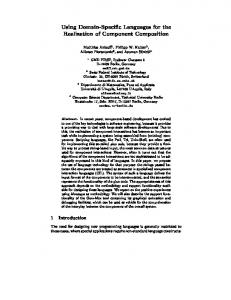
developed the Computerised Activity-Based Stated Preference (CASP) package; the field application that they describe is based on (hypothetically) forcing respondents to travel to work by public transport instead of car, and eliciting their reactions to such a constraint. The Adelaide Travel and Activity Questioner (ATAQ) described in the same paper faces households with parking pricing policies. The studies described in (12) and (13) examine the effects of bus service reductions with pre-determined schedules from which the respondents have to choose. They recognize the need to analyze the behavior of all household members jointly, as well as to consider all activities, not just those that give rise to the journeys affected by the policy measure. Phifer et al. (14) describe an interactive technique called Response to Energy and Activity Constraints on Travel (REACT), which was tested with 12 households in the Albany, New York, area. They recognize that households often counteract travel constraints by modifying non-travel activities, a concept that is picked up in the present study. Lee-Gosselin’s works (15, 16) apply a methodology similar to the HATS, named Car-Use Patterns Interview-Game (CUPIG). 45 households were interviewed about their car use under various fuel shortage scenarios. The studies described in (17) and (18) apply the CHASE (Computerized Household Activity Scheduling Elicitor) framework, which is based on the CUPIG approach, to capture the effects of automobile use reduction scenarios. The three households that were interviewed while testing the approach stated a substantial amount of rescheduling decisions, mainly the adaptation of activity (respectively trip) start and end times as well as mode choice decisions (the latter probably being caused to a large extent by the specific formulation of the experiment). The same software program is used for the study described in (19), where respondents’ planned schedules are recorded in advance and can then be modified on the fly as changes occur in the real world. It is argued that many adaptations to schedules are made at a very short notice, and that the in situ nature of the tool allows capturing those changes very effectively. The approach that is described here is different in that it deals with stated preferences rather than capturing reactions to real changes in a revealed preference framework. Another internet based stated adaptation survey based on congestion pricing scenarios is described in (20). The authors employ an activity based approach, in which various facets of the activity scheduling process can be changed by the respondents. Their survey is different from ours in that a discrete set of options is offered for the adaptation process, rather than the complete restructuring of a reported activity pattern that we aim to capture. Implementation of the Survey Travel Diaries The diary that is administered to the respondents is similar to the multi-day trip based MobiDrive questionnaires that have previously been used in Switzerland (21). An analogous questionnaire was programmed with an internet based interface, for which each participating household receives a user name and password and is assigned a period of five days over which to record their travel. On the web page, the visited locations for a given day are displayed in a table as well as on a map along with color codes for the activity types, in an effort to make the survey more interactive and more attractive to the respondents (Figure 1). Households are given the choice between the internet or a traditional pen-and-paper diary. The software used for the stated adaptation survey, which will be described in the next section, makes use of the same database as
C. Weis, C. Dobler, and K.W. Axhausen
6
the online diary; therefore, data from the pen-and-paper questionnaires must be entered into the web interface before being used in the interviews.
FIGURE 1
Diary web page screen shot (in German).
C. Weis, C. Dobler, and K.W. Axhausen
7
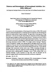
Stated Adaptation Interview Based on the relevant day reported by the respondent and chosen for the stated adaptation interview, the modifications are implemented by the interviewer. Unlike former studies, the scenarios assigned to the respondents in the household interviews are not aimed at determining the effects of specific policies. They are formulated as generally as possible, in the following form: “Imagine your reported trip to [Activity] would take [y] minutes instead of [x]. This may result from the location where the activity was conducted relocating or closing, and you needing to choose a different location.” Travel times for the selected trips (and the return trips, if applicable) are progressively increased by 50, 100 and 200 percent, then decreased by 50 percent, thus creating four scenarios per household. By default, the incurred time losses (or gains) are subtracted from (or added to) the final sojourn at home. The aim is for the household members to state their likely reactions to such a scenario, including the following possibilities: • Choice of a different departure time for certain trips; • Choice of a different travel mode for certain trips; • Changing the order and/or duration of certain activities; • Cancelling certain activities, or adding additional ones; • Switching certain activities between household members; • Combinations of the above. The day for which the household interview is conducted is chosen by the researchers. Ideally, the household members should have conducted a sufficiently large number of activities, so that changes to the schedule become visible and are substantial enough for the household to change its behavior on one of the abovementioned levels. Thus, the day with the largest number of conducted activities is used for the interviews. The assignment of scenarios to the household is carried out using heuristics determining which trip is modified. The following rules are followed: • If at least one household member is employed (or a student), check for commute trips (that is, trips that have either work or education as a purpose). If such trips are present, change their properties; • else, if there are children in the household, check whether accompanying trips to or from the children’s school(s) are present; if so, vary those trips; • else, check whether shopping trips are present, and modify one of them accordingly; • else, modify the longest leisure trip. This procedure ensures that priority is given to mandatory (that is, commute and to a certain extent shopping) trips, which are carried out routinely and for which changing travel conditions represent a larger modification to the scheduling constraints than for leisure trips. The scenarios thus created provide the base for the interactive interviews, where the household members progressively adapt their stated behavior to reach convergence to a schedule that seems satisfying to them. The effects that the scenarios and the stated adaptations have on the respondents’ schedules are directly visible to them. An example day is displayed in the interview software screen shot in Figure 2. Here, the travel time for the bus trip to the work activity (marked by the yellow bar) would be gradually increased from the existing 20 minutes to 30, 45, and 60 minutes, then decreased to 10 minutes, to create the respective scenarios.
C. Weis, C. Dobler, and K.W. Axhausen
FIGURE 2
8
Household interview software screenshot (in German).
Field Work Recruitment Success and Response Rates A total of 2’500 household addresses were acquired from an address retailer, with the requirement that the distribution of household characteristics be representative for the study area (the canton of Zurich). Announcement letters with a brief description of the study are sent to the households. A few days after these introductory letters are dispatched, the interviewers call the potential respondents to establish the households’ willingness to participate in the study and provide them with detailed information on the survey process. At the same time, the potential respondents are informed of an incentive of 20.- Swiss Francs given to each participating person (as of July 2010, 1.- Swiss Franc corresponds to approximately -.94 US dollars). The recruited respondents are assigned the internet or paper questionnaire according to their preference. Key Recruitment and Response Figures (as of July 20th, 2010) Total Online Numbers dialed 2’017 Reached 1’136 Recruited 297 127 Recruitment rate [%] 26.2 Mailed (and reporting period ended) 275 113 Completed diary (households) 134 49 Completed diary (persons) 193 83 Response rate [%] 48.7 43.4
TABLE 1
Paper
171 162 85 110 52.2
C. Weis, C. Dobler, and K.W. Axhausen
9
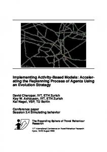
As of July 20th, 2010, phone calls to 2’017 numbers have been carried out, 1’136 of which were answered. Members of 297 households have agreed to participate in the survey, which corresponds to a recruitment rate of 26.2 percent. 171 of the recruited households requested a paper questionnaire, while 127 preferred the internet survey. 85 paper questionnaires have been sent back and found valid (that is, none of the sections were left blank, and the questionnaires provided useable data for the construction of the stated adaptation experiments), and 49 of the invitations to participate in the online survey have yielded useable data. Thus, the response rates for the paper and internet questionnaires are currently at 52.2 and 43.4 percent, respectively. The key figures are displayed in Table 1. As Figure 3 shows, response rates are in line with expectations. They match the experiences with comparable studies at IVT, for which the ex-ante response burden was determined according to the scheme detailed in (22). The methodology assigns weighted scores to question types and sums them up to calculate the overall response burden of a survey. The response rates that are considered here correspond to the COOP4 cooperation rate as defined by the American Association for Public Opinion Research (23). Response rates decrease approximately linearly with response burden, and the present study fits in the corresponding context for surveys with prior recruitment and/or incentive. Response rates from the online and pen-and-paper questionnaires differ slightly, which is in accordance with former experiences made with the two survey modes (24).
100 No prior recruitment, no motivation call No prior recruitment, motivation call
Response rate [%]
80
Prior recruitment / incentive Present study, online Present study, pen-and-paper
60
40
20
0 0
200
400
600
800
1000
1200
Ex-ante assessment of respondent burden FIGURE 3
Response rate in the context of comparable studies.
1400
1600
C. Weis, C. Dobler, and K.W. Axhausen
10
Explorative Analysis of the Sample The first part of Table 2 shows key descriptive figures for the respondent sample in comparison with values for the study area taken from the 2005 Swiss National Household Travel Survey (called Mikrozensus and abbreviated MZ’05; see (25) for a detailed description), a sample which is representative of the Swiss population. Household size and income distributions are given in percent of households, the shares for the other variables in percent of persons in the sample. As can be seen, there is a bias towards the elderly population segment – almost a third of the respondents are over 65 years old, while very few are under the age of 35. The bias becomes even more evident when only the sample of those having responded via the pen-and-paper questionnaire is considered. This may in part be due to the fact that elderly people are more easily reachable by telephone (as they are often retired and thus at home for greater portions of the day than the working population) and, given their larger available time budget, might be more willing to participate in surveys such as the one described here. However, the bias is without any doubt also due to the initial sampling, which was carried out by the address retailer. To counteract the described effect and to attain a more realistic age distribution, the second sample of 1’500 addresses that was acquired (to add to the initial 1’000) had the explicit requirement to contain only individuals aged between 18 and 50. Thus it is hoped that with increasing sample size, the younger age classes will be better represented. Apart from the skewed age distribution, a slight tendency towards rather wealthy households and well-educated respondents can be seen. A high share of respondents own annual transit passes (the Generalabonnement being a flat-rate ticket entitling the owner to free use of public transport in all of Switzerland), as is common for transport surveys in Switzerland. In fact, captive public transport users tend to be more interested in transport policy issues, leading to a higher propensity to participate in the relevant surveys (see (26) for another recent survey where these trends were present). REPORTED TRAVEL BEHAVIOR General Mobility Figures The second part of Table 2 shows a comparison between the share of mobile persons and the average number of trips per day between the online and the pen-and-paper survey as well as the Mikrozensus. As can be seen, reported weekday mobility is at par with the national sample, while trip rates are slightly lower. This may be due to the fact that the Mikrozensus is carried out as a computer assisted telephone interview (CATI), and spans only one day for each respondent. Thus, attrition effects that lead to lower reported mobility as the survey period progresses are expected to be higher in the current study. We hypothesize that a similar effect causes part of the significant drop in reported mobility for Saturdays and Sundays in the online survey.
C. Weis, C. Dobler, and K.W. Axhausen
TABLE 2 Sample Descriptive Statistics and Key Mobility Figures Sample: Sample: Socio-demographic characteristics online paper Variable Value Household size 1 10.4 % 45.6 % 2 35.4 % 43.0 % 3 16.7 % 3.8 % 4+ 37.5 % 7.6 % Household income < 2’000 0.0 % 1.6 % (in Swiss Francs* 2’000 – 4’000 2.4 % 15.9 % per month) 4’000 – 6’000 4.9 % 25.4 % 6’000 – 8’000 29.3 % 22.2 % 8’000 – 10’000 22.0 % 15.9 % > 10’000 41.5 % 19.0 % Gender Male 50.6 % 50.0 % Female 49.4 % 50.0 % Age 18 – 35 10.5 % 3.6 % (in years) 36 – 50 65.8 % 14.5 % 51 – 65 17.1 % 37.3 % > 65 6.6 % 44.6 % Education level Primary or secondary school 6.5 % 8.3 % Vocational school 31.2 % 70.2 % Baccalaureate 5.2 % 9.5 % Higher education 57.1 % 12.0 % Transit pass None 28.6 % 24.1 % Half-fare card 61.0 % 59.2 % Generalabonnement 10.4 % 16.7 % Car availability Always 70.1 % 66.6 % Sometimes 15.6 % 16.7 % Never 14.3 % 16.7 % Sample: Sample: Mobility figures online paper Working days (Monday – Friday) N = 293 N = 394 Share of mobile persons [%] 91.8 % 91.6 % Average number of trips (all persons) 3.57 3.14 Average number of trips (mobiles only) 3.89 3.42 Saturday N = 65 N = 42 Share of mobile persons [%] 70.8 % 92.9 % Average number of trips (all persons) 3.09 3.21 Average number of trips (mobiles only) 4.37 3.46 Sunday N = 48 N = 31 Share of mobile persons [%] 66.7 % 80.6 % Average number of trips (all persons) 2.17 2.26 Average number of trips (mobiles only) 3.25 2.80 * As of July 2010, 1.- Swiss Franc corresponds to approximately -.94 US dollars. ** N is the number of person days in the sample.
11
MZ’05 32.9 % 37.1 % 12.1 % 18 % 3.2 % 17.4 % 26.5 % 20.3 % 13.3 % 19.4 % 48.3 % 51.7 % 28.6 % 29.6 % 23.1 % 18.7 % 11.2 % 60.1 % 7.2 % 19.2 % 50.9 % 39.7 % 9.4 % 72.7 % 20.8 % 6.5 % MZ’05 91.0 % 3.67 4.03 89.4 % 3.26 3.64 79.3 % 2.11 2.66
C. Weis, C. Dobler, and K.W. Axhausen
Modal Share and Trip Purpose Distributions (in Percent) Sample: Sample: Main mode online paper Walk 18.6 21.2 Bicycle 9.5 5.7 Car or motorcycle 52.5 46.0 Public transport 16.4 25.1 Other 3.0 2.0 Sample: Sample: Trip purpose online paper Education 0.9 0.5 Work 19.2 12.1 Shopping / errand 13.2 15.0 Business 2.7 0.7 Leisure 26.7 28.0 Return home 37.3 43.7
12
TABLE 3
MZ’05 28.4 7.0 51.5 11.9 1.2 MZ’05 1.1 16.0 16.0 2.1 25.7 39.1
Modal Split The distribution of the modal shares for the reported trips is displayed in the first part of Table 3, again along with the corresponding figures from the Mikrozensus. Here, significantly less walk trips are being reported, with public transport having a higher modal share than in the national survey. Two reasons can be brought forward for this effect: on the one hand, very short trips (where walking is the preferred mode) tend to be over-represented in the Mikrozensus. On the other hand, the elderly people that are over-represented in our study may more often tend to choose a bus or tram trip over walking, even for short distances. The higher share of transit pass holders also encourages the higher share of public transport. Trip Purposes The trip purpose distribution for the reported trips and its comparison to the figures from the Mikrozensus are shown in the second part of Table 3. Here, representativeness is reached quite exactly. Leisure accounts for about half of the reported out-of-home activities. Education (and, in the paper questionnaire, work) trips are slightly under-represented, which is again due to the age distribution of the sample. REACTIONS TO CHANGES Stated adaptation interviews have so far been conducted with 84 households, accounting for a total of 126 persons. Data from these interviews form the basis for the analyses presented in this section. Changing Travel Conditions As has been mentioned above, the scenarios that are presented to the respondents in the household interviews consist of changing travel times to locations where given activities are conducted. Figure 4 shows the distribution of the changes in total travel times implied by the modifications made in the various scenarios. Changes cover a broad range, reaching from one and a half hours gained to three hours lost travelling.
C. Weis, C. Dobler, and K.W. Axhausen
13
100
Cumulative share [%]
80
60
40
20
0 -90
-60
-30
0
30
60
90
120
150
180
Difference in travel time [min] FIGURE 4
Distribution of implied changes in travel times.
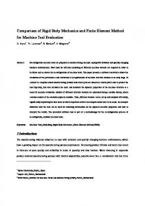
Adaptations in Travel Patterns Removal and Addition of Activities The relationship between the implied changes in travel times and the number of added or removed out-of-home activities is shown in part (a) of Figure 5. The curve was smoothed by calculating a moving average of the underlying data points, of the form: i+n
∑ yj
MAi =
j =i − n
2n + 1
,
where: yi = the value of the variable (difference in number of activities) for the ith observation, the observations being sorted by increasing values of the implied travel time change
n = the number of values around yi that are taken into consideration when computing the moving average MAi ; n was set to 25
C. Weis, C. Dobler, and K.W. Axhausen
14
(a)
Difference in number of trips, moving average [-]
0.1
0 -30
-15
0
15
30
45
60
75
90
-0.1
-0.2
-0.3
Difference in travel time [min] (b)
Average difference in activity duration [-]
10
5
0 > 30
30 - 0
0 - 30
30 - 60
60 - 90
> 90
-5
-10
-15
-20
Difference in travel time [min] FIGURE 5
Changes in activity rates (a) and durations (b) induced by changing travel times.
C. Weis, C. Dobler, and K.W. Axhausen
15
TABLE 4 Summary of Changes in Activity Patterns by Type Type of activity Removals Additions Shorter duration Longer duration Work 4 0 4 0 Education 0 0 0 0 Shopping / errand 2 1 2 1 Business 0 0 0 0 Leisure 5 2 5 2 Home 12 2 35 21 The shown curve serves as a first indicator of how the respondents react to the changes implied in the scenarios. It can be seen that on the one hand, a large majority of the interviewees appear reluctant to make significant modifications to their schedules – a large number of them would not let time losses affect their schedules at all, or at least not to the degree of cancelling activities, leading to the moving averages remaining close to zero. However, as the implied travel times become larger, activities are more likely to be cancelled in order to make up for the time losses. In the same vein, significant time gains tend to increase the number of conducted activities. Moreover, there were only very few cases in which time gains led to activities being removed, or losses to additional ones being conducted; thus, the respondents’ reactions are mostly consistent with the notion that more favorable travel conditions lead to more mobility and vice-versa (that is, that activities can be considered a normal good, for which reduced costs lead to increasing demand). The cases where this assumption does not hold are likely due to secondary effects (such as switching the mode due to a time loss on the initially chosen mode, and using the then resulting time gains to conduct secondary activities). Figure 5 is to be seen as merely diagnostic, while appropriate modeling methods for the data at hand will be applied at a later stage, which will also attempt to consider the abovementioned secondary effects. However, the result can be considered a valuable first test for the consistency of the collected data. Another important aspect concerns the type of activities that are the most likely to be affected by the modifications implied in the survey. The number of cases in which any of the activity types was chosen for addition to or removal from individuals’ schedules is shown in the left-hand part of Table 4. The most frequent activity type to be removed is the sojourn at home. This results from the fact that, as travel conditions worsen, cancelling an intermittent return to the home location (for example, a lunch break between two work activities) is often the most easily conceivable option. Other activity types frequently selected for removal are leisure and, quite surprisingly, work. However, the latter is a side effect of the abovementioned removal of intermittent home trips, leading to separate work activities being merged into a single, and longer, one. The relatively frequent removal and addition of leisure activities is consistent with expectations, as these activities can be planned the most flexibly. Changes in activity durations The right-hand part of Table 4 shows the number of cases in which the durations spent at the respective activity types were shortened or extended. Again, the activity type that is the most frequently affected is the duration spent at home. The general trend of changes in times spent at out-of-home activities induced by changing travel times (averages for six categories) is shown in part (b) of Figure 5. Here again, it becomes obvious that in most cases, the respondents are unwilling to change their activity patterns, as the average activity duration changes are close to zero. There is however a slight
C. Weis, C. Dobler, and K.W. Axhausen
16
tendency towards reducing activity times to compensate at least for part of the travel time losses, particularly when the latter exceed 90 minutes, which appears to be the threshold above which activity rates and durations are significantly affected. Other changes A number of options of changing behavior were indicated by respondents, which could not be directly captured in the interview software. The most frequently mentioned such options are changing either the workplace or the residential location when the commute trip becomes too tedious. The former was considered by 7 respondents, the latter by 4. These remarks were recorded by the interviewers and will be analyzed in future work. CONCLUSION AND OUTLOOK Field work experiences and preliminary results of a stated adaptation survey of travel and activity planning have been presented. Based on reported five day travel diaries, the respondents are faced with changing travel conditions and asked to state their likely reactions to these scenarios on a daily schedule level. The postulated induced travel effect is observed, in that the modifications to the generalized costs of travel affect the respondents’ travel patterns in general, and the number and durations of conducted out-of-home activities in particular. Indicators of the effects have been shown, and are assumed to become clearer as the sample grows. The activities most likely to be re-planned are leisure activities and sojourns at the home location, as is consistent with expectations. Further work will consist of additional survey work, until the target sample of 250 respondents is reached. Based on the collected data, models of activity scheduling will be estimated, which on the one hand should confirm the presence of the abovementioned induced travel effect, and on the other hand will provide the parameters for improved models of activity generation to be implemented in the micro-simulation software MATSim (4). The application will allow the evaluation of aggregate effects of changing generalized costs and of their repercussions on a large scale, as well as the quantitative assessment of total induced demand effects and a comparison to the results from the earlier aggregated models (1, 2). ACKNOWLEDGEMENTS The authors gratefully acknowledge the financial support of the SBT-Fonds administered by the Swiss Association of Transport Engineers (SVI 2004/012) and the advice of the steering committee, chaired by Michel Simon and including René Zbinden, Samuel Waldvogel, Stefan Dasen and Helmut Honermann.
C. Weis, C. Dobler, and K.W. Axhausen
17
REFERENCES 1. Weis, C. Structural Equations Modeling of Travel Behavior Dynamics Using a Pseudo Panel Approach. Presented at 12th International Conference on Travel Behavior Research, Jaipur, 2009. 2. Weis, C. and K.W. Axhausen. Induced Travel Demand: Evidence from a Pseudo Panel Data Based Structural Equations Model. Research in Transportation Economics, Vol. 25, No. 1, 2009, pp. 8-18. 3. Jones, P.M. HATS: A Technique for Investigating Household Decisions. Environment and Planning A, Vol. 11, No. 1, 1979, pp. 59-70. 4. Balmer, M., K. Meister, M. Rieser, K. Nagel, and K.W. Axhausen. Agent-based Simulation of Travel Demand: Structure and Computational Performance of MATSim-T. Presented at 2nd TRB Conference on Innovations in Travel Modeling, Portland, 2008. 5. Louvière, J.J., D.A. Hensher, and J. Swait. Stated Choice Methods: Analysis and Applications. Cambridge University Press, Cambridge, 2000. 6. Arentze, T. and H.J.P. Timmermans. ALBATROSS 2.0: A Learning-based Transportation Oriented Simulation. European Institute of Retailing and Services Studies, Eindhoven, 2005. 7. Jones, P.M. Experience with Household Activity-Travel Simulator (HATS). In Transportation Research Record: Journal of the Transportation Research Board, No. 765, Transportation Research Board of the National Academies, Washington, D.C., 1980, pp. 612. 8. Martin and Voorhees Associates. Reductions in Rural Bus Services: An Independent Assessment of the HATS Technique. Transport Studies Unit, Oxford University, Oxford, 1978. 9. Jones, P.M. and M.C. Dix. HouseholdTtravel in the Woodley-Earley Area: Report of a Pilot Study Using HATS. Transport Studies Unit, Oxford University, Oxford, 1979. 10. Brown, A. and P. Mawson. The HATS Technique: An Urban Application in Basildon New Town. Basildon New Town Development Corporation, Basildon New Town, 1981. 11. Jones, P.M., M. Bradley, and E. Ampt. Forecasting Household Response to Policy Measures Using Computerised, Activity-based Stated Preference Techniques. In International Association for Travel Behavior (eds.) Travel Behavior Research, Avebury, Aldershot, 1989, pp. 41-63. 12. Van Knippenberg-den Brinker C. and M. Clarke. Taking Account of when Passengers Want to Travel. Traffic Engineering and Control, Vol. 25, No. 12, 1984, pp. 602-605. 13. Van Knippenberg-den Brinker, C. and I. Lameijer. Simulation Studies as a Tool for Determining Public Transport Services in Rural Areas. In Jansen, G.R.M., P. Nijkamp, and C.J. Ruijgro (eds.) Transportation and Mobility in an Era of Transition, Elsevier, Amsterdam, 1985, pp. 323-333. 14. Phifer, S.P., A.J. Neveu, and D.T. Hartgen. Family Reactions to Energy Constraints. In Transportation Research Record: Journal of the Transportation Research Board, No. 765,
C. Weis, C. Dobler, and K.W. Axhausen
18
Transportation Research Board of the National Academies, Washington, D.C., 1980, pp. 1216. 15. Lee-Gosselin, M.E.H. In-depth Research on Lifestyle and Household Car Use under Future Conditions in Canada. In International Association for Travel Behavior Research (eds.) Travel Behavior Research. Avebury, Aldershot, 1989, pp. 102-118. 16. Lee-Gosselin, M.E.H. The Dynamics of Car Use Patterns under Different Scenarios: A Gaming Approach. In P.M. Jones (ed.) Developments in Dynamic and Activity-Based Approaches to Travel Analysis, Gower, Aldershot, 1990, pp. 250-271. 17. Doherty, S.T. and M.E.H. Lee-Gosselin. Activity Scheduling Adaptation Experiments under Vehicle Reduction Scenarios. Presented at 9th International Conference on Travel Behavior Research, Gold Coast, 2000. 18. Doherty, S.T., M. Lee-Gosselin, K. Burns and J. Andrey. Household Activity Rescheduling in Response to Automobile Reduction Scenarios. In Transportation Research Record: Journal of the Transportation Research Board, No. 1807, 2002, 174-182. 19. Doherty, S.T. and E.J. Miller. A Computerized Household Activity Scheduling Survey. Transportation, Vol. 27, No. 1, 2000, pp. 75-97. 20. Arentze. T., F. Hofman, and H.J.P. Timmermans. Predicting Multi-faceted Activity-travel Adjustment Strategies in Response to Possible Congestion Pricing Scenarios Using an Internet-based Stated Adaptation Experiment, Transport Policy, Vol. 11, No. 1, 2004, pp. 3141. 21. Löchl, M., K.W. Axhausen, and S. Schönfelder. Analysing Swiss Longitudinal Travel Data. Presented at 5th Swiss Transport Research Conference, Monte Verità, 2005. 22. Axhausen, K.W. and C. Weis. Predicting Response Rate: A Natural Experiment. Survey Practice, Vol. 3, No. 2, 2010. http://surveypractice.org/2010/04/14/predicting-response-rate/. Accessed June 16th, 2010. 23. The American Association for Public Opinion Research. Standard Definitions: Final Dispositions of Case Codes and Outcome Rates for Surveys. http://www.aapor.org/Standard_Definitions1.htm. Accessed Jul. 20, 2010. 24. Weis, C., K.W. Axhausen, A. Frei, T. Haupt, and B. Fell. A comparative study of web- and paper-based travel behaviour surveys. Presented at European Transport Conference, Noordwijkerhout, 2008. 25. Swiss Federal Statistical Office and Swiss Federal Office of Spatial Development. Mobilität in der Schweiz: Ergebnisse des Mikrozensus 2005 zum Verkehrsverhalten. Swiss Federal Statistical Office, Bern, 2005. 26. Weis, C., K.W. Axhausen, R. Schlich, and R. Zbinden. Models of Mode Choice and Mobility Tool Ownership Beyond 2008 Fuel Prices. Presented at 89th Annual Meeting of the Transportation Research Board, Washington, D.C., 2010.