Journal of Transportation Technologies, 2011, 1, 21-29 doi:10.4236/jtts.2011.12004 Published Online April 2011 (http://www.scirp.org/journal/jtts)
Secure Interchange Routing Mark Hartong1, Rajni Goel2, Duminda Wijesekera3 1
Federal Railroad Administration, Washington DC, USA 2 Howard University, Washington DC, USA 3 George Mason University, Fairfax, USA E-mail:
[email protected];
[email protected];
[email protected] Received January 24, 2011; revised February 21, 2011; accepted April 6, 2011
Abstract Locations that connect tracks from different rail-road companies—referred to as interchange points—exchange crew, locomotives, and their associated consists. Because trains have a single degree of freedom in movement, that is, they can only operate along the tracks, any delay occurring at an interchange point causes cascading delays in connecting tracks. In addition, authentication and authorization that is expected to take place at interchanges in PTC controlled train movement may add extra delays due to mutual authentication between two security domains. In this paper we propose a model that can address safety and security concerns and their interrelationships that govern train movement through an interchange point. We show how a profile of safe operations can be computed for operating an interchange point. Keywords: Railroad, Routing, Interchange, Safety, and Security
1. Introduction The primary objective of inter-domain rail operation is to minimize rail traffic delay at interchange points while maintaining safe operating conditions. Delays add to a railroads cost of business and can have a significant impact on the US economy. Techniques used to minimize delays are categorized as tactical (i.e. addresses local scheduling decisions) and strategic (i.e. addresses global scheduling decisions over regions). Taken together they control the end-to-end delays encountered by a trains moving from point A to point B. We address the specific case where points A and B are on different sides of a single rail track that connects two regions belonging to two railroad companies that is commonly referred to as an interchange point. This problem is significant because, if both regions are controlled by the proposed Positive Train Control (PTC) systems, then each side has its own authentication and authorization system that must communicate with the other side to allow an approaching train to go through the interchange point. Our model shows how the two regions can control the movements of trains while maintaining safe inter-train distance and authenticating the crew, and locomotives. The rest of the paper is written as follows. Section 2 discuses delay in the trail environment as it applies to secure interchange operations. Section 3 outlines our proCopyright © 2011 SciRes.
posed model, and the conditions required for safe secure interchange operation. Section 4 takes the conditions for safe secure interchange operations and relates them to underlying physics associated with train operations and communications. Section 5 illustrates the application of our model. Finally Section 6 discusses the limitations of our model, and outlines areas of further research to reduce those limitations.
2. Delays and Delay Modeling Delays impact train operations significantly. For example, in 1997, due to service delays on the Union Pacific (UP) railroad, the State of Texas alone encountered excess costs of over $1.0 billion [1-2]. General delay minimization planning must take into account a whole host of issues such as particular rail lines that are used (line planning), customer service requirements (demand analysis), consist management (allocation of train cars and locomotives), and crew management (distribution and allocation of the train and crew). Each of these has different, and often competing goals. Computing an optimal system wide (strategic) solution requires the ability to schedule the right trains frequently enough to be serviceresponsive to customers, long enough to be cost effective, and spaced so as to minimize transfer time in yards and congestion over the right of way, including interchange JTTs
M. HARTONG
22
points. In this larger planning and scheduling problem, we model the tactical behavior of regarding inter-domain operations. Figure 1 shows three railroads referred to as Railroad A, Railroad B and Railroad C, where we concentrate on the interchange point between Railroad A and Railroad B. As independent entities, each one operates its own trust management system within its own security domain, and consequently has Certificate authorities CA, CB and Dispatcher systems DSA and DSB respectively. We consider the case where trains arriving on Railroad A’s track attempts to enter the interchange point to Railroad B’s side (that is from the bottom right hand side to the bottom left hand track in Figure 1). The trains are named T1, , TX , TX N where X and N are integers. When Railroad A wishes to send Train TX, , TX N to Railroad B’s tracks, two communications may occur. The first is that CA and CB may exchange certificates LX, and DSA and DSB may exchange messages (say MX) in addition to DSA and/or DSB exchanging messages with trains. Figure 1, only illustrate the communications of DSA with CA, TX with DSB and DSA with CA, where other trust management messages may flow. Traffic delays can be a combination of two separate, but interrelated elements. First are delays resulting from the specific physical operating characteristics of the trust management, dispatching and communication systems. The physical operating characteristics include slack time built into the train schedule, traffic congestion, scheduled stops, authorized speeds, location of other trains, on track equipment, maintenance of way work zones, track physical condition, status of signals and communication bandwidth. Although there is an extensive body of work on optimization of network wide routing in general, and railroad networks in particular, such as those described in [3-10], we do not attempt to either develop new, or improve upon existing dispatching and routing methodolo-
Figure 1. Railroad security domains. Copyright © 2011 SciRes.
ET AL.
gies or consider more complex interchange configurations in this paper. The second category of delays arise due to scheduleing at interchange points, where two pre-requisites must be satisfied before movement authority is granted: 1) Lo- comotive and the crew must be authenticated and 2) Tra- ck space must be available in the second domain. Assuming a single unidirectional track with a single siding but no other merging or branching greatly simplifies the optimization of delay at interchanges. Although there are numerous approaches ([11-21]), addressing this configuration these solutions do not consider authentication delays that may occur due to the imposition of a trust management system. Although other more complex track configurations such as using multiple parallel facing or reverse spurs can be built or combinations of facing and reverse spurs can be considered, these cost more money to construct [22]. Having one siding gives the dispatcher much needed room to rearrange the order of trains that proceed to the interchange. For example, the delay of Train TX at the interchange point may be mitigated to some extent by the availability of a siding S. If the train dispatcher for Company A is aware, sufficiently in advance of the arrival of TX , to the interchange point of a potential delay, the dispatcher could direct TX into the siding S, allowing Train TX 1 to proceed along the main line to the interchange point. However, if the siding S is not available, or TX has passed the point in which will allow the dispatcher to direct TX into the siding S, TX will block the following trains from reaching the interchange point. Even if the dispatcher was able to safely divert TX into the siding S, allowing TX 1 to proceed along the mainline to the interchange point, any delay encountered in the process of moving Train TX 1 at the interchange point will delay the following Trains TX 2 through TX N .
3. Cross Domain Operations Our model of the tactical behaviors of Dispatcher A and Dispatcher B relies on the following assumptions: There is a main track and a single siding in domain A and a single main track in domain B. All trains in domain A are of the same length, but may have different priorities for movement. Train movements are from Domain A to Domain B. Dispatcher A (DSA) and B (DSB) have exchanged a session key between each other. Dispatcher A (DSA) has authenticated locomotive TX and the associated engineer EX prior to receiving movement requests. Dispatcher A (DSA) controls the signal whose aspect controls the movement of a train from domain A while Dispatcher B (DSB) controls the signal whose aspect controls the movement of a train into domain JTTs
M. HARTONG
B. For a train to leave domain A and enter domain B, both the Dispatcher A and Dispatcher B have to authorize movement, coordinating the signal aspects. The siding S is of length L and can contain only one train. The main track parallel to the siding may also contain one train. There are up to N trains in the queue awaiting authorization to enter domain B. Requests for authorizations from A to B are in order of increasing distance of trains from interchange point. A train TX is comprised of EX the engineer’s certificate, LX the locomotive certificate, PTCX’, the installed PTC system, VX, the initial train velocity, and DBX the safe stopping (braking) distance. CAA is the certificate authority of domain A. CAB is the certificate authority of domain B. MAX is a movement authority. These conditions reflect actual railroad operating practices. A train TX that has requested entry from one domain to another is prohibited from proceeding into the new domain until the movement authority MAA has been approved by the dispatcher of the new domain. In the event that TX does not receive a response to a request, or the response to a request is delayed, TX proceeds to the limit of its currently granted authority and stops. If TX is already at the limits of the authority, then TX remains halted until the authority to proceed is received. The movement of subsequent trains, Ti for i > (X + 1) and i ≤ N, are rescheduled by the dispatcher in the cur- rent domain by modifying the movement authorities to preclude collisions and overrun of authority limits as necessary. If the dispatcher DSB approves MAX for TX (i.e. the track in domain B is available), dispatcher DSA relays the approved MAX to TX , and TX transitions from domain A to domain B. Dispatcher DSA may then reschedule TX 1 to advance to the block vacated by TX and advance subsequent trains Ti for i ≥ (X + 2). This process is illustrated in Figure 2. This scenario assumes that Dispatcher A is already in possession of the authentication information associated with EX and LX. A train TX that intends to move from domain A to domain B submits the requested movement authority MAX, the engineers certificate EX and the locomotive certificate, LX , (the Access Request in Figure 2) to the Dispatcher A. . Dispatcher A, already being in possession of the necessary certificate information authenticates the requests and forwards it to the Dispatcher in Domain B. Dispatcher B evaluates the feasibility of allowing TX to enter B’s domain. If Dispatcher B approves the movement, he approves MAX and returns it to Dispatcher A. Dispatcher A then Copyright © 2011 SciRes.
ET AL.
23
Figure 2. Movement authority approval.
passes MAX back to TX. TX enters Railroad B’s domain, and Dispatcher A reschedules the movement of TX 1 . Additional scenarios are described in [22]. There are three possible situations that may be encountered by a train TX 1 that is following train TX in Domain A with a single siding. If the main line and siding are clear, TX 1 may take the main or siding and proceed to the interchange point without delay. If the main is clear and the siding is blocked or the main is blocked and the siding is cleared, TX 1 may take the clear track and proceed to the interchange point without delay. If the main and siding are blocked TX 1 may have to wait until the main or siding is clear in order to proceed to the interchange point. In the later situation TX 1 can continue movement to the interchange point if the length of time it takes for TX to receive their authority MAA and move beyond the interchange point is less than the time it takes to stop TX 1 . In the simplest case, where there is a single mainline running between domains A and B, denial of entry of Train TX will require rescheduling of the movement of subsequent trains TX 1 , TX 2 , , TN . In order to preclude a train-to-train collision between the end of Train TX with the head of train TX 1 , train TX 1 must receive notification of the requirement to stop before it proceeds beyond the safe stopping distance BDX 1 . If the movement of train TX 1 is not rescheduled, and train TX 1 does not stop before reaching the location of TX, TX 1 , and TX may collide. If the stopped train TX is released to proceed into the next domain before the train TX 1 , reaches the safe stopping distance, a collision can be avoided. The potential for a collision between train TX 1 and JTTs
24
M. HARTONG
train TX will be affected by the velocity of train TX 1 , the time of release of a stopped train TX, the communication delays associated with information exchanges between CAA and CAB , the dispatcher processing delays DSA and DSB , as well as the PTC system processing times PTCX, and PTC X 1 . The velocity VX 1 of train TX 1 directly affects the safe stopping distance BDX 1 . As VX 1 increases, the safe stopping distance BDX 1 increases, requiring greater separation of trains TX and TX 1 to preclude a collision.”
3.1. Safe Stopping Distance Stopping distances and times for train have been extensively studied (for example [23-26]). Commercial tools to calculate this information using more complex models are exist, most notably the RailSim Train Performance Calculator (TPC) by Systra Consulting, and the Train Operation and Energy Simulator (TOES) by the Association of American Railroads. These estimators reflect a railroads operating philosophy, the type of train (for example passenger or freight), the mass and its distribution of the train, the gradient of the territory the train is operating on at the time of braking, the crews reaction time, and the type of braking (full service, dynamic, or emergency) and the associated deceleration rate induced by the brakes. The braking calculation variables include the types of cars (i.e. tank, box, railrider, etc.), variations in the methods and type of braking (emergency or dynamic, conventional air or electronic pneumatic), track profile (grades and curves), behavior of the locomotive power based on track conditions, details of consist loading and position in the consist of power (head end, middle, or pushing). More approximate estimates for to calculate braking distance exist. For example, [27] is used to predict braking distances for the European Train Control System (ETCS) system. The International Union of Railways (UIC) has promulgated standard 546 [28]. A similar standard is under development by the IEEE [29]. Additional work on braking curves can be found in References [30-35].
3.2. Delay In general, delays of trains proceeding from A to B are prevented when the total delay time associated with certificate authentication and movement authorization is less than the time required to stop the train. If the former is less than the later, then the dispatcher is able to pass the appropriate authorizations to an on-coming train sufficiently in advance of the required safe stopping distance to enable the oncoming train to pass at speed. Prevention of a collision requires that the delays for a train
Copyright © 2011 SciRes.
ET AL.
occupying either a siding or mainline block and the clearance time for the train to clear the block must be less or equal to the time it takes for a following train to brake to a zero velocity. At maximum capacity, the movement of a train from one location to the next requires that the lead train clear the location it is occupying before the trailing train can stop in the location just cleared. This worst-case scenario may occur as a consequence of communication delays compounded by initial authentication of the actors and the first message exchanged. To obtain the total time for a consist to clear, or a consist to stop, the communications overhead times TOH must added to the time to clear of TX and time to stop TX 1 . Provided TX and TX 1 require the same length of time to authenticate (i.e. TOH is a constant for train TX or train TX 1 , the delay TOH cancels out and the delay between individual trains (TX and TX 1 ) remains the same as previously calculated. The assumption that there are no authentication or communications delays is, however, unrealistic. Even in a benign environment, communications disruptions may occur as a consequence of phenomena such as normal atmospheric interference, electromagnetic interference by the AC or DC generators onboard the locomotive, or physical items such as buildings or foliage. To ensure that collisions between a leading train TX and a following train TX 1 do not occur, the authentication and the communications delays TCOMMDELAYX associated with train TX must be less than the communications delays TCOMMDELAYX 1 associated with train TX 1 . If the difference in communications delays is greater than the allowable delay between TX and TX 1 , then the potential exists for the trains to collide. System designs assume that communications disrupttions are likely to occur. To mitigate against this eventuality, not only are the commands retransmitted several times to ensure receipt and acknowledgement, each transmitting and receiving device is equipped with a timer. In the event of a communications disruption that precludes receipt of a valid message, a timer on the device will expire, forcing the device to its most restrictive safe state. This ensures the safety of following trains, albeit with a decrease in system throughput.
4. Physics of Braking and Accelerating Trains The approximate estimate for time to stop assumes constant deceleration in ideal track conditions (i.e. straight (no curvature), level (no up or down grade, and dry). It also assumes the same constant variables (train length, train mass, braking efficiency, target speed, gradient, and distance to target) and that all cars in a particular consist
JTTs
M. HARTONG
are identical and have similar braking characteristics. Likewise, the time to clear a block assumes an identical train operating under the same conditions.
4.1. Time to Clear Tx Assuming constant acceleration from an initial velocity of 0, the time for a train TX stopped at an interchange point (in seconds) where the corresponds to the consist length can be estimated as follows: TC X
2 LX M X 375 FX M X RA
VX
(1)
RA is estimated using the Davis equation. First developed in the mid 1920’s, and modified in the late 1970’s, it provides an estimate of the rolling resistance in pounds per ton [28]. 20 0.01VX RA M X 0.6 X K a VX 2 CarX X nX
(2)
Where MX is the weight of the train TX (tons) LX is the length of the TX (feet) VX is the final velocity of TX (mph) FX is the tractive force of TX locomotives (HP) RA is the drag of the consist when accelerating (lb/ton) wX is the weight per axle per consist car in TX (tons) nX is the number of axles per consist car in TX CarX is the number of cars in the consist in TX Ka is the acceleration drag coefficient Ka = 0.07 The tractive force FX is given by FX N Loco HP E
(3)
4.2. Time to Stop TX + 1 Assuming constant deceleration, the time to stop TS X 1 (i.e. final velocity VX 1 0 ) in seconds is
TS X 1
FX 1 RD
and the drag RD of TX 1 is given by Copyright © 2011 SciRes.
20 0.01VX 1 RD M X 1 0.6 X 1 2 K b VX 1 CarX 1 X 1 nX 1
(5)
Where M X 1 is the mass of the train TX 1 (tons) VX 1 is the initial velocity of TX 1 (mph) FX 1 is the braking force of consist TX 1 RD is the drag of the consist TX 1 when decelerating X 1 is weight per axle per consist car in TX 1 nX 1 is the number of axles per consist car in TX 1 Kb is the braking drag coefficient. Kb = 1.4667 CarX 1 is the number of cars in the consist in TX 1 The braking force FX 1 is given by FX 1 CarX 1 CarWeight X 1
BF BrakeAvail 2000
(6)
Where CarX 1 is the number of cars in the consist TX 1 CarWeight X 1 is the weight of a car in the consist TX 1 (tons) BF is the brake ratio (5%) BrakeAvail is the % operable brakes.
4.3. Consist Delay and Safety Safe operation of the railroad requires that any Train TX 1 not run into the preceding Train TX. For this safety criterion to occur the consist delay between Train TX and TX 1 must satisfy the equation. ConsistDelay TC X TS X 1
(7)
Solving Equation (7) for Consist Delay and substituting Equations (1) and (4) yields the maximum delay that between two trains TX and TX 1 . 0.04583 M X 1 VX 1 ConsistDelay FX 1 RD
Where NLoco is the number of locomotives in TX HP is the Horsepower per locomotive in TX E is the locomotive efficiency %.
0.04583 M X 1 VX 1
25
ET AL.
(4)
(8) 2 LX M X 375 FX M X RA VX
where RA and RB are as defined in Equations (2) and (5). At maximum capacity, the movement of a train from one block to the next requires that the lead train clear the block it is occupying before the trailing train can stop in the block just cleared. This is no different than the case JTTs
26
M. HARTONG
of advancing through the interchange point, the interchange point is simply a special case of a block boundary. Instead of being the boundary between two adjacent blocks in the same domain, it is simply the boundary between two adjacent blocks, one of which is one domain, the other of which is a second domain. If trains TX and TX 1 occupy the main and siding, subsequent trains TX 2 through TX N are blocked from advancing since the trains are restricted to a single degree of motion along the track.
4.4. Communications Delay The physics of train movement, and the impact of communications and authentication delays can be combined into a single equation. The right hand of the inequality is Equation (8), while the left hand side is the time delay due to padding, propagation, and processing delays plus the system response time (SYSRESPONSETIME and SYSPROPAGATION) and the operators response time (OPRESPON- SETIME ). See Equation (9), where M X 1 , MX, VX, VX 1 , LX, LX 1 , LX, LX 1 , RD, RA, FX, and FX + 1 are as previously defined and BSENDERADDRES is the number of bytes of information to identify the sender BRECEIVERADDRESS is the number of bytes of information required to identify the receiver PINFORMATION is the number of bytes of information required to format the information I for transmission CDATA is the number of bytes of information required to control the transmission across the media CPADDING is the number of bytes of information required to format CDATA SDATA is the number of bytes required to convey any security information required for integrity and authenticity SPADDING is the number of bytes required to format SDATA, TR is the communication transmission rate SYSRESPONSETIME is the length of time it takes for the system to process the data once received and change it into information OPRESPONSETIME is the length of time it takes for the operator to respond to a command once received.
ET AL.
SYSPROPAGATION is the propagation delay for the communications medium SYSRESPONSETIME is a function of the performance characteristics of the office subsystem, wayside subsystem, and the onboard subsystem involved in a particular message exchange. OPRESPONSETIME is a function of human factors behavior in receiving, processing, and executing a received command. The advantage of establishing this single safety equation relating all elements is that it allows for the designer to develop risk based performance budgets for the various elements in their design. As long as the overall equation remains true, the designer is free to experiment with various options to achieve the required performance at a particular cost point.
5. An Illustrative Example The behavioral characteristics of the railroad vary greatly depending upon the operating parameters of the trains operating along the railroad. Finding the optimal combination of train parameters that minimizes Consist Delay is a complex problem in operations research. The following example, however, illustrates the use of these equations. For the purposes of this example we will assume TX and TX 1 are identical with properties as follows: Number of Locomotives = 3 Length of locomotive = 100 feet Horsepower per locomotive = 4500 HP Weight per locomotive = 200 tons Locomotive Efficiency = 95% Number of Cars = 100 Weight of a Car = 60 tons Length of a Car = 100 feet Braking Efficiency = 5% Axles per Car = 2 Percent of Brakes Operable = 85% (Minimum operating brakes allowed by Federal Regulations) Train Length = 10300 Feet Communications Bandwidth = 4800 bps All braking is provided by consist cars, locomotive dynamic braking is not considered. More complex scenarios are analyzed in [22].
S Data S Padding BSenderAddress BRe ceiverAddress PInformation CData CPadding SYSRe sponseTime OPResponseTime SYSPr opagation TR 2 LX M X 0.04583 M X 1 VX 1 F R F 375 X M R X 1 D X A V X
(9) Copyright © 2011 SciRes.
JTTs
M. HARTONG
Based on the assumptions in the example, the time required for TX to accelerate and clear, the time for the following TX 1 to decelerate and stop, and the associated delays between the two is shown in Table 1. Negative numbers indicate that a collision can occur. Train TX will not have cleared the interchange point before Train TX 1 arrives. An alternative way to view combinations of leading train clearance time, and following train stopping time is with a radar chart (Figure 3). In this chart, the spokes represent the locomotive speeds, the rings represent clearance times in seconds. As can be seen, for the example configuration, in almost all cases, the time for a leading train to clear the block is less than the time it takes to stop the following train and some delay can occur without adversely impacting subsequent train movements. Changes in locomotive tractive effort and train length also can affect clearance and stopping times, This also is more fully discussed in [22]. The allowable delays previously calculated are based on the physical characteristics of the locomotive and consist as well as the communications bandwidth (4800 bps) available to exchange data. Provided TX and TX 1 reTable 1. Allowable delays V X = V X + 1 . Velocity
Velocity
Clearance
Stop Time
Max Delay
TX
TX+1
Time TX
TX+1
Time
(MPH)
(MPH)
(Seconds)
(Seconds)
(Seconds)
10
10
17.05
11.27
−5.78
20
20
24.48
22.51
−1.97
30
30
30.53
33.69
3.17
40
40
36.00
44.81
8.81
50
50
41.28
55.86
14.58
60
60
46.57
66.82
20.25
Figure 3. Clearance & stopping time. Copyright © 2011 SciRes.
ET AL.
27
quire the same length of time to authenticate (i.e. TOH is a constant for train TX or train TX 1 ), the delay TOH cancels out and the delay between individual trains (TX and TX 1 ) remains the same as previously calculated. With trains TX and TX 1 operating with under condition of nearly simultaneous movement authorities (a method of operation known as moving block and a capability made possible with Positive Train Control (PTC), the required train separation is significantly less than if train movements were not simultaneously. PTC is a wireless communication SCADA system that utilizes a continuous high bandwidth RF data communications network that allows train-to-wayside and wayside-to-train exchange of control and status information. Wayside, office, and trainborne computers process received train status and control data to provide continuous train control [36,37]. With the moving block method of operations, the separation between trains moving at 60 mph can be as low as roughly 3/10th of a mile. When contrasted to the roughly 1.1 miles required by fixed blocks, the traffic density can be increase by roughly a factor of three. This makes significantly better use of the available track resources, and increases system throughput.
6. Conclusions We presented a model for an interchange between two railroad domains governed by interoperating PTC systems for a unidirectional track with a single siding. We showed how to compute the safe conditions by using communication and trust management delays between the two domains. This work provides the signal engineer designing interchanges of some idea of the feasibility of the proposed design. The work needs to be expanded to account for bidirectional train movements on a single track, multiple mainline track with crossovers, multiple sidings, and spurs. Once these more complex tactical routing configurations have be addressed, they can be integrated into strategic models, Establishing these relationships is essential to determine the optimum use of limited resources and continues to remain an open research area. A closed form solution for determining the optimal combination of resources is unlikely, making statistical evaluation of open form solutions necessary and is a subject of future research. There are also a number of implementation related issues that have not been fully addressed in this work. In a operational environment where rail traffic is heavy and close together, the volume of operational and environmental data that must be transmitted may exceed the communications bandwidth. The complete unification of tactical and strategic routing can only be determined in the context of the railroads operaJTTs
M. HARTONG
28
ting environment and the particular implementation mechanisms. Ongoing research in this will provide us with more accurate estimators to support detailed system design and cost evaluation.
7. References [1]
[2]
[3]
[4]
[5]
B. Weinstein and T. Clower, “The Impact of the Union Pacific Service Disruptions on the Texas and National Economies: An Unfinished Story,” Railroad Commission of Texas, Austin, February 1998. “Joint Petition for Service Order, STB Service Order No. 1518,” Surface Transportation Board, Washington DC, 31 October 1997. Transportation Research Board of the National Academies, “US Railroad Efficiency: A Brief Economic Overview,” Proceedings of the Workshop on Research to Enhance Rail Network Performance, Washington DC, 5-6 April 2006, pp. 63-71. M. Dessouky, Q. Lu, J. Zhao and R. Leachman, “An Exact Solution Procedure to Determine the Optimal Dispatching Times for Complex Rail Networks,” IEE Transactions, Vol. 32, No. 2, 2006, pp. 141-152. M. Khan, D. Zhang, M. Jun and J. Zhu, “An Intelligent Search Technique to Train Scheduling Problem Based on Genetic Algorithms,” Proceedings of the 2006 International Conference on Emerging Technologies, Perhwar, 13-14 November 2006, pp. 593-598. doi:10.1109/ICET.2006.335970
[6]
A. Tazoniero, R. Gonclaves and F. Gomide, “Decision Making Strategies for Real Time Train Dispatch and Control Analysis and Design of Intelligent Systems Using Soft Computing Techniques,” Advances in Soft Computing, Springer, Vol. 41, 2007, pp. 193-204.
[7]
F. Li, Z. Gao, K. Li and L. Yang, “Efficient Scheduling of Railway Traffic Based on Global Information of Train,” Transportation Research, Part B: Methodological, Vol. 42, No. 10, 2008, pp. 1008-1030.
[8]
[9]
M. Penicka, “Formal Approach to Railway Applications,” Formal Methods and Hybrid Real Time Systems, Lecture Notes in Computer Science, Springer, Vol. 4700, 2007, pp. 504-520. doi:10.1007/978-3-540-75221-9_24 M. Carey and I. Crawford, “Scheduling Trains on a Network of Busy Complex Stations,” Transportation Research, Part B: Methodological, Vol. 41, No. 2, 2007, pp. 159-178.
ET AL. Scheduling at Industrial In-Plant Railroads,” Transportation Science, Vol. 37, No. 2, 2003, pp. 183-197. [13] A. E. Kozan and A. Higgins, “Modeling Train Delays in Urban Networks,” Transportation Science, Vol. 32, No.4, 1998, pp. 346-357. [14] Q. Lu, M. Dessouky and R. Leachman, “Modeling Train Movements through Complex Rail Networks,” ACM Transactions on Modeling and Computer Simulations (TOMACS), Vol. 14, No. 1, 2004, pp. 48-75. [15] D. Parkes and L. Ungar, “An Auction Based Method For Decentralized Train Scheduling,” Proceedings of the 5th International Conference on Autonomous Agents, Montreal, 28 May-1 June 2001, pp. 43-50. [16] J. Lee, K. Sheng and J. Guo, “Fast and Reliable Algorithm for Railway Train Routing,” Proceedings of the IEEE Region 10 Conference on Computers, Communications, Control Engineering, Beijing, 19-21 October 1993, pp. 652-655. [17] D. Ariano, M. Pranzo and I. Hansen, “Conflict Resolution and Train Speed Coordination for Solving Time Table Perturbations,” IEEE Transactions on Intelligent Transportation Systems, Vol. 8, No. 4, 2007, pp. 208-222. [18] T. Ho, J. Norton and C. Goodman, “Optimal Traffic Control at Railway Junctions,” IEE Proceedings of Electric Power Applications, Vol. 144, No. 2, 1997, pp. 140-148. [19] M. Lewellen and K. Tumay, “Network Simulation of a Major Railroad,” Proceedings of the 30th Winter Simulations Conference, Washington DC, 13-16 December 1998, pp. 1133-1138. [20] S. Graff and P. Shenkin, “A Computer Simulation of a Multiple Track Rail Network,” Sixth International Conference on Mathematical Modeling, St. Louis, 4-7 August 1987, pp. 472-475. [21] T. Ho and T. Yeung, “Railway Junction Traffic Control by Heuristic Methods,” IEE Proceedings of Electric Power Applications, Vol. 148, No. 1, 2001, pp. 771-772. [22] M. Hartong, “Secure Communications Based Train Control Operations,” Doctoral Dissertation, George Mason University, Fairfax, May 2009. [23] D. Barney, D. Haley and G. Nkandros, “Calculating Train Braking Distances,” Proceedings of the 6th Australian Workshop on Safety Critical Systems and Software, Brisbane, 6 July 2001, pp. 23-29. [24] “IEEE Std. 1474.1-2004,” IEEE Standard for Communications-Based Train Control, Appendix D, IEEE, Piscataway, 2004.
[10] J. Tornquist, “Computer-Based Decision Support for Railway Traffic Scheduling and Dispatching, A Review of Models,” Proceedings of the 5th Workshop on Algorithmic Methods and Models for Optimization of Railways, Palma de Mallorca, 14 September 2005.
[25] T. M. Malvezzi, P. Presciani, B. Allotta and P. Toni, “Probabilistic Analysis of Braking Performance In Railways,” Proceedings of the Institution of Mechanical Engineers, Part F: Journal of Rail and Rapid Transit, Vol. 217, No. 3, 2003, pp. 149-165.
[11] L. Anderegg, I. Stephan, E. Gantenbein and I Stature, “Train Routing Algorithms: Concepts, Design Choices, and Practical Considerations,” Proceedings of the 5th Workshop on Algorithm Engineering and Experiments, Baltimore, 11 January 2003, pp. 106-118.
[26] B. Vincze and G. Tarmai, “Development and Analysis of Train Brake Curve Calculation Methods with Complex Simulation,” Proceedings of International Exhibition of Electrical Equipment for Power Engineering, Electrical Engineering, Electronics, Energy and Resource-Saving Technologies, Household Electric Appliances, Zilina, 23-
[12] M. Lubbecke and U. Zimmermann, “Engine Routing and Copyright © 2011 SciRes.
JTTs
M. HARTONG 24 May 2006, pp. 199-211. [27] B. Friman, “An Algorithm for Braking Curve Calculations in ERTMS Train Protection Systems,” COMPRAIL 2006 10th International Conference on Computer System Design and Operation in the Railway and Other Transit Systems, Prague, 10-12 July 2006, pp. 421-430. [28] “BS 05/19984709 DC (UIC-546) EN 15179. Railway Applications Braking. Requirements for the Brake System of Passenger Coaches,” British Standards Institution, London, March 2005. [29] “Draft Guide for the Calculation of Braking Distances for Rail Transit Vehicles, IEEE P1698/D1.3,” IEEE, Piscataway, 2008. [30] F. Yan and T. Tang, “Formal Modeling and Verification of Real-time Concurrent Systems,” Proceedings of the IEEE International Conference on Vehicular Electronics and Safety, ICVES 2007, Beijing, 13-15 December 2007, pp. 1-6. [31] E. Khmelnitsky, “On an Optimal Control Problem of Train Operation,” IEEE Transactions on Automatic Control, Vol. 45, No. 7, 2000. [32] L. Y. Zhang, P. Li, L. M. Jia and F. Y. Yang, “Study on the Simulation for Train Operation Adjustment under Moving Block,” Proceedings of the 2005 Intelligent
Copyright © 2011 SciRes.
ET AL.
29
Transportation Systems,” Vienna, 13-16 September 2005, pp. 351-356. doi:10.1109/ITSC.2005.1520153 [33] H. Takeuchi, C. Goodman and S. Sone, “Moving Block Signaling Dynamics: Performance Measures and Re-starting Queued Electric Trains,” IEE Proceedings Electric Power Applications, Vol. 150, No. 4, 2003, pp. 483-492. [34] H. Krueger, E. Vaillancourt, A. Drummie, S. Vucko and J. Bekavac, “Simulation in the Railroad Environment,” Proceedings of the 2000 Winter Simulation Conference, Orlando, 10-13 December 2000, pp. 1048-1055. [35] W. Rudderham, “Longitudinal Control System of the Intermediate Capacity Transit System,” Proceedings of the 33rd IEEE Vehicular Technology Conference, Toronto, 25-27 May 1983, pp. 183-190. doi:10.1109/VTC.1983.1623131 [36] “Railroad Communications and Train Control, Report to Congress,” Federal Railroad Administration, Washington DC, July 1994 [37] “Report of the Railroad Safety Advisory Committee to the Federal Railroad Administrator, Implementation of Positive Train Control Systems,” Federal Railroad Administration, Washington DC, August 1999.
JTTs