Simulating Water-Quality Trends in Public-Supply Wells in Transient Flow Systems by J. Jeffrey Starn1 , Christopher T. Green2 , Stephen R. Hinkle3 , Amvrossios C. Bagtzoglou4 , and Bernard J. Stolp5
Abstract Models need not be complex to be useful. An existing groundwater-flow model of Salt Lake Valley, Utah, was adapted for use with convolution-based advective particle tracking to explain broad spatial trends in dissolved solids. This model supports the hypothesis that water produced from wells is increasingly younger with higher proportions of surface sources as pumping changes in the basin over time. At individual wells, however, predicting specific water-quality changes remains challenging. The influence of pumping-induced transient groundwater flow on changes in mean age and source areas is significant. Mean age and source areas were mapped across the model domain to extend the results from observation wells to the entire aquifer to see where changes in concentrations of dissolved solids are expected to occur. The timing of these changes depends on accurate estimates of groundwater velocity. Calibration to tritium concentrations was used to estimate effective porosity and improve correlation between source area changes, age changes, and measured dissolved solids trends. Uncertainty in the model is due in part to spatial and temporal variations in tracer inputs, estimated tracer transport parameters, and in pumping stresses at sampling points. For tracers such as tritium, the presence of two-limbed input curves can be problematic because a single concentration can be associated with multiple disparate travel times. These shortcomings can be ameliorated by adding hydrologic and geologic detail to the model and by adding additional calibration data. However, the Salt Lake Valley model is useful even without such small-scale detail.
Introduction Interpreting water-quality trends in hydrologically complex and (or) transient groundwater-flow systems is challenging. Groundwater modeling can help unravel complex interaction among variables by providing a framework for that interaction that is consistent with the physics of groundwater flow. In particular, a model can be used to compute spatial and time-series quantities that can be used to explain measured water-quality changes. 1
Corresponding author: U.S. Geological Survey, 101 Pitkin Street, East Hartford, CT 06108;
[email protected] 2 U.S. Geological Survey, Bldg. 15 McKelvey Building, 345 Middlefield Rd. 496, Menlo Park, CA 94025;
[email protected] 3 U.S. Geological Survey, 2130 SW 5th Ave., Portland, OR 97201;
[email protected] 4 Department of Civil and Environmental Engineering, University of Connecticut, 261 Glenbrook Rd., Unit 3037, Storrs, CT 06269;
[email protected] 5 U.S. Geological Survey, 2329 W. Orton Circle, West Valley City, UT 84119;
[email protected] Received July 2013, accepted April 2014. Published 2014. This article is a U.S. Government work and is in the public domain in the USA. Groundwater published by Wiley Periodicals, Inc. on behalf of National Ground Water Association. This is an open access article under the terms of the Creative Commons Attribution-NonCommercial License, which permits use, distribution and reproduction in any medium, provided the original work is properly cited and is not used for commercial purposes. doi: 10.1111/gwat.12230
NGWA.org
The purpose of this study is to (1) evaluate the use of an existing transient groundwater-flow model to answer water-quality questions, (2) develop and test modelderived time-dependent variables in relation to measured water-quality trends, and (3) evaluate the usefulness of tracer calibration data for the purpose of explaining trends. The approach used in this study is to adapt an existing groundwater-flow model for advective transport simulation by adjusting effective porosity to match tritium concentrations in samples from wells. The model is then used to estimate changes over time in groundwater age and source area and to relate these changes to measured trends in dissolved solids concentrations in Salt Lake Valley, Utah. This study draws on previous work by the authors and will help guide future transport modeling of regionalscale groundwater-quality trends in transient flow systems. Recent editorials/articles by Konikow (2011), Voss (2011a), and Voss (2011b) raise questions about appropriate complexity of transport models, including the role of macrodispersion (especially at the regional scale), meaningful values of effective porosity, and simultaneous calibration of flow and transport properties. Macrodispersion is a primary transport mechanism in groundwater; however, several studies of regional-scale transport have used advection-only to provide a first-order estimate of solute concentrations. For example, Sanford (2011) and Green et al. (2010) simulated groundwater age using only advection. Simulations of advective groundwater transport
Vol. 52, Groundwater–Focus Issue 2014 (pages 53–62)
53
In the Salt Lake Valley, Utah (Figure 1), the basin-fill aquifer is bounded by mountains to the east, south, and west and by Great Salt Lake to the north. Quaternary-age basin fill consists of unconsolidated to semi-consolidated sediments deposited in climate-driven cycles of lacustrine, deltaic, and alluvial environments (Stolp 2007). Sediments average 600 m thick in interbeds of clay, silt, sand, and gravel and lenses of sand and gravel. Sediments originated from the adjacent mountains and are generally coarser and less well sorted near the valley wall and finer near the center of the valley. Discontinuous fine-grained layers confine groundwater in the central part of the basin. These layers are not present near the basin edges, and recharge occurs there from losing stream reaches, infiltrating precipitation, and flow through fractured consolidated 112°0'0"W
111°50'0"W
Sa Gr lt eat La ke
112°10'0"W
Idaho Wyoming Nevada
Utah
Colorado
40°50'0"N
Jordan River
Salt Lake City
Magna
Big C
otto
n wo
40°40'0"N
od C
re e k
n to oo w
West Jordan
ot d C re ek
J.J. Starn et al. Groundwater 52, Focus Issue: 53–62
Salt Lake Valley Geology and Water Quality
C
54
fundamentally important characteristic of the groundwater system in Salt Lake Valley. Models are built for specific purposes, and using a model for a purpose other than for which it was intended can lead to misleading results. It is a significant question whether groundwater models built to answer questions about water levels and flow rates can be used to explain possible causes of water-quality trends. The model used in this study provides an example; it was created to answer questions about water levels and flow rates in Salt Lake Valley, Utah (Lambert 1995).
e ttl Li
have been successfully used to interpret trends of solute concentrations (Kauffman et al. 2001; McMahon et al. 2008) and assess groundwater age (Wellman et al. 2012) in steady flow. One reason these efforts were successful is that groundwater at receptors such as streams or wells at the regional scale integrates a wide distribution of flow paths, source areas, and groundwater ages. These successes suggest that simulation of advection without consideration of macrodispersion would adequately represent large spatial scale transport in this regional system. Effective porosity, which converts inter-cell flux to velocity (Konikow 2011), is required to adapt a groundwater-flow model for transport simulation. It accounts for the fact that transport does not occur evenly throughout a cross section of flow and does not include pore spaces that are not connected. For this reason prior estimates of effective porosity vary widely (Konikow 2011) and often are not available. In this study, effective porosity is adjusted as part of the calibration process so that simulated tritium concentrations match tritium concentrations measured in samples from pumping wells. Advective transport models have been calibrated to tritium/helium age dates (Reilly et al. 1994; Sheets et al. 1998; Murphy et al. 2011); however, fewer studies have relied solely on tritium concentrations. Ideally all calibration data (hydraulic heads, streamflow, and tritium concentrations) could be simulated by a single flow and transport model and parameters of the flow model (e.g., hydraulic conductivity and storage coefficient) adjusted simultaneously with effective porosity. However, as Voss (2011a, 2011b) points out, this may not be possible because of disparate transport processes—heads change instantaneously and uniformly throughout an aquifer, whereas mass changes discretely and nonuniformly through permeable pathways in an aquifer. In this study, the flow model is not modified; groundwater velocity is calibrated by adjustment of effective porosity. Groundwater-flow systems are never really in steady state, and there are relatively few studies that consider transient flow in analyzing water-quality trends (Furlong et al. 2011). In transient flow, age distributions become time dependent (Manning et al. 2012) and the system’s response to solute input also depends on time. Time-dependent source areas (Rock and Kupfersberger 2002; Masterson et al. 2004) possibly contribute different solutes to groundwater, resulting in a complex mixture of water at the receptor (Starn and Brown 2007). Simulation of transient flow can be used to unravel these processes by showing possible changes in source areas and groundwater ages. Short-term recharge variations cause transient flow, but the timescale of groundwater flow often is much longer, in which case the effect is minimal over time (Reilly and Pollock 1996). However, long-term recharge or discharge variations (longer than the timescale of groundwater flow) can lead to significant long-term changes in water quality. Transient flow caused by pumping variations is simulated in this study as a
Draper
40°30'0"N
0
8 Miles
Water quality from Thiros and Spangler 2010
Figure 1. Salt Lake Valley, Utah. Solid black line is extent of active model grid. Tan area is water ≤500 mg/L dissolved solids in 1998.
NGWA.org
rock in the adjacent mountains. Recharge through the confining layers from an overlying shallow unconfined aquifer also occurs, but to a lesser degree. The simulated aquifer includes tertiary-age semi-consolidated sediments at its base where they are permeable enough to yield water to wells (Stolp 2007). Groundwater flow is from the recharge areas primarily to the Jordan River in the center of the valley (Figure 1) and to pumping wells. Groundwater from wells supplied about 29% of the water used for public supply in the basin in 2005 (Thiros and Spangler 2010). While most of the groundwater pumped is used for drinking, some is used for agricultural and industrial purposes (Burden 2009). Groundwater also discharges through springs and evapotranspiration. Thiros and Spangler (2010) documented increasing dissolved solids in wells over a wide area using long-term water-quality records from the 1930s to the 2000s. In the Salt Lake Valley aquifer, a plume of water containing less than 500 mg/L dissolved solids is surrounded by groundwater of higher dissolved solids concentrations (Figure 1). Note that here “plume” refers to water that is of better quality for drinking, not lower as the term is usually used. Sources of dissolved solids include mineral dissolution from aquifer sediments, infiltration of de-icing chemicals, and concentration by evaporation in surfacewater sources to the Jordan River. Some parts of the aquifer contain older water that has been in contact with aquifer minerals for centuries or millennia, resulting in high-dissolved solids concentrations (Thiros and Spangler 2010). Carbon-14 and Helium-4 data support very old ages in some wells in Salt Lake Valley (Stephen Hinkle USGS 2012, unpublished data). Dissolved solids from mineral dissolution occur in several broad categories of water, including water containing: calcium, bicarbonate, and sulfate from dissolution of shale minerals, sulfate from oxidation of sulfide minerals; and sodium and chloride from desiccated paleolakes. Dissolved solids in water from other wells, however, have fluctuated within a small range. The plume appears to be associated with water coming from terrain underlain by relatively erosion-resistant rock in the adjoining mountains. Sources of water to these wells probably include recharge from snowmelt and subsurface inflow from adjacent mountain block areas. Population in the valley steadily increased from the 1930s to more than 1 million people in 2011. Although pumping at individual wells has increased or decreased over time, total withdrawals from the aquifer leveled off after about 1997. During the period of population increase, many wells for which there are long-term data had changes in dissolved solids concentration. Changes in dissolved solids concentrations over time can be related to changing human activities such as increased use of deicing chemicals and changes in the location and magnitude of groundwater withdrawals from wells. Groundwater withdrawals can induce flow from new source areas by enhancing downward flow from areas affected by recent anthropogenic activity or horizontal flow from areas affected largely by natural mineral processes. NGWA.org
Groundwater withdrawals and changes in storage were relatively constant from 1964 to 1968, and a steady-state model for that time period was manually calibrated to measured water levels, groundwater flow to the Jordan River, and vertical hydraulic gradients in the aquifer (Lambert 1995). The steady-state simulation was used as the initial condition for a transient simulation in which recharge and pumping rates were varied at their estimated annual rates from 1969 to 1991. The transient model was manually calibrated to measured water-level changes and groundwater flow to the Jordan River (Lambert 1995). Lambert (1996) extended the original simulation for part of the modeled area to include the time period 1935 to 1964. Total water use and public-supply annual withdrawals were relatively constant from 1997 to 2009 (Burden 2009), although the withdrawal at individual wells may have changed, causing local water-level fluctuations. Stolp (2007) updated groundwater withdrawals and recharge in the model to reflect average 1997 to 2001 conditions. The models constructed by Lambert (1995, 1996) and modified by Stolp (2007) cover 1,152 km2 of the Salt Lake Valley. The model grid cells are 563.27 m on each side in 94 rows and 62 columns. The aquifer is divided into seven layers; the top two layers represent a shallow unconfined aquifer and an underlying confining unit in the center of the valley. The thickness of the two layers is variable. Layers 3 through 7 represent the principal aquifer and are 46, 46, 46, 61 m, and greater than or equal to 61 m thick, respectively. Layer 7 is a maximum of 460 m thick in the deepest parts of the basin. Boundary conditions include recharge from precipitation, losing streams, and the mountain block and discharge through pumping wells, gaining stream reaches, and evapotranspiration. The base of the aquifer is a zero-flow boundary. More details on model properties, boundaries, and calibration are given by Lambert (1995, 1996) and Stolp (2007). The original model by Stolp (2007) was modified from Lambert (1995, 1996) for MODFLOW-2000. For this project, the model was modified for use with MODFLOW-NWT (Niswonger et al. 2011) which necessitated changing from the original block-centered flow package to the layer property flow package (Harbaugh 2005). Also, for this work, the multi-node well package for MODFLOW (Konikow et al. 2009) was used to better simulate the public-supply wells. No other changes were made to the model. The differences between the flow budgets in all stress periods between the original model and the modified model were very small and were considered negligible.
Approach Groundwater age distributions at observation wells were simulated using transient particle tracking (MODPATH; Pollock 2012) rather than grid-based methods (e.g., MT3DMS; Zheng and Wang 1999) for efficiency and to limit numerical dispersion. Age distributions were transformed to tritium concentration breakthrough J.J. Starn et al. Groundwater 52, Focus Issue: 53–62
55
curves (BTCs) using convolution-based particle tracking (CBPT; Robinson et al. 2010). Convolution transforms the impulse response of a system to a response of the system that reflects time-varying input (Małoszewski and Zuber 1982). Flow-model grid cells were relatively large, and an analytical equation was used to compute velocity near pumping wells as described by Zheng (1994) and adapted for use with MODPATH by Starn et al. (2012, 2013). Although CBPT is only applicable to steady-state flow systems, recent work extends CBPT to time-varying flow by assuming steady flow over small time intervals (Srinivasan et al. 2011; Starn et al. 2013). Calibration of the Salt Lake Valley flow model is well documented (Lambert 1995, 1996; Stolp 2007), and no parameters of that model were changed in order to maintain the integrity of its calibration. Also, adjusting only porosity avoids difficulty with numerical instability in the flow model caused by the addition of correlated parameters (porosity and hydraulic conductivity). To adapt the groundwater-flow model for waterquality simulation, the effective porosity is required, which converts the inter-cell flux calculated by the model to velocity. Effective porosity was adjusted using the inverse modeling program PEST++ (Welter et al. 2012) to minimize the sum of squared differences between CBPT simulated equivalent concentration and tritium concentrations measured in samples from pumping wells. In this study, tritium concentrations and tritium/helium apparent ages were available for model calibration, although the ages were not used in the final calibration.
Tracer Concentration Data Tritium concentrations from 80 wells are available for model calibration, mainly in the area where dissolved solids changes have been measured. Some of the wells have been sampled multiple times for a total of 122 concentrations; 61 of these values are paired with a tritium/helium apparent age date. The timescale of tritium persistence in this aquifer system (decades) is comparable to the temporal scale of changes in dissolved concentrations; therefore, calibration to these data should serve to decrease uncertainty in the model. Most of the tritium data are in the USGS National Water Information System database (http://waterdata.usgs.gov/ut/nwis/qw/). Additional data are contained in the papers by Manning (2002), Thiros (2003), and from USGS sites reported by University of Utah and Lamont-Doherty Earth Observatory. Tritium/helium apparent ages are available from the papers by Thiros (2003) and Thiros and Manning (2004).
TU (tritium unit) was used as the value of pre-bomb and post-2000 tritium concentrations, as estimated by Thatcher (1962) for the central United States. This tritium input function is the estimated input to land surface, not to the water table. Analysis by Manning et al. (2005) provides evidence for generally negligible tritium residence time ( 49 - 250 40°50'0"N
> 250 - 500 > 500 - 1386
40°40'0"N
E D
40°30'0"N
0
8 Miles
Water quality from Thiros and Spangler 2010
Figure 4. Range of changes in dissolved solids in mg/L and extent of water with dissolved solids ≤500 mg/L. Ranges are depicted for wells for which time series were available. Additional wells were sampled to determine extent in 1964 (tan area) and 1998 (enclosed by solid black lines) of water with dissolved solids ≤500 mg/L.
the sum-of-squared errors by about 50%. Calibration also was attempted with data sets that included the tritium/helium age dates. Including ages in the calibration did not alleviate nonuniqueness, and ages were not used in the final calibration. Tracer age only corresponds to mean particle age if the flow system is approximated by piston flow, and in a transient flow system complicated by pumping, this was not deemed likely. J.J. Starn et al. Groundwater 52, Focus Issue: 53–62
57
(B)
(A) 1950 1965 1980 1995 2010
(C)
Well D
(D)
Water quality from Thiros and Spangler 2010
Figure 5. Results of simulation for Well D (water quality shown in Figure 4). Panel A, source area of particles released from well in year indicated by color; B, simulated mean age, measured dissolved solids dashed line with circles; C, source of water (MBR is mountain block recharge); D, layer contributions.
Although most simulated BTCs fit the relative magnitude (Figure 3A) and trend of measured tritium (Figure 3C), the fit at some wells was not good (Figure 3B). Local variations in hydraulic properties and the coarseness of simulated pumping history (as in Figure 3B) were probably the largest contributors to poor fit. Existing porosity estimates for the east side of the valley (Freethey et al. 1994) show an increase from the east edge of the valley toward the Jordan River with zones of higher porosity beneath Big and Little Cottonwood Creeks. The estimated effective porosity distribution from using pilot points was similar, although the magnitudes were relatively low, ranging from 0.03 to 0.15. The smoothness criteria prevented a wider range of values. This range probably was lower than Freethey et al. (1994) estimates because the degree of connectedness of porosity was less than expected and because it accommodates lack of small-scale detail in the flow model.
Simulated Factors Related to Dissolved Solids Trends The area of the Salt Lake Valley aquifer containing water less than 500 mg/L dissolved solids decreased from 1964 to 1998, and the concentration of dissolved solids in many long-term observation wells increased over the same period (Thiros and Spangler 2010). The largest increases are along the southern margin of an area surrounding Big and Little Cottonwood Creeks (shaded area in Figure 4). 58
J.J. Starn et al. Groundwater 52, Focus Issue: 53–62
One hypothesis is that increased pumping has increased the proportion of water recharged from surface sources (as opposed to mountain block recharge) in these wells. Three model-derived explanatory factors that can be used to test the hypothesis were developed using the calibrated model. The first factor was the fraction of each water source contributing to a well over time created by tagging reverse-tracked particles starting in a well with their ending locations (corresponding to the sourcewater area). The second factor was the fraction of water supplied to the well from each model layer calculated by the Multi-Node Well package (Konikow et al. 2009) in MODFLOW. The third factor was the mean simulated age created by taking the mean age of particles reverse-tracked from the well. The wells with the highest range of increased dissolved solids all had simulated sources area that changed over time with respect to the plume location (for example, Well D in Figure 5A). Pumping apparently increased in well D or in a nearby well(s) around 1980. At the same time, the mean age decreased (Figure 5B), the proportion of water coming from surface sources increased (Figure 5C), and water traveled to the well through shallower model layers (Figure 5D). Source areas in the center of the plume (Well E in Figure 6A) changed with time but remained within the plume. The initial age of water in this source area was much younger than in well D (Figure 6B) and also decreased as the proportion of surface sources increased (Figure 6C). NGWA.org
(A)
1950
(B)
1965 1980 1995 2010
(C)
Well E
(D)
Water quality from Thiros and Spangler 2010
Figure 6. Results of simulation for Well E (water quality shown in Figure 4). (A) Source area of particles released from well in year indicated by color; (B) simulated mean age, measured dissolved solids dashed line with circles; (C) source of water (MBR is mountain block recharge); (D) layer contributions.
2020
1950
0
4
8 Miles
Water quality from Thiros and Spangler 2010 Precipitation
Canals
Mountain block
Jordan River
1998 TDS < 500 mg/l
Figure 7. Simulated change in sources of water to model layer 3 from 1950 to 2020. Layer 3 is at typical depth for public water supply.
NGWA.org
J.J. Starn et al. Groundwater 52, Focus Issue: 53–62
59
2020
1950
0
4
8 Miles
Water quality from Thiros and Spangler 2010 Mean age of water in years 0.20 - 20
>20 - 60
>60 - 500
>500
1998 TDS < 500 mg/l
Figure 8. Simulated change in mean age of water to model layer 3 from 1950 to 2020. Layer 3 is at typical depth for public water supply.
Broad spatial patterns of sources and mean ages correspond predictably to the measured spatial shifts in dissolved solids concentration. Changes in source area and mean age can be mapped by placing particles at the center of each model cell at specific times (1950 and 2020 shown in the Figures 7 and 8) and reverse tracking them to their source. The broad spatial trend is for less water from mountain block recharge and more water from leaking canals and river reaches (Figure 7). In the center of the model area, more water is coming from canal and river leakage; along the model edges, less water is coming from mountain sources over time. Similarly, the mean age (Figure 8) in model layer 3 decreases over time in the southern two-thirds of the model area, consistent with a downward shift of recently recharged water originating from surface sources.
Conclusions Models need not be complex to be useful. A complex model in this sense would be one that simulated macrodispersion, chemical reactions in the aquifer, and detailed aquifer heterogeneity, which this model does not do. Although prediction of solute concentration trends at 60
J.J. Starn et al. Groundwater 52, Focus Issue: 53–62
individual wells in complex systems remains a challenging problem, this work shows that an existing flow model of Salt Lake Valley, Utah, adapted for transport simulation was useful in explaining measured dissolved solids trends. At individual wells, the source fraction, mean age, and depth (model layer) change in concert with dissolved solids but not always in an easily predictable way. 1. The model provided a physically consistent framework of model and data that support the hypothesis that water produced by wells is increasingly younger with higher proportions from surface sources as a result of pumping. The most useful predictive variables for changes in dissolved solids are the changes in source area location and mean age. These variables change over time, and transient changes in the flow system must be considered in order to explain trends. An accurate estimation of velocity (through inverse modeling of effective porosity in this case) is important for assessing the timing of those changes. 2. Changes in mean age and source areas can be mapped across the model domain to extend the results at wells to the entire aquifer area to see where changes are expected to occur. However, constituents such as NGWA.org
dissolved solids are affected by many geochemical processes. To make full use of model-derived factors, one must incorporate how recharge solute chemistry changes at the land surface and how rock-water interactions alter the composition of groundwater. 3. Calibration to tracer data can improve correlation between model-derived factors and measured waterquality trends. However, effective porosity estimated by inverse modeling may not be optimal despite reasonable spatial patterns and substantial decreases in the sum-of-squared error. Better estimation of effective porosity by using concentrations of multiple tracers over time can increase confidence in porosity estimates. Despite uncertainty in estimated effective porosity, the groundwater-flow model of the Salt Lake Valley aquifer, designed for simulating largescale flow, proves useful for interpreting groundwaterquality trends. 4. Atmospheric tracer concentrations (such as tritium) collected over large areas in heterogeneous aquifers and (or) in transient flow systems exhibit variations due to spatial and temporal changes in tracer inputs, in tracer transport in unsaturated and saturated zones, and in pumping stresses at sampling points. Additionally, for non-monotonic tracers such as tritium, the presence of two-limbed BTCs can be problematic, especially in light of these variations, because a single concentration can be associated with multiple disparate travel times. Time-series data that span the peak and (or) define at least one limb of the BTC are most useful. Use of multiple tracers alleviates this problem. 5. Calibrated effective porosity compensates for lack of small-scale detail in the flow model. This shortcoming can be ameliorated by adding hydrologic and geologic detail to the model, and by adding additional calibration data. However, the Salt Lake Valley model is useful even without such small-scale detail. This study highlights the usefulness of atmospheric tracer data (and the need for long-term commitment to such data) and ancillary chemical data for illustrating and explaining groundwater-quality trends. However, more work is needed to understand the relation among numerical method, calibration method, and basin-scale predictions of groundwater quality. Areas for possible future work include providing examples of the effect of the types and amounts of tracer data on estimation of porosity and hydraulic conductivity in simultaneous calibration of flow and transport models, in particular in relation to basin-scale predictions.
References Burden, C.B. 2009. Ground-water conditions in Utah, spring of 2009. Utah Department of Natural Resources. Cooperative Investigations Report 50. Salt Lake City, Utah. Furlong, B.V., M.S. Riley, A.W. Herbert, J.A. Ingram, R. Mackay, and J.H. Tellam. 2011. Using regional groundwater flow models for prediction of regional wellwater quality distributions. Journal of Hydrology 398: 1–16.
NGWA.org
Freethey, G.W., L.E. Spangler, and W.J. Monheiser. 1994. Determination of hydrologic properties needed to calculate average linear velocity and travel time of ground water in the principal aquifer underlying the southeastern part of Salt Lake Valley, Utah. U.S. Geological Survey WaterResources Investigations Report 92-4085. Reston, Virginia: USGS. Green, C.T., J.K. B¨ohlke, B.A. Bekins, and S.P. Phillips. 2010. Mixing effects on apparent reaction rates and isotope fractionation during denitrification in a heterogeneous aquifer. Water Resources Research 46: W08525. DOI:10.1029/2009WR008903. Harbaugh, A.W. 2005. MODFLOW-2005, The U.S. Geological Survey modular ground-water model—The Ground-Water Flow Process. U.S. Geological Survey Techniques and Methods 6-A16. Reston, Virginia: USGS. Hill, M.C., and C.R. Tiedeman. 2007. Effective Groundwater Model Calibration with Analysis of Data, Sensitivities, and Uncertainty, 455. Hoboken, New Jersey: John Wiley and Sons. Kauffman, L.J., A.L. Baehr, M.A. Ayers, and P.E. Stackelberg. 2001. Effects of land use and travel time on the distribution of nitrate in the Kirkwood-Cohansey aquifer system in southern New Jersey. U.S. Geological Survey WaterResources Investigations Report 01-4117. Reston, Virginia: USGS. Konikow, L.F. 2011. The secret to successful solute-transport modeling. Ground Water 49: 144–159. Konikow, L.F., G.Z. Hornberger, K.J. Halford, and R.T. Hanson. 2009. Revised multi-node well (MNW2) package for MODFLOW ground-water flow model. U.S. Geological Survey Techniques and Methods 6-A30. Reston, Virginia: USGS. Lambert, P.M. 1996. Numerical simulation of the movement of sulfate in ground water in southwestern Salt Lake Valley, Utah. Utah Department of Natural Resources. Technical Publication 110-D. Salt Lake City, Utah. Lambert, P.M. 1995. Numerical simulation of ground-water flow in basin-fill material in Salt Lake Valley, Utah. Utah Department of Natural Resources. Technical Publication 110-B. Salt Lake City, Utah. Małoszewski, P., and A. Zuber. 1982. Determining the turnover time of groundwater systems with the aid of environmental tracers 1. Models and their applicability. Journal of Hydrology 57: 207–231. Manning, A.H. 2002. Using noble gas tracers to investigate mountain-block recharge to an intermountain basin. Ph.D. thesis, University of Utah, Salt Lake City, Utah. Manning, A.H., and D.K. Solomon. 2005. An integrated environmental tracer approach to characterizing groundwater circulation in a mountain block. Water Resources Research 41: W12412. Manning, A.H., D.K. Solomon, and S.A. Thiros. 2005. 3H/3He age data in assessing the susceptibility of wells to contamination. Ground Water 43: 353–367. Manning, A.H., J.F. Clark, S.H. Diaz, L.K. Rademacher, S. Earman, and L.N. Plummer. 2012. Evolution of groundwater age in a mountain watershed over a period of thirteen years. Journal of Hydrology 460-461: 13–28. Masterson, J.P., D.A. Walter, and D.R. LeBlanc. 2004. Transient analysis of the source of water to wells: Cape Cod, Massachusetts. Ground Water 42, no. 1: 126–134. McMahon, P.B., K.R. Burow, L.J. Kauffman, S.M. Eberts, J.K. B¨ohlke, and J.J. Gurdak. 2008. Simulated response of water quality in public supply wells to land use change. Water Resources Research 44: W00A06. DOI:10.1029/2007WR006731. Murphy, S., T. Ouellon, J.-M. Ballard, R. Lefebvre, and I.D. Clark. 2011. Tritium-helium groundwater age used to constrain a groundwater flow model of a valley-fill aquifer
J.J. Starn et al. Groundwater 52, Focus Issue: 53–62
61
contaminated with trichloroethylene (Quebec, Canada). Hydrogeology Journal 19: 195–207. Niswonger, R.G., S. Panday, and M. Ibaraki. 2011. MODFLOWNWT, A Newton formulation for MODFLOW-2005. U.S. Geological Survey Techniques and Methods 6-A37. Reston, Virginia: USGS. Pollock, D.W. 2012. User guide for MODPATH Version 6—A particle-tracking model for MODFLOW. U.S. Geological Survey Techniques and Methods 6-A41. Reston, Virginia: USGS. Reilly, T.E., and D.W. Pollock. 1996. Sources of water to wells for transient cyclic systems. Ground Water 34: 979–988. Reilly, T.E., L.N. Plummer, P.J. Phillips, and E. Busenberg. 1994. The use of simulation and multiple tracers to quantify groundwater flow in a shallow aquifer. Water Resources Research 30, no. 2: 421–433. Robinson, B.A., Z.V. Dash, and G. Srinivasan. 2010. A particle tracking transport method for the simulation of resident and flux-averaged concentration of solute plumes in groundwater models. Computational Geosciences 14, no. 4: 779–792. Rock, G., and H. Kupfersberger. 2002. Numerical delineation of transient capture zones. Journal of Hydrology 269: 134–149. Sanford, W.E. 2011. Calibration of models using groundwater age. Hydrogeology Journal 19: 13–16. Sheets, R.A., E.S. Bair, and G.L. Rowe. 1998. Use of 3H/3He ages to evaluate and improve groundwater flow models in a complex buried-valley aquifer. Water Resources Research 34, no. 5: 1077–1089. Starn, J.J., A.C. Bagtzoglou, and G.A. Robbins. 2013. Uncertainty in simulated groundwater quality trends in transient flow. Hydrogeology Journal 21, no. 4: 813–827. Starn, J.J., A.C. Bagtzoglou, and G.A. Robbins. 2012. Methods for simulating solute breakthrough curves in pumping groundwater wells. Computers & Geosciences 48: 244–255. DOI:10.1016/j.cageo.2012.01.011. Starn, J. J. and C. J. Brown, 2007. Simulations of groundwater flow and residence time near Woodbury, Connecticut. U.S. Geological Survey Scientific Investigation Report 2007–5210. Reston, Virginia: USGS. Srinivasan, G., E. Keating, J.D. Moulton, Z.V. Dash, and B.A. Robinson. 2011. Convolution-based particle tracking method for transient flow. Computational Geosciences 16: 551–563. Stolp, B.J. 2007. Hydrogeologic setting and ground-water flow simulations of the Salt Lake Valley Regional Study Area, Utah. In Hydrogeologic Settings and Ground-Water
62
J.J. Starn et al. Groundwater 52, Focus Issue: 53–62
Flow Simulations for Regional Studies of the Transport of Anthropogenic and Natural Contaminants to Public-Supply Wells—Studies Begun in 2001. US Geological Survey Professional Paper 1737–A, ed. S.S. Paschke, Section 2. Reston, Virginia: USGS, 2-1–2-21. Thatcher, L.L. 1962. The distribution of tritium fallout in precipitation over North America. Bulletin of the International Association of Scientific Hydrology 7, no. 2: 48–58. Thiros, S.A. 2003. Quality and sources of shallow ground water in areas of recent residential development in Salt Lake Valley, Salt Lake County, Utah. U.S. Geological Survey Water-Resources Investigations Report 03-4028. Reston, Virginia: USGS. Thiros, S., and L. Spangler. 2010. Decadal-scale changes in dissolved-solids concentrations in groundwater used for public supply, Salt Lake Valley, Utah. U.S. Geological Survey Fact Sheet FS-2010-3073. Reston, Virginia: USGS. Thiros, S.A., and A.H. Manning. 2004. Quality and sources of ground water used for public supply in Salt Lake Valley, Salt Lake County, Utah, 2001. U.S. Geological Survey Water-Resources Investigations Report 03-4325. Reston, Virginia: USGS. Voss, C.I. 2011a. Editor’s message: Groundwater modeling fantasies -part 1, adrift in the details. Hydrogeology Journal 19: 1281–1284. Voss, C.I. 2011b. Editor’s message: Groundwater modeling fantasies-part 2, down to earth. Hydrogeology Journal 19: 1455–1458. Wellman, T.P., L.J. Kauffman, and B. Clark. 2012. A zonal evaluation of intrinsic susceptibility in selected principal aquifers of the United States. Journal of Hydrology 440–441: 36–51. Welter, D.E., J.E. Doherty, R.J. Hunt, C.T. Muffels, M.J. Tonkin, and W.A. Schreuder. 2012. Approaches in highly parameterized inversion: PEST++, a parameter estimation code optimized for large environmental models. U.S. Geological Survey Techniques and Methods, Book 7, Section C5. Reston, Virginia: USGS. Zheng, C. 1994. Analysis of particle tracking errors associated with spatial discretization. Ground Water 32, no. 5: 821–828. Zheng, C., and P.P. Wang. 1999. MT3DMS: A modular threedimensional multispecies transport model for simulation of advection, dispersion, and chemical reactions of contaminants in groundwater systems; documentation and user’s guide. U.S. Army Corps of Engineers Contract Report SERDP-99-1. Washington, D.C.: U.S. Army Corps of Engineers.
NGWA.org