Oct 29, 1999 - In this lectures we review some aspects of the worldvolume D-brane low- ...... [6] J. Polchinski, TASI Lectures on D-branes, hep-th/9611050.
Physics AUC, vol. 9 (part I), 49-91 (1999)
PHYSICS AUC
Spacetime Physics from Worldvolume Brane Physics Joaquim Gomis Departament ECM, Facultat de Fisica, Universitat de Barcelona Institut de Fisica d’Altes Energies, Diagonal 647, E-08028 Barcelona,Spain I. V. Vancea
∗
Instituto de Fisica Teorica, Universidade Estadual Paulista, Rua Pamplona, 145 01405-900 Sao Paulo - SP, Brasil 29 October 1999
Abstract In this lectures we review some aspects of the worldvolume D-brane low-energy effective field theories of type IIA and type IIB string theory as well as of M-theory. The algebraic approach to analyzing the physics of the interesection of M-branes is also presented. These notes represent an extended version of the lectures given at the spring school on QFT, Supersymmetry and Supergravity, C˘alim˘ ane¸sti, 1998.
∗
On leave from Babes-Bolyai University of Cluj
49
Contents 1 Introduction
50
2 Topological defects in QFT
54
3
2.1
Philosophy of The Effective Field Theories . . . . . . . . . . . . . . . . . . 54
2.2
Topological Defects in d=4 Scalar Field Theory . . . . . . . . . . . . . . . 55
2.3
Topological Defects in SUSY Field Theories . . . . . . . . . . . . . . . . . 59
Branes in Type II String Theories 3.1
Type IIA and Type IIB Effective String Theories . . . . . . . . . . . . . . 62
3.2
R-R Charges and D-Branes . . . . . . . . . . . . . . . . . . . . . . . . . . 66
4 Branes in M-Theory
5
71
4.1
Scales in String Theory . . . . . . . . . . . . . . . . . . . . . . . . . . . . . 71
4.2
Effective Field Theory of M-theory: d=11 supergravity . . . . . . . . . . . 73
4.3
Branes of M-Theory . . . . . . . . . . . . . . . . . . . . . . . . . . . . . . 77
Intersecting Branes
82
Bibliography
1
62
89
Introduction
At present, there is a widely spread belief in the high energy theorist community that one has to go beyond QFT in order to unify all the fundamental interactions present in Nature. The most promising candidate for the unifying theory, until five years ago, was string theory. The perturbation theory revealed that actually there are five distinct string theories of which spectra contain a massless spin 2 particle identified with the graviton. Moreover, it was shown using the vertex operator technique, that the interaction theory of strings provide us with finite scattering amplitudes. This is in fact the major achievement of string theory, namely that it leads to an (ultraviolete) finite (unitary) perturbative theory of gravity.
50
There are, however, serious drawbacks of string theory. One of them is the spacetime dimensionality. Quantum Lorentz invariance imposed by high energy phenomena to which string theory is applied and supersymmetry fix the spacetime dimension at ten. It turned out that there is no way in which a unique four dimensional physics be extracted from string theory. Another drawback is the number of string theories since all of them are legitimate to claim the title of an unique theory. In 1994, a resolution of the uniqueness of string theory was put forward. The idea behind it is that one can interpret the five string theories as being different facets of a unique unknown underlying theory, called M-theory which should lie in eleven dimensions. In this picture string theories represent only phases of M-theory describing it in different regimes. Most striking, they appear to be related each other by some special relations called dualities which are of a limited number of types: T-, S-, U- and Mirror dualities. Basically, these dualities relate the string theories and their compactifications to lower dimensions in a non-perturbative way. (T-duality is an exception since it relates weak coupling limits of different theories.) They may map a weak-coupled theory to a strong-coupled one, or a theory compactified on a small size manifold with another one compactified on a large size manifold, or combinations of these. Moreover, some manifolds may appear as being equivalent or mirrored to each other. Since the dualities rely on the existence nonperturbative aspects of string theories and since there is no nonperturbative string theory at present, the dualities remain merely conjenctural statements. However, one can make several checks of them based on computations which involve objects that can be found in perturbation theory and remain unaffected by the changing of the coupling constant. These objects are protected by supersymmetry: they belong to some short representation of the supersymmetry algebra which has a constant dimensionality under the continuous variation of any parameter of the theory. To obtain these magic objects one has to use the low energy effective action approach to string theory. By definition, the effective action is such that if the tree level scattering amplitudes are computed into its framework, these coincide with the S-matrix elements involving the massless states of strings. The latter ones, as mentioned previously, can be computed using the vertex operators. We should mention that there is an alterna-
51
tive approach to the effective action based on σ-models.
1
An effective action contains an
infinite number of terms which can be organized according to the number of spacetime derivatives contained in each term. The terms which contain the lowest number of derivatives and which give the dominant contribution to the scattering amplitude when the external massless particles have small energy and momenta form the low-energy effective action. Thus, this action describes a field theory for massless states of string perturbative spectrum which are identified with the massless particles of the ’real world’. It is obvious by now the interest in the massless states and in the scattering processes in which they are involved. The main reason behind this is the fact that the string theory contains a natural √ length parameter α0 which should be of the order of 10−33 cm if the string theory is to describe the correct scale of interactions. Therefore, the massive modes in string theory should have masses of order m ∼ 1035 cm ∼ 1019 GeV which is far from the reach of the present accelerators. The low energy effective actions for strings are all known: they are the four types of supergravities in ten dimensions. The non-perturbative objects that are involved in dualities represent solutions of the equations of motion of supergravities. Most of them are higher dimensional solutions. Generically, they are known under the name of branes, but their classification includes particles, strings, waves, monopoles and hypersurfaces. Some of them are solitonic objects carrying charges that are preserved by spacetime topology. Others are considered fundamental objects. A very important class of branes consists of the so-called D-branes which represent hypersurfaces on which open strings can end. In these lectures we will review the physics of these branes from the worldvolume point of view. The review is divided as follows. In Sec.II we present some basics of effective field theory approach and on the appearance of topological defects in such theories. The general features are illustrated in the case of a scalar field theory. The main motivation for studying topological defects is that the branes can play the same role in effective theories of strings. In Sec.III we shortly describe branes in type IIA and type IIB string theories since they admitt D-branes. In the Sec.IV we focus on the branes of M-theory. It is believed that the 1
It is fair to say that a rigorous effective action should be obtained just in a well defined field theory
which, unfortunately, does not exists for strings.
52
low-energy limit of M-theory is the eleven dimensional supergravity. From this, one can obtain superstring theories by performing appropriate compactifications and dualities. The two distinct branes of M-theory are the membrane and the fivebrane. In the last section we introduce the basic ideas in investigating the intersection of M-branes from an algebraic point of view. String theory, M-theory, branes, supersymmetry and supergravity are topics of high interest at present on which a vast literature has been written. Therefore, it is impossible to give an exhaustive bibliography on the issues addressed in this review. However, at various stages in writing these lectures we have found useful some classical books, reviews and articles. From these we mention here mostly the lectures and the introductory papers rather than original papers, with the clear idea in mind of leading the interested and perhaps unfamiliarised reader to the field. The choice of below references is incomplete and is rather a matter of taste. For an introduction to perturbative string theory, one should see the classical references [1, 2, 3] and the recent reviews [4, 5, 9]. Nice presentations of branes can be found in [6, 7, 8]. For non-perturbative aspects of string theories and string dualities one should consult [11, 12, 20, 22, 28, 38]. Reviews of topics as effective worldvolume actions of D-branes, relation between D-branes and M(atrix) theory, quantum field theories from D-branes can be found in the following literature [10, 14, 15, 13]. The connection between branes and black holes is presented in [16]. Branes as solutions of supergravity is the subject of [17, 18, 19]. For introduction in M-theory, M-branes ane M-brane intersections the reader is relegated to [21, 23, 24, 25, 26, 27, 28, 29, 30, 31, 37]. The results about the algebraic approach to intersecting branes can be found in [39]. An introduction to string theory is also given by W. Troost in his lectures while a presentation of supersymmetry can be found in A. Van Proeyen’s lectures at this school.
53
2
Topological defects in QFT
In this section we present the basic ideas that underlie the study of topological defects of quantum field theories. Since the dynamics of perturbative massless modes of strings is described by an effective field theory, we firstly review its philosophy. Next we will show how one can describe the dynamics of fluctuations around classical solutions of scalar field theory in four dimensions. We will end this section by reviewing the topological defects in supersymmetric field theories.
2.1
Philosophy of The Effective Field Theories
The low-energy effective field theory represents a very important tool to extract information from string theory. This theory describes the dynamics of perturbative massless states of strings. Among these, there are states that can be associated to the massless bosons that mediate the interactions in standard model and to the graviton. This method is effective if one limits the scale of interactions at small values. To illustrate the basic ideas of effective field theories, let us consider the quantum electrodynamics which describe the physics based on electrons and photons. The Lagrangian LQED describes scattering processes like ee → ee, γγ → γγ, eγ → eγ, and so on. Now if we consider only those scattering processes which take place at energies under me , which is the electron mass, electrons are never produced. Therefore, we can integrate the electron degrees of freedom in the functional integral Z
¯ [dψ][dψ][dA µ ] iSQED e , V ol.gauge
(1)
where the integration volume is divided by the volume of gauge group. In this way we pass from the Lagrangian LQED to the Lagrangian of the effective theory 1 Lef f ∼ − Fµν F µν + B(Fµν Dµ Aν ) + C(· · ·) + · · · , 4
(2)
where the natural scale (me )−n is given by n and the terms in brackets are nonrenormalizable in power counting sense. This example exemplifies the steps one should take in writing any effective field theory: i) identify the physical degrees of freedom; ii) integrate
54
out some of them according to the energy scale of the process. Note that in (2) we cannot compute B, C, . . . exactly because, in general, the involved integrals cannot be computed. The same approach can be used in the case of quantum gravity. In this case one should consider that Einstein-Hilbert action represents just the leading term in the low-energy description of gravity that incorporates short distance degrees of freedom Z
√ dx gR + · · · ,
(3)
where the dots represent terms that are suppressed by (mP )−k . mP is the Planck mass and k is the natural scale. One can think that string theory is also a low energy expansion but this time about a point particle theory. The massless spin one particles belonging to the string spectrum reproduce a Yang-Mills theory in α0 → 0 limit, while the massless spin two state has, in the same limit, the effective action identical with the Einstein-Hilbert action of gravitation. To extract the low-energy field theory from string theory one can use two alternative approaches. The first one is based on string scattering amplitudes of massless states. These can be computed using vertex operators. Then one has to write down a Lagrangian that reproduces the scattering amplitudes in a perturbative fashion considering that at each order the Lagrangian is invariant with respect to all the symmetries of the string theory. It is important to notice that only using the full set of symmetries which include general coordinate invariance, gauge symmetries and supersymmetries one can derive a unique Lagrangian which furnishes the low-energy field-theory. The second method is based on σ-model approach and consists in doing the computations to all orders in σmodel perturbation theory and to lowest order in string theory.
2.2
Topological Defects in d=4 Scalar Field Theory
Another important tool in investigating string theory is represented by the classical solutions of the corresponding low-energy effective field theories. The dynamics of these solutions can be derived considering small fluctuations. The solutions themselves represent topological defects in spacetime. To grasp the basic ideas, let us consider the simplest example of a scalar field theory
55
in d=4 described by the following Lagrangian 1 m2 1 L = − (∂φ)2 − g 2 [φ2 − 2 ]2 , 2 2 g
(4)
where we consider the spacetime signature (−, +, +, +) and µ, ν = 0, 1, 2, 3. The theory given by (4) has two different vacua with mvac = ± mg . The equations of motion derived from the Lagrangian above admits a static solution ( known in the equivalent 1 + 1 dimensions under the name of ’kink’) given by φcl (z) =
m mz tanh √ g 2
(5)
which interpolates between the vacuum at z → −∞ corresponding to −m/g and the vacuum at z → +∞ corresponding to +m/g. If we represent the energy density as a function of z it has a maximum of m3 /g 2 at z = 0. This classical static solution is thus a soliton and it is heavy in the perturbation theory. From the geometrical point of view it represents a membrane which extends along the x,y directions in the coordinates we have chosen. It is interesting to describe the dynamics of the membrane. To this end let us consider small fluctuations around the static solution (5) φ(t, x, y, z) = φcl (z) + δφ(t, x, y, z).
(6)
Inserting (6) in (4) we obtain the following expansion of the Lagrangian around the static solution ∂2 mz 1 L = L(φcl ) − ∂i (δφ)∂ i (δφ) + [ 2 + m2 − 3m2 tanh2 ( √ )]δφ + O[(δφ3 )], 2 ∂z 2
(7)
where i = t, x, y. In the Lagrangian above the third term represents the action of a definite differential operator on the variation of the scalar field. Let us derive its spectrum. Since the operator is homogeneous in x and y we can separate the variables δφ(t, x, y, z) = B(t, x, y)Z(z)
(8)
and we arrive at the following equation [
d2 2 2 2 mz + m − 3m tanh ( √ )]Z(z) = ωZ(z), dz 2 2 56
(9)
where ω denotes the eigenvalues of the differential operator. The spectrum {ω} is positive definite and consists in a discrete set at small values of ω and a quasi-continuum set at large values. The smallest acceptable eigenvalue is ω0 = 0. The corresponding eigenfunction is Z0 (z) = φ0cl (z) and it gives a free theory for δφ. It is also responsible for breaking the translational invariance of the original theory along z axis. Thus, the unbroken symmetries are the translations parallel with the membrane, i. e. along x and y axis. The fact that the symmetry is broken signals us the presence of a Nambu-Goldstone boson. Indeed, this corresponds to Z0 (z) and is transverse to the membrane. The low-energy dynamics of the topological defect can be obtained by taking into account only the zero mode oscillations which can be studied at long or short distances. Since we would like to keep only finite terms in expansion, let us deal with the long distance case. The Lagrangian (7) with (8) becomes 1 1 L = L(φcl ) − Z02 (z)∂i B∂ i B + · · · = −Z02 (1 + ∂i B∂ i B). 2 2
(10)
Integrating this Lagrangian we arrive at the following first order action Z
S = −T
1 dtdxdy(1 + ∂i B∂ i B + · · ·), 2
(11)
where the membrane tension is given by the integration of Z0 (z) Z
T =−
Z
dzL(φcl ) =
dzZ02 (z).
(12)
The action (11) describes the dynamics of the infinitesimal fluctuations of zero mode. To obtain the dynamics of finite fluctuations we have to take into account all terms in expansion. The form of the formal series in B tells us that the following action can do the job
Z
S = −T
q
dtdxdy 1 + hij ∂i B∂j B,
(13)
where hij (t, x, y) is the three dimensional induced metric on the membrane worldvolume. We can recast (13) in a manifest covariant form. Indeed, if we consider that we have the parametric description of the topological defect x0 = t
57
x1 = x x2 = y x3 = B(t, x, y),
(14)
employing a general parametrization xµ (σ0 , σ1 , σ2 ) where {σ0 , σ1 , σ2 } are coordinates on the worldvolume, we can write the action of finite fluctuations as Z
S = −T
q
d2+1 σ −det(∂i xµ ∂j xν hµν ).
(15)
In deriving (15) we have used the following property of 3 × 3 determinant det(gij + ti tj ) = detgij (1 + tj tj ),
(16)
where ti = g ik tk . The above action describes the long distance dynamics of membrane, i.e. it does not see the ’thick’ of the membrane. It shows that the geometry completely determines the dynamics of the topological defect. It is important to notice that (15) is invariant under 3d diffeomorphisms, while the original theory (4) is invariant under 4d diffeomorphisms. This illustrate a generic feature, namely that the topological defects break down the symmetry of the background. As a consequence, there are Nambu-Goldstone (NG) bosons associated to the broken bosonic symmetries. In the case at hand, the NG field is X3 (σ) associated to the transverse momentum to the membrane. A p-dimensional topological defect embedded in a D-dimensional spacetime also breaks the symmetries of the original theory. These symmetries are in general diffeomorphisms, gauge symmetries and supersymmetries, but they can also be discrete symmetries of different types. The topological defect would break the diffeomorphisms from D to (p + 1) which correspond to the translational symmetries of worldvolume. The rest of D-(p+1) broken diffeomorphisms will appear as an NG bosons. The other symmetries can be totally broken or can be partially preserved. Also, due to the presence of the NG bosons and other worldvolume tensor fields, new gauge symmetries may arise. If we are interested in short-distance membrane dynamics, we need to consider all higher oscillation modes beside ω0 as well as the interactions of them with zero mode. The action will be described by an infinite sum of terms containing the curvature of the membrane. In this case the geometry determines the dynamics, too.
58
2.3
Topological Defects in SUSY Field Theories
Let us generalize the main result of the previous section, the action (15), to a supersymmetric field theory. To this end, assume that the SUSY field theory admits a topological defect (classical solution of the equations of motion) with the same properties as the ones considered in the previous section, and that this geometrical object is embedded in the target superspace of the theory. Take for superspace the coordinates Z M = (X µ , Θ), where X µ = {X 0 , X 1 , . . . , X D } are the bosonic coordinates and Θ’s are their fermionic superpartners. Also consider that the topological defect is p + 1 dimensional and that its worldvolume is parametrized by the bosonic real variables {σ 0 , σ 1 , . . . , σ p }. The embbeding of the topological defect in the target superspace is thus given by (X µ (σ), Θ(σ)). A generalization of the dynamics of the oscillations around the classical p-brane to the super-p-brane can be given in terms of super-momenta which generalize ∂i xµ terms in (15). Their expression enter the 1-superforms that replace dxµ and is given in terms of worldvolume 1-forms by ¯ dxµ → dX µ − iΘΓdΘ = Πµi dσ i .
(17)
Then the worldvolume action of the finite zero modes of the superbrane is Z
S = −T
q
dp+1 σ −detΠµi Πνj hµν ,
(18)
where hµν is the induced worldvolume metric. The original theory is invariant under bosonic diffeomorphisms which regard X m coordinates and under target space supersymmetry δX µ = i¯²Γµ Θ δΘ = ²,
(19)
where Γ’s form a D-dimensional representation of Clifford algebra and ² is some infinitesimal fermionic parameter. We can argue that the superbrane breaks the diffeomorphisms of the bosonic subspace down to Gl(p + 1) in a similar manner to the bosonic case. What about the supersymmetry? Is it completely broken or not? To have a linearly realized supersymmetry we need an equal number of bosonic and fermionic degrees of freedom. In D-dimensions, a p-brane leaves D-(p + 1)bosonic degrees of freedom corresponding to
59
the transverse directions to the worldvolume of the brane. The rest of (p + 1) degrees of freedom correspond to the coordinates associated to the translational symmetry of the worldvolume action. Thus, in order to have unbroken supersymmetry, we should have the number of fermionic degrees of freedom equals to D-(p + 1). This clearly depends on D and p. Therefore, let us take an example. Consider N = 1 d = 11 supersymmetry and assume that we have a p-brane. The number of bosonic degrees of freedom is 11 − (p + 1) = 10 − p. The fermionic degrees of freedom can be counted by going to the on-shell formulation. Since in d = 11 we have 32 fermionic components one has on-shell 16 components. By equating 10−p = 16 we see that p = −6 which is a nonsense! A first conclusion is that there is no topological defect that preserves some of the supersymmetries unless there is some other symmetry that reduces further the number of fermionic degrees of freedom. Such of symmetry fortunately exists. It is a fermionic gauge symmetry and it is called kappa-symmetry or k-symmetry. Its general form is ¯ kΘ δk X µ = iΘδ δk Θ = · · · ,
(20)
where k(σ) is the infinitesimal gauge parameter and the dots are in place of some specific terms depending on the theory. The most remarkable property of k-symmetry is that it kills half of the fermionic degrees of freedom, as in the string theory. We would like to implement k-symmetry to the superbrane worldvolume theory in order to have some supersymmetry preserved. The action (18) is not invariant under (20) and to compensate its variation one has to add an extra term called Wess-Zumino term, such that the total action ST = S + SW Z ,
(21)
is invariant under p + 1 diffeomorphisms, k-symmetry and some supersymmetry. Note, however, that while the variation of ST is zero under these symmetries, the Lagrangian varies to a total derivative. In general, when the Lagrangian is not invariant but quasiinvariant, i. e. invariant up to a total derivative, a central charge is present in the algebra of its symmetries.
60
Let us return to our example. Due to k-symmetry, the number of on-shell bosonic degrees of freedom is halfed. Therefore, there is a topological defect that preserves some supersymmetries for p = 2. The corresponding field theory is the theory of worldvolume fields and it is 2 + 1 dimensional. Therefore, we have N = 8 susy with scalar fields and fermions and there are sixteen realized supercharges, which is half of the number of supersymmetries of the background. This illustrates another general feature of extended solutions (or topological defects), namely that they preserve 1/2 of the supersymmetries of the background theory as a consequence of k-symmetry. We can picture how supersymmetry determines the possible values of spacetime and of extended objects and the field realization of the corresponding theories. This picture is called the old brane scan and can be put into the form of a table (1). On the vertical axis is represented the spacetime dimension while on the horizontal one is represented the worldvolume dimension of the brane. In this table we represented only the field theories based on scalar multiplets ( some of them come also from vector multiplets). For a complete version of this scan, see [18]. The question mark stands for the 9-dimensional brane of d=11 supergravity, which is in fact a boundary. Such an object should have a very interesting dynamics since it is very heavy and fills almost the entire space. Thus it represents a strong source for the gravitational field. It appears that it is related to the massive supergravity in ten dimensions. The relation that governs the objects present in (1) is d − (p + 1) =
nΘ , 4
(22)
where in the l.h.s. are the bosonic degrees of freedom while in the r.h.s. are the fermionic ones. The denominator 4 comes from considering that on-shell the number of background fermionic degrees of freedom nΘ should be taken in half and that k-symmetry halves one more the on-shell fermionic degrees of freedom.
61
Table 1: The old brane scan. d↑
3
11
.
•
?
10
.
9
.
8
.
7
.
6
.
5
.
4
.
3
.
•
2
.
•
1
.
0
.
.
.
.
.
.
.
.
.
.
0
1
2
3
4
5
6
7
8
9 10 11 p + 1 →
•
•
•
• • • •
•
• •
•
•
•
.
.
Branes in Type II String Theories
We present in this section the properties of the branes (topological defects) in type II string theories. We will firstly review the low-energy effective field theory of strings. Then we list some of the properties of branes that couple to NS-NS massless states of string perturbation spectra. There are also branes that carry RR charges, called D-branes, which will be discussed in the end.
3.1
Type IIA and Type IIB Effective String Theories
Anomaly cancellation in string theory fixes the spacetime dimensionality to ten. In d = 10 one can have N = 2 and N = 1 supersymmetry algebra. N = 2 superstring theories belong to the so called type II class, and there are two of them: type IIA which is non-chiral and type IIB which is chiral. In order to give a low-energy effective field theory description of these two theories
62
one has to identify firstly the massless string modes. These are given by the perturbation string theory. The bosons belong to NS-NS and R-R sectors. The NS-NS sector is common for both theories and it contains the following fields g
35
˜(6) B(2) /B
28
φ
1
IIA/IIB NS-NS,
where g is the metric, φ is the dilaton and B is the 2-form associated to the antisymmetric tensor field. The field content of R-R sector for type IIA theory is
A(1) /A˜(7)
8
A(3) /A˜(5)
56
IIA R-R,
where A’s are antisymmetric tensor potentials of which duals are denoted by tilde. The number of degrees of freedom bring in by A(1) is 8 and by A(3) is 56. The RR-sector of type IIB theory contains the fields A(0) /A˜(8)
1
A(2) /A˜(6)
26
A(4)(chiral) 35
IIB R-R,
where the number of degrees of freedom is 1 for the form A(0) , 26 for A(2) and 35 for A(4) which has a self-dual strength form. The spinors belong to the NS-R and R-NS sectors. For IIA theory they come in the following form
ψµα /ψµα
56 + 56
λα /λα
8 + 8
IIA NS-R,R-NS,
where ψµα ,ψµα are spin-3/2 gravitino fields of opposite chirality and λ’s are the associated spinors. The ψ’s have each 56 degrees of freedom while λ’s have 8 degrees of freedom. The NS-R and R-NS sectors of type IIB string theory, due to the same choice of the left/right vacuum states, lead to a chiral theory with
ψαiµ
2 × 56
λiα
2 × 8
IIB NS-R,R-NS,
where the number of degrees of freedom is 2 × 56 for gravitini and 2 × 8 for spinors. All the four sector of the theories are tensor products of left and right sectors because type
63
II strings are closed strings. (For details on string theory see the references indicated in the introduction.) The dynamics of the bosonic massless modes is described by an effective action which is the action of the corresponding supergravity and is given by S=−
X 1 Z 10 √ −2φ 1 1 2 Fp+1 } + SCS , d x g{e [R + 4(∇φ)2 − H 2 ] − 16πG 2 2(p + 1)! p
(23)
where Fp+2 = dAp+1 , H = dB and p = 0, 2 in the type IIA case and p = −1, 1, 3 in the type IIB case. We note that, due to the presence of A(4) which has a self-dual 5-form field strength, type IIB theory was originally formulated in terms of the equations of motion. The Eq.(23) describes type IIB theory only if the self-duality condition is imposed by hand. At present, no covariant and local action that describes type IIB supergravity is known such that self-duality results as an equation of motion, but some progress in this direction was recently reported (see for example [32].) Some remarks are in order here. We firstly note that the fields coming from NS-NS sector have a factor of e−2φ in front. This factor do not appear for R-R fields and that has important consequences on the dualities among string theories. Secondly, the only arbitrary dimensionful parameter of the type II string theories is α0 , and therefore the Newton constant is expressed in terms of it, G ∼ α0 4 . Thirdly, we remark that while there are perturbative string states carrying a charge with respect to the NS-NS fields, i. e. winding states and Kaluza-Klein momentum states when there is at least one compact direction, there are no such of states carrying R-R charges. In the end, we emphase that the last terms in (23) is of the form SCSIIA
1Z 1Z A(2) ∧ H(4) ∧ H(4) , SCSIIB = A(4) ∧ H(3) ∧ H(3) , = 2 2
(24)
but for simplicity we will discuss only (23) without these Chern-Simons terms. There are classical solutions of the equations of motion of the low-energy effective string theories which represent extended supersymmetric objects, called branes. When they have p translational spacelike Killing vectors they are called p-branes. Some of them can be interpreted as solitons and they play an important role in the non-perturbative theory. Some other represent elementary excitations with respect to some perturbation
64
formulation. In general they carry the charges of an antisymmetric tensor field. This can be understood if one thinks to an A(p+1) -form as a generalization of the ordinary A(1) electromagnetic postential. The latter minimally couples in d = 4 to a particle (0-brane) via the action
Z
dxµ Aµ ,
qe
(25)
where qe is the electric charge. There is also the magnetic coupling to the ’dual’ of Aµ ˜ of the (obtained in fact by dualizing the field strength F = dA → F˜ → F˜ = dA˜ → A) form
Z
qm
dxµ A˜µ .
(26)
These couplings can easily be generalized to an A(p+1) potential form which has the dual A˜(p+1) = A(d−p−3) . The couplings are given by Z
qp
A(p+1) ,
(27)
where the electric charge is given by the integration over an S d−(p+2) sphere of the dual field strength
Z
qp =
S d−(p+2)
∗F(p+2) ,
(28)
and the magnetic coupling is given by Z
qp˜ with the magnetic charge
A(d−p−3)
(29)
Z
qp˜ =
S p+2
F(p+2) .
(30)
As an important remark, note that if p˜ = p the brane could carry electric and magnetic charges. Since p˜ = d − p − 4 this implies that p =
d 2
− 2. Example of such solutions are
the string (p = 1) in d=6 and the 3-brane in d=10. The electric and magnetic charges obey the generalized Dirac condition qd−p−4 qp = 2πn,
(31)
where n is an integer. Eq.(31) shows that a duality that exchanges the electric and magnetic potentials also exchanges the weak and strong coupling constants. If the coupling
65
is done through the field strength, the corresponding object carry no charge. Indeed, this generalizes to higher dimensions the well known coupling of the neutron with the ¯ µ γ ν ψFµν . electromagnetic field in four dimensional QED, i.e ψγ In general, a brane that represents an elementary excitation contains a singularity. Therefore, it appears as an ’electric’ object and its singularity plays the role of a source of the field. The ’magnetic’ branes are usually not singular. They are solitons and their charge is protected by the topology of spacetime. An important class of supersymmetric p-branes consists in the so-called extremal pbranes. They play a crucial role in providing evidence for string dualities. Extremal branes are those branes that saturate a relation of Bogomoln’yi-Prasad-Sommerfel (BPS) type between mass and charge. This relation is a consequence of supersymmetry of the theory. The fields of BPS objects belong to some short representation of the background superalgebra. The dimension of this representation does not change when any of the parameters of the theory, like the coupling constant, varies continuously. It follows that the properties of the BPS objects remain the same at strong coupling as at weak coupling. This reveals their non-perturbative character. In reviewing some of the properties of the branes we made no distinction between their different types. We note now that while from the tensorial point of view the branes share similar properties, string perturbation theory distinguishes between NS-NS branes, i. e. those that couple to fields belonging to the NS-NS sector, and R-R branes, also called Dp-branes. The latter form the subject of the next subsection.
3.2
R-R Charges and D-Branes
Dp-branes can be defined as hyperplanes on which open strings can end. In string theory, they can be easily obtained by imposing Dirichlet boundary conditions on p-spatial directions and Neumann boundary conditions on the rest. They can also be deduced in the low-energy effective field theory as extended non-perturbative solutions. From counting the number of fermionic and bosonic degrees of freedom of the branes, we see that the following relation holds in in type II theories: 8 − (d − (p + 1)) = p + 1. This relation shows that there is an excedent of bosonic degrees of freedom that equals the number of
66
transverse components of an worldvolume U (1) vector potential. This vector represents a massless excitation that couples to the endpoints of the open string and force it to end on the brane. Thus we conclude that the dynamics of a D-brane can be described in terms of the excitations of the open string. Let us see how the dynamics of the low-energy massless modes of the open string can be described. If we impose Dirichlet boundary conditions on 9 − p directions X i ∂τ X i |σ=0,π = 0,
(32)
where (τ, σ) are the timelike, respectively spacelike, parameters of the string worldsheet, 0 ≤ σ ≤ π and i = p + 1, . . . , 9. Eq.(32) is equivalent to X i (τ, σ = 0) = xi0
,
X i (τ, σ = π) = xiπ ,
(33)
where xi0 , xiπ are some fixed constants. This means that zero modes of the open strings do not depend on the X i ’s coordinates. The fact that zero modes of the strings are not dynamical in these directions implies that the corresponding low-energy fields do not depend on these coordinates, and therefore they belong to a representation of SO(1, p) rather than SO(1, 9). The effective field theory for open string with Neumann boundary conditions is N = 1 supergravity coupled to super Yang-Mills with gauge group SO(32). The fields of this theory belong to 8v + 8− representation of SO(1, 9). The effect of introducing Dirichlet boundary conditions instead of Neumann boundary conditions along p + 1 directions is that of decomposing 8v + 8− states under SO(p − 1). This means that the low-energy effective theory is the dimensional reduction of super Yang-Mills theory in d=10 to p + 1 dimensions. D-branes break half of the supersymmetries of the background theory since this is the maximum number allowed by the open string theory with Dirichlet boundary conditions. Far away from the D-brane it seems to be two generators of spacetime supersymmetry, however, they are related to each other on the worldsheet of the opens string localized near the D-brane. Indeed, one of the effects of Dirichlet boundary conditions is to implement spacetime parity reversals on right or left moving modes of type I string. If the D-brane lies on X 1 , . . . X p directions, then the effect of this operation on supersymetry is given by QL = ±Pp+1 · · · P9 QR , 67
(34)
where Pi = Γi Γ11 is the operator that anticommutes with any Γi and commutes with all others and Γ11 = Γ0 · · · Γ9 is the chirality matrix. Since QR is antichiral it follows that QL = ±Γ0 · · · Γp QR .
(35)
However, we should also take into account that Neumann boundary conditions along the rest of directions impose that the two operators be equal QL = QR .
(36)
Applying Γ11 to (35) and using (36) we conclude that, if the theory is nonchiral (type IIA) p = −1, 1, 3, 5, 7 while if it is chiral (type IIB) p = 0, 2, 4, 6, 8 These are the possible D-branes in type II string theory, which should be supplemented with a D9-brane in IIA case. Let us analyze now the low-energy effective field theory of D-branes. Take a fundamental open string attached to a Dp-brane. It naturally couples to the antisymmetric tensor of NS-NS sector, B. Accordingly, there is a gauge transformation of B of the form δB = dΛ which produces the following variation of the action Z
δ
Σ2
Z
B=
∂Σ2
Λ
(37)
where ∂Σ2 is the intersection of the string worldvolume with the brane worldvolume Σp+1 according to the figure below
Σ2 s tr i
ng
Σ p+1
String ending on D-brane. The dotted line is ∂Σ2 .
68
The variation (37) is cancelled by a term Z ∂Σ2
A,
where A is a worldvolume vector potential transforming as δA = Λ under the gauge transformation in the background. Thus, the gauge invariant field strength should take into account both background as well as worldvolume fields, and it is of the unique form F = dA − B. This suggests that the string endpoint generating A is a source needed for gauge invariance reasons. Now if we take into account the R-R tensor fields, the WessZumino terms needed to have k-symmetry invariance as discussed in the previous sections, should be modified in order to be invariant under the above gauge symmetry. β-function calculations fix the action to the so called Dirac-Born-Infeld form Z
S = Tp
p+1
d
σe
−φ
Z
q
−det(Gαβ + Fαβ ) + µp
dp+1 σ
X
Aq ∧ eF ,
(38)
q
where Aq are R-R forms, µp is the R-R charge, Gαβ is the induced worldvolume metric and Fαβ = ∂α Aβ − ∂β Aα + Bαβ .
(39)
Here, Aα are the components of the U (1) vector potential and Bαβ is the pull-back of NS-NS field. Eq. (38) describes the dynamics of the bosonic degrees of freedom of a Dpbrane. It can be generalize to the supersymmetric case by embedding the worldvolume in superspace. Let us list some of the properties of D-branes. 1. They are BPS states and therefore preserve 1/2 of the supersymmetry of the background. 2. Their tension equals their R-R charge and it is given by T p = µp ∼
1 . gs
Therefore, they are heavy objects at small couplings but lighter than ordinary solitons which have tensions proportional to 1/gs2 . 3. The static force between parallel branes cancel, and thus we can put them on the top of each other.
69
Table 2: The D-brane scan. d↑ 11
.
10
.
9
.
8
.
7
.
6
.
5
.
4
•
•
•
•
• •
•
•
•
•
•
8×8
•
•
•
•
•
.
•
•
•
•
3
.
•
•
•
2
.
1
.
0
.
.
.
.
.
.
.
.
.
.
0
1
2
3
4
5
6
7
8
9 10 11 p + 1 →
•
4×4
2×2 1×1
.
.
.
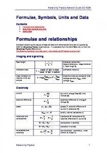
If several branes are on the top of each other, new massless gauge bosons arise from the strings that were previously stretched among branes. The gauge symmetry is enhanced from U (1) × U (1) × · · · to U (n) for a stack of n-branes. There is an equation governing the equality between the the number of bosonic and the number of fermionic worldvolume fields in terms of spacetime and super D-brane worldvolume dimensions similar to the one derived for generic super p-branes. It reads as d − (p + 1) + (p − 1) =
nΘ , 4
(40)
where the first term in the l.h.s. comes from the scalar fields, the second one comes from the extra vector fields and the terms in the r.h.s represent the fermionic degrees of freedom. From it we can table the D-branes in the table bellow named the D-brane scan. The products denote the number of supercharges preserved in each targetspace dimension.
70
4
Branes in M-Theory
In this section we are going to review the extended solutions of supergravity in d=11 dimensions. At present, it is believed that this theory represents the low-energy effective field theory of a more general eleven dimensional quantum theory, named M-Theory which should unify all string theories in a consistent manner. Beside the above assumption, nothing else is known about M-theory except, maybe, a non-covariant formulation of it in terms of D0-branes (particles) known under the name of M(atrix) theory ( see the references). From M-theory point of view, string theories represent d=10 dimensional different phases, related among themselves by dualities. There is a continuously increasing number of evidences that support the dualities which are merely conjenctures. A rigorous proof of them would involve mastering of string theories at both perturbative and nonperturbative level. Although no non-perturbative string theory has been put forward yet, there are a number of tools that allow us to check dualities. They are useful in investigating M-theory, too, and they are based on effective field theories, branes and supersymmetry. In what follows we will review the basics of d=11 supergravity. Then we will review the M2 and M5 branes and finally we will shortly present the algebraic approach to the intersection of M-branes.
4.1
Scales in String Theory
M-theory, which one expects to unify all fundamental interactions, is unknown at present. Anyway, there are reasons to consider that its low-energy effective action should be the d=11 supergravity. One argument that supports this hypothesis is the fact that type IIA and heterotic E8 ×E8 superstrings can be obtained from d=11 supergravity by appropriate compactifications on one spacelike dimension. Let us denote the fundamental string length in ten dimensions by ls and the Planck length in ten and eleven dimensions by l10 and l11 , respectively. Now, if we want to compactify d=11 supergravity to obtain type IIA supergravity, we should consider one of the spacetime directions, say X 11 as being a circle of radius R. In the limit when the fundamental string length α0 = ls2 goes to zero, it follows from Newton’s constant in d=10
71
G2 = gs2 α0 4 that ls > l10 , when gs is the string coupling. On the other hand, the string coupling is given by the vacuum expectation value gs = e which is related to the 3
component of the metric in d=11 dimensions G11,11 = e2σ by e = e 2 σ . Thus, in the perturbative regime, i. e. gs < 1, we conclude that 2
R ∼ gs3 l11 .
(41)
If we want to relate d=11 units to the string units we can use the fact that the Newton constant in d=10 string theory and the one from compactified d=11 theory should coincide G10 ∼
8 gs2 l10
9 G11 l11 ∼ = R R
(42)
,
(43)
from which we see that 1
l11 ∼ gs3 ls
R ∼ gs ls .
The conclusion is that at g ¿ 1, both the eleven dimensional Planck length and the radius of the eleventh dimension are small compared to the string scale and therefore the following relation holds ls > l10 > l11 > R.
(44)
In the interval ls > l10 the gravity from the low-energy effective field theory can be decoupled from the super-Yang-Mills component of the theory as was recently shown in [34, 35, 36] using D-brane technology. In this limit another duality was conjenctured, between the supergravity on AdS spacetime and CFT on its boundary. Let us take a closer look at the compactification of d=11 supergravity. If we take the large R limit in the compactified theory, the Kaluza-Klein modes propagating in this direction become light. But the compactified theory is type IIA supergravity. Therefore, in this theory there should be states of which masses behave like m=
1 1 ∼ . R gs ls
(45)
These are pointlike solitonic objects with vanishing masses in the strong coupling and carrying R-R charge. A simple dimensional analysis gives us the relation between the tension of M2-brane and the tension of the fundamental string. Since the tension of M2-brane is Tm = E/A = 72
−3 l11 where E is the energy and A is the area, and the tension of the fundamental string is
given by Ts = E/L = ls−2 , it follows that the two tensions are related by Tm = gs−1 Ts3/2 .
4.2
Effective Field Theory of M-theory: d=11 supergravity
As we have already noticed, one can interpret the eleven dimensional supergravity as the low energy effective field theory of M-theory. There is a huge literature on this topic going back to 1978 when d=11 sugra was discovered. The eleven dimensions represent a limitation on the dimensionality of spacetime in which supergravity can exist. This limitation is twofold: on physical grounds it reflects the fact that no massless fields with spin greater than 2 and no more than one graviton is permitted. From mathematical point of view, it is related to the Clifford algebras in (1, d−1) dimensions and to the fact that gravitational interactions are incompatible with higher spin gauge fields. d=11 supergravity is also the unique quantum field theory in the sense that only N=1 supersymmetry is allowed and the field content is fixed. The action of d=11 supergravity is given by Z
S=
√ 1 d1 1 −g[k −2 R− FM N P Q F M N P Q +kA∧F ∧F +ψ¯M ΓM N P DN ψP ]+(4f ermi terms), 2 (46)
where k is the Einstein constant, A is the 3-form gauge potential and ψ is the 3/2 gravitino. Indeed, if we count the degrees of freedom we see that we should add to the 44 transverse traceless spatial metric components
(d−2)(d−30(d−4) 3!
d(d−3) 2
=
= 84 transverse spatial
d
components AM N P of the 3-form to obtain 2[ 2 ]−1 × (d − 3) = 128 degrees of freedom of the fermionic spinor-vector gravitino. If we want to obtain type IIA supergravity, we have to perform a Kaluza-Klein compactification. The Kaluza-Klein ansatze reads 4
2
ds2 = e− 3 φ dxµ dxν gµν + e 3 (dy − dxµ Aµ )
(47)
for the d=11 line element and 1 1 A = dxµ dxν dxρ Aµνρ + dxµ ∧ dxν ∧ dyAµν 6 2
73
(48)
for the three form. Here, µ, ν, ρ = 0, 1, . . . , 9 and y is the compactified dimension y ∼ y + 2πR. Before going on and discuss the extended solutions of this theory, let us make a detour to the supersymmetry and see what its role is in the d=11 theory that we study. Let us consider the supersymmetry algebra of d=11 supergravity and focus on the spinor charge anticommutators because they represent the relevant part for our discussion {Qα , Qβ } = (CΓM )αβ PM ,
(49)
where C is the (real, antisymmetric) charge conjugation matrix, Γ’s form a representation of Clifford algebra and PM are the components of momenta. Let us suppose that there is some quantum theory that realizes the algebra (49) and label the vacuum of this theory by |0 >. Since it is supersymmetric invariant we should have Qα |0 >= 0.
(50)
Assume that in this theory there is some (massless) state that preserves some fraction ν of the supersymmetry. Then the following relation should hold < ν|{Qα , Qβ }|ν >≥ 0.
(51)
To determine the number ν we firstly remark that (49) implies that det(ΓM PM ) = (P 2 )16 = 0,
(52)
which means that the momentum of these states is small. If we go to a frame where 1 PM = (−1, 1, 0, . . . , 0) 2
(53)
and if we chose the Majorana representation (in which C = Γ0 ), we can recast (49) in the following form 1 {Qα , Qβ } = (1 − Γ01 )αβ , 2
(54)
where Γ01 = Γ0 Γ1 . (It is easy to verify that Γ201 = 1 which implies that its eigenvalues are ±1. Also, since T rΓ01 = 0, half of the eigenvalues are +1 and half are -1.) Now, for the states with zero eigenvalue, (54) gives us Γ01 ² = ±². 74
(55)
Thus, from all that was said above, we see that ν = 1/2 and that massless states |ν > preserve half of the supersymmetry algebra (49). These states can be associated to the massless superparticles which have the following action in Minkowski vacuum Z
S[X, Θ, e] =
1 ¯ M Θ)2 , dτ (X˙ M − iΘΓ e
(56)
where e(τ ) is an independent worldline scalar density, X M (τ ) are the bosonic fields and Θα (τ ) are their fermionic superparteners. The action (56) is invariant under (rigid) superPoincar´e transformations δX M = i¯²ΓM Θ δΘ = ²
(57)
with the spinor parameter ²(tau). The superparticle does not break all supersymmetries since there is also a kappa-symmetry of the action ¯ M δk Θ δk X M = iΘΓ δk Θ = 6 P k(τ ).
(58)
If we use the light-cone gauge in which Γ = Θ = 0, where Γ± = 21 (Γ0 ± Γ10 ), we see that the gauge fixed theory has sixteen linearly realized symmetries. Thus, the superparticle breaks half of the supersymmetries of the background field theory which has (49) as a symmetry. Return now to the supersymmetry in d=11. Let us express the Lagrangian of the action (46) in terms of vielbeins and write down the indices (for pedagogical reasons). The result is 1 1 1 L = − eR(ω) − eψ¯M ΓM N R DN (ω)ψR − eFM N RS F M N RS 2 2 48 √ i 2 ¯ M N RST LN 3 M1 ···M11 e(ψM Γ ψN + 12ψ¯R ΓST ψ L )FRST L − √ (12) ² FM1 ···M4 FM5 ···M8 AM9 ···M11 − 384 2 4 + (ψ (terms), (59) where e = det(eM A ), M, N, . . . = 0, 1, . . . , 10 are spacetime indices and A, B, . . . = 0, 1, . . . , 10 are tangent-space indices. Also 1 ¯P Q 0 ωM AB = ωM AB + ψ ΓP M ABQ ψ 8 75
(60)
0 where ωM AB is the spin connection in the absence of supersymmetry and DM are the
components of covariant derivative. We also used the notation ΓM1 ···Mn = Γ[M1 · · · ΓMn ] ,
(61)
where the square brackets denote antisymmetrization. The transformations of e, ψ and A under supersymmetry are given by 1 A ²¯Γ ψM 2√ 2 ²¯Γ[M N ψR] = − 8 √ 2 RSLT 0 R SLT ]², = [DM (ω) + (Γ − 8δM Γ )FRSLT 288 M
δeA M = δAM N R δψM
(62)
0 where FM N RS is the supercovariant field strength, given by
3 0 = 24∂[M AN RS] + √ ψ¯[M ΓN R ψS] . FRSLT 2
(63)
The equations of motion derived from (59) are non-linear since they express the interactions. We are interested in finding solutions of these equations that preserve some fraction of the supersymmetry. The bosonic solutions have ψM vanishing. From (62) this implies that the supersymmetric variation of E and A vanish, too. Therefore, the only condition for having a supersymmetric solution is √ 2 RSLT R SLT 0 (Γ − 8δM Γ )FRSLT ]² = 0. δψM = [DM (ω) + 288 M
(64)
Spinor parameters ²0 satisfying this equation are called Killing spinors. Now if we choose a gauge in which F = 0 we have δψM = DM (ω)²0 = 0.
(65)
As we can see from (64) or (65) the Killing spinor condition imposes severe restrictions on the gravitational field. Indeed, applying DM (ω) twice one obtains from (65) DM DN ²0 = 0.
(66)
It is important to notice that under the constraint (65), the equations of motion of supergravity have the following supersymmetric solution ds2 = dudv + k(ξ, u)du2 + dξ · dξ,
76
(67)
where ξ are Cartezian coordinates for E 9 and k is an arbitrary function of u and harmonic on E 9 . The solution (67) is called a ’M-wave’ and it describes an asymptotically flat region at k → 0 as |ξ| → ∞. If this metric is used to compute DM , (65) reduces to Γv ² = 0, where v = t + x1 which is equivalent to Γ01 ² = ². The field ² is assumed to be constant st infinity and its value is taken to be the zero-eigenvalue of {Q, Q}. We can conclude from the above analysis that we have fluctuations of the classical solutions described by Goldstone fields whose effective action is the superparticle action in the light-cone gauge. We can use the fluctuations of M-waves to find the M-branes.
4.3
Branes of M-Theory
From the d=11 supergravity action (46) we derive the equations of motion using the usual variational principle. For the antisymmetric tensor field they are given by 1 d ∗ F + F ∧ F = 0, 2
(68)
from which we can compute the following charge Z
U=
1 (∗F + A ∧ F ), 2 ∂Ms
(69)
where ∂Ms is the boundary at infinity of an arbitrary infinite spacelike 8-dimensional subspace of d=11 spacetime. Similarly, from the Bianchi identity dF = 0,
(70)
we can deduce another charge that is conserved under it, namely Z
V =
˜5 ∂M
F,
(71)
where the surface integral is taken over the boundary at infinity of a spacelike 5dimensional subspace. These charges can be related to an central charge extension of the supersymmetry algebra {Q, Q} = C(ΓM PM + ΓM N UM N + ΓM N P QR VM N P QR ,
(72)
where C is the charge conjugation matrix, MM N and VM N P QR are 2-form and 5-form charges related to U and V , respectively. The l. h. s. of (72) has 528-components since
77
the spinors of d=11 supergravity have 32-components. On the r. h. s. we also have 528 components as follows: 11 for PM , 55 for UM N and 462 for VM N P QR . This sets the match between the number of components in the two sides of (72). The supersymmetry algebra (72) represents a modified version of (49). The physical reason for this modification is the presence of some extended physical objects in supergravity theory. These are a 2-brane (called M2-brane) and a 5-brane (called M5-brane) respectively. Consider firstly an M 2-brane. It arises as a solution of the bosonic part of the action (46) under the ’electric’ ansatz. By choosing appropriate coordinates, we can write this solution in the following form 1
1
ds2 = [R2 (−dt2 + dσ 2 + dρ2 ) + 4k 3 R−2 dR2 ] + k 3 dΩ27 1
1
+ k 3 [(1 − R3 )− 3 − 1][4R−2 dr2 + dΩ27 ] Aµνρ = R3 ²µνρ ,
(73)
where the worldvolume coordinates are xµ = (t, σ, ρ) and dΩ27 is the line element on the unit 7-sphere, corresponding to the boundary ∂M8 and k is an specific integration constant. This form of the solution has several advantages. Firstly, it displays explicitly the inside horizon. At R = 0 with R < 0 being the interior, the light-cones does not ”flip over”. Secondly, we can see from (73) that at R → 1 (the asymptotic exterior) the solution is flat, while at R = 0 (near thee horizon) the last product in the metric vanishes and what is left is the standard form of the metric on (AdS)4 × S 7 . From this we can see that the memebrane interpolates between flat space vacuum at R → 1 and (AdS)4 × SS 7 at the horizon.. Inside the horizon one eventually encounters a timelike singularity as R → −∞. The nature of this singularity suggests that the solution should be coupled to a δ-function and gives the interpretation of the membrane as an electrically charged object. Indeed, the membrane represents the unique matter that consistently couple to d=11 supergravity. Thus, the electric source that couples to supergravity is described by the fundamental membrane action. Its bosonic part is given by Z
S2 = −T2
Σ3
Z
q
d2+1 σ −det(∂µ X M ∂ν X N gM N (X))+Q2
78
σ3
1 ∂µ X M ∂ν X N ∂ρ X R ²µνρ AM N R (X). 3! (74)
If the tension and the electric charge are equal, Q2 = T2 , it turns out that the action is k-symmetric. Varying the action above with respect to A3 , we obtain the following current Z
J M N R = Q2
Σ3
δ 3 (Y − X(σ))dX M ∧ dX N ∧ dX R ,
(75)
that enters the r. h. s. of the equation of motion (68). Thus we can compute the charge as a volume integral of the source Z
U=
M8
∗J(3) = Q2 .
(76)
The action (74) is invariant under the truncation of the first two terms in the r. h. s. of the algebra (72) and the central charge is obtained by an integration over the 2-cycle occupied by the membrane in spacetime Z
Z
MN
= Q2
dX M ∧ dX N .
(77)
Now if we are going to see if a membrane preserves the supersymmetry or not, we take a Majorana representation of the Dirac matrices ( C = Γ0 ) and fix the membrane in, say, 12 plane. We thus take only Z 12 different from zero. The truncation of (72) in this setting is given by {Q, Q} = P 0 + Γ012 Z12 ,
(78)
and the l.h.ss. of the equation above is clearly positive. P 0 should be nonzero since the sign of Z 12 can be flipped if the membrane is replaced by an antimembrane. For P 0 = 0 we have the vacuum,, while for P 0 > 0 we have that P 0 ≥ |Z12 | ∼ T2 ≥ |Q2 |.
(79)
If the membrane is stable it saturates the bound, i. e. T2 = |Q2 |. In this case (78) becomes {Q, Q} = P 0 [1 ± Γ012 ].
(80)
For spinors that satisfy Γ012 ² = ±², since (Γ012 )2 = 1 and T rΓ012 = 0, results that the dimension of the zero-eigenvalue eigenspaces of {Q, Q} is sixteen. The conclusion is that the membrane saturating the bound (79) preserves half of the supersymmetry of the vacuum.
79
Let us turn to the 5-brane solution of the d=11 supergravity. This solution represents a magnetic 5-brane and in the same coordinates as the ones used in the case of the membrane, it reads as ds
2
2
µ
2 3
ν
= R dx dx ηµν + k [
Fm1 ...m4 = 3k²m1 ...m4 p
4R−2
2
8
(1 − R6 ) 3
dR +
yp r5
dΩ2 4 2
(1 − R6 ) 3 (81)
where µ, ν = 0, . . . , 5 are the worldvolume indices and m1 , , . . . , m4 ,p = 6, . . . , 11 are transverse space indices. The surface at R = 0 represents a nondegenerate horizon. The light-cones maintain their timelike orientation when crossing the horizon as in the membrane case. These is an important symmetry of the 5-brane, namely a discrete izometry R → −R. This allows us to identify the spacetime regions R ≤ 0 and R ≥ 0 which means that the sets −1 < R ≤ 0 and 0 ≤ R < 1 should also be identified. The asymptotic limits R → −1 and R → +1 are indistinguishable and they describe regions of flat geometry. Thus there is no singularity in the 5-brane. However, there is a throat at the horizon with the (AdS)7 × S 4 geometry down the throat instead of (AdS)4 × S 7 in the membrane solution. The 5-brane spacetime (81) is geodesically complete, so the solution is completely non-singular which shows that the charge carried by the 5-brane is a magnetic charge. Indeed, the field strength is purely transverse as one can see from (81), so no electric charge is present. Since in the integral there is just one orientation that gives a contribution (the surface transversal to the d=6 worldvolume), we can write down the charge of the 5-brane Z
V =
∂M5T
npqr dΣm , (4) ²mnpqr F
(82)
where dΣm (4) is the surface integral over the boundary of M5T which is the transverse space. This charge is preserved by topological properties of spacetime, and thus M 5 is a solitonic solution of supergravity. The M5-brane field content consists in five bosons associated to the transversal coordinates (which are also Nambu-Goldstone bosons of the broken translational invariance and worldvolume fields), and eight fermions. In order to fix the mismatch of the bosonic and fermionic degrees of freedom, one should also add a self-dual two-form B (∗dB = dB). One can then write down the low energy effective action which has the following bosonic
80
sector Z
q
˜ + q1 ˜ IJ HIJK ∂ K a] H d σ[ −det(g + iH) 4 (∂a)2 Z 1 + (C6 + H ∧ C(3) ), 2 WV
S =
6
(83)
where C6 is the pull-back of C6 , C3 is the pull-back of C(3) , a is a non-dynamical field, and ˜ IJ = H
6
1
q
(∂a)2
²IJKLM N ∂K aHLM N
˜ KL , ˜ IJ = √ 1 gI gJ H H −detg K K
(84)
where I, J = 0, . . . , 5. We see that the covariant action (83) is clearly non-local due to the presence of a. Let us count the number of supersymmetries preserved by the 5-brane. To this end we are going to use the same procedure as for the membrane. We first go to a Majorana representation and fix the brane in some directions, say 12345,, with Y12345 6= 0. Let us define Y = Y12345 /P 0 . The algebra corresponding to (72) and truncated to the first and last term in r. h. s. is given by {Q, Q} = P 0 [1 − Γ012345 ].
(85)
In Majorana representation Q’s are real, so we can talk about the positiveness of the above commutator. Since this should be positive, using the properties of Γ012345 we see that Y should satisfy |Y | ≤ 1.
(86)
Now, if the bound of the above equation is saturated, we have sixteen zero eigenvalues of {Q, Q} if the parameters of the corresponding susy transformation satisfy Γ012345 ² = ².
(87)
From that we conclude that the M5-brane preserves half of the supersymmetries of the background. Before ending this paragraph, let us make some remarks. Let us introduce for M2- and M5-branes the following ADM energy density
81
Z
E=
∂MT
dd−p−1 ΣM (∂ n hmn − ∂m hbb ),
(88)
where ∂MT is the boundary transverse space and hmn are the components of the metric in the asymptotically flat expansion gM N = ηM N +hM N . Here, m = p, . . . , 10 runs over the transverse diresction. The relation above is valid for any p-brane solution. In this setting the Bogomol’ny bound read for electric and magnetic branes as follows
2 E≥√ U ∆ 2 E≥√ V ∆
,
electric bound
,
magnetic bound,
(89)
where ∆ is some specific number and U and V are the electric and magnetic charges, respectively. Both M2- and M5-branes saturate this bound, i. e. E2 = U , E5 = V,
(90)
which make these objects BPS-states. This is another way to see that the branes of Mtheory preserve half of the supersymmetries of the background.
5
Intersecting Branes
As we saw in the precedent sections, all low-energy effective actions of string theories as well as d=11 supergravity, admit extended solutions. These are characterized by some supersymmetry and by a charge. The solutions that preserve half of the supersymmetry of the background and satisfy a BPS-bound are particularly important in investigating the non-perturbative aspects of superstrings. In particular, the Dp-branes play a central role. We have described diverse quantum field theories corresponding to branes and we have seen that these are supersymmetric field theories that realize half of the supersymmetries of the background. Let us turn our attention to some other field theories that emerge from branes, more exactly from the intersection of branes. We will limit in this section only to the branes of M-theory.
82
For the present purposes, it is useful to write the brane solutions of d=11 supergravity, namely the ones given previously in (73) and (81) in isotropic coordinates. The M2-brane takes the following form 1
ds2 = H 3 [H −1 (−dt2 + dx21 + dx22 ) + (dx23 + · · · dx210 )] c ∂α H , H = H(x3 , . . . x10 ) , ∇2 H = 0 , c = ±1, Ft12m = 2 2 H
(91)
where H is an harmonic function depending on the transverse coordinates. If we take H =1+
a , r = |~x| r6
(92)
we have just one membrane with the worldvolume oriented along the hyperplane {0, 1, 2} q
and located at r =
x23 + · · · x210 = 0. If we generalize (92) to several centres H =1+
k X aI I=1
rI6
, rI = |~x − ~xI |
(93)
we describe k parallel M2-branes located at positions ~xI . The M5-brane solution is given by 2
ds2 = H 3 [H −1 (−dt2 + dx21 + · · · + dx25 ) + (dx26 + · · · + dx210 )] c Fα1 ···αn = ²α ···α ∂α H , H = H(x6 , . . . , x10 ) , c = ±1, 2 1 5 5
(94)
where ²α1...α5 is the flat d=5 alternating symbol. For a single M5-brane one chooses H =1+
a , r = |~x|, r4
(95)
while for k parallel M5-branes we have H =1+
k X aI I=1
rI4
, rI = |~x − ~xI |.
(96)
Let us denots an M2-brane localized in {0, 1, 2} directions and an M5-brane localized in {0, 1, 2, 3, 4, 5} directions by
M2 1 2 − − − − − − − − M5 1 2 3
4
5 − − − − −
83
For the intersection of two M2-branes we can have different configurations according to their displacement in spacetime like, for example
M2 1
2 − − − − − − − −
M5 − − 3
4 − − − − − −
or
M2 1 2 − − − − − − − − M5 − 2 3 − − − − − − −
The difference between the above configurations is that in the first case the intersection contains just one point, the origin of the hyperplanes, while in the second case it contains the real axis. Therefore, we will label the first configuration by (0|M 2M 2) and the second one by (1|M 2M 2), respectively. Examples of other intersections of branes of d=11 supergravity are
M5 1 2 3 4
5 − − − − −
M5 1 2 3 − − 6
7 − − −
and
M2 1 2 − − − − − − − − M5 1 − 3
4
5
84
6 − − − −
labeled, according to our notations, by (3|M 5M 5) and (1|M 2M 5), respectively. The corresponding analytic solutions can be found by ”overlapping” (91) and (94). The (0|M 2M 2) solution is given by 1
ds2 = (H1 H2 ) 3 [−(H1 H2 )−1 dt2 + H1−1 (dx21 + dx22 )
Ft12α
+ H2−1 (dx23 + dx24 ) + (dx25 + · · · + dx210 )] c 1 ∂α H 1 c2 ∂α H2 = , Ft34α = 2 2 H1 2 H22
(97)
where Hi = Hi (x5 , . . . , x10 ),∇2 Hi = 0,ci = ±1,α = 5, . . . , 10 and i = 1, 2. Here, Hi are harmonic in the coordinates {x5 , . . . , ξ10 }. If we take these functions of the following form Hi = 1 +
ai , ri = |~x − ~xi |, ri4
(98)
we have a membrane oriented in {1, 2} plane, at ~x1 and another one in the {3, 4} plane at ~x2 which overlap in a point and are orthogonal to each other. A generalization is given by Hi = 1 +
ki X ai,I I=1
4 ri,I
, ri,I = |~x − ~xi,I |
(99)
which describes k1 parallel membranes with {1, 2} orientation and ~x1,I positions and k2 parallel membranes with {3, 4} orientation and located at ~x2,I . The (1|M 2M 5) solution is given by 2
1
ds2 = H13 H23 [H1−1 H2−1 (−dt2 + dx21 ) + H1−1 (dx22 + · · · dx25 )
F6αβγ
+ H2−1 (dx26 ) + (dx27 + · · · + dx210 )] c1 c2 ∂α H2 = ²αβγδ ∂δ H1 , Ft16α = , Hi = Hi (x7 , . . . , x10 ), 2 2 H22
(100)
where ²αβγδ is the d=4 flat space alternating symbol. The (3|M 5M 5) solution is given by 2
ds2 = (H − 1H − 2) 3 [(H1 H2 )−1 (−dt2 + dx21 + · · · + sx23 ) + H1−1 (dx24 + dx25 )
F67αβ
+ H2−1 (dx26 + dx27 ) + (dx28 + dx29 + dx210 )] c1 c2 = ²αβγ ∂γ H1 , F45αβ = ²αβγ ∂γ H2 , Hi = Hi (x8 , x9 , x10 ). 2 2
(101)
Let us analyze the supersymmetries of these intersections. They are made out of 1/2 susy preserved by each object which an associated constraint of the type Γ² = e,
85
(102)
where Γ is some antisymmetric product of gamma matrices and satisfies Γ2 = 1 and T rΓ = 0. Now let us take two such matrices, Γ and Γ0 associated to two branes that intersect and let us denote the carge/tension rations by ζ and ζ 0 , respectively. The supersymmetry algebra contains an anticommutator of the form {Q, Q} = P 0 [1 + ζΓ + ζ 0 Γ0 ].
(103)
In a real representation, the positivity bound imposes some constraints on ζ and ζ 0 depending of the commutation relation [Γ, Γ0 ]. If {Γ, Γ0 } = 0 the following relation holds 2
(ζΓ + ζ 0 Γ0 )2 = ζ 2 + ζ 0 .
(104)
The bound ζ 2 + ζ 0 2 ≤ 1 is equivalent to T ≥ |Z| + |Z 0 |,
(105)
where Z and Z 0 are the charges of the two branes. If this bound is saturated, (103) can be written as {Q, Q} = 2P 0 [ζΠ + ζ 0 Π0 ],
(106)
where Π = (1/2)(1 − Γ) and Π0 = (1/2)(1 − Γ0 ) commute. A zero eigenvalue eigenspinor of {Q, Q} must be annihilated by both of Π and Π0 . That implies that the following relations should be simultaneously satisfied Γ² = ² ,
Γ0 ² = ².
(107)
Now since T r(ΓΓ0 ) = 0, the two matrices Γ and Γ0 can be simultaneously brought to the form 16
z
}|
z
}|
16
{ z
}|
{ z
}|
{
Γ = diag(1, . . . , 1, −1, . . . , −1) Γ
0
8
8
{ z
8
}|
{ z
8
}|
{
= diag(1, . . . , 1, −1, . . . , −1, 1, . . . , 1, −1, . . . , −1).
(108)
Thus, this structure preserves 1/4 supersymmetry. At present there is no theory that describes the worldvolume field theory of an intersection of branes in a consistent manner. However, we note that a configuration of two
86
intersecting branes should appear in the worldvolume field theory as a soliton preserving half of the worldvolume supersymmetry. In this algebraic approach the spacetime interpretation of a worldvolume p-brane preserving 1/2 supersymmetry is completely encoded in the worldvolume supersymmetry algebra. Remarkably, all 1/4 supersymmetric intersections can be obtained as 1/2 supersymmetric solutions of the worldvolume field equations of various M-branes. Let us take the maximal central charge extension of d=6 worldvolume supertranslations algebra of M5-branes [IJ]
{QIα , QJβ } = ΩIJ Pαβ + Y[αβ] + Z (IJ) , ΩIJ Y [IJ] = 0,
(109)
where α, β = 1, . . . , 4 is an index of SU ∗ (4) ' Spin(5) and I, J = 1, . . . 4 are Sp(2) indices. Here, ΩIJ is an Sp(2) invariant antisymmetric tensor, Y is a worlvolume 1-form and Z is a worldvolume self-dual 3-form. These charges are associated to the 1/2 supersymmetric string and 3-brane, respectively. However, there are more charges than corresponding worldvolume objects, which suggest that in the worldvolume physics, the spacetime identification: 1-p-form ↔ 1-object no longer holds. In this case, the number of charges are given by the respresentations of Sp(2) and the interpretation is that Sp(2) representations provide the information needed to reconstruct the branes within branes, the intersecting branes, etc. To clarify the content of the above statement, let us consider Sp(2) as the double cover of SO(5) transverse to the M5-brane worldvolume. Then the space components of the 1-form Y define a vector in the transverse five dimensional space. The associated worldvolume 1-brane can be considered as the boundary of an M2-brane in M5-brane. But the 5 representation of Sp(2) can be interpreted as a 4-form in the transverse space, and thus the associated 1-brane should be interpreted as the intersection of the M5-brane with another M5-brane. The time components of Y can be viewed as the space components of of a dual 5-form which can be interpreted as an M5-brane inside another M5-brane. In the case when 5 representation of Sp(2) defines a 1-form in the transverse space, the interpretation of the time components of Y is that of a 6-brane and the configuration described is that of a 5-brane inside a 6-brane. The corresponding ’6-brane’ of M-theory is in fact the Kaluza-Klein (KK) monopole, so we have an M5-brane inside KK-monopole. Similarly, taking the 5 representation to define a 4-form, the time components of Y give
87
us an M5-brane inside an ’9-brane’ which is in fact the M-boundary. In a similar manner one can interpret the components of the 3-form Z. The same reasoning can be applied to M2-brane if one starts with the N=8 d=3 worldvolume superalgebra (ij)
{Qiα , Qjβ } = δ ij P(αβ) + Z(αβ) + ²αβ z [ij] , δij Z (ij) = 0,
(110)
where Qi are eight d=3 Majorana spinors and i = 1, . . . , 8. Due to the SO(8) automorphism group of this algebra, the 0-form and 1-form centralcharges transform as chiral SO(8) spinors. We are not going to elaborate further on this topic, but rather refer the reader to ([39]). We note, however, that the worlvolume p-brane solitons which describe intersecting branes carry p-form charges which can be expressed as integrals of local charge densities. For example, in the case of the following intersections
M2 1
2 − − − − − − − −
M2 − − 3
4 − − − − − −
and
M2 1 − − − − 6 − − − − M5 1 2
3
4
5 − − − − −
the charges are given by Z
Z
34
=
Z 3
M2
dx ∧ dx
4
6
, Y =
W4
dx6 ∧ H,
(111)
where W4 is spanned by x2 , x3 , x4 , x5 and H is the worldvolume 3-form field-strength of M5 .
88
References [1] M. Green, J. Schwarz and E. Witten, Superstring Theory, vol. 1 and 2, Cambridge University Press (1986) [2] J. Polchinski, Superstring Theory, vol. 1 and 2, Cambridge University Press (1998) a ust and S. Theisen, Lectures on String Theory, Springer-Verlag (1989) [3] D. L¨ [4] H. Ooguri and Z. Yin, TASI Lectures on Perturbative String Theories, hepth/9612254 [5] E. Kiritsis, Introduction to Superstring Theory, hep-th/9709062 [6] J. Polchinski, TASI Lectures on D-branes, hep-th/9611050 [7] J. Polchinski, S. Chandhuri and C. V. Johnson, Notes on D-branes, hep-th/9602052 [8] C. G´omez and R. Hern´andez, Fields, Strings and Branes, hep-th/9711102 [9] L. Alvarez-Gaum´e and M. A. V´azquez-Mozo, Topics in String Theory and Quantum Gravity, Les Houches Lectures, Session LVII, B. Julia and J. Zinn-Justin, eds. (1992) [10] C. P. Bachas, Lectures on D-branes, hep-th/9806199 [11] A. Sen, An Introduction to Non-perturbative String Theory, hep-th/9802051 [12] C. Vafa, Lectures on Strings and Dualities, hep-th/9702201 [13] M. Cederwall, Worldvolume fields and background coupling of branes, hep-th/9806151 [14] W. Taylor, Lectures on D-branes, Gauge Theory and M(atrices), hep-th/9801182 [15] A. Giveon and D. Kutasov, Brane Dynamics and Gauge Theory, hep-th/9802067 [16] E. T. Akhmedov, Black Hole Thermodynamics from the point of view of Superstring Theory, hep-th/9711153 [17] M. J. Duff, R. R. Khuri and J. X. Lu, String Solitons, hep-th/9412184
89
[18] M. J. Duff, Supermemebranes, hep-th/9611203 [19] K. S. Stelle, Lectures on Supergravity p-branes, hep-th/9701088 [20] B. De Wit and J. Louis, Supersymmetry and Duality in Various Dimensions, hepth/9801132 [21] J. G. Russo, BPS bound states, supermemetranes and T-duality in M-theory, hepth/9703118 [22] S. F¨orste and J. Louis, Duality in String Theory, hep-th/9612192 [23] M. J. Duff, A Layman’s Guide to M-Theory, hep-th/9805177 [24] M. J. Duff, M-Theory ( The Theory formerly known as Strings), hep-th/9608117 [25] P. K. Townsend, Four Lectures on M-Theory, hep-th/9612121 [26] P. K. Townsend, M-Theory from its Superalgebra, hep-th/9712004 [27] J. P. Gauntlett, Intersecting branes, hep-th/9705011 [28] A. Giveon, M. Porrati and E. Rabinovici, Target Space Duality in String Theory, hep-th/9401139 [29] J. H. Schwarz, Lectures on Superstring and M Theory Dualities, hep-th/9607201 [30] J. H. Schwarz, From Superstrings on M Theory, hep-th/9807135 [31] J. H. Schwarz, Beyone Gauge Theories, hep-th/9807195 [32] I. Bandos, P. Pasti, D. Sorokin and M. Tonin, Superbrane Action and Geometrical Approach, hep-th/9705064 [33] I. Bandos, K. Lechner, A. Nurmagambetov, P. Pasti, D. Sorokin and M. Tonin, Covariant Action for the Super-Five-Brane of M-Theory, Phys. Rev. Lett.78(1997)43324334
90
[34] J. Maldacena, The large N-limit of the superconformal field theories and supergravity, hep-th/9711200 [35] S. S. Gubser, I. R. Klebanov and A. M. Polyakov, Gauge theory correlators from non-critical string theory, hep-th/9802109 [36] E. Witten, Anti-de Sitter space and holography, hep-th/9802150 [37] R. Argurio, Branes Physics in M-Theory, PhD thesis, Universit´e Libre de Bruxelles (1998) [38] B. Pioline, Aspects non perturbatifs de la th´eorie des supercordes, PhD thesis, Universit´e Paris VI (1998) [39] E. Bergshoeff, J. Gomis and P. K. Townsend, M-brane intersections from worldvolume superalgebras, hep-th/9711043
91


![[PDF] Spacetime Physics John Archibald Wheeler ... - Google Sites](https://m.moam.info/img/260x300/pdf-spacetime-physics-john-archibald-wheeler-googl_64783764097c474e708c90fe.jpg)