Spatial and temporal distribution of sea turtles related

Revista de Biología Marina y Oceanografía Vol. 52, N°2: 377-387, agosto 2017

ARTICLE

Spatial and temporal distribution of sea turtles related to sea surface temperature and chlorophyll-a in Mexican Central Pacific waters Distribución espacial y temporal de tortugas marinas asociada a la temperatura superficial del mar y clorofila-a en aguas del Pacífico Central Mexicano

Karen M. Zepeda-Borja1, Christian D. Ortega-Ortiz1, Ernesto Torres-Orozco1 and Aramis Olivos-Ortiz2 1

Facultad de Ciencias Marinas, Universidad de Colima, Carretera Manzanillo-Barra de Navidad km 20, Col. El Naranjo, C.P.28860, Manzanillo, Colima, México. [email protected] 2 Centro Universitario de Investigaciones Oceanológicas, Universidad de Colima, Carretera Manzanillo-Barra de Navidad km 20, Col. El Naranjo, C.P.28860, Manzanillo, Colima, México Resumen.- En este estudio se describe la distribución espacio-temporal de tortugas marinas y su relación con parámetros oceanográficos en el Pacífico Central Mexicano (PCM) durante el 2010 (invierno, primavera y otoño). Los resultados muestran variaciones en la distribución de tortugas marinas. En invierno, la distribución de tortugas fue homogénea en áreas costeras y oceánicas; asociadas a la presencia de frentes térmicos debido a la interacción de una corriente de agua cálida del sur y la intrusión de agua fría proveniente del noroeste, así como con los límites de un giro ciclónico. En primavera, la distribución de tortugas se concentró hacia la zona costera y parte central de la zona oceánica, donde prevalecieron los efectos de una surgencia y los límites de un giro ciclónico. El mismo patrón de distribución ocurrió al inicio de otoño, mientras que las condiciones oceanográficas cambiaron para la segunda semana de muestreo, cuando ocurrió la formación de una surgencia costera. Los eventos de apareamiento solo se registraron durante otoño para la tortuga golfina (Lepidochelys olivacea), la especie dominante de la región. Se concluye que en otoño el patrón de distribución de tortugas marinas fue hacia la zona costera del PCM, y se relacionó con actividades de reproducción; mientras que en invierno y primavera este patrón tendió a la región central/oceánica vinculado potencialmente con actividades de forrajeo. Palabras clave: Tortugas marinas, distribución, parámetros oceanográficos, giro ciclónico, surgencia Abstract.- In this study we describe the spatial and temporal distribution of sea turtles and their association with oceanographic parameters in waters of the Mexican Central Pacific (MCP) during 2010 (winter, spring and autumn). Our results showed variations in sea turtle distribution through the sampling year. Sea turtle distribution was homogeneous in coastal and oceanic areas during winter; there was an association with thermal fronts generated by a current of cold water flowing from the northwest and a warm current coming from the south, as well as with the boundaries of a cyclonic gyre. Sea turtles were distributed in the coastal zone and the central part of the oceanic zone in spring, where the effects of a cyclonic gyre and coastal upwelling prevailed. The same distribution trend was recorded at the beginning of autumn, whereas oceanographic characteristics changed during the second sampling week, when upwelling occurred. Mating events were only recorded in autumn for olive ridley sea turtles (Lepidochelys olivacea), the dominant species in the region. It was concluded that sea turtles were distributed in the coastal zone of MCP waters in autumn due to reproductive activities, whereas in winter and spring sea turtles were distributed towards the central/oceanic region, potentially related to foraging activities. Key words: Sea turtles, distribution, oceanographic parameters, cyclonic gyre, upwelling

INTRODUCTION Seven sea turtle species are currently recognized worldwide within the Cheloniidae and Dermochelyidae families (MárquezMillán 1990, 1996). They have complex life cycles that encompass oceanic and coastal ecosystems, and their distribution is affected by biological and ecological factors (Frazier 2001, Bolten 2003). Sea turtle species spend most of their life in oceanic waters (mainly the East Pacific green, leatherback, and olive ridley turtles), with only nesting females

spending significant time on land; however, nesting corresponds to only ~1% of their life cycle. Soon after nesting, females return to the sea where they, along with juveniles, adult males and adult non-nesting females will remain some time in oceanic areas as their principal habitat (Spotila et al. 1997). Sea turtle species are protected by national and international environmental laws, and they are listed at different levels ranging from vulnerable to critically endangered in the IUCN red list;

Vol. 52, N°2, 2017 Revista de Biología Marina y Oceanografía

377

therefore, several ecological parameters need to be investigated to conclude on their conservation status (National Marine Fisheries Service & U.S. Fish and Wildlife Service 1998). The distribution of species is an ecological parameter that contributes to the identification of zones and seasons that could render individuals vulnerable to certain threats, such as fishery bycatch and marine debris ingestion. The latter is considered a potential disturbance agent for sea turtles in the coastal area of the MCP (Diaz-Torres 2014). The olive ridley turtle Lepidochelys olivacea (Eschscholtz, 1829), is the most abundant sea turtle worldwide (MárquezMillán 1990). Distributed along the Pacific, Atlantic and Indian Oceans in tropical and subtropical areas (Pritchard 1969), the olive ridley principally inhabits the oceanic zone during all life stages (Bolten 2003, National Marine Fisheries Service & U.S. Fish and Wildlife Service 1998), where it exploits multiple foraging areas (Plotkin et al. 1994) that are influenced by the presence of coastal upwelling, oceanic fronts and cyclonic gyres (Frazier 2001, Luschi et al. 2003). Olive ridley turtles have been detected in areas of the Eastern Tropical Pacific where oceanographic parameters are variable. For example, Polovina et al. (2004) reported the presence of these turtles in two different kinds of environments in the central part of the Pacific Ocean adjacent to the Hawaiian islands: a) one with low uniform Chlorophyll-a (Chl-a) concentrations and weak current dynamics; and b) a second characterized by high Chl-a concentrations and the presence of strong currents. In contrast, Swimmer et al. (2009) found olive ridleys distributed in areas characterized by relatively high superficial Chl-a concentrations (0.37 mg m-3) and the presence of a cyclonic gyre (Costa Rica Dome). Both studies also reported the aggregation of olive ridley turtles in areas with warm surface temperatures (25-28ºC) (Polovina et al. 2004, Swimmer et al. 2009). Therefore, the spatial and temporal distribution pattern of this species is unclear, and may vary among regions. The coastal region of the Mexican Central Pacific (MCP) has been recognized as a migratory destination for olive ridley turtles to carry out breeding activities during certain seasons (Márquez-Millán 1990, Quijano-Scheggia et al. 2006). Most research about sea turtle ecology is based on data collected on nesting beaches; knowledge has therefore been obtained on only one population component, mature females (Bjorndal 2000). For this reason, any information that encompasses the entire population should be considered valuable. There are no studies that relate oceanographic parameters to sea turtle distribution in the MCP, although several oceanographic processes (at different scales ranging from 10 to 100 km) occur in this region due to the interaction of different

378 Zepeda-Borja et al. Sea turtle distribution in Mexican Central Pacific waters

water masses that converge in the area (Torres-Orozco et al. 2005, Salas-Pérez et al. 2006, López-Sandoval et al. 2009). The present study is considered the first in providing spatial and temporal distribution patterns for sea turtles (undifferentiated adults and juveniles) in MCP waters, using direct observations during at-sea surveys (e.g., Houghton et al. 2006), linking these distribution patterns with oceanographic parameters to demonstrate a potential influence on the ecological activities of sea turtles, such as breeding and feeding.

MATERIALS AND METHODS STUDY AREA The Mexican Central Pacific (MCP) encompasses 87,291 km2 between 16º48.68’-18º07.54’N and 102º5.85’-104º22.17’W. The coastal limits were located to the north at Cabo Corrientes, Jalisco, and to the south at Maruata, Michoacán, with a 180 km extension offshore. The area was divided in two zones parallel to the mainland: coastal (0-40 km) and oceanic (40180 km). The coastal zone was determined by the width of the continental shelf and slope (see Figure 2 and 3 to identify the study area).

FIELD WORK Three research surveys were conducted in 2010 on board the fisheries research vessel BIP XII: 1) winter (15-27 January), 2) spring (25 May-6 June), and 3) autumn (18-29 October). We employed linear transect sampling during daylight hours (7:00-19:00 h) at an average speed of 8-9 knots under favorable sea state conditions (Beaufort scale (B) = 0-3) to guarantee sea turtle detection. Transects were systematically designed as part of a study of sea turtle and marine mammal monitoring; however, vessel routes varied depending on logistic and environmental factors. Sea turtle sightings were recorded by 3 observers located on the highest ship platform (6.7 m above sea level) using Fujinon 7x50 binoculars and facing in different transect directions. The date, hour, sea state (B scale), ship course, number of sea turtles, and reticle number and angle (data supplied by binoculars) were recorded for each sighting. The geographic position of the ship course and observed turtles were recorded using a global positioning system Garmin GPSmap 76cs. If the sea turtle was close to the ship’s transect line, its species and sex (mature males have longer and thicker tails; Márquez-Millán 1990, 1996) were recorded, and a photograph was taken with a Canon digital camera model EOS-50D to corroborate or identify the species from its morphological features, using the guides by Pritchard & Mortimer (2000) and Wyneken (2004).

In addition, mating events (a pair of turtles joined with the male above the female) were recorded during these surveys.

SEA

TURTLE DENSITY CALCULATIONS

To analyze the spatial and temporal trends of sea turtle distribution, and to reduce the bias caused by differences in effort among the zones, the density (Di) of organisms along each transect was calculated as:

possible to record reticle or angle value were omitted from density calculations and statistical analyses. To determine whether there were significant differences in densities among seasons and zones, we used non-parametric Chi-square tests (X 2) with   0.05 significance, using the software ® STATISTICA ver. 7.0.

SEA SURFACE T EMPERATURE

AND

CHLOROPHYLL -a

ANALYSES

where: n is the number of sea turtles recorded along transect i, W is the width and L the length of transect i. The length of the transect (Li) is the distance traveled (in km) from the point where the observation effort started to the point where it stopped, considering the following conditions to discriminate among transects: 1) decrease in speed or lack of navigation, 2) change of course, and 3) change of zone (transition between coastal and oceanic areas). The width of each transect (Wi) was equivalent to the maximum perpendicular distance (with respect to the ship’s course; in km) at which a turtle was observed. Its estimation was obtained by incorporating the reticle number and angle in the equations proposed by Jaramillo-Legorreta et al. (1999). This variable (Wi) could be influenced by the sea state (B scale) observed during each transect, i.e., at a sea state B  1, there was a higher probability of sighting a turtle at a greater distance than at transects with B  3.We therefore obtained a standard Wi for each B scale (0, 1, 2, and 3) for each zone (coastal and oceanic), established by the maximum W value during all transects with a similar B scale value. The corresponding Wi was used to calculate turtle density based on the B scale at which each transect occurred. Only sightings corresponding to the olive ridley sea turtle (L. olivacea) were taken into account for density analyses, as well as sightings of turtles that did not show clear morphological characteristics typical of other species, e.g., large size and longitudinal edges of the shell (Dermochelys coriacea), darker coloration and flatter shell (Chelonia mydas), lighter coloration and shell keels (Eretmochelys imbricata) (Márquez-Millán, 1990). The assumption that these sightings could correspond to olive ridley turtles is supported by the great abundance of this species in adjacent waters of the Mexican Tropical Pacific (Eguchi et al. 2007), as well as along nesting beaches in the area (Quijano-Scheggia et al. 2006). Observations of sea turtles for which it was not 1

Sea Surface Temperature (SST) and Chlorophyll-a (Chl-a) data were obtained from the Aqua Modis (EOS PM) sensor from NASA (NASA’s Ocean Biology Processing Group, OBPG)1, with 4 km spatial resolution. We used images of 8-day composite periods, corresponding to the weeks during which each survey was conducted. Data image processing was carried out using ®R ver. 2.14.1 software (Villalobos & GonzálezRodríguez 2010). To describe the spatial-temporal distribution of sea turtles, we plotted weekly maps of each oceanographic parameter, of sea turtle sightings, and of sampling transects onto a map, using ®MATLAB ver. 7.0 software. We also included geostrophic current data from NOAA: Near Real-Time Altimeter page, calculated from climatic values and sea high anomalies from the Naval Research Laboratory (NRL) (Trinanes 2001). We performed a correlation analysis (Beta,   0.05) between sea turtle densities and SST and Chl-a, by 1) identifying the values of these oceanographic parameters in correspondence to each sea turtle position using the program ® WAM (WIM Automation Module)2; and 2) calculating the average of oceanographic parameters in each line transect to correlate with sea turtle density for the same line transect. Analyses were run using ®STATISTICA ver. 7.0 software.

RESULTS SEA TURTLE DENSITY Sea turtle distribution was homogeneous throughout the study area (coastal: 0.07 turtles km-2; oceanic: 0.05 turtles km-2) (X2= 2.57, = 0.11, n= 97) in winter (Fig. 1; Table 1). We identified more olive ridley sea turtles (21 confirmed sightings) that any other species: East Pacific green turtle (Chelonia mydas, 4 sightings), loggerhead (Caretta caretta, 10 sightings), leatherback (Dermochelys coriacea, 2 sightings), and hawksbill turtles (Eretmochelys imbricata, 2 sightings). The total number of unidentified turtles was 358 (Table 2).

2


379

Sea turtle density in the coastal area (0.53 turtles km-2) was significantly greater than density in the oceanic area (0.07 turtles km-2) (X2= 5.81, = 0.01, n= 119) during spring (Fig. 1; Table 1). Only two species could be identified: olive ridley, which was the most observed (5 sightings) and East Pacific green (1 sighting) (Table 2).

Density in the coastal zone (0.73 turtles km-2) was significantly greater than in the oceanic zone (0.06 turtles km-2) (X2= 5.95, = 0.01, n= 84) during autumn (Fig. 1; Table 1). Two species could be identified: olive ridley turtle, which was the most frequent (12 sightings), and East Pacific green (7 sightings). Mating events were only recorded for olive ridley turtles, and occurred only during autumn (n= 11; Table 2).

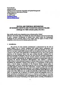
Figure 1. Estimated density of sea turtles by zone in Mexican Central Pacific waters during three seasons in 2010 / Densidad estimada de tortugas marinas por zona en aguas del Pacífico Central Mexicano durante las tres temporadas del 2010

Table 1. Spatial and temporal sea turtle density in coastal and oceanic zones of the Mexican Central Pacific during three seasons in 2010 / Densidad espacial y temporal de tortugas marinas en zonas costeras y oceánicas del Pacífico Central Mexicano durante tres temporadas del 2010


Table 2. Sea turtles sighted in Mexican Central Pacific waters during 2010 / Avistamientos de tortugas marinas en aguas del Pacífico Central Mexicano durante el 2010

On a temporal scale, sea turtle density was highest during autumn (0.32 turtles km-2), followed by spring (0.19 turtles km-2), and winter (0.06 turtles km-2); these differences were not significant, however (X2= 3.56, = 0.17, n= 300) (Table 1).

D ISTR IB U TIO N

OF

SEA

TU RTLES

R ELATED

TO

OCEANOGRAPHIC PARAMETERS

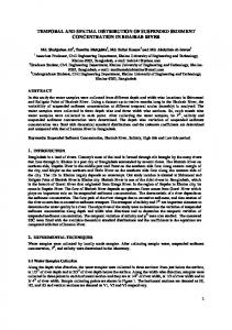
Slightly colder water (25.5-26.4ºC) was detected during winter, flowing from the northwest into the oceanic zone, promoting the formation of thermal fronts (26-27.3°C) where small groups of sea turtles were found (Fig. 2A1). In addition, a warm current (27.2-28.9ºC) from the south was also identified, extending through the coastal zone and the southern part of the oceanic area (Fig. 2A1). Temperature values associated with sea turtles within this warm current were high (27.4-28.9°C) in comparison with that for thermal fronts (Fig. 2A1), whereas Chl-a concentrations were low (0.16-0.25 mg m-3), but similar to values reported for turtles within the cold intrusion water (0.17-0.24 mg m-3) (Fig. 3A1). The correlation between sea turtle density and SST was not significant (Beta= 0.03, = 0.59), nor was it significant for Chl-a (Beta= 0.004, = 0.84). A cyclonic gyre was detected (17.6-18.7°N and 104.6105.9°W) during the second week of winter; it produced a transition zone in the oceanic area, where SST ranged from 26.2 to 28.5°C and Chl-a ranged from 0.2 to 1.4 mg m-3 (Fig. 2A2). Sea turtles were distributed within the transition zone generated by the interaction of the cyclonic gyre and the remnant of cold water intrusion. The SST ranged from 26.5 to 27.6ºC (Fig. 2A2), whereas Chl-a ranged from 0.18 to 0.63 mg m-3 (Fig. 3A2). In contrast, turtles recorded in the coastal zone were located in warmer (27-28.5ºC), and more productive (0.15-2.5 mg m-3) waters (Figs. 2 and 3A2). The correlation between sea turtle density and the oceanographic parameters was not significant (SST: Beta= 0.008, = 0.71; Chl-a: Beta= 0.05, = 0.36).

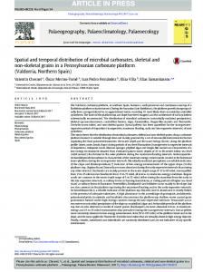
Oceanographic characteristics recorded during two weeks in spring suggested the presence of coastal upwelling off the Jalisco coast, characterized by SST between 24.1 and 25.6ºC (Fig. 2B1-B2) and Chl-a concentrations between 0.57 and 10 mg m-3 (Fig. 3B1-B2). Sea turtles within this area were associated with the boundaries of the upwelling, where high Chl-a gradients were found (0.14-1.8 mg m-3) (Fig. 3B1); however, these values were lower (0.12-0.48 mg m-3) during the second week (Fig. 3B2). In addition, a cyclonic gyre off Colima state (17.8-18.9°N and 104.3-105.7°W), was detected during the two sampling weeks. This gyre resulted in Chl-a concentrations between 0.15 and 0.63 mg m-3 (Figs. 3B1-B2) and SST ranging from 25.9 to 28°C (Figs. 2B1B2). Although the distribution pattern of sea turtles was associated with the boundaries of this gyre (Figs. 2 and 3B1B2), the correlation of sea turtle density with SST and Chl-a during the first (SST: Beta= 0.03, = 0.37; Chl-a: Beta= 0.08, = 0.10) or second week (SST: Beta= 0.03, = 0.47; Chl-a: Beta= 0.03, = 0.45) was not significant. Warmer SST was recorded throughout the entire study area during the first sampling week of autumn (27.3-30ºC). Sea turtles density was highest near the coast, and sea turtles aggregated in two large groups: one near the northern part of Jalisco state (19.5-20ºN) with a relative density of 1.44 turtles km-2, and the other near the southern part of Colima and northern Michoacán (18.2-19ºN), with a relative density of 0.46 turtles km-2. The SST associated with sea turtle positions ranged from 27.4 to 30°C (Fig. 2C1), whereas the Chl-a observed over sea turtle aggregations reflected more productive waters (0.41-10 mg m-3), compared to turtles in the oceanic zone (0.15-0.3 mg m-3) (Fig. 3C1). However, the correlation analysis between sea turtle density and SST and Chl-a was not significant (SST: Beta= 0.02, = 0.55; Chl-a: Beta= 0.0004, = 0.92). We observed coastal upwelling in the second week (SST: 24.1-25.5ºC; Chl-a: 0.75-10 mg m-3), extending from Cabo


381

Corrientes, Jalisco, to the southern part of the study area. This upwelling was also confirmed by the dynamics of the geostrophic currents (Figs. 2 and 3C2). The sea turtles were located over the warm part of the oceanic zone, with an associated SST of 27.4-28.3°C (Fig. 2-C2) and low Chl-a concentration (0.180.37 mg m-3), except for a small turtle aggregation (17.4-17.6ºN and 103.8-104.6ºW), located in a Chl-a front area (0.32-1.17

Figure 2. Distribution of olive ridley turtles (Lepidochelys olivacea, triang les) and unide ntified sea turtles (circles) in relation with Sea Surface Temperature in the Mexican Central Pacific during 2010. A1) Winter: 15-21 January; A2) Winter: 22-27 January. B1) Spring: 25-31 May; B2) Spring: 1-6 June. C1) Autumn: 1823 Octobe r; C2) Autumn: 24-29 October. Black arrows represent geostrophic currents. Solid white line shows the sampling transects. Solid black line represents the division be tw een quadrants. CC= Cabo Corrientes, Jalisco. M= Maruata, Michoacán, Mexico / Distribución de tortugas g olfinas (Lepi dochel ys oli vacea, tr iángulos) y tortug as marinas no identificadas (círculos) en r elaci ón a la temperatura superfi cial del mar del Pací fi co Central Mexicano durante el 2010. A1) Invierno: 15-21 enero; A2) Invierno: 22-27 enero. B1) Primavera: 25-31 mayo; B2) Primavera: 1-6 junio. C1) Otoño: 18-23 octubre; C2) Otoño: 24-29 octubre. Flechas negras representan corrientes geostróficas. Líneas sólidas blancas muestran los tr ansectos de muestreo. Lí neas negr as sólidas representan la división entre cuadrantes. CC= Cabo Corrientes, Jali sco. M= Maruata, Michoacán, México


mg m-3) (Fig. 3-C2). Sea turtles in the Colima coastal area were located in slightly cooler (26.8-28ºC) (Fig. 2-C2) but more productive waters (0.72-2.3 mg m-3) (Fig. 3-C2). The correlation between sea turtle density and both variables was not significant (SST: Beta= 0.10, = 0.24; Chl-a: Beta= 0.05, = 0.38).

Figure 3. Distribution of olive ridley turtles (Lepidochelys olivacea, triangles) and unidentified sea turtles (circles) in relation with Chlorophyll-a concentration in Mexican Central Pacific waters during 2010. A1) Winter: 15-21 January; A2) Winter: 22-27 January. B1) Spring: 25-31 May; B2) Spring: 1-6 June. C1) Autumn: 18-23 October; C2) Autumn: 24-29 October. Black arrows represent geostrophic currents. Solid white line shows the sampling transects. Solid black line represents the division between quadrants. CC= Cabo Corrientes, Jalisco. M= Maruata, Michoacán, Mexico / Distribución de tortugas golfinas (Lepidochelys olivacea, triángulos) y tortugas marinas no identificadas (círculos) en relación a la concentración de Clorofila-a del Pacífico Central Mexicano durante el 2010. A1) Invierno: 15-21 enero; A2) Invierno: 22-27 enero. B1) Primavera: 25-31 mayo; B2) Primavera: 1-6 junio. C1) Otoño: 18-23 octubre; C2) Otoño: 24-29 octubre. Flechas negras representan corrientes geostróficas. Líneas sólidas blancas muestran los transectos de muestreo. Líneas negras sólidas representan la división entre cuadrantes. CC= Cabo Corrientes, Jalisco. M= Maruata, Michoacán, México


383

DISCUSSION This study presents calculations of sea turtle density in waters of the MCP, as well as oceanographic features of the region that could potentially explain the observed spatial-temporal distribution pattern. Most of the sea turtles observed during this study (~93%) were labeled as unidentified species, because we were no able to detect morphological characteristics particular to each species, e.g., large size and longitudinal shell edges for D. coriacea, darker coloration and flatter shell for C. mydas, lighter coloration and shell keels for E. imbricata (Márquez-Millán 1990). It is however possible that most of them corresponded to the olive ridley sea turtle (L. olivacea), which was the most sighted species in the MCP (38 confirmed identifications) compared with the other four identified species (26 identifications, Table 2). In addition, this species is the most abundant in waters of the Mexican Tropical Pacific and Central America (X= 1.38 million, CV= 19.7%, CI: 1.15-1.62 million) (Eguchi et al. 2007), and the nest and hatchlings reports released by sea turtle camps on the Jalisco, Colima and Michoacán coasts have also demonstrated the dominance of this species (Quijano-Scheggia et al. 2006, Trejo-Robles et al. 2006, Comisión Nacional de Áreas Naturales Protegidas & Secretaria de Medio Ambiente y Recursos Naturales 2009). It is important to keep in mind that most sightings recorded during this study in 2010 probably corresponded to the olive ridley sea turtle, but this is only an assumption and for this reason we will refer to them below as ‘sea turtles’. The distribution trends of sea turtles in MCP waters showed clear spatial variations, perhaps related to particular biological and ecological aspects, such as feeding (in winter-spring) and breeding (in autumn) (Plotkin et al. 1994, National Marine Fisheries Service & U.S. Fish and Wildlife Service 1998, Frazier 2001). Oceanographic parameters showed colder SST (25.526.4ºC) in the oceanic zone during winter, due to an intrusion of water from the northwest associated with California Current waters, which arrived as a sub-superficial current that detached itself from the northern region during this season (Kessler 2006, Salas-Pérez et al. 2006). A warm current flowing from the south (27.2-28.9ºC) was also detected, associated with the Pacific Tropical Surface water (Calva-Chávez 2011), the main component of the Mexican Coastal Current (Kessler 2006). These two conditions could have influenced the potential aggregation of sea turtles in the oceanic zone, mainly in the thermal fronts generated by the boundaries of a cyclonic gyre in the central area of the oceanic zone, and by the cold water current from the northwest (Figs. 2A1-A2). This distribution pattern is consistent with information of olive ridley turtles exploring multiple foraging areas, such as oceanic fronts and


convergence areas in pelagic waters (Plotkin et al. 1994, Plotkin 2003). Oceanic fronts are highly productive systems due to the interaction of several water masses with different densities. They promote the formation of convergence and vertical divergence zones that favor the accumulation of organic/inorganic material, enriching biological productivity at different trophic levels (Font et al. 1987, Lalli & Parsons 1997, Miller 2011). This process could have occurred in the oceanic zone during the second week, where more productive waters were located (0.2-1.4 mg m-3), and where turtle aggregations were observed (Fig. 3A2). Pelayo-Martínez (2013) analyzed the in situ response of nutrients, Chlorophyll-a, and zooplankton biomass versus the oceanographic variability in the oceanic/central region of MCP waters during winter, revealing the presence of Euphasiacea, Decapoda and Amphipoda crustacean groups, as well as gelatinous species of the Doliolida group (pyrosomes and salps) (volume: 14-22 ml 1000-3). Foraging activity may have been occurring in the region, as these organisms are important components of the olive ridley diet (Montenegro-Silva et al. 1986, National Marine Fisheries Service & U.S. Fish and Wildlife Service 1998, Polovina et al. 2004). Sea turtle distribution was observed in the coastal zone and the central part of the oceanic area in spring, where a cyclonic gyre again prevailed (Figs. 2 and 3B1-B2), confirming its semipermanence in the region as previously had been reported (Salas-Pérez et al. 2006). The tendency of sea turtles to aggregate in cyclonic gyre areas (Luschi et al. 2003, Swimmer et al. 2009) has been explained by the oceanographic characteristics of cyclonic gyres (shallow thermocline, wide gradients of Chl-a and nutrients), which stimulate enrichment of the trophic chain and the presence of potential prey (Lalli & Parsons 1997). Coastal upwelling was also detected off the Jalisco coast (Figs. 2B1-B2). It resulted in high Chl-a concentration (0.57-10 mg m-3) distributed over the area due to the presence of the cyclonic gyre, and favoring the formation of frontal zones (Figs. 3B1-B2). Previous studies have indicated that coastal upwelling off the Jalisco coast is a cyclic phenomenon that is due mainly to the wind influence (TorresOrozco et al. 2005, López-Sandoval et al. 2009); a period of upwelling intensification during spring has also been noted. According to the wind pattern from the CoastWatch software of NOAA3, it was noted that winds blew parallel to the continent mainly in the west-northwest direction during the spring sampling period, favoring the formation of upwelling due to Ekman transport (Torres-Orozco et al. 2005, Stewart 2008, LópezSandoval et al. 2009). 3

Sea turtles occurred in frontal zones where SST varied between 25.9 and 28ºC (Figs. 2B1-B2), in slightly productive waters (0.12-1.8 mg m-3) (Figs. 3B1-B2), where the principal organisms in the olive ridley turtle diet have also been reported (Pelayo-Martínez 2013). Therefore, we infer that the presence of sea turtles near these oceanographic structures was related to foraging activities, as has been reported by other authors for the Tropical Pacific Ocean (Frazier 2001, Luschi et al. 2003, Polovina et al. 2004, Swimmer et al. 2009). This behavior may be influenced by the narrow continental shelf and by the 4,000 m deep canyon that lies near the coast in the study area (De la Lanza 1991), which leads sea turtles (such as olive ridley turtles) to forage in the mid-water column, and not in benthic areas, as has been proposed based on satellite tracking (McMahon et al. 2007). Sea turtles were distributed throughout the coastal zone in autumn. This could be influenced by breeding activities such as mating and nesting. Olive ridley turtles reproduce from July to January (Márquez-Millán 1990) with a peak in August and September (Aguilar-Olguín et al. 2006, Trejo-Robles et al. 2006). This coincides with the sightings of mating turtles that were recorded only during the autumn survey (Table 2). Most mating events occur before nesting peaks (Márquez-Millán 1990, Godley et al. 2002). As we were not able to conduct a survey before August-September, when we would have expected a higher count of mating events, we cannot provide an exhaustive discussion. Nesting cycles of olive ridley turtles occur every 14 days during solitary events, and every 28 days during synchronized nesting events, termed ‘arribadas’; ridley turtles can therefore nest approximately three times per season (Plotkin 2003, Abreu-Grobois & Plotkin 2008). Thus, the highest density recorded during autumn (0.32 turtles km-2) (Table 1) can be associated with the arrival of olive ridley turtles to mate and nest in the area, which is supported by the previously mentioned numerous beaching arrivals of olive ridley sea turtles to conservation camps. The presence of upwelling off Cabo Corrientes, Jalisco, was also detected in autumn, favoring the enrichment of biological productivity in the coastal zone and part of the oceanic zone (0.75-10 mg m-3) (Figs. 3C1-C2). This could have favored the increase of potential prey for sea turtles, allowing them to feed during their stay near the coast (Lalli & Parsons 1997, Stewart 2008). López-Sandoval et al. (2009) pointed out that Cabo Corrientes is characterized by coastal upwellings all year long, which tend to occur during the relaxation phase that occurs from July to December. The wind 4

recorded during autumn had a north-northwest direction, also blowing parallel to the coast (NOAA)4. This favored the development of coastal upwelling due to Ekman transport (Stewart 2008), also confirmed by the geostrophic current dynamics (Figs. 2 and 3C2). Integrating the information, we can conclude that sea turtle aggregations, for the most part of olive ridley turtles, were recorded in the MCP region during winter-spring, when we would not have expected records of sea turtles due to their migratory behavior. Sea turtle aggregations were found in oceanic areas where potential conditions appropriate for feeding could occur. Autumn aggregations occurred in the coastal zone and were associated chiefly with breeding activities. Given this result, a potential inference could be established: that these sea turtles could not travel to distant locations, and their distribution pattern could have been influenced over a small spatial scale in the MCP, where oceanographic conditions favored their main ecological activities, such as feeding and breeding (Kernohan et al. 2001). Nevertheless, it should be taken into account that 2010 was an atypical year, because during the first months of the year a warmer temperature anomaly prevailed (‘El Niño’), and during last months of the year the anomaly temperature was colder (NOAA)5, and changes in turtle migration patterns in response to ‘El Niño’ were reported (Plotkin 2010). Therefore, we recommend that a similar study be conducted during a typical year to elucidate the distribution pattern of sea turtles as a function of oceanographic parameters. This ecological aspect could contribute substantial information to the knowledge of the ecology of these species, and contribute useful tools for adequate species management, because at present, all sea turtle species are considered in the IUCN (2013) red list.

ACKNOWLEDGMENTS This bachelor research was made possible by the economic support from the Comisión Federal de Electricidad. We thank Emigdio Marín Enríquez for sharing his knowledge of satellite image edition; the Facultad de Ciencias Marinas and Centro Universitario de Investigaciones Oceanológicas (U. de C.) for logistical support; the Secretaría de Medio Ambiente y Recursos Naturales through the Dirección General de Vida Silvestre México for providing the permits SGPA/DGVS/00072/10 to conduct the field research; the BIP XII crew; as well as some students of the Grupo Universitario de Investigación de Mamíferos Marinos (GUIMM) of the U. de C., Technical 5


385

Assistants and Diane Gendron from Centro Interdisciplinario de Ciencias Marinas (CICIMAR) for their assistance in the field; and four anonymous reviewers for providing useful comments to improve the quality of the manuscript.

Font J, J Tintore & PE La Violette. 1987. Localización de frentes oceánicos por teledetección infrarroja. El caso del Mar de Alborán. In: Melia J (ed). II Reunión Nacional del Grupo de Trabajo en Teledetección, pp. 327-336. Unidad de Investigación en Teledetección, Departamento de Termología, Facultad de Física, Universidad de Valencia, Valencia.

LITERATURE CITED

Frazier JG. 2001. Sesión I: Generalidades de la historia de la vida de las tortugas marinas. In: Eckert KL & FA AbreuGrobois (eds). Las tortugas marinas de la región del Gran Caribe. Un diálogo para el manejo regional efectivo, pp. 318. WIDECAST, UICN/CSE Grupo Especialista en Tortugas Marinas (MTSG), WWF y el Programa Ambiental del Caribe del PNUMA,

Abreu-Grobois FA & P Plotkin. 2008. IUNC SSC Marine Turtle Specialist Group Lepidochelys olivacea. The IUCN Red List Assessment of Threatened Species. Version 2014.2. Aguilar-Olguín S, E Carretero-Montes, A HernándezCorona, L Hernández-Jiménez, MC Jiménez-Quiroz, R Márquez-Millán, MC Rivera-Rodríguez, JA TrejoRobles, H Santana-Hernández, FA Silva-Bátiz & JJ Valdez-Flores. 2006 . Actividades de protección, investigación y manejo de tortugas marinas en Colima y Jalisco. En: Jiménez-Quiroz MC & E Espino-Barr (eds). Los recursos pesqueros y acuícolas de Jalisco, Colima y Michoacán, pp. 410-422. INP-SAGARPA, Manzanillo, Colima. Bjorndal K. 2000. Prioridades para la investigación en hábitats de alimentación. En: Eckert K, K Bjorndal, F Abreu-Grobois & M Donnelly (eds). Técnicas de investigación y manejo para la conservación de las tortugas marinas. Grupo Especialista en Tortugas Marinas UICN/CSE Publicación 4: 1-13. Bolten BA. 2003. Variation in sea turtle life history patterns: neritic vs. oceanic developmental stages. In: Lutz LP, AJ Musick & J Wyneken (eds). The biology of sea turtles 2: 243-257. CRC Press, Boca Raton. Calva-Chávez MA. 2011. Aspectos hidrográficos en la región central del Pacífico mexicano durante 2010. Tesis de Licenciatura, Facultad de Ciencias Marinas, Universidad de Colima. Manzanillo, Colima, 57 pp. Comisión Nacional de Áreas Naturales Protegidas & Secretaria de Medio Ambiente y Recursos Naturales. 2009. Ficha de identificación no. 1 Lepidochelys olivacea. Secretaría del Medio Ambiente y Recursos Naturales, México. De la Lanza EG. 1991. Oceanografía de mares mexicanos, 569 pp. AGT, México. Díaz-Torres E. 2014. Basura marina: agente de disturbio biológico en el Pacífico Central Mexicano. Tesis de Maestría, Facultad de Ciencias Marinas, Universidad de Colima, Manzanillo, Colima, 137 pp. Eguchi T, T Gerrodette, RL Pitman, JA Seminoff & PH Dutton. 2007. At-sea density and abundance estimates of the olive ridley turtle Lepidochelys olivacea in the eastern tropical Pacific. Endangered Species Research 3(2): 191203.


Godley BJ, S Richardson, AC Broderick, MS Coyne, F Glen & GC Hays. 2002. Long-term satellite telemetry of the movements and habitat utilization by green turtles in the Mediterranean. Ecography 25: 352-362. Houghton JDR, TK Doyle, MW Wilson, J Davenport & GC Hays. 2006. Jellyfish aggregations and leatherback turtle foraging patterns in a temperate coastal environment. Ecology 87(8): 1967-1972. IUCN. 2013. IUCN Red list of threatened species. Version 2013.1. International Union for Conservation of Nature Jaramillo-Legorreta AM, L Rojas-Bracho & T Gerrodette. 1999. A new abundance estimate for vaquita: First step for recovery. Marine Mammal Science 15(4): 957-973. Kernohan BJ, RA Gitzen & JJ Millspaugh. 2001. Analysis of animal space use and movements. In: Millspaugh JJ & JM Marzluff (eds). Radio tracking and animal populations, pp. 125-166. Academic Press, San Diego. Kessler WS. 2006. The circulation of the eastern Tropical Pacific: A review. Progress in Oceanography 69(2-4): 181217. Lalli MC & RT Parsons. 1997. Biological oceanography an introduction, 320 pp. Elsevier Butterworth-Heinemann, Oxford. López-Sandoval DC, JR Lara-Lara, MF Lavín, S ÁlvarezBorrego & G Gaxiola-Castro. 2009. Productividad primaria en el Pacífico oriental tropical adyacente a Cabo Corrientes, México. Ciencias Marinas 35(2): 169-182. Luschi P, GC Hays & F Papi. 2003. A review of long-distance movements by marine turtles, and the possible role of ocean currents. Oikos 103(2): 293-302. Márquez-Millán R. 1990. FAO Species Catalogue. Vol. 11. Sea turtles of the world. An annotated and illustrated catalogue of sea turtle species known to date. FAO Fisheries Synopsis 125(11): 1-81. Márquez-Millán R. 1996. Las tortugas marinas y nuestro tiempo, 197 pp. Fondo de Cultura Económica, México.

McMahon CR, CJ Bradshaw & GC Hays. 2007. Satellite tracking reveals unusual diving characteristics for a marine reptile, the olive ridley turtle Lepidochelys olivacea. Marine Ecology Progress Series 329: 239-252.

Bjorndal, FA Abreu-Grobois & M Donnelly (eds). Técnicas de investigación y manejo para la conservación de las tortugas marinas. Grupo Especialista en Tortugas Marinas UICN/ CSE, Publicación 4: 23-41, Washington.

Miller PI. 2011. Case study 16: Detection and visualization of oceanic fronts from satellite data, with applications for fisheries, marine megafauna and marine protected areas. In: Morales J, V Stuart, T Platt & S Sathyendranath (eds). Handbook of satellite remote sensing image interpretation: applications for marine living resources, conservation and management, pp. 229-239. EU PRESPO & IOCCG, Dartmouth.

Quijano-Scheggia SI, A Olivos-Ortiz, JH GaviñoRodríguez, MA Galicia-Pérez, MT Ruiz-Vallejo & R Pérez-López. 2006. Conservación y protección de la tortuga marina en la costa de Manzanillo, Colima, durante cuatro temporadas de desove (2001-2004). En: JiménezQuiroz MC & E Espino-Barr (eds). Los recursos pesqueros y acuícolas de Jalisco, Colima y Michoacán, pp. 390-397. INP-SAGARPA, México.

Montenegro-Silva BC, NG Bernal-González & A MartínezGuerrero. 1986. Estudio del contenido estomacal de la tortuga marina Lepidochelys olivacea, en la costa de Oaxaca, México. Anales del Instituto de Ciencias del Mar y Limnología, UNAM 13(2): 121-132.

Salas-Pérez J, D Gomis, A Olivos-Ortiz & G García-Uribe. 2006. Seasonal hydrodynamical features on the continental shelf of Colima (west coast of México). Scientia Marina 70(4): 719-726.

National Marine Fisheries Service & U.S. Fish and Wildlife Service. 1998. Recovery plan for U.S. pacific populations of the olive ridley turtle (Lepidochelys olivacea), 52 pp. Silver Spring, Maryland. Pelayo-Martínez GC. 2013. Respuesta de los nutrientes, clorofila y biomasa del zooplancton a la variabilidad hidrológica en el Pacífico Central Mexicano. Tesis de Maestría, Facultad de Ciencias Marinas, Universidad de Colima, Manzanillo, 69 pp. Plotkin P. 2003. Adult migrations and habitat use. In: Lutz LP, AJ Musick & J Wyneken (eds). The biology of sea turtles 2: 225-242. CRC Press, New York. Plotkin P. 2010. Nomadic behaviour of the highly migratory olive ridley sea turtle Lepidochelys olivacea in the eastern tropical Pacific Ocean. Endangered Species Research 13: 33-40. Plotkin PT, RA Byles & DW Owens. 1994. Migratory and reproductive behavior of Lepidochelys olivacea in the eastern Pacific Ocean. In: Schroeder BA & BE Witherington (eds). Proceedings of the Thirteenth Annual Symposium on Sea Turtle Biology and Conservation. NOAA Technical Memorandum NMFS-SEFSC-341: 1-138. Polovina JJ, GH Balazs, EA Howell, DH Parker, MP Seki & PH Dutton. 2004. Forage and migration habitat of loggerhead (Caretta caretta) and olive ridley (Lepidochelys olivacea) sea turtles in the central North Pacific Ocean. Fisheries Oceanography 13(1): 36-51. Pritchard PCH. 1969. Studies of the systematics and reproductive cycles of the genus Lepidochelys. Doctoral Thesis, University of Florida, Florida, 226 pp. Pritchard PCH & JA Mortimer. 2000. Taxonomía, morfología externa e identificación de las especies. En: Eckert KL, KA

Spotila RJ, PM O’Connor & VF Paladino. 1997. Thermal biology. In: Lutz LP & AJ Musick (eds). The biology of sea turtles 1: 297-314. CRC Press, New York. Stewart RH. 2008. Introduction to physical oceanography. Department of Oceanography, Texas A & M University, College Station. Swimmer Y, L Mcnaughton, D Foley, L Moxey & A Nielsen. 2009. Movements of olive ridley sea turtles Lepidochelys olivacea and associated oceanographic features as determined by improved light-based geolocation. Endangered Species Research 10: 245-254. Torres-Orozco E, A Trasviña, A Muhlia-Melo & S OrtegaGarcía. 2005. Dinámica de mesoescala y capturas de atún aleta amarilla en el Pacífico mexicano. Ciencias Marinas 31(4): 671-683. Trejo-Robles JA, RE Carretero-Montes, FA Silva-Bátiz & FJ López-Chávez. 2006. Programa de conservación e investigación de tortugas marinas en el Santuario Playón de Mismaloya, Jalisco. En: Jiménez-Quiroz MC & E EspinoBarr (eds). Los recursos pesqueros y acuícolas de Jalisco, Colima y Michoacán, pp. 398-409. INP-SAGARPA, México. Trinanes JA. 2001. Near real-time altimeter: altimeter page, geostrophic currents and GTS. NOAA/Atlantic Oceanographic and Meteorological Laboratory, Washington, Villalobos H & E González-Rodríguez. 2010. Satin: functions for reading and displaying satellite data for oceanographic applications with R. R package version 0.2. The R User Conference 2009, July 8-10, Agrocampus-Ouest, Rennes. Wyneken J. 2004. La anatomía de las tortugas marinas (versión en español). NOAA Technical Memorandum NMFSSEFSC-470: 1-72.

Received 5 August 2016 and accepted 5 July 2017 Editor: Claudia Bustos D.


387