Spin-Anisotropy Commensurable Chains: Quantum Group

arXiv:hep-th/9302001v1 1 Feb 1993

Spin-Anisotropy Commensurable Chains: Quantum Group Symmetries and N = 2 SUSY Alexander B´erkovich, C´esar G´omez and Germ´an Sierra Instituto de Matem´aticas y F´ısica Fundamental, CSIC Serrano 123. Madrid, SPAIN January 1993

Abstract In this paper we consider a class of the 2D integrable models. These models are higher spin XXZ chains with an extra condition of the commensurability between spin and anisotropy. The mathematics underlying this commensurability is provided by the quantum groups with deformation parameter being an Nth root of unity. Our discussion covers a range of topics including new integrable deformations, thermodynamics, conformal behaviour, S-matrices and magnetization. The emerging picture strongly depends on the N-parity. For the N even case at the commensurable point, S-matrices factorize into N = 2 supersymmetric Sine-Gordon matrix and an RSOS piece. The physics of an N odd case is rather different. Here, the supersymmetry does not manifest itself and the bootstrap hypothesis fails. Away from the commensurable point, we find an unusual magnetic behaviour. The magnetization of our chains depends on the sign of the external magnetic field.

Introduction and Discussion Symmetry is the driving concept in particle physics. In Quantum Field Theory the particles are defined as finite dimensional irreps of the space-time and internal symmetry groups. In Statistical Mechanics the notion of symmetry has also played a very important role in the past, as a way of characterizing degrees of freedom and types of interaction. The recently introduced quantum groups are another stride in this direction, which deepens our understanding of symmetry in systems with an infinite number of degrees of freedom. Quantum groups shed new light on the number of difficult problems which are, essentially, non perturbative in nature; determination of the particle spectrum, scattering matrices, correlation functions, to name just a few. ˆ An important family of integrable models is based on the quantum affine algebras Uq (G) [1]. These models are characterized by the quantum deformation parameter q and a finite d and the ˆ The famous six-vertex model corresponds to G ˆ = Sl(2) dimensional irrep of G. d [3], [4] can be constructed fundamental spin 1/2 irrep. [2]. The higher spin versions of Uq (Sl(2)) by fusion procedure [5]. Generally, the spectrum of these models is expected to satisfy the bootstrap axioms [6]: there is a fundamental particle such that all others can be interpreted as bound states. For the isotropic models of spin j (q = 1) the particle spectrum consists of a fundamental spin 1/2 particle which has (for j > 1/2) extra hidden RSOS spin [7], [8]. The corresponding physical S-matrix factorizes into the product of the XXX S-matrix and an RSOS piece. This picture remains essentially unchanged in the semiclassical weak anisotropic 3j , i.e. that of a regime [8], [9]. The central extension for these nearly isotropic models is c = j+1 SU(2)k W ZW model with level k = 2j. Moreover, the excitations above the ground state can be understood in terms of the free bosonic and Z2j -parafermionic [10] degrees of freedom [11]. There is a connection between N = 2 integrable field theories in two dimensions and quantum affine algebras at roots of unity. This became clear in the study of the Sine-Gordon model in ref. [12] and more recently in [13]. The N = 2 structure of the Sine-Gordon models appears at the special value β 2 = 8π3/2 which yields q 4 = 1 ( q = eiπ/p , p = β 2 /(8π − β 2 )) with the SUSY realized in a non local way [14], namely, the one defined by the non local action of the quantum group generators [15]. The solitonic S-matrix of the N = 2 theories factorizes into an N = 0 RSOS S-matrix and the N = 2 S-matrix of the Sine-Gordon model at β 2 = 8π3/2 [16]. 1

Observe that this factorization of the S-matrices is similar to the one obtained for the physical S-matrices of higher spin XXX models using Bethe ansantz techniques. The only difference is that the XXX piece of the S-matrix is replaced in the case of the N = 2 models by the Sine-Gordon XX S-matrix (i.e. the one which corresponds to q 4 = 1). One could wonder at this point whether there exist spin chains whose S-matrices factorize as those of the N = 2 models. We shall give an example of these later. d Commensurability for Uq (Sl(2))-models appears whenever the deformation parameter q is an Nth-root (q N = 1), and the dimension of the irrep used in constructing the model is N ′ (N ′ = N (N/2) if N odd (even)). For N even the commensurable point determines the frontier of the weak anisotropic regime. The first result that we obtain comes from the explicit solution of the Bethe equations for the N even case. From a technical point of view the novelty of the Bethe ansatz analysis is related to the fact that 2j + 1 is not a so called Takahashi number, an assumption that is done in previous studies of higher spin models [9], [17], [26]. The elementary excitations S-matrix has the same structure as that of N = 2 SUSY models, namely, a SineGordon XX S-matrix multiplied by an RSOS matrix associated with graph A2j+2 . This fact iπ suggests that the commensurable spin j-chain with q = e 2j+1 provides a lattice model of N = 2 integrable theories. There is another important reason to study the spin-anisotropy commensurable hamiltonians, namely, the peculiarities of representation theory of quantum groups at root of unity [19]. At these values of q there appear new central elements, that is, new casimirs which form a closed Hopf subalgebra and whose continuous spectrum labels the irreps. Thus, one can change in a continuous way the irrep without changing its dimension. The models so obtained are the non-fusion descendants of the six-vertex model without classical q = 1 analog. The Chiral Potts model constructed from a class of irreps called cyclic, is one example of the latter [20]. In this paper we shall limit our attention to a very special class of the non-classical irreps which we call nilpotent [21], [22], [23]. These irreps have the highest and lowest weights. For the nilpotent deformations of the N even commensurable model we find a similar spectrum and the same central extension as for the commensurable point. The main difference is a replacement of the XX part of the physical S-matrices by the nilpotent R-matrix with N = 4. This nilpotent R-matrix is related to an XX chain placed in the external magnetic field. However, the RSOS piece of the whole S-matrix remains unchanged. The N = 4 nilpotent R-matrix discussed above is, naturally, associated with the quantum algebra Uqˆ(Gl(1, 1)), where qˆ is fixed by the casimir which describes the nilpotent irreps. Since the Gl(1, 1) algebra underlies N = 2 SUSY, we suggest that our nilpotent case is related to the qˆ-deformed N = 2 SUSY. Another issue of interest appears while studying the behaviour of the nilpotent chains under the action of external magnetic field. The external magnetic field acts on all degrees of freedom, while the ”nilpotent” magnetic field acts effectively only on the XX part. The net effect is

2

that the magnetization depends on the sign of the external magnetic field. The magnitude of this effect is proportional to the ratio of the XX degrees of freedom to the total number of degrees of freedom (i.e. it decreases for higher N). We extend our analysis to commensurable spin chains with q N = 1 and N odd. The picture we obtain is drastically different from that of the N even case. The particle spectrum consists of the three types of particles whose energies do not satisfy bootstrap relations. The scattering shifts among these particles are the product of an RSOS piece associated with graph A2jef f +2 with jef f = j/2 (notice the renormalization of the spin) and another RSOS part associated with the ”spin 1” model p = 2, r = 6 [24]. The (p=2,r=6) RSOS model captures most of the aspects of our model: counting of states, central extensions and scattering shifts. However, there is a mismatch in energies, which reveals some failure of the bootstrap. For the N odd case we find no trace of the N = 2 SUSY structure, but this is not surprising, since SUSY always requires an even number of degrees of freedom to be present. An attractive possibility will be to interpret the N odd case in terms of a Z3 -parafermionic extension of N = 2 SUSY [16]. Let us summarize the main results we obtained: i) Integrable deformations of the spin chains away from the commensurable point. ii) Extension of the Bethe ansantz analysis to the cases where 2s + 1 is not a Takahashi number. iii) Computation of the S-matrices for the N even and odd cases, and connection with N = 2 SUSY in the N even case. iv) New method of counting degrees of freedom in the vicinity of the ground state. v) Unusual Magnetic properties of the nilpotent models due to a non trivial interplay between an ”internal” magnetic field associated with the nilpotent casimirs and the external magnetic field. The organization of the paper is as follows. In section 1 we present the basic tools for solving the descendent models including a brief description of the algebraic Bethe ansantz. Section 2 contains some basics on the representation theory of quantum groups at roots of unity and a detailed description of the symmetries, R-matrices and hamiltonians based on the nilpotent irreps. In section 3 we discuss the string hypothesis and solve the Bethe equations for the values of the nilpotent parameter, which yield the hermitian hamiltonians. In section 4 we study the N even case, computing the central extensions and the S-matrices with N = 2 SUSY structure. In section 5 we extend this analysis to the N odd case. Finally, in section 6 we study the magnetic properties which depend on the direction of the external magnetic field. The paper ends with concluding remarks and two appendices where technical details are given.

3

1. Six-vertex Model Descendants 1.1

Descendent Models

d Our starting point will be the quantum affine algebra Uq (Sl(2)) ≡ Uq (A1 ) [1]. The finite dimensional irreps of this algebra at level zero can be easily obtained from the finite dimensional irreps of the non affine quantum algebra Uq (Sl(2)) whose generators E, F and K satisfy the well known relation: (1)

E K = q2K E ;

F K = q −2 K F ;

[E, F ] =

K − K −1 q − q −1

(1.1)

Denoting by πj± an irrep of Uq (Sl(2)) of spin j of positive or negative spin parity we have: πj± (E)er = [r] er−1 πj± (F )er = ± [2j − r] er+1

(1.2)

πj± (K)er = ±q 2j−2r er ± where r = 0, 1, . . . , 2j. This representation can be promoted to a finite dimensional irrep πj,u d as follows: of Uq (Sl(2)) ± πj,u (E0 ) = eu πj± (F )

± πj,u (E1 ) = eu πj± (E)

± ± πj,u (F0 ) = e−u πj± (E) πj,u (F1 ) = e−u πj± (F ) ± πj,u (K0 ) = πj± (K −1 )

(1.3)

± πj,u (K1 ) = πj± (K)

where u is called the spectral parameter. Given two irreps πj1 ,u1 and πj2 ,u2 the intertwiner matrix Rj1 ,j2 (u1 − u2 ) is defined by: Rj1 ,j2 (u1 − u2 ) πj1 ,u1 ⊗ πj2 ,u2 ∆(a) = πj1 ,u1 ⊗ πj2 ,u2 ∆′ (a)Rj1 ,j2 (u1 − u2 )

(1.4)

The intertwiners (1.4) satisfy the Yang-Baxter equation with spectral parameter:

j1 ,j2 j1 ,j3 j2 ,j3 j2 ,j3 j1 ,j3 j1 ,j2 R12 (u1 −u2 ) R13 (u1 −u3 ) R23 (u2 −u3 ) = R23 (u2 −u3 ) R13 (u1 −u3 ) R23 (u1 −u2 ) (1.5)

4

In fact, the intertwiner R-matrices, obtained through solving (1.4), are the trigonometric solutions to the Yang-Baxter equation (1.5) and give rise to the integrable vertex models if one identifies the Boltzmann weights with the intertwiners Rj1 ,j2 1 . The simplest vertex model where the previous construction applies is nothing but the six-vertex model [2] which corresponds to the choice j1 = j2 = 1/2. Taking into account the fact that the spin 1/2 is a fundamental irrep of Uq (Sl(2)), one calls the (j1 , j2 )-models descendants of the six-vertex model. Given the intertwiner Rj1 ,j2 (u) one proceeds, in the spirit of [25], to construct the monodromy and transfer matrices: i)Monodromy matrix: T j1 ,j2 (u) = Rj1 ,j2 (u)a,L Rj1 ,j2 (u)a,L−1 · · · Rj1 ,j2 (u)a,1

(1.6)

where L is the number of sites of the chain and T j1 ,j2 is a (2j1 + 1) × (2j1 + 1) matrix which belongs to End(⊗L V j2 ). ii) Transfer matrix: tj1 ,j2 (u) = T r(T j1,j2 (u)) (1.7) From the Yang-Baxter equation (1.5), which is a consequence of the quasitriangularity of d Uq (Sl(2)), one gets the commutativity of the transfer matrices: h

i

tj1 ,j (u1 ), tj2 ,j (u2 ) = 0

(1.8)

which implies, in particular, that the transfer matrices of the (j, j)-model can be simultaneously diagonalized together with the one of the (1/2, j)-model. The main advantage of this result is that the algebraic Bethe ansantz can be easily extended to the (j, j)-models.

1.2

Algebraic Bethe Ansantz for Higher Spin

Let us, first, consider the case of a quantum deformation parameter q not equal to the root of unity. We shall briefly summarize the algebraic Bethe ansantz for a vertex model of spin j. The basic tools that one needs are : i) Reference state: |Ωj >= ej0 ⊗ · · · ⊗ ej0

ej0 =

1

       

1 0 .. . 0

       

∈ C 2j+1

(1.9)

Writing u as hu and q as eh and taking the limit h → 0 one gets the rational solutions depending on u.

5

ii) Spin-wave creation operator: h

i

(1.10)

h

i

(1.11)

Cj (u) |Ωj >= 0

(1.12)

Bj (u) = T 1/2,j (u)

1,0

Recall that T 1/2,j (u) is a 2×2 matrix. The action of the Bj (u) operator on the reference state (1.9) reduces the total spin of this state by one and creates a spin wave whose quasimomenta depends on the spectral parameter u. iii) Spin-wave annihilation operator: Cj (u) = T 1/2,j (u)

0,1

Since the spin j irrep is a highest weight vector irrep it follows:

Thanks to (1.8) the candidates for the eigenvectors of the transfer matrix t1/2,j are of the Q form m i=1 Bj (ui ): (Aj (u) + Dj (u))

m Y

Bj (ui)|Ωj >= Λj (u, ui)

m Y

Bj (ui )|Ωj >

(1.13)

i=1

i=1

where Aj (u) = (T 1/2,j (u))0,0 , Dj (u) = (T 1/2,j (u))1,1

(1.14)

The conditions on the spin-wave rapidities ui imposed by (1.13) can be easily obtained using the commutation relations between the creation operators Bj (u) and Aj (u) and Dj (u). These commutation relations are encoded in the famous RTT=TTR equation which follows from the definition of the monodromy operators and the Yang-Baxter relation (1.5): j1 j j1 j2 R12 T1j1 j T2j2 j = T2j2 j T1j1 j R12

(1.15)

where T1 = T ⊗ 1, T2 = 1 ⊗ T2 . Taking j1 = j3 = 1/2, j2 = j, we get the desired commutation relations. Indeed, equation (1.15) defines a so called Yang-Baxter algebra whose ”structure constants” are determined by the six-vertex R-matrix R1/2,1/2 . Since the irrep πj is a h.w.v. representation, one deduces that Aj (u) and Dj (u) are (2j+1) × (2j+1) diagonal matrices. Defining aj (u) and bj (u) as:

Aj (u)|Ωj >= (aj (u))L|Ωj > , Bj (u)|Ωj >= (bj (u))L |Ωj > the Bethe equations for the rapidities ui read:

6

(1.16)

aj (ul ) bj (ul )

!L

=

M Y

a(uk − ul )b(ul − uk ) k6=l,k=1 a(ul − uk )b(uk − ul )

(1.17)

where a(u) = a1/2 (u) and b(u) = b1/2 (u). Notice that only the l.h.s. of equation (1.17) depends on j, the r.h.s., corresponding to the six-vertex model, is the same for the whole family of descendants. It will be convenient for later use to introduce the following change of variables: u → γ2 (u − i). In terms of these new variables, the Bethe equations become: sinh γ2 (ul + 2j i) sinh γ2 (ul − 2j i)

!L

=

sinh γ2 (ul − uk + 2i) γ k=1,k6=l sinh 2 (ul − uk − 2i) M Y

(1.18)

The hamiltonian of the spin chain is obtained through the logarithm derivative of the transfer matrix: ∂ Hj (γ) = iI logtj,j (u)|u=0 (1.19) ∂u where I is an overall coupling constant. −1 For j = 1/2 one gets the well known XXZ-chain with anisotropy ∆ = q+q2 = cosγ. In the limit, when the parameter γ goes to zero, one recovers from (1.19) the higher spin isotropic models of the first two refs. in [4]. An example of the spin 1 isotropic hamiltonian is: Hj=1 (γ = 0) =

L X

Si · Si+1 − (Si Si+1 )2

(1.20)

i=1

Within the family of anisotropic higher spin integrable models we shall pay particular attention to the cases where the anisotropy γ and the spin j are commensurable in the sense:

q N = 1,

2j + 1 = N,

N odd

q N = 1, 2j + 1 = N/2, N even

(1.21)

where q = eiγ . At these points, the higher spin XXZ models admit continuous integrable d deformations parametrized by the eigenvalues of the central elements of Uq (Sl(2)) at q N = 1. This will be the subject of the next section.

7

2. New integrable Deformations for qN = 1 2.1

Mathematical Preliminaries: Representation Theory of Uq (Sl(2))

The representation theory of quantum groups at roots of unity has been worked out in full generality in refs. [18], [19]. Here, we will only need the results concerning Uq (Sl(2)), which are summarized below. For q N = 1 the Hopf algebra Uq (Sl(2)) contains a central Hopf subalgebra Zq generated by ′ ′ ′ the elements E N , F N and K N , where N ′ = N (N/2) if N is odd (even). The Schur lemma implies that the finite dimensional irreps π are characterized by the eigenvalues of the central elements: π(a) = ξπ (a)1 , a ∈ Zq

(2.1)

The finite dimensional irreps can then be divided, according to the eigenvalues of the central elements, into the following four types: irrep π cyclic semicyclic nilpotent classical

′

′

ξπ (E N ) ξπ (F N ) x 6= 0 y 6= 0 0 y6= 0 0 0 0 0

′

ξπ (K N ) z 6= ±1 z 6= ±1 generic ±1

dimension N′ N′ N′ ≤ N′

hwv / lwv no/no yes/no yes/yes yes/yes

Table 1. The last two columns reflect the highest and the lowest weight properties of the irreps. The classical irreps are often called regular or restricted. We prefer to use the name ”classical”, in a sense, that they originate from the continuous deformation of the finite dimensional irreps of the classical algebra. In what follows, we shall concentrate on the nilpotent representations. 8

The method of section 1 for constructing the integrable vertex models associated to irreps of quantum groups, can, automatically, be applied to the nilpotent ones. These representations, ′ −1 that we shall denote by πλ , are given in a basis {er }N by: 0

πλ (E)er = dr−1(λ)er−1 πλ (F )er = dr−1 (λ)er+1

(2.2)

πλ (K)er = λq −2r er where

−r

−1 q r

−λ d2r (λ) = [r + 1] λq q−q −1

[x] =

(2.3)

q x −q −x q−q −1

′

′

The eigenvalue of the central element K N is λN . The representation (2.3) has been chosen because the raising operator is the transpose of the lowering one, i.e. (πλ (E))t = πλ (F ). The complex parameter λ ∈ C labels the nilpotent irreps. It is convenient to introduce a ”generalized” spin s by the relation 2 : λ = q 2s , 2s = 2s modN

(2.4)

For generic values of λ, the representation (2.3) is irreducible. There are, however, a finite collection of λ′ s for which the representation is reducible and fully reducible into the direct sum of two classical irreps. This happens for the following values of λ: m ′ λ(±) m = ±q , m = 0, 1, · · · , N − 2

for which ± πλ(±) = πm/2 m

M

± π(N ′ −m−2)/2

(2.5) (2.6)

We will call the values (2.5) orbifold points. Note that they are fixed points under the action of the coadjoint group defined in [19]. Next we want to study certain automorphisms acting on the space of the nilpotent irreps. Let us introduce two discrete transformations called spin-parity (P) and charge conjugation or spin-flip (C) as follows:

λP = −λ , λC = q −2 λ−1 2

Throughout this paper we use j and s to designate ”regular” and nilpotent spins, respectively.

9

(2.7)

From (2.3) one derives the relation between the corresponding irreps:

πλP (E) = iπλ (E) ,

πλC (E) = Cπλ (F )C

πλP (F ) = iπλ (F ) ,

πλC (F ) = Cπλ (E)C

(2.8)

πλP (K) = −πλ (K) , πλC (K) = Cπλ (K −1 )C The charge conjugation matrix C is defined by: C (er ) = eN ′ −r−1

(2.9)

The proof of (2.9) is based on the relation dr (λC ) = dN ′ −r−2 (λ). A representation πλ is called hermitian if [26]: πλ (E)† = vλ πλ (F ) , πλ (K)† = πλ (K −1 )

(2.10)

where vλ = ±1 is a spin-parity of the irrep. Equation (2.10) implies that λ is a phase (i.e. s is real) and that the spin parity depends on the spin s as: sin2γs vs ≡ vλ = sign sinγ

!

(2.11)

In general, equation (2.10) implies certain restrictions on the allowed values of λ : vλ d2r (λ) > 0 f or r = 0, 1, . . . , N ′ − 2

(2.12)

vs sinγk sinγ(2s + 1 − k) > 0 f or k = 1, . . . , N ′ − 1

(2.13)

or equivalently

Hence, for a hermitian irrep the sign of d2r (λ) is independent of r. Our convention for taking the square root is: dr (λ) =

    

1/2 1 λq −r −λ−1 q r −1 [r+1] q−q 1/2  1 λq −r −λ−1 q r 1] − [r+1] q−q−1

[r + 1] i[r +



vλ = 1 vλ = −1

(2.14)

d A hermitian representation πλ of Uq (Sl(2)), when lifted to a representation πλ,u of Uq (Sl(2)), satisfies the following relations:

[πλ,u (E0 )]† = vλ πλ,u (E1 ) [πλ,u (F0 )]† = vλ πλ,u (F1 ) [πλ,u (K0 )]† = πλ,u (K1 ) 10

(2.15)

where we have assumed that u is real. These relations are preserved by the comultiplication. The behaviour of the spin-parity under the discrete symmetries (2.7) is:

vλP = −vλ ,

vλC = vλ

(2.16)

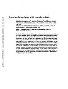
From (2.13) we deduce that the allowed values of the spin s belong to open intervals whose boundaries are the orbifold points (2.6). From now on, for the sake of simplicity, we deal only with cases where q = e2πi/N . The hermiticity intervals for the cases of N even and odd are given in figure 1. We observe that the P-operation interchanges the two spin-parity intervals (i.e. 2s ↔ 2s + N/2), while the C-operation maps each spin-parity interval onto itself leaving invariant the middle point (i.e. 2s → N − 2s − 2). In fact, the middle points of these intervals correspond to classical higher spin irreps whose spin j is commensurable with the denominator of the anisotropy, as in equations (1.21). As can be seen from table 1, these irreps are both classical and nilpotent. The boundaries of the hermiticity regions for q = e2πi/N are the following orbifold points:

N

N even : λ = ±1, ±q 2 −2 N odd : λ = ±q

N−3 2

, ±q

N−1 2

(2.17)

which together with (2.6) impliy that at the orbifold points the hermitian nilpotent irreps break according to the pattern 1 ⊕ N2 for N even and N 2−1 ⊕ N 2+1 for N odd. In appendix A we study, in full generality, the hermiticity regions associated with generic q-primitive root of unity.

2.2

q-Chains Based on Nilpotent Irreps

In this section, we want to find the intertwiner R-matrices associated to the tensor product πλ1 ,u1 ⊗ πλ2 ,u2 . These R-matrices can be found, using a recursive method [27] for solving the intertwiner equations (1.4) in the case of nilpotent irreps. Taking into account the normalization condition 00 R00 =1

(2.18)

we have [22]: 2 −l Rλ1 λ2 (u)rl,r1 ,r1+r = Qr1 +r2 −1 2

j=0

11

(eu λ

1 × −j − e−u q j ) 1 λ2 q

r1 X r2 X







r r [l]![r2 − l2 ]!  1  2  (q − q −1 )r1 −l1 +l2 × [r + l ]![r ]! l l 1 2 2 1 2 l1 =0 l2 =0 ×

r1 +l 2 −1 Y

dj (λ1 )

j=r1

× λl12 λr21 −l1

r1 +l 2 −1 Y

dj (λ1 )

rY 2 −1

dj (λ2 )

j=r2 −l2

j=l1 +l2

r2 −l 2 −1 Y

(eu λ2 q −j − e−u λ1 q j )

r1 +rY 2 −l−1

dj (λ2 )

j=r2 −l2

lY 1 −1

(eu λ1 q −j+r2−l2 − e−u λ2 q j+l2 −r2 )

(2.19)

j=0

j=0

This is another trigonometric solution to the Yang-Baxter equation. Strictly speaking, solution (2.19) comes with a factor q l(r1 +r2 −l)−r1 r2 which can be eliminated under an appropriated rescaling of the basis. Next, we list some useful properties of the R-matrix (2.19): i) Normalization Rλ,λ (u = 0) = P

(2.20) ′

where P is the permutation operator P (v ⊗ w) = w ⊗ v, v, w ∈ C N . ii) Unitarity Rλ1 ,λ2 (u)Rλ1 ,λ2 (−u) = 1

(2.21)

P Rλ1 ,λ2 (u)P = Rλ2 ,λ1 (u)

(2.22)

RλP1 ,λP2 (u) = (1 ⊗ eiπN )Rλ1 ,λ2 (u)(eiπN ⊕ 1)

(2.23)

iii) Parity

iv) Spin-Parity

where N is the number operator: N er = rer

(2.24)

v) Charge-Conjugation RλC1 ,λC2 (u) =

1

(C N ′ −1,N ′ −1 RN ′ −1,N ′ −1 (λ1 , λ2 ; u)

⊗ C)Rλ1 ,λ2 (u)(C ⊗ C)

(2.25)

vi) Hermiticity Rλ† 1 ,λ2 (u) = Rλ1 ,λ2 (−u) 12

(2.26)

This last equation holds true when both irreps λ1 and λ2 are hermitian and have the same spin parity. It reflects the fact that the dagger operation is compatible with the comultiplication b of Uq (Sl(2)), namely: [πλ1 ,u1 ⊗ πλ2 ,u2 (∆(E0 ))]† = vs1 πλ1 ,u1 ⊗ πλ2 ,u2 (∆(E1 )) [πλ1 ,u1 ⊗ πλ2 ,u2 (∆(F0 ))]† = vs1 πλ1 ,u1 ⊗ πλ2 ,u2 (∆(F1 ))

(2.27)

Using the R-matrix (2.19) we can define an integrable vertex model whose integrability condition (1.8) reads: [tλ1 ,λ (u1 ), tλ2 ,λ (u2 )] = 0

(2.28)

In this case, the Bethe equations are a generalization of (1.18) to continuous values of the spin: sinh γ2 (uj + 2si) sinh γ2 (uj − 2si)

!L

=

sinh γ2 (uj − uk + 2i) sinh γ2 (uj − uk − 2i) k=1,k6=j M Y

(2.29)

The spin-chain hamiltonian (1.19) will, of course, depend on the spin s: Hλ ≡ Hs (γ) = iI

∂ log tλ,λ (u)|u=0 ∂u

(2.30)

where I is an overall coupling constant. Before giving the general form of these hamiltonians, it is worth to exhibit their properties which follow from those of the R-matrix: i) Hermiticity: If πλ is hermitian then Hλ† = Hλ

(2.31)

PL H λ PL = H λ

(2.32)

ii) Parity where PL is the operator that reverses the order of the sites along the chain. iii) Spin-Parity HλP = ΩHλ Ω†

(2.33)

Q

where Ω = Lj=1 eiπjNj . iv) Charge-Conjugation HλC = V Hλ V − iL

∂ N ′ −1N ′ −1 R ′ (λ, λ; u)|u=0 ′ ∂u N −1N −1

13

(2.34)

Q

where V = Lj=1 Cj . Since Ω and V are unitary operators, we conclude that the hamiltonians associated to λ, λP and λC describe the same physics. Hence, we shall restrict ourselves to a fundamental region of the P and C operations in the λ space. For any value of q we can choose the half intervals going from the classical point up to the orbifold point within a hermiticity region. In the cases where q = e2πi/N , these intervals are given by:

N even :

j ≤ s < j + 1/2

N odd :

j ≤ s < j + 1/4

(2.35)

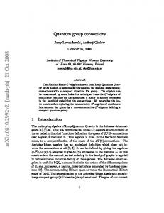
Thus, we have a one parameter family of Hamiltonians Hs (γ = 2π/N) on the interval (2.35), which we can compare with the higher spin XXZ hamiltonians Hj (γ) of section 1. The results of this comparison are graphically presented in figure 2. Along the line I, one continuously modifies the anisotropy γ keeping the spin j fixed, while along the line II, one varies the ”spin”. These two lines meet at a single point A which corresponds exactly to the commensurable higher spin cases of (1.21). A peculiar feature of the nilpotent models (i.e. line II) is the existence of another local conserved quantity obtained by taking the derivative of the transfer matrix with respect to λ1 : ∂ logtλ1 ,λ (u = 0)|λ1 =λ ∂λ1 The counterparts of (2.21 - 2.26) for Qλ are: i) Hermiticity Qλ = 2λ1

(2.36)

Q†λ = Qλ

(2.37)

PL Qλ PL = −Qλ

(2.38)

QλP = −ΩQλ Ω†

(2.39)

QλC = −V Qλ V

(2.40)

ii) Parity

iii) Spin-Parity

iv) Charge-Conjugation

Next, we shall consider a few examples in order to get some insight into the properties of the models we intend to study. 14

Case N=4 The point A of figure 2 has γ = π/2 and j = 1/2 and corresponds simply to the XX model: HXX =

L X

X Y (σiX σi+1 + σiY σi+1 )

(2.41)

i=1

which is equivalent, after a Jordan-Wigner transform, to a free fermion model. Line I of figure 2 corresponds to the XXZ models for different values of the anisotropy γ . The hamiltonians on line II are: Hλ =

L X i (λ + λ−1 ) Z X X Y Y Z (σ σ + σ σ + (σi + σi+1 )) i i+1 λ − λ−1 i=1 i i+1 2

(2.42)

L −i X X (σ X σ Y − σiY σi+1 ) λ − λ−1 i=1 i i+1

(2.43)

and can be recognized as those of the XX models with an external magnetic field given by λ+λ−1 = cosπs. The hermiticity region of (2.42) is 2s ∈ (0, 2) whose boundaries correspond to 2 the critical values of the magnetic field. The operator Q is given by: Qλ =

This is a hopping hamiltonian which is parity odd in contrast with (2.42) which is parity even. Combining these two commuting operators we can construct a hopping hamiltonian with a complex hopping parameter. The hamiltonian (2.42) generalizes the free fermion model in a quantum group symmetric way (the corresponding R-matrix was first introduced [28] from somewhat different point of view). In fact, the nilpotent R-matrix coincides, in this case, with the R-matrix of Gl(1, 1)q (q = λ) in the fundamental representation [29].

Case N=3 The hamiltonians on line I were constructed by Fateev and Zamolodchikov and are associated with the spin 1 XXZ models [3]: HF Z (q) =

L X

Y X + + SkY Sk+1 SkX Sk+1

k=1

X Y − (SkX Sk+1 + SkY Sk+1 )2 −

q 2 + q −2 Z Z Sk Sk+1 2

q 2 + q −2 Z Z 2 (Sk Sk+1) 2

h

X Y Z +(1 − q − q −1 ) (SkX Sk+1 + SkY Sk+1 )SkZ Sk+1 +↔

+

q 2 + q −2 − 2 Z 2 Z [(Sk ) + (Sk+1 )2 ] 2 15

(2.44) i

where S X , S Y and S Z are the classical spin 1 matrices. At the isotropic point γ = 0, (2.44) becomes the hamiltonian (1.20). d with level k = 2j = 2 The later model is gapless and corresponds to a W ZW model SU(2) which has central extension c = 3/2 [8]. The hamiltonians on line II can be written as: H(λ) = −

L X

λq + λ−1 q −1 X X 1 Y Z (Sk Sk+1 + SkY Sk+1 ) − SkZ Sk+1 2 2 sinγ d0 d1 k=1 2 2 1

1 Z X Y )2 −(SkX Sk+1 + SkY Sk+1 )2 + (SkZ Sk+1 2 λq + λ−1 q −1 + + d0 d1 2 −

!

h

X Y Z (SkX Sk+1 + SkY Sk+1 )SkZ Sk+1 +↔

i

(2.45)

 3 Z 2 λq − λ−1 q −1 X X Z Y Z (Sk ) + (Sk+1 )2 − (Sk Sk+1 + SkY Sk+1 )(SkZ + Sk+1 ) 2 2(q − q −1 )

+

 λ2 q −1 − λ−2 q  Z Z S + S k k+1 2(q − q −1 )

which coincides with (2.44) at point A , i.e. λ = q 2 up to an overall factor. From this result we see that the hamiltonian HF Z (q) at q 3 = 1 possesses an additional symmetry given by the operator Qλ with λ = q 2 . In the N = 4 case both hamiltonians Hλ and Qλ were seen to describe the hopping of a free fermion in the presence of a magnetic field. In the N = 3 case one has three degrees of freedom per site. This fact can be accommodated in a model of two fermions A and B subject to the constraint of no double occupancy. Upon the identification e0 → A, e1 → ∅, e2 → B, where ∅ denotes an empty site, we deduce that the hamiltonian (2.45) at λ = q 2 describes the following processes in the terminology of the ref. [30]: 1) Diffusion A + ∅ → ∅ + A, B + ∅ → ∅ + B, A + B → B + A ∅ + A → A + ∅, ∅ + B → B + ∅, B + A → A + B ∅A A∅ HA∅ = H∅A =

B∅ ∅B = = H∅B HB∅

BA AB −HAB = −HBA =−

1 sinγ

(2.46)

where γ = 2π/3. 2) Annihilation A+B

→

∅+∅

B+A

→

∅+∅

∅∅ ∅∅ =− HAB = HBA

16

1 sinγ

(2.47)

3) Creation ∅+∅

→

A+B

∅+∅

→

B+A 1 = − sinγ

AB BA H∅∅ = H∅∅

(2.48)

The hamiltonian has in addition a chemical potential term µ ⊗ 1 + 1 ⊗ µ with :

µA = µB =

1 2sinγ

µ∅ = 0

(2.49)

We obtained a ”chemical interpretation” along the lines of ref. [30] of the hamiltonian Hλ=q2 = HF Z (q 3 = 1). Another interesting hamiltonian emerges when one reaches an orbifold point. As can be seen from (2.45), Hλ has a simple pole at an orbifold point λ0 . Then, it makes sense to define (orb) an orbifold hamiltonian Hλ0 as a residue of Hλ at this point, namely: (orb) Hλ0

= lim

λ→λ0

′ −2 NY

d2r (λ)Hλ

(2.50)

r=0

Choosing λ0 = 1 we get the following ”orbifold” hamiltonian: (orb)

Hλ=1 =

L   1 X − + − − + 0 0 τj+ τj+1 + τj− τj+1 + ρ+ ρ + ρ ρ − σ − σ j j+1 j j+1 j j+1 sinγ j=1

(2.51)

where τ, ρ, σ are different embeddings of Pauli matrices acting in C 3 : τ + = E 12 , ρ+ = E 13 , σ 0 = E 22 + E 33 τ − = E 21 , ρ− = E 31

(2.52)

and E ij is the 3 × 3 matrix with 1 in the i − j position and zeros elsewhere. Eqn. (2.51) has a P P P classical SU(2)×U(1) invariance generated by j σj± , j σ Z , j σ 0 . In ref. [30] this hamiltonian was given a chemical interpretation in terms of diffusion processes only. Another possible interpretation of (2.51) is a Hubbard model with infinite Coulomb repulsion or, equivalently, a t − J model with zero spin-spin coupling. It is known that these models have an infinitely degenerated ground state when L → ∞. This degeneracy is broken in the t − J model by the spin-spin coupling while, in our case, it is broken by the values of λ different from 1. We will further discuss N = 3 case in section 5.

17

Generic N Case Taking into account the complicated structure of the hamiltonian (2.45) for the N = 3 case, it would seem hopeless to find an explicit expression of the hamiltonian for the generic values of N. Fortunately, this is not so and, in fact, we get the following expression: ′

Hλ = −

L NX −1 X

j=1 n=1

n  n i 1 h + − + Σj (λ)Σ− (λ) + Σ (λ)Σ (λ) + µj (λ) + µj+1(λ) j+1 j j+1 sinγn

!

(2.53)

where the matrices Σ± (λ) are given by:

+

Σ (λ)er = Σ− (λ) =



q r − q −r q r−1 λ−1 − q −r+1 λ Σ+ (λ)

†

!1/2

er−1 (2.54)

and µ(λ) e0 = 0 µ(λ) er = −i

r−1 X

λ−1 q j + λq −j er −1 j −j j=0 λ q − λq

(2.55)

In deriving (2.53), we have assumed that λ has a negative parity. The hamiltonian (2.53) exhibits strong formal similarities with the one of the Chiral Potts models [20]: HCP = −

L N −1 h X X



† αn Xj Xj+1

j=1 n=1

n

+α ¯ n Zjn

i

(2.56)

where the coupling constants αn and α ¯ n are given by: 2k−N

ei N φ , α ¯k = αk = sin( πk ) N

¯ i 2k−N φ

k′ e N sin( πk ) N

, cosφ = k ′ cosφ¯

(2.57)

and X and Z satisfy X N = Z N = 1, XZ = e2πi/N ZX. A possible basis for X and Z is: Xer = er−1 modN Zer = e2πir/N er

(2.58)

To bring closer the relationship between (2.53) and (2.56) we will consider the case λ = q −1 and γ = π/N, namely: 18

!

h n  n i 1 2n iπn/N n − + )e Zj )=− Hλ=q−1 (q = e Σ+ + Σ− + (1 − j Σj+1 j Σj+1 πn sin( N ) N j=1 n=1 (2.59) ± ± −1 ± where Σ ≡ Σ (λ = q ) are an N-dimensional version of the Pauli matrices σ (indeed, Σ± = σ ± for N = 2). The origin of the formal similarity between (2.59) and the Chiral Potts hamiltonians is due to the chain of reductions cyclic → semicyclic → nilpotent irreps and the fact that the chiral Potts model is built up from the cyclic irreps. Indeed, if we choose φ = 0 and φ¯ → π/2 in (2.56) we get the same Z terms up to a divergent piece proportional to the number operator. Still, one has to explain why the cyclic operator X reduces to the nilpotent operator Σ+ . Although there are formal similarities between the Chiral Potts model and the one discussed here, we believe that these two models are not equivalent. The main reason is that Chiral Potts preserves a ZN symmetry which is broken in our case. The discussion above suggests that the models we constructed belong to a more general class of integrable theories, whose hamiltonians have the generic structure: iπ/N

L N −1 X X

′

HCN = −

L NX −1 h X



− tn Σ+ j Σj+1

j=1 n=1

n



+ + t¯n Σ− j Σj+1

n

+ hn Zjn

i

(2.60)

This kind of hamiltonians can be obtained through the extension of the Hopf algebra d Uq (Sl(2)) by a central element z with non trivial comultiplications. In this way, the parity is broken and one gets chiral hamiltonians. To end this section, we want to analyze what happens when we reach an orbifold point of the hamiltonian (2.53). If λ approaches ±q m , we see that H (orb) has the block diagonal form I,II II,I HII,I or HI,II , where I and II denotes the two sectors in which the nilpotent irrep breaks at the orbifold point. This means that the only processes taking place are diffusion ones between states which belong to different sectors I + II ↔ II + I.

19

3. Thermodynamics 3.1

Bethe Equations, The String Hypothesis

In this section we will consider in some details the Bethe equations (2.29) with generic spin s in the hermiticity region (2.35). In the thermodynamic limit L → ∞, we will assume the string hypothesis [17]. This means that the solutions to (2.29) are organized into the strings of roots sharing a common real value. These strings are characterized by length n and parity vn as follows: π (n) (3.1) ul = u + i[n + 1 − 2l + (1 − vs vn )] ; l = 1, ..., n 2γ where u represents common the real part and vs is the spin parity introduced in (2.11). Strings of roots can be intuitively interpreted as bound states of the spin waves. From the Bethe equations (2.29) we derive the consistency conditions for the allowed strings (3.1): Y k j=1

(n)



sh γ2 (uj + 2is) (n)



sh γ2 (uj − 2is)

>1;

k = 1, . . . , n − 1

(3.2)

It is not hard to prove that the consistency condition (3.2) for the Takahashi strings (3.1) is equivalent, for asymptotically large rapidities, to the hermiticity condition (2.13) for irreps of dimension n and spin parity vn . In fact, for u → ∞ we get from (3.2): vs

sin(2γs) vn sin(γn) sin γ(n − k) > 0 ; sin γ

k = 1, . . . , n − 1

(3.3)

Using (2.11) we obtain the hermiticity condition (2.13) for irreps of dimension n. Notice that the condition (3.2), for u → ∞, fixes the allowed strings in a form completely independent of the value of the generalized spin s. To feel s we need to consider (3.2) for generic values of the rapidities. We now show that if s is in the hermiticity region (2.35) then the asymptotically allowed strings (3.3) will satisfy (3.2) for arbitrary values of rapidities. To this end we rewrite (3.2) as: k Y

z − cos(y + 2γ(s − j)) >1 j=1 z − cos(y − 2γ(s + j)) 20

(3.4)

where z = chγu; y = γ(n + 1 + p0 1−v2n vs ) and 1 ≤ k ≤ (n − 1). It is straightforward to prove the following identity: k Y

m k−1 X Y z − cos(y + 2γ(s − j)) 2vn vs sin γ(2s − l) sin γ(n − k + l) sin γ(k − l) = 1+ sin γ(l + 1) z − vn vs cos γ(n + 1 − 2k + 2l − 2s) m=0 l=0 j=1 z − cos(y − 2γ(s + j)) (3.5) Taking into account the hermiticity condition (2.13) and the Takahashi condition (3.3) one immediately concludes that l.h.s. of eqn. (3.4) is, indeed, greater than one. Making use of ”Takahashi zone” terminology [17] (also see appendix A) we have, for allowed strings (nj , vj ), the following:

N even :

N

odd :

 

0 − zone nj = j, vnj = +1 1 ≤ j ≤ ν − 1  1 − zone nν = 1, vν = −1 j = ν

            

0 − zone  nj = j, vj = +1  n = 1, v = −1 ν ν 1 − zone  n ν+1 = ν + 1, vν+1 = +1 2 − zone nν+2 = ν, vν+2 = +1

(3.6)

1≤j ≤ν −1 j=ν j =ν+1 j =ν+2

where ν = N2 ( N 2−1 ) for N-even (odd). In the thermodynamic limit, equations (2.29) become: (h)

aj (u) = (−1)rj (ρj + ρj ) +

X

Tjk ∗ ρk

(3.7)

k

(h)

where ρj (ρj ) is density of j-strings (j-holes) and (−1)rj = sign(aj ). The Fourier images of the functions which appear in the equation above are given by:

Tˆjk = g(w; |nj − nk |; vnj vnk ) + g(w; |nj + nk |, vnj vnk ) + min(nj ,nk )−1

X

+2(1 − δ1,min(nj ,nk ) )

g(w; |nj − nk | + 2l; vnj vnk )

l=1

aˆj =

nj −1

X

g(w; 2s + 1 − nj + 2l, vs vnj )

l=0

g(w; n; v) = −

sh2p0 w(( 2pn0 +

1−v )) 4

shp0 w

;

((x)) is Dedekind function

The ”bare” energy of strings of the type j is given by: 21

(3.8)

4π Iaj (u) (3.9) γ where I is an overall coupling constant which is assumed to be positive throughout this paper. Clearly, the equation (3.7) makes sense only if the sign of aj (u) (or Enj (u)) does not change when u varies from zero to infinity. It is a bit surprising that no proof of this fact has been given in the literature. The following is the proof that, indeed, there is no sign crossing for aj (u) as long as nj is an allowed Takahashi string length and s belongs to the hermiticity region (2.35). We represent energy En in the following form: Enj (u) = −

En (z) = − ×{1 +

2Ivn vs sin(2γs) sin(γn) × sin γ[z − vn vs cos γ(2s + n − 1)]

m n−1 X Y

2vn vs sin γ(2s − l) sin γ(n − l) sin γl } m=1 l=1 sin γ(l + 1)[z − vn vs cos γ(2s + n − 2l − 1)]

(3.10)

Once again, making use of formulas (2.13) and (3.3), one can infer that the expression inside of the figure brackets in the equation above is always positive and, therefore, the sign of En is: sign(En ) = −sign[vn vs sin(2γs) sin(γn) sin γ] = −(−1)rj = −(−1)i

(3.11)

with i being a label of the ”Takahashi zone” where nj string lives. Before we move on, let us make the following comment. Irregular spin s, in some sense, plays the role of the ”internal” magnetic field, producing, for instance, the nonvanishing ground state magnetization [22]. However, this interpretation cannot be taken literary because other attributes of magnetic field are absent. For example, none of the string energies change their signs as opposite to the case where system is exposed to the external magnetic field. Renormalized or ”dressed” energy of the string is defined as: (h)

ρ (u) ≡ ηj ; exp [βǫj (u)] = j ρj (u)

β=

1 T

(3.12)

with T being temperature. Equations for the ”dressed” energies can be obtained by minimizing the free energy F X Z +∞ F = −T du|aj (u)|ln(1 + ηj−1 ) L −∞ j

(3.13)

in the presence of the Bethe ansatz constraints (3.5) as was first proposed in ref. [31]. The resulting Dyson like equation is: ln ηj = −4p0 Iβaj +

X

(−1)rk Tjk ∗ ln(1 + ηk−1 )

k

22

(3.14)

Before giving the explicit solution to (3.14) let us briefly comment on its physical meaning. The positive energy strings (and the holes in distribution of negative energy strings) can be interpreted as particle like excitations. The negative energy strings will determine the ground state defined as a state where all negative energy modes are filled. Finally, the zero energy strings reflect the symmetries of the model and will be used to define the internal quantum numbers of all elementary excitations. To solve equation (3.14), it is convenient first to invert the matrix T (see appendix B). Then, this equation can be converted to the following form:

Case N even ln ηj = s1 ∗ [ln(1 + ηj+1 )(1 + ηj−1 ) + δj,ν−2 ln(1 + ην−1 )] ; 1 ≤ j ≤ ν − 2 sin πx Ip0 ] ; r˜ ≡ 0, 1 ln ην−1+˜r = (−1)r˜[s1 ∗ ln(1 + ην−2 ) + πu T ch 2 + (−1)r˜ cos πx Case N odd

(3.15)

ln ηj = s1 ∗ [ln(1 + ηj+1 )(1 + ηj−1 )] + δj,ν−1 [s1 ∗ ln(1 + ηj ) + 4p0 I + (s2 − s1 ) ∗ ln(1 + ην ) − f (u)] ; 1 ≤ j ≤ ν − 1 T −1 ln ην = s2 ∗ ln(1 + ην+1 )(1 + ην+2 )(1 + ην−1 )−1 2Ip0 cos 2πx ln ην+1+˜r = (−1)r˜[s2 ∗ ln(1 + ην ) − ] ; r˜ ≡ 0, 1 T chπu + (−1)r˜ sin 2πx s , l ≡ 1, 2; η0 = 0; x = s − p0 3−v ; fˆ(w) = 2sh( w2 ) chw(2x+1) . where sl (u) = 4l sech πul 2 4 sh2w The equations above can be easily solved in two cases: u → ∞ (or β → 0) and u ≈ 0 [17]. These cases will be important later for the central charge calculations. Results are summarized in table 2 below:

N even 1 + η j = (j + 1)2 ; 1 ≤ j ≤ ν − 2 ην−1 = η −1 ν = ν −1 1 + ηj =

π (j+1) sin2 ν+1 π 2 sin ν+1

N odd 1 + η j = (j + 1)2 ; 1 ≤ j ≤ ν − 1 1 + η ν = η 2ν+1 = (1 + ν −1 )2 η ν+2 = 1 − (1 + ν)−1

; 1 ≤ j ≤ ν − 1 1 + ηj =

ην = ∞

π (j+1) sin2 ν+2 π 2 sin ν+2

1≤j ≤ν−1

; −1

η ν = η ν+1 = ην+2 = ∞ Table 2.

In table 2 above, η = η(∞) and η = η(0). It is relatively simple to convince oneself, using equations (3.15), that all strings are nonnegative except ν − 1 string for N even and ν + 2 for N odd. Making use of this fact, it is now 23

easy to solve equations (3.7) and equation (3.15) in the limit of zero temperature to obtain the following results presented in tables 3 and 4. N even odd

Ground state strings (ρ(h) = 0) ν−1 ν+2

Positive energy strings (ρ = 0) ν ν, ν + 1

Zero energy strings (ρ = ρ(h) = 0) the rest the rest

Table 3. N even odd

Negative Energy

Positive Energy

s) shw(2s−p0 3−v 2 = −ˆ ρ = ν−1 4p0 I sh2w s) ch w shw(2s−p0 3−v bǫν+2 (w) 2 2 = −ˆ ρ = 2 ν+2 4p0 I sh2w

s) shw(2s+2−p0 3−v 2 4p0 I sh2w s) chw(2s+1−p0 3−v bǫν (w) (h) 2 = ρ ˆ = ν 4p0 I chw s) shw(2s+2−p0 3−v (h) bǫν+1 (w) 2 = ρ ˆ ch w2 = 2 ν+1 4p0 I sh2w

bǫν−1 (w)

Table 4.

bǫν (w)

= ρˆν(h) =

The symbol ”hat” in table 4 stands for the Fourier transform. Before finishing this section, we want to point out that the β → 0 limit of the free energy (3.13) provides the justification of the string hypothesis. Indeed, using results collected in table 2 and the formula (3.13), it is easy to obtain: lim β

β→0

X F ′ |aˆj (0)| ln(1 + η −1 =− j ) = − ln N L j

(3.16)

where N ′ = N (N/2) for N odd (even). Equation above implies that the total number of states (N ′ )L is correctly reproduced by the use of the string hypothesis.

24

4. The Commensurable N-even Case: N=2 SUSY From the results of the previous section (tables 3 and 4) we get the relevant information for unraveling the physics of the N even case. To make the resulting picture intuitively more clear, we will begin by considering the commensurable case, point A in figure 2. For generic N even this corresponds to the anisotropic antiferromagnet of spin j = (N 4−2) and anisotropy γ = 2π . N

4.1

Commensurable Case: RSOS-structure

A qualitative picture of the model can be obtained by comparing its string structure with that of the isotropic model with identical spin. In the isotropic case we have the same negative energy strings but a different pattern of the zero energy strings. In fact, all strings with length greater than 2j are allowed and all of them have zero energy. The elementary excitations for the isotropic model are holes in the Dirac sea of 2j-strings. The internal quantum numbers of these elementary excitations are of two types: a ”vertex”-spin with value equal to 1/2 and an ”RSOS”-spin defined by the Coxeter graph of the type A and Coxeter number 2j + 2. These two types of spin determine the dimension of the Hilbert space H(n) with n-holes [8]: dim H(n) = 2n

2j+1 X

K 1i1 . . . K in−1 1 = 2n

2j+1 X i=1

i1 ,...,in−1 =1

πi sin2 ( 2j+2 )

j+1

(2 cos(

πi ))n 2j + 2

(4.1)

with K, the incidence (2j + 1) × (2j + 1) matrix of the graph A2j+2 :

K=



010 101 0 0



... 0 ... 0 . . . 101 . . . 010

(4.2)

The 2n contribution to (4.1) can be effectively obtained by ignoring all the zero energy strings with length smaller than 2j. In fact, the counting of the spin 1/2 degrees of freedom is, 25

essentially, identical to that of the XXX chain. The RSOS-contribution comes from the zero energy strings with length smaller than 2j. For the commensurable case (see table 4), we do not have zero energy strings with length greater than 2j. Instead, we have positive energy negative parity strings of length 1. By drawing analogy with an isotropic case, we may expect the same RSOS structure, but somewhat different ”vertex” spin contribution. From the results collected in tables 3 and 4, we conclude (for N even commensurable case) that the ground state is a Dirac sea of (2j = ν − 1)-strings and that there exist two types of the elementary excitations, degenerate in energy: holes of the Dirac sea and particles associated with the negative parity strings. The particle-hole structure of the commensurable chain is identical to that of XX model. These qualitative arguments indicate that the commensurable chain is equivalent to the free fermions equipped with RSOS-internal degrees of freedom. To prove this claim, we will proceed in step by step fashion: first, computing the dimension of the Hilbert space of n-elementary excitations, then, deriving scattering S- matrix and, finally, calculating the central extension. We start defining the spin Sz of the generic Bethe state |ψ > as a difference in the number of roots with respect to the ground state Sz (|ψ >) = ♯roots(|ψ >) − ♯roots(|Gr. state >)

(4.3)

For N even case we find with a help of the equation (3.7) and the expression for the ground state density (table 4) the following: p0 (h) (˜ nν − n ˜ ν−1 ) (4.4) 2 (h) where n ˜ ν is a number of positive energy strings with negative parity and n ˜ ν−1 is a number of holes in the Dirac ground state. We can interpret (4.4) as a renormalized spin and refer to Sz (|ψ >) =

(h)

n ˜ ν −˜ nν−1 2

as a spin of the state. Recalling that p0 = an integer number, we obtain the restriction (h)

N 2

and taking into account that Sz is always

n ˜ν − n ˜ ν−1 = even integer (p0 odd)

(4.5)

Next, we proceed to compute the dimension of the Hilbert space with n-elementary excitations. The strategy will be to count all degenerate Bethe states containing the total number of particles (ν-strings) and holes equal n. From the hole-particle degeneration, at the commensurable point, we readily get 2n -states. Additional degeneration will correspond to the zero energy strings with length smaller than 2j, i.e. the RSOS part. To count the RSOS degeneration we should, first, invert the equations (3.7) with a help of the inversion formulas presented in appendix B. For N even case we derive (h)

ρ1 + ρ1

(h)

= s1 ∗ ρ2

26

(h)

(h)

ρν−2 +

(h)

= s1 ∗ (ρj+1 + ρj−1 ) ;

ρj + ρj

(h) ρν−2

= s1 ∗

(h) (ρν−3

1

(4.14)

The S-matrices in (4.14) will describe the scattering between the elementary excitations of the model. From the previous counting, we expect that the S-matrix in (4.14) factorizes into the two pieces, each one associated with one of the two different types of spin. 28

The string structure of our model at the commensurable point (i.e. presence of only one string with index greater than 2j and particle-hole degeneracy) can be taken as indication that the spin 1/2 part of the S-matrix must be the one of the XX model. The following is a simple argument to make this claim plausible. In the isotropic case, the singlet and the triplet states differ by the existence of an extra zero energy string of length 2j + 1. This extra string is the reason for the difference between the singlet and triplet S-matrices. In the commensurable case, we do not have this extra string and the ”singlet” (particle-hole) and the ”triplet” (particle(hole)-particle(hole), hole-particle) are practically the same from the point of view of the string content. To get the S-matrices, we will start with the system of eqns (4.6) from which we can obtain: sh(ν − 2)w sh(ν − 2)w |ˆ ǫν−1 | (h) (h) = ρˆν−1 + ρˆν−1 − (ˆ ρν + ρˆν−1 ) + ρˆν−2 + . . . 4p0 I 2chwsh(ν − 1)w sh(ν − 1)w

(4.15)

Note that the equation above has the same structure as the original Bethe ansatz equations (3.7), however, with one important distinction: the roles of ρν and ρν(h) are completely reversed. Let us consider the simplest case: the Bethe state with two holes and one (ν − 2)-string with 2 rapidities u1 , u2 and u1 +u , respectively. The hole-hole S-matrix will contain two contributions: 2 one, coming from the scattering between two (ν − 1)-holes and the other, from the scattering between (ν − 1)-hole and the (ν − 2)-string. These contributions can be directly read from (4.15) Z

dw sh(ν − 2)w sin wu chwsh(ν − 1)w −∞ w Z ∞ sh(ν − 2)w ∂u ln Sν−1,ν−2 (u) = i dw cos wu sh(ν − 1)w −∞ i ln Sν−1,ν−1 (u) = − 2

∞

(4.16)

The hole-hole S-matrix is given by: −i u21 )=e S(u21 ) = Sν−1,ν−1 (u21 )Sν−1,ν−2 ( 2

R∞

dw −∞ w

sin

ν−2 sh 2 w u21 w ν−1 2 sh ch w 2 2 w

×

π ( u221 − i) sh 2(ν−1) π sh 2(ν−1) ( u221 + i)

(4.17)

Using the same technique, we can easily check that the particle-hole and the particle-particle S-matrices are identical to (4.17). This implies that the particle-hole system is, indeed, behaving as XX-chain with respect to the vertex spin. The formula (4.17) gives us the RSOScontribution to the scattering S-matrix. For the case of the two elementary excitations the RSOS contribution is rather simple, in fact, it corresponds to the RSOS-Boltzman weight  

1 2

id



id  (u) 1 2

29

for the A2j+2 -model. Thus, we can represent our S-matrices in the following symbolic form: SXX

O

SRSOS(p=1,r=2j+2)

(4.18)

Notice, that the S-matrix we got, has the same structure as the S-matrix for N = 2 integrable models [16]: S N =2 = SAN2=2

O

=0 SAN2j+2

(4.19)

where SAN2=2 is the Sine-Gordon S-matrix for β 2 = 8π3/2 (which corresponds to q = 1 with β2 q = eiπ/p and p = 8π−β 2 ). The N = 2 SUSY is not explicit in the Sine-Gordon model, but is realized through the quantum group symmetry in the nonlocal way [12], [14].

4.3

Central Extensions

Our analysis of the S-matrices together with the counting of states led us to the conclusion that the commensurable chain is equivalent to the tensor product of an XX spin 1/2-chain and an RSOS model based on the graph A2j+2 . This picture will be consistent if the central charge is given by: 3j N 6 )= ; 2j + 1 = (4.20) c = 1 + (2 − 2j + 2 j+1 2 Two pieces which appear in the sum above are due to the XX and RSOS contributions, respectively. To see that this is, indeed, the case we now proceed to calculate the central extension from the low temperature expansion for the entropy. Following along the standard lines [9], we differentiate the system (3.15) with respect to u and compare the result with the system (4.6). Then, it is trivial to establish asymptotic validity of the following formula: (−1)rj ∂u ǫj 1 ; ρj ≈ 2πvsound 1 + ηj

vsound = p0 I ; u ≫ 1

(4.21)

Plugging (4.21) into the expression for the entropy S XZ S (h) (h) (h) (h) = du[(ρj + ρj ) ln(ρj + ρj ) − ρj ln ρj − ρj ln ρj ] L j

=

XZ

duρj (u)[(1 + ηj ) ln(1 + ηj ) − ηj ln ηj ]

j

30

(4.22)

we obtain S ≈ 2T L

ν X

(−1)rj 1 1 {L( ) − L( )} 1 + ηj 1 + ηj j=1 πvsound

(4.23)

where L stands for the dilogarithmic Roger’s function, defined as ln x ln(1 − x) 1Z x dx{ + } (4.24) 2 0 1−x x Taking η j , η j from table 1 and exploiting ”magic” formulas for the dilogarithmic functions [33]: L(x) = −

 P sin2 π n−2 n   L( )  k=2 sin2 πk  n Pn 1 j=2 L( j 2 )    

2

= (1 − n3 ) π3

= L(x) + L(1 − x) =

π2 6 π2 6

1 − 2L( n+1 )

(4.25)

we, finally, obtain for S and the central extension c the following: 1 2πT L 1 ( − ) vsound 2 ν + 1

(4.26)

3( ν−1 ) 3vsound ∂S = ν−1 2 πT L ∂T +1 2

(4.27)

S≈

c=

Clearly, the formula (4.27) above is in perfect agreement with our prior anticipation (4.20).

4.4

Integrable Deformations

The XX-part of our model, by itself, admits nilpotent extension as we have discussed in section 2. This extension corresponds to an addition of an extra magnetic field coupled only to spin 1/2 degrees of freedom. The product of the nilpotent R-matrix (N = 4) and an RSOS S-matrix λλ RN =4

O

SRSOS(p=1,r=2j+2)

(4.28)

describes our model away from the commensurable point (i.e. for generic spin). To check this claim, we, first, observe that the energies of holes ǫν−1 and particles ǫν presented in table 4 are, essentially, equivalent to those of the nilpotent XX-chain. Second, the RSOS counting formula (4.9) remains valid and so does our central charge result (4.27). Note, however, that the particle-hole degeneracy is now irretrievably lost. We now explain the somewhat surprising result that the central extension does not show any dependence on our nilpotent magnetic field related to the irregular spin s. The point is that this internal magnetic field is selective in nature: it affects only fermionic degrees of freedom, but not RSOS degrees of freedom. Since, the central charge for the free fermions (with or 31

without magnetic field) is equal to 1 and an RSOS part is immune to the internal magnetic field, we conclude that all conformal degrees of freedom are preserved and, therefore, central charge does not change when we move away from the commensurable point. This is contrary to the behaviour of the higher spin XXZ model in the external magnetic field, which freezes out all parafermionic degrees of freedom and reduces the central charge from W ZW -value to just 1. We conclude this section with the following observation. We started by introducing the model based on the nilpotent representation of quantum group. This nilpotency somehow managed to survive the ”hell” of the renormalization (filling in Dirac sea, etc.) and reemerged (like Phoenix) in the modified form in the formula for the physical S-matrices, as expression (4.28) indicates.

32

5. N Odd Case: Beyond Bootstrap For N odd, the commensurable case corresponds to (γ = 2π , j = N 2−1 ). Results collected in N tables 3 and 4 of section 3, clearly indicate that the string structure of the N odd case is a bit more involved than that of the N even case, and the departure from the properties of an isotropic model (γ = 0, j = N 2−1 ) is also more dramatic. First of all, the ground state strings are of length 2jef f with jef f = 2j and not, as it could be naively expected, of length 2j. This circumstance should be interpreted as an indication that for an N odd case our model is in the strong anisotropic regime. The strings with length smaller than 2jef f are of the zero energy which indicates the presence of an RSOS structure based on the A2jef f +2 -graph. The pattern of the positive energy strings is also new. For the N even case, we have only the negative parity strings degenerate in energy with holes of the Dirac sea. For the N odd case, we have two types of positive energy strings: one with length 2j + 3 and another, negative parity string of length 1, designated as (ν + 1) and ν-strings in tables 3 and 4. At the commensurable point, the (ν + 1)-string and the holes of the Dirac sea are degenerate in energy. In this section we will describe some aspects of the system defined by the holes of the Dirac sea and the two positive energy strings in terms of the RSOS model with p = 2 and the restriction parameter r = 6 [24]. The emerging picture is drastically different from the one we have found in the N even case where the model was shown to be equivalent to the tensor product of a vertex XX model and an RSOS model based on the A2j+2 graph. Notice that the (p = 2, r = 6) RSOS model which, for N odd, replaces the XX-part of the N even case, describes the spin 1, SU(2)q -invariant Fateev-Zamolodchikov chain with q 6 = 1 [34].

5.1

Counting of States

The first thing we would like to do is to count the degeneration of the Bethe states following, essentially, the same procedure we used for the N even case. Once again we invert eqns. (3.7) with a help of the identities presented in appendix B to get

(h)

ρj + ρj

(h)

(h)

(h)

= s1 ∗ [ρj+1 + ρj−1 ] + δj,ν−1 [s1 ∗ ρj − 33

− (s2 + s1 ) ∗ ρν(h) + f (u)] ; ρν +

ρν(h)

(h)

ρν+1+˜r + ρν+1+˜r

= s2 ∗

(h) [ρν+1

1≤j ≤ν−1

(5.1)

(h) ρν−1 + r˜

+ ρν+2 ] (−1) cos 2πx = s2 ∗ ρν(h) + ; 2 chπu + (−1)r˜ sin 2πx

r˜ ≡ 0, 1

Here, notations are the same as in section 3. Applying the Fourier transform to the system above and setting w = 0, we derive, after a bit of labor, the following: (h)

n ˜1 + n ˜1

(h)

n ˜j + n ˜j

(h)

n ˜ ν−1 + n ˜ ν−1

1 (h) n ˜ 2 2 1 (h) (h) (˜ n +n ˜ j−1 ) ; = 2 j+1 1 (h) = n ˜ + k˜ 2 ν−2

=

where

1= |˜ nν , n ˜ ν+1 , n ˜ ν+2 > one finds

Sz (|ψ >) = ♯roots(|ψ >) − ♯roots(|Gr. state >) =

N (h) (˜ nν+1 − n ˜ ν+2 ) 2

(5.6)

This implies (for N odd) the restriction (h)

(˜ nν+1 − n ˜ ν+2 ) = even integer

(5.7)

From (5.6) we also observe that the negative parity strings do not contribute to the total spin of the state, which indicates that the ν-string behaves as a spin ”singlet”. Ignoring, for the time being, the zero energy strings, we now proceed to map the Bethe (h) states |˜ nν , n ˜ ν+1 , n ˜ ν+2 > onto the states of the (p = 2, r = 6) RSOS model. This model is defined by the disconnected graph (see fig. 4). We will limit ourselves to the states defined by the first graph I. In terms of this graph we can identify the holes and ν + 1-strings with the 2-point links (j1 , j2 ); |j1 − j2 | = 2 and the ν-string with the closed link (3, 3). We will also impose on the RSOS states periodic boundary conditions. It is easy to check that this identification is compatible with the counting and restriction (5.7) we have described above. (h) In fact, for the given values n ˜ν , n ˜ ν+1 and n ˜ ν+2 , the corresponding number of the RSOS states (h) related to graph I is 2(˜nν+1 +˜nν+2 ) . In this way we capture the ”singlet” nature of the ν-particle. Restriction (5.7) can be easily translated into the RSOS language as a requirement that one should consider only RSOS states which start and finish at the same point on the graph. If we use graph I to describe holes and positive energy strings then we will find, as a basis of the Hilbert space with the total number of n-elementary excitations, the following: (j1 , j2 , . . . , jn+1 ) where

O

(J1 , . . . , JN +1 )

(h)

j1 = jn+1

(h)

J1 = JN +1 = 0

n ˜=n ˜ν + n ˜ ν+1 + n ˜ ν+2 N = 2˜ nν + n ˜ ν+1 + n ˜ ν+2

j ∈ {1, 3, 5} 1 J ∈ {0, , . . . , jef f } 2

(5.8)

(5.9)

and |Ji − Ji+1 | = |ji − ji+1 | =

1 2 

(5.10) (h)



2 f or (˜ nν+1 + n ˜ ν+2 ) couples  0 and ji = 3 f or n ˜ ν couples

States (5.8) for the different partitions of n into the sum of the three positive integers provide a basis of the Hilbert space with n-elementary excitations. 35

The basis (5.8), which is already compatible with our counting, implies that the S-matrix for the elementary excitations is a product of the two RSOS S-matrices. In the next section, we will show that this is, in fact, the case. Before passing to this issue, let us briefly comment on graph II. This graph can be interpreted as describing strings in a discrete target space characterized by the graph A3 [35]. According to this graph, we can suggest the following ”stringy” interpretation. The holes and (ν + 1)-strings can be associated with ”closed” RSOS configurations (2, 2) and (4, 4), and the negative parity string ν with ”open” RSOS configuration (2, 4). If we maintain this ”stringy” interpretation of the graph II, holes and (ν + 1)-strings will appear as bound states of ν-strings.

5.2

S-matrices and Bootstrap

Let us consider the (p = 2, r = 6) RSOS model which is a descendant of the (p = 1, r = 6) model and is obtained by the standard fusion procedure [36]. This model can live in two different regimes: regime (I): The ground state is a Dirac sea of length p = 2-strings and there are no positive energy strings. The central extension is given by: c=

2(p + 2) 3p (1 − )=1; p+2 r(r − p)

(p = 2, r = 6)

regime (II): The ground state is a Dirac sea of length r − 2 = 4-strings. Strings with length 1, 2, 3 = (r − 3) are of the positive energy. Holes are not allowed in the (r − 2) Dirac sea. The central extension is given by: c=2−

6 =1; r

r=6

The elementary excitations in regime (I) are holes of the p = 2 Dirac sea, while in regime (II) they are associated with the positive energy strings. Notice that for (p = 2, r = 6) the central extension is the same in both regimes. To match the dynamics of (ν + 1, ν)-strings and holes of our model we will choose regime (II). The Bethe equations of the (p = 2, r = 6) model can be written as follows [24]: (4)

(h)

aj,2 = ρj +

3 X

(4)

Aj,k ∗ ρk ; 1 ≤ j ≤ 3

k=1 (4)

(4)

with the functions aj,2 and Aj,k best defined by their Fourier transforms: 36

(5.11)

(4)

a ˆj,2 (w) =

1 ˆ(4) A (w) 2ch w2 j,2

(4) Aˆj,k (w) = 2ˆ aj (w)ˆ nk (w) ,

a ˆj (w) =

sh( 4−j w) 2 sh(2w)

j≥k

(5.12)

w kw n ˆ k (w) = cth( )sh( ) 2 2

;

(4) To compute Aˆj,k for j < k we should use the symmetries of the model [24]:

(4) (4) Aˆ1,2 = Aˆ3,2 (4) (4) Aˆ2,3 = Aˆ2,1 (4) (4) Aˆ1,3 = Aˆ3,1

(5.13)

In the regime (II), the positive energies of 1, 2, 3-strings are given by: (4)

ǫj = aj,2

(5.14)

Using (5.12) and (5.13) we conclude that the 1 and 3 strings are degenerate in energy 1 2chw ch( w2 ) = chw

ǫˆ1 = ǫˆ3 = ǫˆ2

(5.15)

This will agree with our counting if we identify the 1 and 3 strings of the (p = 2, r = 6) RSOS model with the holes and ν + 1-strings. However, the energies do not match in a peculiar way. From table 4, we get (up to the overall factor)

ǫˆν+2 = ǫˆν+1 = ǫˆν =

1 chw

ch( w2 ) chw

(5.16)

These are the values for the commensurable point for arbitrary N odd. Comparing (5.15) and (5.16) we, first, observe that for the (p = 2, r = 6) RSOS model the string 2 may be interpreted as a bound states of two 1-strings. The ν + 2-holes and ν + 1-strings have the same energy as 2-string of an RSOS model, however, the negative parity ν-string has twice the energy of the 1, 3 strings. Furthermore, it is straightforward to show that this mismatch of energies persists through the whole hermiticity interval (2.35). Before we give an interpretation of these results, let us see how S-matrices, or better to say, the scattering shifts of the N odd case and (p = 2, r = 6) RSOS model fit together. 37

(4)

The scattering shifts for the interchange of j and k-strings are related to the kernels Aj,k in (5.11). The (p = 2, r = 6) RSOS model is a descendant of the (p = 1, r = 6) RSOS model which completely determines the Bethe strings scattering. The explicit dependence on the value of p = 2 only appears in the energies (5.15) i.e. in the left-hand side of the Bethe eqns (5.11). Using (5.12, 5.13) we find (4) (4) (4) (4) Aˆ1,1 − 1 ≡ Aˆ3,3 − 1 = Aˆ1,3 ≡ Aˆ3,1 =

(4) Aˆ2,3

1 2chw

1 (4) Aˆ2,2 = 1 + chw ch w2 (4) (4) (4) ≡ Aˆ2,1 = Aˆ3,2 ≡ Aˆ1,2 = chw

(a) (b)

(5.17)

(c)

It is important to notice the existence of the extra symmetry reflected in eqns. (a, c) above which is peculiar for the (p = 2, r = 6) model. Using the results above it is trivial to obtain for the S-matrices the following:  

) S1(3),1(3) = tan( π4 + i πu 4 πu π 2  S2,2 = tan ( 4 + i 4 )

(5.18) (h)

Rewriting the Bethe ansatz eqns. (3.7) in such a way that roles of ρν+2 and ρν+2 are reversed, we get ǫˆν 4p0 I

+ + −

ǫˆν+2 4p0 I

ch( w2 ) sh(ν − 1)w (h) (1 − )(ˆ ρν+2 + ρˆν+1 ) + chw shνw sh(ν − 1)w sh(ν − 1)w 1 − − )ˆ ρν + ( chw shνw chwshνw w sh(ν − 1)w w sh(ν − 2)w 2ch( ) ρˆν−1 + 2ch( ) ρˆν−2 + . . . 2 shνw 2 shνw sh(ν − 1)w (h) 1 (h) ρˆν+2 + ρˆν+2 + ( − )(ˆ ρν+2 + ρˆν+1 ) + 2chw 2chwshνw ch( w2 ) sh(ν − 1)w sh(ν − 1)w (1 − )ˆ ρν + ρˆν−1 + . . . chw shνw shνw

= ρˆν + ρˆν(h) +

= +

(5.19)

Reading off the scattering shifts from the r.h.s. of (5.19), we have −i

Shole,hole (u21 ) = e

R∞

−2i

dw −∞ w

R∞

sh(ν−1)w

sin(u21 w) chwshνw

dw −∞ w

×

π u21 ( 2 − i) sh 2ν π πu21 × tan( + i ) π u21 sh 2ν ( 2 + i) 4 4

(5.20) sh(ν−1)w

sin(u21 w) chwshνw

Sν,ν (u21 ) = e π u21 π u21 π u21 sh 2ν ( 2 − i) sh 2ν ( 2 − 32 i) sh 2ν ( 2 − 25 i) πu21 π × ) × tan2 ( + i π u21 π u21 π u21 3 5 sh 2ν ( 2 + i) sh 2ν ( 2 + 2 i) sh 2ν ( 2 + 2 i) 4 4 38

Here, the first expression describes an evolution of the state consisting of two (ν + 2)-holes 2 , respectively. The second one and one (ν − 1)-string with the rapidities u1 , u2 and u1 +u 2 corresponds to the state which has two ν-particles with rapidities (u1 , u2) and one (ν − 2)2 string with the rapidity u1 +u . Let us summarize the salient features of the equations above. 2 They, clearly, indicate that our S-matrix is a product of two distinctly different S-matrices. The first one is related to the RSOS defined by graph A2jef f +2 . The second one is due to (p = 2, r = 6) RSOS model. Note that the second RSOS comes without the usual ”vacuumpolarization” contribution. Also note that ν-string behaves as a bound state of two holes. This is not consistent with our previous result (5.16), thus signaling the breakdown of the bootstrap procedure. Once we have shown the matching of the scattering shifts between the N odd model and N the product of the two RSOS models: (p = 1, r = 2jef f + 2) (p = 2, r = 6) we can return to the question of the energies mismatch we have left open. The reader should be aware that the Bethe study of the scattering shifts we are performing here, is not sufficient to uniquely determine the dynamics of the holes, ν + 1 and ν strings. In fact, the scattering shifts will be the same for (p = 1, r = 6) and for (p = 2, r = 6) RSOS models. Our strategy is to get pieces of the puzzle. First, we observe that the RSOS model with the restriction parameter r = 6 correctly captures the scattering shifts. Second, use of (p = 2, r = 6) RSOS-descendant model leads to the correct counting of the Bethe states, gives the right central extension, however, fails to reproduce energies of the three types of strings which define the spectrum of the N odd case. Two comments are now in order. First of all, a mismatch between bootstrap properties of energies and of scattering shifts is typical of the nonfusion models and, therefore, we can imagine that the model we are seeking is some nonfusion descendant of the (p = 2, r = 6) RSOS model. Secondly and perhaps more likely, we can attempt to make contact with the Z3 parafermionic extension of the N = 2 SUSY S-matrices defined in [16], i.e. to match our spectrum with the one of the affine Toda SU(3) (also see comment at the end of this section). If this is the case, we arrive at the nice physical picture that the commensurable spin chains for the N even and N odd cases provide a useful framework where to study the Z(2) and Z(3) N = 2 integrable models. Finally, we would like to draw the following important comparison. The most fundamental difference between N even and N odd cases is that for the N even, the commensurable point sits just on the border of the weak anisotropic regime, while for N odd, the commensurable point lies in the strong anisotropic regime. The analogous difference exists between the massive N = 2 model perturbed by the least relevant operator and N = 2 model perturbed by the most relevant operator. To complete this section we move to the computation of the central extension. Taking advantage of the relevant results from table 2, formulas (4.23, 4.25) and additional identity

39

L(

1 ν ν ) = 2L( ) − 2L( ) −1 2 (1 + ν ) ν+1 2ν + 1

(5.21)

we have for entropy S π ν sin2 ν+2 1 1 2T L X { [L( 2 πk ) − L( 2 )] + L(1) + L( )+ S = πvsound k=2 sin ν+2 k (1 + ν −1 )2 ν 1 πT L 4 + L( ) − L( )} = (1 − ) 2ν + 1 2 − (ν + 1)−1 vsound N +3

(5.22)

and for the central charge c=

3jef f 3vsound ∂S = ; πT L ∂T jef f + 1

jef f =

N −1 4

(5.23)

The RSOS representation of our model RSOSp=2,r=6 gives us the central extension

O

RSOSp=1,r=2jef f +2

6 3jef f 6 )= , c = (2 − ) + (2 − 6 2jef f + 2 jef f + 1

(5.24)

(5.25)

provided that both RSOS models are in the regime (II). Clearly, the formula above is in perfect agreement with our exact result (5.23). We would like to finish this section in somewhat speculative vein to express what may be the most natural extension of N even case results to N odd case (or, more generally, to generic q-root of unity case). Since N even case describes free fermions ”dressed” by RSOS degrees of freedom, then it is plausible that the generic q-root of unity case corresponds to free parafermions upgraded by RSOS degrees of freedom. These free parafermions are ”free” in a sense of possessing additional symmetry related to the Onsager algebra (see ref. [37] for the latest review). We hope to expand on these matters in our future publications.

40

6. Magnetic Properties of Nilpotent Spin Chain In this section, we briefly discuss behaviour of our nilpotent spin chains in the external magnetic field (h). In ref. [22] we have shown that at h = T = 0 our system exhibits phenomenon of ferrimagnetism, that is, the ground state spin is greater than zero-antiferromagnetic value, but smaller than maximum possible ferromagnetic value. From the discussion given in the previous sections, it is abundantly clear that this nonvanishing magnetization is due to the presence of ”internal magnetic field”, which selectively effects available degrees of freedom. By placing the system in the external magnetic field, one may hope to demonstrate intricate interplay between these two fields, and to ”probe” the model beyond extreme long distance universality, which is, to extend, nilpotency ”blind”. Let us choose ”up” small magnetic field in such a way that the ground state Fermi band shrinks from −∞ ≤ u ≤ ∞ to −B ≤ u ≤ B where B ≫ 1 is the Fermi momentum. Following Yang and Yang [38], we have for T = 0 ρj0 (u + B) = ρ+ (u) +

Z

0

∞

J(u − µ)ρ+ (µ)dµ +

Z

0

∞

J(u + µ + 2B)ρ+ (µ)dµ

(6.1)

where ρj0 is an unperturbed density describing the distribution of the ground state strings (see ˆ table 4), J(w) = Tˆ 1(u)+1 − 1 and ρ+ (u) is density of holes induced by the external magnetic j0 ,j0 field, and which are located outside of the completely filled Fermi band. In the eqn. (6.1), the last term appearing in the right hand side can be treated as a perturbation, provided B ≫ 1. Iterating (6.1), it is straightforward to obtain    

(0)

(1)

ρ+ (u) = ρ+ (u) + ρ+ (u) + . . . R (0) (0) ρj0 (u + B) = ρ+ (u) + 0∞ J(u − µ)ρ+ (0)(µ)dµ   R R (0) (1) (1)  − 0∞ J(u + µ + 2B)ρ+ (µ)dµ = ρ+ (u) + 0∞ J(u − µ)ρ+ (µ)dµ , etc.

(6.2)

and, for the magnetization M,

(0) (1) ˆ M = s − ♯(Bethe roots) = M0 − 2(1 + J(0))(ˆ ρ+ (0) + ρˆ+ (0) + . . .)

41

(6.3)

where, as usual, ”hat” designates Fourier transform and M0 = s − ρˆj0 (0), which represents the nonvanishing ground state magnetization (h = 0), was given in ref. [22]. One can recognize (6.2) as Wiener-Hopf eqns. which can be solved in standard fashion to give e−Bwn a ˜n Jˆ− (iwn ) Jˆ+ (w) n w − iwn X a ˜n˜bj −B(wn +2wj ) Jˆ− (iwn )Jˆ− (iwj ) (1) e ρˆ+ (w) = + d.p. wj Jˆ+ (0) n,j wj + wn (0)

ρˆ+ (w) =

X

(6.4)

0 < wn(j)=1 < wn(j)=2 < . . .

Here, a ˜n = resw=iwn ρˆj0 (w); ˜bj = resw=iwj Jˆ+ (w) and d.p. stands for the double-poles contribution which is not important for the following. Kernels Jˆ± (w) are defined as Jˆ+ (w) = Jˆ−−1 (w) ;

Jˆ+ (w) ˆ ; 1 + J(w) = Jˆ− (w)

Jˆ± (∞) = 1

(6.5)

Explicit formulas for Jˆ+ are given below:       

Jˆ+ (w) = Jˆ+ (w) =

q

(p0 −1))Γ( 12 +i w ) Γ( iw π π Γ( iw p ) π 0 r √ Γ( iw p0 − 12 i w (p0 ln p0 −(p0 − 1 ) ln(p0 − 1 )−ln 2) (p0 − 12 ))Γ( 12 +i w ) π π π 2 2 × e iw w 2πp0 Γ( π p0 )Γ( 12 +i 2π ) p0 −1 i w e π (p0 ln p0 −(p0 −1) ln(p0 −1)) 2πp0

×

;

N even

;

N odd (N > 3)

(6.6) Note that Jˆ± (w) has singularities only in the upper (lower)-half plane and is analytic and non-zero in the lower (upper)-half plane. Before we move on, two comments are in order. First, the Fourier image ρˆj0 (w) has two kinds of poles: a) those, which are present for s = j (regular spin) and b) additional ones, which appear only when s 6= j (i.e. in general nilpotent case). It is precisely through the ”b”-poles that nilpotency manifests itself in the magnetic characteristic. As will be demonstrated shortly, the ”b”-contribution is not invariant under the change of sign of the external magnetic field. Second, this comment concerns the pole structure of Jˆ± (w)-kernels. The reader can easily convince oneself that this structure depends on whether ν is even or odd. Even though the difference in the analytical properties is not that important for small h, it may become the relevant factor, once the strong magnetic field is imposed. Note in this regard, that the Hilbert space of the excitations (for N even) is, indeed, sensitive to the ν-parity, as was shown in section 4.

42

To proceed further, one must establish the relation between Fermi momentum B and the magnetic field h. The easiest way to do this is to impose a condition that the energy of a hole, located at the Fermi surface, vanishes, i.e. ǫ+ (u = 0) = 0

(6.7)

where ǫ+ (u) is the energy of a hole, subject to

− 4p0 Iρj0 (u + B) + z˜h = ǫ+ (u) +

Z

∞

0

J(u − µ)ǫ+ (µ)dµ +

Z

0

∞

J(u + µ + 2B)ǫ+ (µ)dµ (6.8)

with z˜ = p0 ( p20 ) for N odd (even). Eqn. (6.8) above is very similar to the eqn (6.1) and can be iterated in the same fashion to yield z˜h Jˆ− (0) X ˜bj z˜H Jˆ− (0)Jˆ− (iwj ) −2Bwj + e +... ˆ i(w − iǫ) Jˆ+ (w) j iwj J+ (w)i(w − iwj ) (6.9) In terms of ǫˆ+ (w) one can rewrite (6.7) as follows: (0)

(1)

ǫˆ+ (w) = −4p0 I(ˆ ρ+ (w) + ρˆ+ (w) + . . .) +

lim iwˆǫ+ (w) = 0

w→∞

(6.10)

It is reasonable to expect that the effect of the interplay between ”internal” and external magnetic fields will be visible in the lowest order of the perturbation theory, if the number of ”affected” degrees of freedom is comparable with the total number of degrees of freedom, i.e. if p0 is not too large. To show that this is, indeed, the case let us calculate magnetization M for p0 = 5. Making use of (6.3, 6.4, 6.10) one finds M(h) = M0 +

Γ2 ( 41 ) h 2 h 32 sin(πδs) + ( )2 { }... + 3 5 2πI I 45π 2 cos(πδs) Γ( 4 )Γ(− 4 ) π

(6.11)

where δs = s − j. In the discussion above it was assumed that h > 0. The best way to treat h < 0 case is to exploit ”charge conjugation” authomorphic properties of our nilpotent hamiltonian H, namely H(δs, −h) → H(−δs, h) s → N′ − 1 − s

43

(6.12)

Note that these properties are the direct consequences of (2.34). Now it is obvious that Γ2 ( 41 ) |h| 2 2 32 sin(πδs) −|h| +( ) { 3 }... M(−|h|) = M0 + 5 − 2 2πI I 45π cos(πδs) Γ( 4 )Γ(− 4 ) π

(6.13)

Comparing eqns. (6.11) and (6.13), one cannot help noticing that the coefficient of the quadratic term does depend on the sign of the magnetic field. Clearly, this effect bears the signature of the irregular irrep., since it only exists when the systems is away from the commensurable point. For p0 ≫ 1 one should keep sufficiently many terms in the perturbation expansion to ”catch” this highly nontrivial effect. Finally, let us present M(h) for the generic p0 ≫ 1 M − M0 = 2w

Jˆ (iw

2wj=1 z˜Jˆ− (0)h z˜h {1 + ( ) wn=1 g} + . . . 2p0 Iwn=1 4ip0 I Jˆ− (iwn=1 )˜ an=1

)˜b

(6.14)

− j=1 j=1 where g = iwn=1 . j=1 (wj=1 +wn=1 ) It is interesting to observe that the first term in the expansion (6.14) is always universal (which is consistent with universality of the central charge) and that next to leading term depends on δs. The presence of the fractional powers of h in the formula above should be taken as an indication that M has nontrivial analytical properties. To conclude this section, we would like to comment that the usual criteria of the small magnetic field h ≪ I does not quite work in our case. Indeed, note that h in the second term h . Keeping h fixed and varying s towards the orbifold of (6.14) appears in combination I˜an=1 (δs) point can make this combination very large. In fact, it can be shown that for arbitrary small h , there is a region adjacent to the orbifold point where the system is in completely ordered I ferromagnetic state. We hope to report on the strong magnetic field properties of our system in the future publications.

44

Concluding Remarks In this paper we have analysed the special features of integrable higher spin XXZ chains resulting from imposing spin-anisotropy commensurability. This study can be considered from different points of view each one providing a direction of research we feel worth pursuing. We sketch some of them currently under study: i) Generalization of the concept of free fermions and N = 2 SUSY. Starting with the work of Onsager free fermions are the basic tool to solve a large class of 2D statistical models. The simplest generalization is to work with Gl(1, 1)qˆ-invariant chains or equivalently with nilpotent deformations of SU(2)q -chains with q 4 = 1. We found for commensurable chains with q N = 1 (N even) that the spectrum of excitations consists of free fermions, ”dressed” by the RSOS degrees of freedom, with their ”vertex dynamics” completely determined by the SU(2)q (q 4 = 1) quantum symmetry. This symmetry underlies a new non-local realization of N = 2 SUSY. The connection between free fermions and N = 2 models may shed some new light on the Painlev´e`e structure recently found in the study of N = 2 models [39]. Our results for the q N = 1 (N odd) chains show the way to find a definition of free parafermions. Some hints of the non trivial structure of such systems already appear in the observed failure of naive bootstrap. ii) Integrability in higher dimensions. N = 2 SUSY theories, free fermion models and their generalizations are natural candidates for a direct 3-dimensional interpretation. A preliminary research in this direction was started in [40]. The integrable deformations associated with nilpotent irreps we have considered in this paper allow, in some simple cases, the interpretation in terms of dimensionally reduced 3D-models. iii) Selective magnetism. Our models can be interpreted in terms of an ”internal” magnetic field which selectively affects available degrees of freedom. As a consequence, the response of these systems to the external magnetic field exhibits asymmetry under the change of sign of the external field. Although, this effect is relatively small, it can be taken as a signature of an extra dimension in the spirit of comment (ii). We believe that the study of the commensurable spin chains provides good opportunities to link a variety of topics which are ripe for unification.

45

Appendix A Hermiticity Regions for Nilpotent Hamiltonians In this appendix we shall describe the intervals of the generalized spin s for which the corresponding hamiltonian with anisotropy γ = 2πM/N is hermitian. We shall assume that N and M are relative primes such that 1 ≤ M < N. Then the problem is to find the regions where the variable x = 2s (0 ≤ x ≤ N) satisfies vs sin2π

M M (r + 1) sin2π (x − r) > 0 N N

(A.1)

for r = 0, 1, . . . , N ′ − 2. Considering a few examples, one extracts the following facts: i) There are M intervals with positive parity and M intervals with negative parity which alternate. ii) The width of each interval (x1 , x2 ) is given by: x2 − x1 =

  

1/M N odd 2/M N even

(A.2)

iii) The orbifold points λ1 = q x1 and λ2 = q x2 that delimitate the intervals are related by charge conjugation: λ2 = (λ1 )C = q −2 λ−1 1

(A.3)

From these data we want to find the values of x1 and x2 which, in turn, imply the patterns of breaking of the nilpotent irreps at the orbifold points. From (A.2) and (A.3) we get:

N odd : kN − (1 + x1 )2M = 1 N even :

k N 2

− (1 + x1 )M 46

=1

(A.4)

where k is some integer. These equations admit several solutions for x1 which differ by ∆x1 = N . We shall choose the solution for which d = 1 + x1 gives us the dimension of one of the 2M irreps at the orbifold point. The other is equal to N ′ − d. Both cases in (A.4) can be treated simultaneously if one recalls the definition of N ′ and one defines M ′ as:

N odd : N ′ = N, M ′ = 2M ′ N even : N ′ =

N , 2

M = M′

(A.5)

Using (A.5), equation (A.4) becomes: k N′ − d M′ = 1

(A.6)

Since N ′ and M ′ are relative primes, this equation has a unique solution for k and d (both π N′ integers) which can be found using the fraction expansion of p0 ≡ M ′ = γ: p0 =

1 N′ = ν1 + ′ M ···+

(A.7)

1 να

The integers νi (i = 1, . . . , α) can be computed using the Euclid algorithm. In terms of them one defines the reduced fractions: δ1 = ν1 , δ2 = ν1 +

1 1 , δ3 = ν1 + ν2 ν2 +

1 ν3

, . . . , δα =

N′ M′

(A.8)

which can also be written as yi zi where yi and zi are computed from the recursion formulas: δi =

(A.9)

y0 = 1, y1 = ν1 , yi = νi yi−1 + yi−2 z0 = 0, z1 = ν1 , zi = νi zi−1 + zi−2

(A.10)

Notice that yα = N ′ and zα = M ′ . One can easily prove by induction: yi zi−1 − zi yi−1 = (−1)i , i ≥ 1

(A.11)

Setting i = α in (A.11) we get: N ′ zα−1 − M ′ yα−1 = (−1)α and comparing with (A.6) we, finally, obtain: 47

(A.12)

α even :

k = zα−1 ,

d = yα−1

α odd : k = M ′ − zα−1 , d = N ′ − yα−1

(A.13)

Therefore, for α even or odd, the dimensions of the regular irreps into which the nilpotent irrep breaks are yα and N ′ − yα . Furthermore, we shall now show that both numbers yα and N ′ − yα are Takahashi numbers. Indeed, the Takahashi numbers are the pairs (nj , vj ) which give the string length and parity of the allowed strings for a given anisotropy γ and can be computed using the formula [17]: nj = yi−1 + (j − mi )yi f or mi ≤ j ≤ mi+1 where m0 = 0, mi =

Pi

k=1

(A.14)

νk and the parities vi are:

v1 = 1, vm1

"

nj − 1 = −1, vj = exp iπ p0

#!

f or j 6= 1, m1

(A.15)

Here [x] means the integer part of x. For rational values of p0 the index i in (A.14) runs from 0 to α and one has an an extra condition besides (A.14):

nj < ℓ

∀j

(A.16)

The allowed values of nj given by (A.14) form the i-th Takahashi zone. Thus, there are α + 1 zones. Condition (A.16) implies that the last zone, i.e. i = α, has only one string of length nmα = yα−1 . On the other hand, using (A.10) one gets for the last string of the zone i = α − 1 the length nmα −1 = N ′ − yα−1 . We have proved that the lengths of the two last strings in the Takahashi-Suzuki labeling coincide with the dimensions of the regular irreps into which the nilpotent irrep breaks at the orbifold points. This situation is quite different from the one considered by Kirillov and Reshetikhin [9] (see also ref. [26]) in their study of higher spin XXZ models. They study situations where the anisotropy γ is such that 2j + 1 is a Takahashi number, where j stands for the spin of the chain. We observe that in our case 2j + 1 = N ′ is not a Takahashi number, although, the irreducible pieces into which it breaks at the orbifold points are, indeed, the Takahashi numbers. Below we show some patterns of breaking for low values of N.

48

N M Breaking 4 1 2→1⊕1 3 1, 2 3→2⊕1 6 1, 5 3→2⊕1 8 1,3,5,7 4 → 3 ⊕ 1 5 1,4 5→3⊕2 5 2,3 5→4⊕1 10 1,9 5→4⊕1 10 3,7 5→3⊕2 12 1,11 6→5⊕1 12 5,7 6→5⊕1 Table 5.

49

Appendix B The Inversion Formulas for Kernels Tj,k Starting with the formulas (3.8), it is straightforward (though tedious) to verify the following inversion relations exhibited in the table below.

Aˆj,k =

1 {Aˆj+1,k 2chw

N even + Aˆj−1,k } + δj,k −

N odd δj,ν−2 δk,ν 2chw

;

1 ≤ j ≤ ν − 2. = 1 Aˆν−2,k + δν−1,k

Aˆν−1,k Aˆν,k =

2chw 1 ˆ A 2chw ν−2,k

+ δν,k

1 Aˆj,k = 2chw {Aˆj+1,k + Aˆj−1,k } + δj,k ; 1 ≤ j ≤ ν − 2 1 1 ˆ (1 − 2chw )Aˆν−1,k = 2chw Aν−2,k + 2ch1 w Aˆν,k + δν−1,k 2 δ δ −Aˆν,k = 2ch1 w {Aˆν−1,k − Aˆν+1,k } + δν,k − j,ν2chk,ν+2 w 2 2 1 ˆ ˆ Aν+1,k = 2ch w Aν,k − δν+1,k 2 Aˆν+2,k = − 2ch1 w Aˆν,k + δν+2,k 2

Table 6. where ν = N2 ( N 2−1 ) for N even (N odd); symbol ”hat” above kernel A designates Fourier transform and, finally, the connection between kernels A and T is given by: Aj,k (u) = Tj,k (u) + (−1)rj δj,k δ(u) The inversion formulas presented in the table above are quite similar to those discussed in ref. [17]. The main difference is related to the fact that ref. [17] deals with the generic anisotropy γ and as a result infinitely many Takahashi zones enter into the analysis. Since in our case, q is a root of unity, the number of relevant Takahashi zones is always finite. This fact is reflected in the presence of extra δ function pieces which appear in our inversion relations.

50

Bibliography [1] M. Jimbo, Lett. Math. Phys. 11 (1986) 247; M. Jimbo, Comm. Math. Phys. 102 (1986) 537; V. Drinfeld, Sov. Math. Doklady 32 (1985) 254 [2] R. Baxter, ”Exactly Solved Models in Stat. Mechanics”, Acad. Press, 1982 [3] A. Zamolodchikov, V. Fateev, Sov. Jour. Nucl. Phys. 32 (1980) 298 [4] L. Takhtajan, Phys. Lett. A 87 (1982) 479; H. Babujian, Nucl. Phys. B 215 (1983) 317; K. Sogo, Phys. Lett. A 104 (1984) 51 [5] P. Kulish, N. Reshetikhin, E. Sklyanin, Lett. Math. Phys. 5 (1981) 393 [6] A. Zamolodchikov, Al. Zamolodchikov, Ann. Phys. 120 (1979) 253; M. Karowski, Phys. Rep. C 49 (1979) 229 [7] N. Andrei, C. Destri, Nucl. Phys. B 231 (1984) 445; L. Fadeev, N. Reshetikhin, Ann. Phys. 167 (1986) 227 [8] N. Reshetikhin, Jour. Phys. A 24 (1991) 2299 [9] H. Babujian and A. Tsvelick Nucl. Phys. B 265 (1986) 24; A. Kirillov and N. Reshetikhin, Jour. Phys. A 20 (1987) 1565, 1587 [10] A. Zamolodchikov, V. Fateev, Sov. Phys. JETP 62 (1985) 215 [11] S. Pokrovsky, A. Tsvelick Nucl. Phys. B 320 (1989) 696 [12] D. Bernard, A. LeClair, Phys. Lett. B 247 (1990) 309 [13] C. Vafa, A. LeClair, HUTP-92/A045 preprint [14] G. Felder, A. LeClair, Int. Jour. Mod. Phys. A 7, supl. 1A, (1992) 239 [15] C. G´omez and G. Sierra, Nucl. Phys. B 352 (1991) 791

51

[16] P. Fendley, K. Intriligator, Nucl. Phys. 380 (1992) 265; P. Fendley, K. Intriligator, Nucl. Phys. 372 (1992) 533 [17] M. Takahashi, M. Suzuki, Prog. Theor. Phys. 48 (1972) 2187 [18] P.Roche, D. Arnaudon, Lett. Math. Phys. 17 (1989) 295 [19] C. De Concini and V. Kac., ”Repr. of Quant. Groups at Root of Unit”, Pisa preprint 1990 [20] H. Au-Yang, B. McCoy, J. Perk, S. Tang, M. Yan, Phys. Lett. AB 123 (1987) 219; R. Baxter, J. Perk, H. Au-Yang, Phys. Lett. A 128 (1988) 138 [21] A. B´erkovich, C. G´omez and G. Sierra, Int. Jour. Mod. Phys. B 6 (1992) 1939; C. G´omez and G. Sierra, Phys. Let. B 285 (1992) 126; R. Cuerno, G. Sierra, C. G´omez, Jour. Geom. and Phys. 11 (1993) (to appear) [22] A. B´erkovich, C. G´omez and G. Sierra, Jour. Phys. A 26 (1993) L45 [23] T. Deguchi, PhD Thesis’92 and refs. there [24] V. Bazhanov, N. Reshetikhin, Int. Jour. Mod. Phys. A 4 (1989) 115 [25] L. Fadeev, in Recent Advances in Field Theory and Stat. Mech., Les Houches, NorthHolland, Amsterdam, 1984 [26] A. Kirillov, N. Reshetikhin, in Proceed. of the Paris-Meudon Colloquium 22-26 Sept. 1986, World Sci. 1987; H. Frahm, N. Yu, M. Fowler, Nucl. Phys. B 336 (1990) 396 [27] C. G´omez and G. Sierra, Nucl. Phys. B 373 (1992) 761 [28] K. Sogo, M. Uchinami, Y. Akutsu, M. Wadati, Prog. Theor. Phys. 68 (1982) 508 [29] L. Rozansky, H. Saleur, Nucl. Phys. B 376 (1992) 461 [30] P. Droz, M. Hankel, V. Rittenberg, in preparation [31] C. Yang, C. Yang, Jour. Math. Phys. 10 (1969) 1115 [32] C. Destri, J. Lowenstein, Nucl. Phys. 205B (1982) 369; F. Woynarovich, Jour. Phys. 15A (1982) 2985; O. Babelon, H. J. de Vega and C. M. Viallet, Nucl. Phys. 220B (1983) 13 [33] L. Lewin “Polylog. and Assoc. Functions”, North-Holland, Amsterdam, 1981 [34] L. Mezincescu, R. Nepomechie, V. Rittenberg, Phys. Lett. A 147 (1990) 70 [35] I. Kostov, Nucl. Phys. B 376 (1990) 539 52

[36] M. Jimbo, T. Miwa, M. Okado, Comm. Math. Phys. 116 (1988) 507 [37] B. Davis, Jour. Phys. A 23 (1990) 2245; S. Roan, MPI/91-70 preprint [38] C. Yang, C. Yang, Phys. Rev. 150 (1966) 321, 327 [39] S. Cecotti, C. Vafa, HUTP-92/A044 preprint [40] V. Bazhanov, Yu. Sroganov, Theor. Math. Phys. 62 (1985) 337

53

Figure Captions Fig. 1.

Hermiticity Regions

Fig. 2.

Spin-Anisotropy Plane and the Commensurable Point

Fig. 3.

Bratteli Diagrams for A2j+2 graph and the Paths for p0 even (odd)

Fig. 4.

(p = 2, r = 6) RSOS graph

54