Topologically Relevant Stream Surfaces for Flow Visualization Ronald Peikert∗ ETH Zurich
Filip Sadlo† University of Stuttgart
Figure 1: Our algorithm applied to the Lorenz dynamical system. Stable manifold of the critical point at the origin, colored by geodesic distance (left), unstable manifold of a spiral saddle critical point, colored by node index (middle), and 2D manifolds of all three critical points (right).
Abstract When vector field topology is used for the visualization of a 3D vector field, various types of topological features have uniquely defined stream surfaces associated with them. Compared to arbitrary stream surfaces, such topology-induced stream surfaces are usually of simpler geometric shape and at the same time more expressive. We present a stream surface algorithm which robustly handles the special conditions associated with critical points and periodic orbits, such as vanishing velocity, unbounded curvature, and tightly winding spirals. We discuss error bounds and we give application examples for the range of topological features under consideration. CR Categories: G.1.2 [Mathematics of Computing]: Approximation—Approximation of surfaces and contours; I.3.8 [Computer Graphics]: Applications Keywords: flow visualization, stream surface, vector field topology
1
Introduction
Vector field topology as a visualization technique was introduced by Helman and Hesselink [Helman and Hesselink 1989], building on the theory of dynamical systems [Guckenheimer and Holmes 1983]. Globus et al. [Globus et al. 1991] used iconic representations for different types of critical points providing local information such as eigenvectors. Asimov [Asimov 1993] further popularized this approach by suggesting many other elements beyond critical points to be used in visualization. Periodic orbits were used in ∗ e-mail:
[email protected]
† e-mail:
[email protected]
visualization by L¨offelmann et al. [L¨offelmann et al. 1998] and by Wischgoll and Scheuermann [Wischgoll et al. 2002] who presented an algorithm for locating them. To merely display the invariant sets, i.e. critical points and periodic orbits, is not sufficient to give a good picture of the flow. Most often the next step is to include the separatrices, which reveal some of the global behavior of the flow. An often pursued goal of topology is to segment a vector field into regions of similar flow [Mahrous et al. 2004]. This is particularly successful in 2D, and also in 3D irrotational flow. For general 3D flow, we argue that the notion of segmentation must be somehow relaxed to a more local property. The 2D separatrices of a 3D saddle point are a particularly interesting feature as they indicate a local flow separation. However, displaying a larger number of such stream surfaces leads to occlusion problems. Simplification is needed, and a possible solution is to only display their intersection curves, the so-called saddle connectors [Theisel et al. 2003]. As an alternative, we propose to display the full stream surfaces, but reserve them for the special purpose of visually exploring the flow in smaller regions containing only a few, possibly interrelated, flow features. In this work we focus mainly on 2D separatrices of 3D saddles and saddle type periodic orbits. We believe that compared to arbitrarily chosen stream surfaces, such 2D manifolds can be more expressive and in most cases also of a simpler shape. In particular, regions containing recirculation zones or separation surfaces are well suited for this type of visualization. The underlying idea of visualizing topologically meaningful stream surfaces and their relationship to topological features has previously been used by Garth et al. [Garth et al. 2004] in their visualization of a vortex breakdown in the flow over a delta wing. The problem of computing stream surfaces has been extensively studied and much of the existing work in this area is covered by the recent state-of-the-art report on integration based, geometric flow visualization [McLoughlin et al. 2009]. A basic approach to compute a stream surface is to integrate a sequence of discretized streamlines and triangulate between them. It has been used by Helman and Hesselink for visualizing the topology of 3D flow separation [Helman and Hesselink 1991]. The classical stream surface algorithm by Hultquist [Hultquist 1992] is a
refinement of this basic method. Triangle shape is optimized by choosing the shorter of the two possible edges in the process of triangulating between two streamlines. Triangle size is controlled by seeding new streamlines and by terminating streamlines. This basic algorithm can be implemented with a depth-first strategy. However, to evaluate the criteria for adding or stopping a streamline, it is more convenient to used a breadth-first strategy where a current “front” is used. Garth et al. [Garth et al. 2004] added a refinement criterion to Hultquist’s algorithm based on the angle between adjacent segments of the front. Theisel et al. [Theisel et al. 2003] remarked that Hultquist’s algorithm fails if the tangents of the front are almost in the direction of the vector field, a situation which can arise e.g. near critical points or periodic orbits. They use as an initial front a line perpendicular to the vector field. This way, even tightly spiraling streamlines can be handled. However, the choice of the line is critical to avoid cracks or multiple coverings. Also, this approach produces spurious internal boundaries which have to be postprocessed for a correct result. An earlier algorithm by Scheuermann et al. [Scheuermann et al. 2001] computes analytic stream surfaces within a tetrahedral cell, given linear seed curve segments. But again, tightly spiraling streamlines create problems, since in their presence, the local stream surface depends on streamline behavior in a much larger region. That means that the algorithm needs to make many passes through such a cell. Stream surfaces are a topic also of current research. Garth et al. [Garth et al. 2008] decoupled integration and graphical representation in their method for stream surfaces and “path surfaces” (seed curve integrated over unsteady velocity field). Schneider et al. [Schneider et al. 2009] achieved fourth-order accuracy in their stream surface algorithm. Both of these algorithms are adaptive but do not explicitly recognize topology. Finally, a GPU-based technique has been presented by Schafhitzel [Schafhitzel et al. 2007] which renders particles using a splatting method. Point-based methods can ignore connectivity of the surface and therefore to some extent avoid topological problems. A topologically oriented approach was taken by Krauskopf and Osinga [Krauskopf and Osinga 1999]. They designed a stream surface algorithm which builds up a mesh by computing lines of equal geodesic distance from the seed curve and then triangulating between these lines. In the case of a stream surface seeded around a critical point, the generated mesh consists of geodesic circles and orthogonal curves. This algorithm is well suited for visualizing stream surfaces with geodesic distances used for trimming and for texture mapping. A disadvantage is that streamlines are not part of the mesh and may deviate from it due to numerics. The method makes extensive use of interpolation. The same authors presented an algorithm for the special case of nonorientable manifolds [Osinga 2003] and gave a survey of various stream surface algorithms dealing with the special case of (un-)stable manifolds [Krauskopf et al. 2005]. To better understand the need for topology-aware stream surface algorithms, it is helpful to convince oneself that (un-)stable 2D manifolds of critical points typically pass through further critical points as well. At first glance, it may seem unlikely that critical points lie exactly on a given surface. However, this is a consequence of any intersecting pair of a stable and an unstable 2D manifold of two critical points. Now, the intersection of a pair of (stream) surfaces, obviously, is not that unlikely. Since computing stream surfaces in the vicinity of singularities or even converging to singularities requires a robust algorithm, we had to design an algorithm that can handle the type of degeneracies occurring in the vicinity of critical points and periodic orbits.
A property of the algorithm is that the generated stream surfaces are locally parametrizable by two orthogonal sets of curves, one of them being streamlines. This way, accuracy of the stream surface along one set of parameter curves is as good as that of streamline integration. Along the orthogonal curves, the error is controlled by inserting new streamlines when sampling is insufficient in terms of density or curvature. In the next section we provide the necessary background on stream surfaces related to vector field topology. In section 3 we describe our stream surface algorithm, and in section 4 its application to a few example data sets and a discussion of the results is given.
2
Stream surfaces in vector field topology
In the visualization of 2D and 3D vector fields the use of vector field topology is sometimes motivated as an automatic tool for finding the most expressive streamlines. The same argument holds if stream surfaces are chosen for the visualization technique. Finding a good seed curve is even more demanding than finding good seed points for streamlines. In the following, we will show how some types of invariant sets are associated with uniquely defined stream surfaces.
2.1
Stable and unstable manifolds
Vector field topology can be described as the study of invariant sets of a vector field. The most basic types of invariant sets, stationary points and periodic orbits, appear in nearly all topology-based visualizations of vector fields. Given an invariant set, its stable or unstable manifold is another invariant set which can be worth to be visualized. The stable (unstable) manifold of a set S is the set of all streamlines which converge in positive (negative) time to S. The stable and unstable manifolds of critical, i.e. isolated stationary, points have been treated extensively by many authors, especially in the case of saddle type critical points, where these are simply the separatrices. In 3D vector fields, saddle type critical points (Fig. 2 (c) and (d)) have both a 2D and a 1D separatrix. The other possible types of critical points ((a) and (b)) do not have 2D (un-)stable manifolds. The 2D separatrices of (node or spiral) saddles can intersect, resulting in so-called saddle connectors, which are streamlines converging to a saddle in both positive and negative time. Such streamlines are also known as heteroclinic and homoclinic orbits, depending on whether they connect two different saddles or a saddle with itself. Besides critical points, also periodic orbits in 3D vector fields give rise to stream surfaces. According to Asimov [Asimov 1993], hyperbolic periodic orbits can be classified into sources, sinks, saddles, twisted saddles, spiral sources, and spiral sinks (see Fig. 3 (c) and (d)), depending on the eigenvalues of the Poincar´e map. Periodic orbits of type saddle or twisted saddle have 2D (un-) stable manifolds. Having now discussed the cases of 0D and 1D invariant sets, a few words about 2D invariant sets are in order, since such an invariant set would be a stream surface itself and could directly be visualized. A prominent example of a 2D invariant set is an invariant torus. The flow on such a torus consists of periodic and/or quasi-periodic streamlines. Locating invariant tori is obviously much more difficult than locating critical points or periodic orbits. This is a topic of its own and not addressed here. It is also worth noticing that even the location of periodic orbits can be more demanding than is often believed. An example is a periodic orbit lying on a torus and winding N times around its “hole”. The corresponding “cell cycle” as
Figure 2: Types of hyperbolic critical points: (a) node source, (b) spiral source, (c) 2:1 saddle, (d) 2:1 spiral saddle. The four other types are obtained by reversing time.
Figure 3: Periodic orbits (red), streamlines (blue) and Poincar´e map (green). Types of hyperbolic periodic orbits: (a) source/sink, (b) spiral source/sink, (c) saddle, (d) twisted saddle.
used in the algorithm by Wischgoll and Scheuermann [Wischgoll et al. 2002] can be self-intersecting, violating its assumptions. To successfully detect this type of periodic orbit, the numerical computation must either be performed with arbitrarily small Poincar´e sections or it must be extended from first-return maps to nth-return maps for a range of numbers n large enough to include the unknown number N. Clearly, at some point, periodic and quasi-periodic orbits become numerically indistinguishable.
2.2
tionary vortex breakdown bubbles and to [Spohn et al. 1998] for vortex breakdown bubbles observed in experiments. As a consequence, we do not advocate the use of 2D manifolds for the segmentation of 3D vector fields, but for providing visual clues in the vicinity of critical points or periodic orbits. Topological segmentation of vector fields is feasible and useful for conservative (irrotational) fields but not necessarily in the presence of spiral saddles.
Visualization using stream surfaces
3 A problem of visualization using stream surfaces is of course occlusion. One way to avoid occlusion is to display not entire manifolds but just pairwise intersections, i.e. saddle connectors, or more generally, heteroclinic orbits. We showed however [Peikert and Sadlo 2007a] that in some contexts using 2D manifolds can be useful nevertheless, namely for visual in-depth analysis of regions with moderate topological complexity. If a spiral saddle has just weak winding, it can be handled in much the same way as a regular saddle. But if the spiral is tightly winding, this holds for any of its saddle connectors, too, and clearly leads to complicated geometries of surrounding stream surfaces. An extreme example is a connected pair of tightly winding spiral saddles, one attracting and one repelling. This configuration occurs in vortex breakdown bubbles [Peikert and Sadlo 2007b] [Garth et al. 2004]. We found the vortex breakdown bubble pattern appearing quite often in various types of fluid flow data. Since the saddle connector itself is tightly spiraling, this leads to chaotic folding, known as Sil’nikov chaos, in at least one of the two stream surfaces. The reader is referred to [Sotiropoulos et al. 2001] for the theory of sta-
3.1
Our stream surface algorithm Streamlines and orthogonal curves
The basic idea of our algorithm is to generate the stream surface as a quadrangle mesh where each cell has two sides following streamlines and two sides following orthogonal curves. Each of the four sides can be arbitrarily subdivided by T-nodes, thus allowing it to freely adapt the resolution in all directions. We will refer to the mesh edges following streamlines or orthogonal curves as s-edges and o-edges, respectively. The mesh is delimited by two curves, the seed curve and the current front, both consisting of s-edges and o-edges as well. The initial front curve is the seed curve. The front curve must be transversal to the streamlines, which means in our discretization that it must contain at least one o-edge. The advantage of this structure is that it can easily be implemented using nodes with a maximum of four neighbors in the four given
Figure 4: Seed curves for a (3D) saddle (left) and a spiral saddle (right) critical point x0 starting from offset point x1 and consisting of s-edges (blue arrows) and o-edges (red arrows). First cell to be added to the mesh (shaded area).
directions. The nodes are given a number of attributes such as velocity, time, topological and geodesic distance from the seed curve, corresponding seed node, etc. The attributes can be used to control the growth of the stream surface and for texturing it. The four directions in the mesh are obtained by first arbitrarily choosing an orientation of the surface normal. This defines the (negative) viewing direction. Then the “forward” direction is taken as the velocity direction multiplied by a sign which we call the “sign of time”. The sign of time is by default set to +1, but set to -1 in the case of a stable manifold, which is detected during seed curve construction (Section 3.2). The sign of time is multiplied with all velocity vectors in the stream surface integration process. With the viewing and “forward” directions the other three directions are now specified as well (“forward” and “backward” along along s-edges and “left” and “right” directions along o-edges).
3.2
Generating the seed curve
As a seed curve, any simply connected open or closed curve is allowed which is nowhere tangential to the velocity vector. This transversality condition is necessary to avoid multiple coverings of the stream surface. As a consequence, the surface normal is everywhere defined on the seed curve, and therefore the stream surface to be constructed will be oriented. If the (un-)stable manifold of a critical point or periodic orbit is to be computed, the invariant set itself can obviously not be used as a seed curve. Rather, an offset curve has to be generated, which satisfies transversality. In the case of a twisted saddle periodic orbit, offsetting has also the effect of cutting away a thin band from the nonorientable 2D manifold to make it orientable. Finally, to make it consistent with our mesh structure, the seed curve has to be discretized into s-edges and o-edges. The orientation of the discretized seed curve is chosen such o-edges are traversed from left to right. The s-edges are traversed forward or backward, depending on the type and the spiraling sense of critical point. Note that the transversality criterion is no more met by the disrcetized seed curve, but the unique orientation of the o-edges guarantees that the stream surface will not be multiply covered. The construction of the discretized seed curve is now detailed out for the two above mentioned special cases and for the general case. These three algorithms have some internal parameters which, however, are controlled by just two global parameters, namely limits hmax and αmax for the segment size (or mesh width) and the angle between segments.
3.2.1
Case of a critical point of saddle type
The 2D (un-) stable manifold of such a critical point x0 has a tangential plane T which is defined by two of the three eigenvectors. The seed curve will now be generated completely on T . For this, projected velocity vectors uT are used for streamline integration and orthogonal directions on T are used for the integration of orthogonal curves. Here is the only place in the algorithm where orthogonal curves are generated by integration. On T , the critical point behaves either like a node or like a focus (i.e. spiral). But in all possible cases, a closed curve doing a single loop around x0 can be constructed from an arc of a streamline and an arc of an orthogonal curve (see Fig. 4). Since it is not known in advance which of these two arcs contributes more to the total winding of 360◦ around x0 , the two arcs have to be integrated simultaneously. This, however requires that the orthogonal curve is well defined, which is guaranteed by our construction of the seed curve within the tangential plane using projected velocities. One might worry about the error introduced by the use of a planar seed curve. However, the idea is to use a very small seed curve, comparable to the use of a small circle or straight line segment in previous methods. More precisely, we require the extent of the seed curve to be less than hmax . Using tiny, highly resolved, seeding curves is affordable because the size of segments grows quickly when integrating away from the critical point. The seed curve construction consists now of the following steps. 1. At x0 compute eigenvectors and tangential plane of 2D (un-) stable manifold. 2. Choose an offset point x1 in T . The distance from x0 is heuristically set to a fraction (0.1 in our implementation) of hmax . This is divided by two if the procedure has to be restarted due to a too large resulting seed curve. 3. Choose the sign of time such that integrating outward (i.e. away from x0 ). 4. Find the direction in T which is orthogonal to uT (x1 ) and which points outwards. 5. Simultaneously do integration steps of the streamline projected to uT and of the orthogonal curve. 6. Repeat until curves intersect in a point x2 . (Curves must have monotonic φ polar coordinate, otherwise the procedure is restarted with new x1 at a smaller offset).
7. Sample the orthogonal curve between x1 and x2 from left to right. 8. Add samples of the streamline to close the loop. The numerical integration is done with adaptive fourth-order Runge-Kutta, and the number of samples generated for the seed curve is dictated by the maximal allowable angle αmax (e.g. 5◦ ).
3.2.2
Case of a periodic orbit of (possibly twisted) saddle type
Here, the idea is to use a streamline at a small offset from the periodic orbit γ for one or two turns and close the gap in the Poincar´e section (see Fig. 3 (c) and (d)) with a single o-edge. Multiple oedges (i.e. a finer resolution of the orthogonal curve) are not possible here, because in 3D one cannot integrate in the orthogonal direction. 1. Discretize γ into segments of desired step size, refining where angles are above tolerance αmax . 2. Choose one of its vertices as the start point x0 . 3. Compute the Poincar´e map P at x0 . 4. Choose an offset point x1 in the stable or unstable eigenvector direction of P. 5. Integrate a full loop, adjusting steps to those of γ (that is, pairs of vertices of γ and the new streamline lie on orthogonal curves). 6. Restart with a point at smaller offset if curves diverge by more than hmax . 7. If P is of twisted saddle type, do a second full loop. 8. If the end point xn is at smaller distance from x0 than x1 is, reverse the sign of time. 9. Connect xn and x1 with an o-edge. (Angles are sufficiently close to right angles for small offsets.)
3.2.3
Case of a given (open or closed) curve
1. Discretize the curve to a “polyline” with segments of desired step size (see Fig. 5). 2. Refine where angles are above tolerance. 3. At each vertex compute the surface normal by the cross product of curve tangent and velocity vector.
Figure 5: Discretization of a given seed curve (black), consisting of s-edges (blue arrows) and o-edges (red arrows). A possible first cell to be added to the mesh (shaded area).
3.3
Propagating the front
The mesh is extended by repeatedly adding a cell to the quadrangular mesh. The place to add a quadrangle can be any o-edge which is part of the front curve, but in the regular case we restrict this to such o-edges which have at least one forward neighbor, i.e. which form a concave corner with an s-edge. The new cell can thus inherit an existing mesh node, and only one new node has to be generated by streamline integration. The exception is when the front curve has no s-edges at all, or when all s-edges of the current front are smaller than an acceptable minimum edge length. In this case, two new nodes are generated by streamline integration. After adding a cell, it is checked whether any of the newly generated edges needs to be subdivided. This is the case if the angle between the tangents (velocity vectors) at both points is above the prescribed tolerance αmax , or if the edge is longer than the prescribed maximum hmax . If no subdivision is necessary, it is checked whether the new cell can be merged with one of its neighbors. This is done only if the aspect ratio is improved this way. Since the neighbor cell may have been merged before, it must also be verified that the two cells really match (to avoid L-shaped cells). If two cells are merged, the common edge is marked as unused. The edge is no more part of the cell structure but still used for providing neighborhood information, therefore it is not actually deleted. The common nodes are possibly marked as unused, too. This is the case if they are no more corners of a cell. Subdividing an edge is easily done for s-edges by integrating halfway from its backward end point. Subdividing an o-edge requires interpolation at some place. Interpolating the new o-edge itself is clearly not acceptable. Ideally, one would go all the way back to the seed curve and subdivide the corresponding o-edge. As a compromise, we trace back a fixed number of cells and subdivide the edge by cubic interpolation (or quadratic if the left or right neighbor node is missing). While tracing back, it may happen that an o-edge is found which is already subdivided, but with an unused subdivision node. In this case the subdivision node is taken for starting the streamline integration. The new streamline is generated in pieces such that they split existing cells. The split edges are inserted into the mesh but marked as unused.
4. If this is undefined, the seed curve is invalid (multiple covering of the surface). 5. Replace each segment by a pair of an s-edge (forward or backward) and an o-edge. In all three cases, the obtained seed curve consists of zero or more s-edges and at least one o-edge. The gap between seed curve and initial curve (or critical point) can be triangulated for rendering purposes. However, in the case of a twisted saddle periodic orbit, the result is an nonorientable surface which can require special precautions when rendering it. The stream surface can now be obtained by integrating forward (respecting the chosen sign of time) from those seed curve vertices which have no forward neighbor in the mesh.
3.4
Numerical integration
It turns out that an elementary operation of our algorithm is to integrate a streamline from a point P0 until it intersects an orthogonal curve passing through a given point Q (see Fig. 7). If the unknown intersection point is denoted by P, the problem can be approximately solved by requiring that P lies on the plane which passes through Q and is orthogonal to the average of the velocity directions at Q and P. Since the velocity direction at P is not known initially, the problem is solved iteratively by integrating in k steps producing a sequence P0 , P1 , ..., Pk = P. After each step, the plane
Figure 6: A stream surface approaching a saddle (left), reaching a state where at the only concave corner the front has stopped (middle), and continuing as an open front after cutting and pruning (right).
is adjusted to the new average direction (of the vectors at Pi and Q) and the step size is estimated as the distance to the plane divided by the remaining number of steps. It is clear that this construction of orthogonal curves is far less accurate than the streamline integration which is done with an adaptive fourth order Runge-Kutta scheme. But it is the streamline integration which has most influence on the accuracy of the stream surface. The influence of orthogonal curves is only indirect. As described above, they are used to control the adaptive mesh resolution, and they are used for interpolation when an o-edge is subdivided.
more complicated as the front has to be cut. First, by collecting left and right neighbors of the o-edge, an interval is found such that at its two endpoints the velocity vectors have nearly opposite directions. Based on these two directions, all vertices in the interval are classified as being part of the left or right branch by integrating until the asymptotic direction is clear. Then, the o-edge connecting the two branches is removed from the front. This way, a closed front becomes an open front, while an already open front is split into two fronts. Finally, fronts can be pruned by removing sequences of backward s-edges that possibly exist at either end of the front. Fig. 6 shows a closed front reaching a saddle.
4 4.1
Applications The Lorenz dynamical system
As a first test example, we used the well known Lorenz vector field u (x, y, z) = (10 (y − x) , 28x − y − xz, xy − 8z/3)
Figure 7: The mesh point P is constructed by intersecting the streamline (blue) with the normal surface (dashed) of the average vector direction at points Q and Pi .
3.5
Handling of singularities
The stream surface being generated can intersect other 2D manifolds of critical points or periodic orbits. When viewed within the “2D world” of the stream surface, this means that the front converges to a 2D critical point or to a periodic orbit. Convergence to a periodic orbit is detected if the total length of the o-edges in the front drops below a given minimum. The stream surface integration is then terminated. Convergence to a critical point leads to smaller and smaller o-edges, since diverging or converging streamlines force o-edges to be subdivided by the above angle criterion. If the edge length would be smaller than is acceptable, subdivision is stopped and the critical point is handled according to its type. The type is either a saddle if streamlines diverge, or a (node or focus) sink if streamlines converge, assuming that the positive sign of time was chosen. Near a sink, all that has to be done is to mark the o-edge as terminal edge. Eventually, there are no more unmarked oedges and integration is terminated. Handling of a saddle is slightly
which has as its critical √points √ a 2:1 saddle at√(0, 0, √0) and two 1:2 spiral saddles at (−6 2, −6 2, 27) and (6 2, 6 2, 27). The stable manifold of the first and the unstable manifolds of the two other critical points are 2D. Fig. 1 (left) shows the stable manifold with (approximated) geodesic distance used for texturing and trimming. This is the stream surface that was studied in [Osinga and Krauskopf 2002]. The unstable manifold shown in Fig. 1 (middle) is an example of a closed front passing a saddle point. Here, color coding indicates the index of the node in the order it was generated. The slow speed of growth in the initial phase and when passing the saddle point can be seen.
4.2
Flow in a Pelton turbine
Our second test dataset is a CFD simulation by VA Tech Hydro for the study of a Pelton turbine with the primary goal to optimize the stability of the water jets. The jets generated in the injectors (Fig. 8) must have a circular and temporally stable cross section in order to optimally impel the runner buckets. Quality of the jets is mainly affected by vortices evolving in the distributor ring where the water is guided into the injectors. In Fig. 9 taken near the first of six injectors, a periodic orbit of twisted saddle type was found, and in the same region a 1:2 spiral saddle on the wall, and a 2:1 spiral saddle away from the wall. The critical point on the no-slip boundary is
Figure 8: Overview of Pelton turbine with distributor ring, six injectors, and runner.
Figure 9: Interior (red) and boundary (blue) critical points and periodic orbit detected near the first injector.
actually a critical point of the wall shear stress, but it was previously shown [Peikert and Sadlo 2007a], how it can be treated like a critical point of the divergence-free velocity field. Fig. 10 shows the stable manifold of the interior critical point and the unstable manifold of the periodic orbit. In the view from the backside (Fig. 11, view through transparent wall) the stable manifold of the periodic orbit is also seen. It cannot intersect the yellow stream surface, since two stable manifolds cannot intersect. Both manifolds of the periodic orbit have the topology of M¨obius strips.
References
5
Conclusion
We presented an algorithm for computing stream surfaces with open or closed seed curves, generating a quadrangle mesh with cells having controlled aspect ratio and angles. By only allowing three out of four possible directions for the discretized seed curve, multiple covering of the stream surface is guaranteed not to occur, which is in contrast to the previous approach of using a circle as the seed curve. By using a closed seed curve for (un-)stable manifolds of critical points, the resulting surface is also free of cracks which would occur with the previously proposed straight line segment between two windings of a spiraling streamline. For (un-)stable manifolds associated with all types of first-order critical points and periodic orbits, valid seed curves can be generated. We found that a topology-aware stream surface algorithm is helpful for exploring flow features which are topologically reflected by a small number of interrelated singularities.
Acknowledgment We wish to thank Roger Bugmann for implementing the algorithm in his master’s thesis, VA Tech Hydro for the Pelton turbine dataset, and the anonymous reviewers for their valuable comments.
A SIMOV, D. 1993. Notes on the Topology of Vector Fields and Flows. Tech. Rep. RNR-93-003, NASA Ames Research Center. G ARTH , C., T RICOCHE , X., S ALZBRUNN , T., B OBACH , T., AND S CHEUERMANN , G. 2004. Surface Techniques for Vortex Visualization. In VisSym, 155–164, 346. G ARTH , C., K RISHNAN , H., T RICOCHE , X., B OBACH , T., AND J OY, K. 2008. Generation of Accurate Integral Surfaces in TimeDependent Vector Fields. Visualization and Computer Graphics, IEEE Transactions on 14, 6 (Nov.-Dec.), 1404–1411. G LOBUS , A., L EVIT, C., AND L ASINSKI , T. 1991. A tool for visualizing the topology of three-dimensional vector fields. In Proc. IEEE Visualization ’91, 33–40. G UCKENHEIMER , J., AND H OLMES , P. 1983. Nonlinear Oscillations, Dynamical Systems and Bifurcations of Vector Fields, vol. 42 of Applied Mathematical Sciences. Springer, New York, Berlin, Heidelberg, Tokyo. H ELMAN , J., AND H ESSELINK , L. 1989. Representation and Display of Vector Field Topology in Fluid Flow Data Sets. Computer 22, 8, 27–36. H ELMAN , J. L., AND H ESSELINK , L. 1991. Visualizing Vector Field Topology in Fluid Flows. IEEE Computer Graphics and Applications 11, 3, 36–46. H ULTQUIST, J. 1992. Constructing Stream Surfaces in Steady 3D Vector Fields. In Proceedings IEEE Visualization ’92, IEEE Computer Society Press, A. Kaufman and G. Nielson, Eds., 171– 178. K RAUSKOPF, B., AND O SINGA , H. M. 1999. Two-dimensional global manifolds of vector fields. Chaos 9, 3, 768–774.
Figure 10: The stable manifold of the interior critical point (yellow) and the unstable manifold of the periodic orbit (blue). A nearby streamline (white) approaches the periodic orbit along the red stream surface, leaves it along the blue stream surface, approaches the critical point along the yellow stream surface and finally leaves it along the 1D manifold opposite the black streamline.
Figure 11: Back view showing the stable (red) and unstable (blue) manifolds of the periodic orbit and revealing their M¨obius strip topology.
K RAUSKOPF, B., O SINGA , H., D OEDEL , E. J., H ENDERSON , M. E., G UCKENHEIMER , J. M., V LADIMIRSKY, A., D ELL NITZ , M., AND J UNGE , O. 2005. A survey of methods for computing (un)stable manifolds of vector fields. International Journal of Bifurcation and Chaos 15, 3, 763–791.
S CHAFHITZEL , T., T EJADA , E., W EISKOPF, D., AND E RTL , T. 2007. Point-based stream surfaces and path surfaces. In GI ’07: Proceedings of Graphics Interface 2007, ACM, New York, NY, USA, 289–296.
¨ ˇ ¨ L OFFELMANN , H., K U CERA , T., AND G R OLLER , E. 1998. Visualizing Poincar´e maps together with the underlying flow. In Mathematical Visualization, H.-C. Hege and K. Polthier, Eds. Springer Verlag, 315–328. M AHROUS , K., B ENNETT, J., S CHEUERMANN , G., H AMANN , B., AND J OY, K. I. 2004. Topological Segmentation in ThreeDimensional Vector Fields. IEEE Transactions on Visualization and Computer Graphics 10, 2, 198–205. M C L OUGHLIN , T., L ARAMEE , R. S., P EIKERT, R., P OST, F. H., AND C HEN , M. 2009. Over Two Decades of Integration-Based, Geometric Flow Visualization. In Eurographics STAR - State of The Art Report (to appear), M. Pauly and G. Greiner, Eds. O SINGA , H. M., AND K RAUSKOPF, B. 2002. Visualizing the structure of chaos in the Lorenz system. Computers & Graphics 26, 5, 815–823. O SINGA , H. M. 2003. Nonorientable manifolds of threedimensional vector fields. International Journal of Bifurcation and Chaos 13, 3, 553–570. P EIKERT, R., AND S ADLO , F. 2007. Topology-guided Visualization of Constrained Vector Fields. In Topology-based Methods in Visualization, Springer-Verlag, H. H. Helwig Hauser and H. Theisel, Eds., 21–34. P EIKERT, R., AND S ADLO , F. 2007. Visualization Methods for Vortex Rings and Vortex Breakdown Bubbles. In Proceedings of
the 9th Eurographics/IEEE VGTC Symposium on Visualization (EuroVis’07), A. Y. K. Museth, T. M¨oller, Ed., 211–218.
S CHEUERMANN , G., B OBACH , T., H AGEN , H., M AHROUS , K., H AMANN , B., J OY, K. I., AND KOLLMANN , W. 2001. A Tetrahedra-Based Stream Surface Algorithm. In Proc. IEEE Visualization ’01, IEEE Computer Society, Washington, DC, USA, T. Ertl, K. I. Joy, and A. Varshney, Eds., 151–158. S CHNEIDER , D., S CHEUERMANN , G., AND W IEBEL , A. 2009. Smooth Stream Surfaces of Fourth Order Precision. In Proceedings of EuroVis’09 (to appear). S OTIROPOULOS , F., V ENTIKOS , Y., AND L ACKEY, T. C. 2001. Chaotic advection in three-dimensional stationary vortexbreakdown bubbles: Sil’nikov’s chaos and the devil’s staircase. J. Fluid Mech. 444, 257–297. S POHN , A., M ORY, M., AND H OPFINGER , E. 1998. Experiments on vortex breakdown in a confined flow generated by a rotating disc. Journal of Fluid Mechanics 370, 73–99. T HEISEL , H., W EINKAUF, T., H EGE , H.-C., AND S EIDEL , H.P. 2003. Saddle Connectors - An Approach to Visualizing the Topological Skeleton of Complex 3D Vector Fields. In Proc. IEEE Visualization 2003, 225–232. W ISCHGOLL , T., S CHEUERMANN , G., AND H AGEN , H. 2002. Locating closed streamlines in 3D vector fields. In Data Visualisation 2002, Eurographics, D. Ebert, P. Brunet, and I. Navazo, Eds., 227–232.