the requirements for the degree of ... (Computer Sciences Department) ...... blers are generally good at recovering control-flow information from the executable.
WYSINWYX: WHAT YOU SEE IS NOT WHAT YOU EXECUTE
by Gogul Balakrishnan
A dissertation submitted in partial fulfillment of the requirements for the degree of
Doctor of Philosophy (Computer Sciences Department)
at the
UNIVERSITY OF WISCONSIN–MADISON
2007
c Copyright by Gogul Balakrishnan 2007
All Rights Reserved
i
To my beloved grandma Rajakrishnammal. . .
ii
ACKNOWLEDGMENTS First of all, I would like to thank my parents Mr. Balakrishnan and Mrs. Manickam for making my education a priority even in the most trying circumstances. Without their love and constant support, it would not have been possible for me to obtain my Ph.D. Next, I would like to thank my advisor, Prof. Thomas Reps, who, without an iota of exaggeration, was like a father to me in the US. He taught me the importance of working from the basics and the need for clarity in thinking. I have learnt a lot of things from him outside work: writing, sailing, safety on the road, and so on; the list is endless. He was a source of constant support and inspiration. He usually goes out of his way to help his students—he was with me the whole night when we submitted our first paper! I don’t think my accomplishments would have been possible without his constant support. Most of what I am as a researcher is due to him. Thank you, Tom. I would also like to thank GrammaTech, Inc. for providing the basic infrastructure for CodeSurfer/x86. I am really grateful to Prof. Tim Teitelbaum for allocating the funds and the time at GrammaTech to support our group at the University of Wisconsin. Special thanks go to Radu Gruian and Suan Yong, who provided high-quality software and support. I have always enjoyed the discussions and the interactions I had with them. Furthermore, I would like to thank Prof. Nigel Boston, Prof. Susan Horwitz, Prof. Ben Liblit, and Prof. Mike Swift for being on my committee and for the stimulating discussions during my defense. I would like to specially thank Prof. Susan Horwitz, Prof. Tom Reps, and Prof. Mike Swift for their insightful comments on a draft of my dissertation. Their comments have definitely improved the readability of this dissertation. I would also like to thank Prof. V. Uma Maheswari, who introduced me to compilers at Anna University. She also taught me to take life as it is.
iii I would like to specially thank Junghee Lim for being a great office mate and also for taking over the implementation of some parts of the analysis algorithms in CodeSurfer/x86. In addition, I would like to thank the other students in PL research: Evan Driscoll, Denis Gopan, Nick Kidd, Raghavan Komondoor, Akash Lal, Alexey Loginov, Dave Melski, Anne Mulhern, and Cindy Rubio Gonz´alez. I have always had interesting discussions with them and their feedback on my presentations have always been helpful. I would also like to thank the members of the Wisconsin Safety Analyzer (WiSA) group: Prof. Somesh Jha, Prof. Bart Miller, Mihai Christodorescu, Vinod Ganapathy, Jon Giffin, Shai Rubin, and Hao Wang. I have always enjoyed being part of the WiSA group, and the bi-yearly trips for the project reviews were always fun. My dissertation research was supported by a number of sources, including the Office of Naval Research, under grant N00014-01-1-0708, the Homeland Security Advanced Research Projects Agency (HSARPA) under AFRL contract FA8750-05-C-0179, and the Disruptive Technology Office (DTO) under AFRL contract FA8750-06-C-0249. I am thankful to our ONR program managers Dr. Ralph Wachter and Gary Toth for their support. Finally, I would like to thank my sister Arini, and my friends, Anto, George, Jith, Muthian, Piramanayagam, Prabu, Pranay, Sanjay, Senthil, Veeve, Vicky, and Vinoth, for making my six years in Madison less stressful. I will always remember the Tamil, Telugu, Hindi, and English movies we watched late in the night on a BIG screen at Oaktree. Moreover, I cannot forget our Idlebrain Cricket Club.
DISCARD THIS PAGE
iv
TABLE OF CONTENTS Page LIST OF TABLES . . . . . . . . . . . . . . . . . . . . . . . . . . . . . . . . . . . . . . . vii LIST OF FIGURES . . . . . . . . . . . . . . . . . . . . . . . . . . . . . . . . . . . . . . viii ABSTRACT . . . . . . . . . . . . . . . . . . . . . . . . . . . . . . . . . . . . . . . . . .
xi
1
1
Introduction . . . . . . . . . . . . . . . . . . . . . . . . . . . . . . . . . . . . . . . . 1.1 1.2
1.3 1.4 1.5 2
. . . . . . . .
. . . . . . . .
. . . . . . . .
. . . . . . . .
. . . . . . . .
. . . . . . . .
. . . . . . . .
. . . . . . . .
. . . . . . . .
. . . . . . . .
. . . . . . . .
. . . . . . . .
. . . . . . . .
. . . . . . . .
8 10 11 12 12 13 16 18
An Abstract Memory Model . . . . . . . . . . . . . . . . . . . . . . . . . . . . . . . 20 2.1 2.2
3
Advantages of Analyzing Executables . . . . . . . . . . Challenges in Analyzing Executables . . . . . . . . . . 1.2.1 No Debugging/Symbol-Table Information . . . . 1.2.2 Lack Of Variable-like Entities . . . . . . . . . . 1.2.3 Information About Memory-Access Expressions CodeSurfer/x86: A Tool for Analyzing Executables . . . The Scope of Our Work . . . . . . . . . . . . . . . . . . Contributions and Organization of the Dissertation . . .
Memory-Regions . . . . . . . . . . . . . . . . . . . . . . . . . . . . . . . . . . . 21 Abstract Locations (A-Locs) . . . . . . . . . . . . . . . . . . . . . . . . . . . . . 23
Value-Set Analysis (VSA) . . . . . . . . . . . . . . . . . . . . . . . . . . . . . . . . . 26 3.1 3.2 3.3 3.4
3.5
Value-Set . . . . . . . . . . . . . . . . . . . . . . . . Abstract Environment (AbsEnv) . . . . . . . . . . . . Representing Abstract Stores Efficiently . . . . . . . . Intraprocedural Analysis . . . . . . . . . . . . . . . . 3.4.1 Idioms . . . . . . . . . . . . . . . . . . . . . 3.4.2 Predicates for Conditional Branch Instructions Interprocedural Analysis . . . . . . . . . . . . . . . . 3.5.1 Abstract Transformer for call→enter Edge . . 3.5.2 Abstract Transformer for exit→end-call Edge .
. . . . . . . . .
. . . . . . . . .
. . . . . . . . .
. . . . . . . . .
. . . . . . . . .
. . . . . . . . .
. . . . . . . . .
. . . . . . . . .
. . . . . . . . .
. . . . . . . . .
. . . . . . . . .
. . . . . . . . .
. . . . . . . . .
. . . . . . . . .
. . . . . . . . .
28 30 31 32 37 38 39 41 43
v
Page 3.6 3.7
3.8 4
. . . . . . .
. . . . . . .
. . . . . . .
. . . . . . .
. . . . . . .
. . . . . . .
. . . . . . .
. . . . . . .
. . . . . . .
. . . . . . .
. . . . . . .
. . . . . . .
. . . . . . .
. . . . . . .
. . . . . . .
. . . . . . .
. . . . . . .
. . . . . . .
. . . . . . .
. . . . . . .
. . . . . . .
. . . . . . .
44 45 46 46 48 49 49
Value-Set Arithmetic . . . . . . . . . . . . . . . . . . . . . . . . . . . . . . . . . . . 51 4.1 4.2
4.3
5
3.5.3 Interprocedural VSA algorithm . Indirect Jumps and Indirect Calls . . . . . Context-Sensitive VSA . . . . . . . . . . 3.7.1 Call-Strings . . . . . . . . . . . . 3.7.2 Context-Sensitive VSA Algorithm 3.7.3 Memory-Region Status Map . . . Soundness of VSA . . . . . . . . . . . .
Notational Conventions . . . . . . . . . . . . . . . . . . . . . . . . Strided-Interval Arithmetic . . . . . . . . . . . . . . . . . . . . . . 4.2.1 Addition (+si ) . . . . . . . . . . . . . . . . . . . . . . . . . 4.2.2 Unary Minus (−siu ) . . . . . . . . . . . . . . . . . . . . . . 4.2.3 Subtraction (−si ), Increment (++si ), and Decrement (−−si ) 4.2.4 Bitwise Or (|si ) . . . . . . . . . . . . . . . . . . . . . . . . 4.2.5 Bitwise not (∼si ), And (&si ), and Xor (∧si ) . . . . . . . . . . 4.2.6 Strided-Interval Arithmetic for Different Radices . . . . . . Value-Set Arithmetic . . . . . . . . . . . . . . . . . . . . . . . . . 4.3.1 Addition (+vs ) . . . . . . . . . . . . . . . . . . . . . . . . 4.3.2 Subtraction (−vs ) . . . . . . . . . . . . . . . . . . . . . . . 4.3.3 Bitwise And (&vs ), Or (|vs ), and Xor (∧vs ) . . . . . . . . . . 4.3.4 Value-Set Arithmetic for Different Radices . . . . . . . . .
. . . . . . . . . . . . .
. . . . . . . . . . . . .
. . . . . . . . . . . . .
. . . . . . . . . . . . .
. . . . . . . . . . . . .
. . . . . . . . . . . . .
. . . . . . . . . . . . .
. . . . . . . . . . . . .
51 51 53 55 56 56 60 60 62 63 64 64 65
Improving the A-loc Abstraction . . . . . . . . . . . . . . . . . . . . . . . . . . . . . 66 5.1
5.2 5.3 5.4 5.5 5.6 5.7 5.8 5.9
Overview of our Approach . . . . . . . . . . . . . . . 5.1.1 The Problem of Indirect Memory Accesses . . 5.1.2 The Problem of Granularity and Expressiveness Background . . . . . . . . . . . . . . . . . . . . . . . 5.2.1 Aggregate Structure Identification (ASI) . . . . Recovering A-locs via Iteration . . . . . . . . . . . . . Generating Data-Access Constraints . . . . . . . . . . Interpreting Indirect Memory-References . . . . . . . Hierarchical A-locs . . . . . . . . . . . . . . . . . . . Convergence . . . . . . . . . . . . . . . . . . . . . . Pragmatics . . . . . . . . . . . . . . . . . . . . . . . . Experiments . . . . . . . . . . . . . . . . . . . . . . . 5.9.1 Comparison of A-locs with Program Variables 5.9.2 Usefulness of the A-locs for Static Analysis . .
. . . . . . . . . . . . . .
. . . . . . . . . . . . . .
. . . . . . . . . . . . . .
. . . . . . . . . . . . . .
. . . . . . . . . . . . . .
. . . . . . . . . . . . . .
. . . . . . . . . . . . . .
. . . . . . . . . . . . . .
. . . . . . . . . . . . . .
. . . . . . . . . . . . . .
. . . . . . . . . . . . . .
. . . . . . . . . . . . . .
. . . . . . . . . . . . . .
. . . . . . . . . . . . . .
. . . . . . . . . . . . . .
67 67 69 71 72 75 77 81 85 86 87 87 88 91
vi
Page 6
Recency-Abstraction for Heap-Allocated Storage . . . . . . . . . . . . . . . . . . . 97 6.1
6.2 6.3 6.4 7
7.5
. . . . . .
. . . . . .
. . . . . .
. . . . . .
. . . . . .
. . . . . .
. . . . . .
. . . . . .
100 101 101 104 106 110
Widening . . . . . . . . . . . . Affine-Relation Analysis (ARA) Limited Widening . . . . . . . . Priority-based Iteration . . . . . 7.4.1 Experiments . . . . . . GMOD-based Merge Function . 7.5.1 Experiments . . . . . .
. . . . . . .
. . . . . . .
. . . . . . .
. . . . . . .
. . . . . . .
. . . . . . .
. . . . . . .
. . . . . . .
. . . . . . .
. . . . . . .
. . . . . . .
. . . . . . .
. . . . . . .
. . . . . . .
. . . . . . .
. . . . . . .
. . . . . . .
. . . . . . .
. . . . . . .
. . . . . . .
. . . . . . .
. . . . . . .
. . . . . . .
. . . . . . .
. . . . . . .
. . . . . . .
. . . . . . .
113 116 118 119 122 122 125
Case Study: Analyzing Device Drivers . . . . . . . . . . . . . . . . . . . . . . . . . 134 8.1 8.2 8.3 8.4
9
. . . . . .
Other Improvements to VSA . . . . . . . . . . . . . . . . . . . . . . . . . . . . . . . 113 7.1 7.2 7.3 7.4
8
Problems in Using the Allocation-Site Abstraction in VSA . . . . 6.1.1 Contents of the Fields of Heap-Allocated Memory-Blocks 6.1.2 Resolving Virtual-Function Calls in Executables . . . . . An Abstraction for Heap-Allocated Storage . . . . . . . . . . . . Formalizing The Recency-Abstraction . . . . . . . . . . . . . . . Experiments . . . . . . . . . . . . . . . . . . . . . . . . . . . . .
Background . . . . . . . . . . . . . . . . . . . . . . . . The Need For Path-Sensitivity In Device-Driver Analysis Path-Sensitive VSA . . . . . . . . . . . . . . . . . . . . Experiments . . . . . . . . . . . . . . . . . . . . . . . .
. . . .
. . . .
. . . .
. . . .
. . . .
. . . .
. . . .
. . . .
. . . .
. . . .
. . . .
. . . .
. . . .
. . . .
135 135 138 140
Related Work . . . . . . . . . . . . . . . . . . . . . . . . . . . . . . . . . . . . . . . 148 9.1 9.2 9.3
Information About Memory Accesses in Executables . . . . . . . . . . . . . . . . 148 Identification of Structures . . . . . . . . . . . . . . . . . . . . . . . . . . . . . . 154 Recency-Abstraction For Heap-Allocated Storage . . . . . . . . . . . . . . . . . . 156
10 Conclusions And Future Directions . . . . . . . . . . . . . . . . . . . . . . . . . . . 159 LIST OF REFERENCES . . . . . . . . . . . . . . . . . . . . . . . . . . . . . . . . . . . 163
DISCARD THIS PAGE
vii
LIST OF TABLES Table
Page
4.1
Cases to consider for addition of strided intervals. . . . . . . . . . . . . . . . . . . . . 53
4.2
Signed minOR(a, b, c, d) and maxOR(a, b, c, d). . . . . . . . . . . . . . . . . . . 58
5.1
C++ Examples for improved a-loc recovery. . . . . . . . . . . . . . . . . . . . . . . . 88
5.2
Driver examples for improved a-loc recovery. . . . . . . . . . . . . . . . . . . . . . . 92
5.3
Executable examples for improved a-loc recovery. . . . . . . . . . . . . . . . . . . . 93
5.4
Geometric mean of the fraction of trackable memory operands in the final round. . . . 94
5.5
Statistics on trackable memory operands using improved a-locs. . . . . . . . . . . . . 96
6.1
Results of the experiments for the recency-abstraction. . . . . . . . . . . . . . . . . . 111
7.1
The results of using register-save information in ARA. . . . . . . . . . . . . . . . . . 118
7.2
Number of iterations required to converge with a priority-based worklist. . . . . . . . 123
7.3
Comparison of the fraction of trackable memory operands in the final round. . . . . . 127
7.4
Running time for VSA with GMOD-based merge function. . . . . . . . . . . . . . . . 129
8.1
Configurations of the VSA algorithm used to analyze Windows device drivers. . . . . 144
8.2
Results of checking the PendedCompletedRequest rule in Windows device drivers . . . 144
DISCARD THIS PAGE
viii
LIST OF FIGURES Figure
Page
1.1
Example of unexpected behavior due to compiler optimization. . . . . . . . . . . . . . 10
1.2
Layout of activation record for procedure main in Ex.1.2.1 . . . . . . . . . . . . . . . 11
1.3
Organization of CodeSurfer/x86. . . . . . . . . . . . . . . . . . . . . . . . . . . . . . 15
2.1
Abstract Memory Model . . . . . . . . . . . . . . . . . . . . . . . . . . . . . . . . . 22
2.2
A-locs identified by IDAPro for procedure main in Ex.1.2.1 . . . . . . . . . . . . . . 24
3.1
Abstract transformers for VSA. . . . . . . . . . . . . . . . . . . . . . . . . . . . . . 34
3.2
Intraprocedural VSA Algorithm. . . . . . . . . . . . . . . . . . . . . . . . . . . . . . 35
3.3
High-level predicates for conditional jump instructions. . . . . . . . . . . . . . . . . . 39
3.4
Layout of the memory-regions for the program in Ex.3.5.1. . . . . . . . . . . . . . . . 40
3.5
Relative positions of the AR-regions of the caller (C) and callee (X) at a call. . . . . . . 41
3.6
Transformer for call→enter edge. . . . . . . . . . . . . . . . . . . . . . . . . . . . . 42
3.7
Abstract transformer for exit→end-call edge. . . . . . . . . . . . . . . . . . . . . . . 43
3.8
Propagate procedure for interprocedural VSA. . . . . . . . . . . . . . . . . . . . . . 45
3.9
Context-Sensitive VSA algorithm. . . . . . . . . . . . . . . . . . . . . . . . . . . . . 47
3.10 Call-graph and Memory-region Status Map. . . . . . . . . . . . . . . . . . . . . . . . 50 4.1
Implementation of abstract addition (+si ) for strided intervals. . . . . . . . . . . . . . 54
4.2
Implementation of minOR [115, p. 59] and maxOR [115, p. 60]. . . . . . . . . . . . . 57
ix
Figure
Page
4.3
Counting trailing 0’s of x [115, p. 86]. . . . . . . . . . . . . . . . . . . . . . . . . . . 59
4.4
Intutition for computing strides in the abstract bitwise-or operation (|si ). . . . . . . . . 59
4.5
Operations on Bool3s. . . . . . . . . . . . . . . . . . . . . . . . . . . . . . . . . . . 62
5.1
Layout of activation record for procedure main in Ex.1.2.1 . . . . . . . . . . . . . . . 70
5.2
Data-Access Constraint (DAC) language. . . . . . . . . . . . . . . . . . . . . . . . . 73
5.3
ASI DAG, ASI Tree and structure recovered by ASI for Ex.1.2.1. . . . . . . . . . . . 74
5.4
Algorithm to convert a given strided interval into an ASI reference. . . . . . . . . . . 79
5.5
Algorithm to convert two strided intervals into an ASI reference. . . . . . . . . . . . . 80
5.6
Hierarchical a-locs. . . . . . . . . . . . . . . . . . . . . . . . . . . . . . . . . . . . . 86
5.7
ASI information vs debugging information. . . . . . . . . . . . . . . . . . . . . . . . 90
6.1
Weak-update problem for malloc blocks. . . . . . . . . . . . . . . . . . . . . . . . . 98
6.2
Value-Set Analysis (VSA) results (when the allocation-site abstraction is used). . . . . 102
6.3
Resolving virtual-function calls in executables. . . . . . . . . . . . . . . . . . . . . . 103
6.4
A trace of the evolution of parts of the AbsEnvs for three instructions in a loop. . . . . 107
6.5
Improved VSA information for the program in Fig. 6.2 with recency abstraction. . . . 108
7.1
Widening Example. . . . . . . . . . . . . . . . . . . . . . . . . . . . . . . . . . . . . 114
7.2
Supergraph and exploded supergraph. . . . . . . . . . . . . . . . . . . . . . . . . . . 115
7.3
Effect of iteration order on efficiency of abstract interpretation. . . . . . . . . . . . . . 119
7.4
Effects of iteration order on the precision of range analysis. . . . . . . . . . . . . . . . 120
7.5
Algorithm to compute priority numbers for call-string suffixes. . . . . . . . . . . . . . 121
7.6
Algorithm to compute priority numbers for CFG nodes. . . . . . . . . . . . . . . . . 122
7.7
Example showing the need for a GMOD-based merge function. . . . . . . . . . . . . 124
x
Figure
Page
7.8
GMOD-based merge function. . . . . . . . . . . . . . . . . . . . . . . . . . . . . . . 125
7.9
Context-sensitive VSA algorithm with GMOD-based merge function. . . . . . . . . . 126
7.10 Effects of the GMOD-based merge function on the strong trackability of use-operands. 130 7.11 Effects of the GMOD-based merge function on the strong trackability of kill-operands. 131 7.12 Effects of the GMOD-based merge function on the weak trackability of kill-operands. 132 7.13 Percentage of strongly-trackable indirect operands in different rounds of VSA. . . . . 133 8.1
A device driver and a property automaton. . . . . . . . . . . . . . . . . . . . . . . . . 136
8.2
Abstract states computed for the AddDevice routine in Fig. 8.1 . . . . . . . . . . . . 137
8.3
Path-sensitive VSA algorithm. . . . . . . . . . . . . . . . . . . . . . . . . . . . . . . 141
8.4
Finite-state machine for the rule PendedCompletedRequest. . . . . . . . . . . . . . . 143
8.5
An example illustrating false positives in device-driver analysis. . . . . . . . . . . . . 145
8.6
Finite-state machine that tracks the contents of the variable status. . . . . . . . . . . 146
xi
ABSTRACT There is an increasing need for tools to help programmers and security analysts understand executables. For instance, commercial companies and the military increasingly use Commercial Off-The Shelf (COTS) components to reduce the cost of software development. They are interested in ensuring that COTS components do not perform malicious actions (or can be forced to perform malicious actions). Viruses and worms have become ubiquitous. A tool that aids in understanding their behavior can ensure early dissemination of signatures, and thereby control the extent of damage caused by them. In both domains, the questions that need to be answered cannot be answered perfectly—the problems are undecidable—but static analysis provides a way to answer them conservatively. In recent years, there has been a considerable amount of research activity to develop analysis tools to find bugs and security vulnerabilities. However, most of the effort has been on analysis of source code, and the issue of analyzing executables has largely been ignored. In the security context, this is particularly unfortunate, because performing analysis on the source code can fail to detect certain vulnerabilities due to the WYSINWYX phenomenon: “What You See Is Not What You eXecute”. That is, there can be a mismatch between what a programmer intends and what is actually executed on the processor. Even though the advantages of analyzing executables are appreciated and well-understood, there is a dearth of tools that work on executables directly. The overall goal of our work is to develop algorithms for analyzing executables, and to explore their applications in the context of program understanding and automated bug hunting. Unlike existing tools, we want to provide
xii useful information about memory accesses, even in the absence of debugging information. Specifically, the dissertation focuses on the following aspects of the problem: • Developing algorithms to extract intermediate representations (IR) from executables that are similar to the IR that would be obtained if we had started from source code. The recovered IR should be similar to that built by a compiler, consisting of the following elements: (1) control-flow graphs (with indirect jumps resolved), (2) a call graph (with indirect calls resolved), (3) the set of variables, (4) values of pointers, (5) sets of used, killed, and possibly-killed variables for control-flow graph nodes, (6) data dependences, and (7) types of variables: base types, pointer types, structs, and classes. • Using the recovered IR to develop tools for program understanding and for finding bugs and security vulnerabilities. The algorithms described in this dissertation are incorporated in a tool we built for analyzing Intel x86 executables, called CodeSurfer/x86. Because executables do not have a notion of variables similar to the variables in programs for which source code is available, one of the important aspects of IR recovery is to determine a collection of variable-like entities for the executable. The quality of the recovered variables affects the precision of an analysis that gathers information about memory accesses in an executable, and therefore, it is desirable to recover a set of variables that closely approximate the variables of the original source-code program. On average, our technique is successful in identifying correctly over 88% of the local variables and over 89% of the fields of heap-allocated objects. In contrast, previous techniques, such as the one used in the IDAPro disassembler, recovered 83% of the local variables, but 0% of the fields of heap-allocated objects. Recovering useful information about heap-allocated storage is another challenging aspect of IR recovery. We propose an abstraction of heap-allocated storage called recency-abstraction, which is somewhere in the middle between the extremes of one summary node per malloc site and complex shape abstractions. We used the recency-abstraction to resolve virtual-function calls in executables obtained by compiling C++ programs. The recency-abstraction enabled our tool to discover the
xiii address of the virtual-function table to which the virtual-function field of a C++ object is initialized in a substantial number of cases. Using this information, we were able to resolve, on average, 60% of the virtual-function call sites in executables that were obtained by compiling C++ programs. To assess the usefulness of the recovered IR in the context of bug hunting, we used CodeSurfer/x86 to analyze device-driver executables without the benefit of either source code or symbol-table/debugging information. We were able to find known bugs (that had been discovered by source-code analysis tools), along with useful error traces, while having a low false-positive rate.
1
Chapter 1 Introduction There is an increasing need for tools to help programmers and security analysts understand executables. For instance, commercial companies and the military increasingly use Commercial Off-The Shelf (COTS) components to reduce the cost of software development. They are interested in ensuring that COTS components do not perform malicious actions (or can be forced to perform malicious actions). Viruses and worms have become ubiquitous. A tool that aids in understanding their behavior can ensure early dissemination of signatures, and thereby control the extent of damage caused by them. In both domains, the questions that need to be answered cannot be answered perfectly—the problems are undecidable—but static analysis provides a way to answer them conservatively. In the past few years, there has been a considerable amount of research activity [15, 25, 30, 38, 43, 49, 61, 63, 113] to develop analysis tools to find bugs and security vulnerabilities. However, most of the effort has been on analysis of source code, and the issue of analyzing executables has largely been ignored. In the security context, this is particularly unfortunate, because performing analysis on the source code can fail to detect certain vulnerabilities because of the WYSINWYX phenomenon: “What You See Is Not What You eXecute”. That is, there can be a mismatch between what a programmer intends and what is actually executed on the processor. The following source-code fragment, taken from a login program, is an example of such a mismatch [66]: memset(password, ‘\0’, len); free(password); The login program temporarily stores the user’s password—in clear text—in a dynamically allocated buffer pointed to by the pointer variable password. To minimize the lifetime of the
2 password, which is sensitive information, the code fragment shown above zeroes-out the buffer pointed to by password before returning it to the heap. Unfortunately, a compiler that performs useless-code elimination may reason that the program never uses the values written by the call on memset and therefore the call on memset can be removed, thereby leaving sensitive information exposed in the heap. This is not just hypothetical; a similar vulnerability was discovered during the Windows security push in 2002 [66]. This vulnerability is invisible in the source code; it can only be detected by examining the low-level code emitted by the optimizing compiler. The WYSINWYX phenomenon is not restricted to the presence or absence of procedure calls; on the contrary, it is pervasive: security vulnerabilities can exist because of a myriad of platformspecific details due to features (and idiosyncrasies) of the compiler and the optimizer. These can include (i) memory-layout details (i.e., offsets of variables in the run-time stack’s activation records and padding between fields of a struct), (ii) register usage, (iii) execution order, (iv) optimizations, and (v) artifacts of compiler bugs. Such information is hidden from tools that work on intermediate representations (IRs) that are built directly from the source code. Access to such information can be crucial; for instance, many security exploits depend on platform-specific features, such as the structure of activation records. Vulnerabilities can escape notice when a tool does not have information about adjacency relationships among variables. Apart from the problem of missing security vulnerabilities, there are other problems associated with tools that analyze source code: • Analyses based on source code1 typically make (unchecked) assumptions, e.g., that the program is ANSI-C compliant. This often means that an analysis does not account for behaviors that are allowed by the compiler (e.g., arithmetic is performed on pointers that are subsequently used for indirect function calls; pointers move off the ends of arrays and are subsequently dereferenced; etc.) • Programs typically make extensive use of libraries, including dynamically linked libraries (DLLs), which may not be available in source-code form. Typically, analyses are performed 1
Terms like “analyses based on source code” and “source-level analyses” are used as a shorthand for “analyses that work on intermediate representations (IRs) built from the source code.”
3 using code stubs that model the effects of library calls. Because these are created by hand they are likely to contain errors, which may cause an analysis to return incorrect results. • Programs are sometimes modified subsequent to compilation, e.g., to perform optimizations or insert instrumentation code [114]. (They may also be modified to insert malicious code [71, 111].) Such modifications are not visible to tools that analyze source. • The source code may have been written in more than one language. This complicates the life of designers of tools that analyze source code because multiple languages must be supported, each with its own quirks. • Even if the source code is primarily written in one high-level language, it may contain inlined assembly code in selected places. Source-level tools typically either skip over inlined assembly code [36] or do not push the analysis beyond sites of inlined assembly code [4]. In short, there are a number of reasons why analyses based on source code do not provide the right level of detail for checking certain kinds of properties: • Source-level tools are only applicable when source is available, which limits their usefulness in security applications (e.g., to analyzing code from open-source projects). In particular, source-level tools cannot be applied to analyzing viruses and worms. • Even if source code is available, a substantial amount of information is hidden from analyses that start from source code, which can cause bugs, security vulnerabilities, and malicious behavior to be invisible to such tools. Moreover, a source-code tool that strives to have greater fidelity to the program that is actually executed would have to duplicate all of the choices made by the compiler and optimizer; such an approach is doomed to failure. Moreover, many of the issues that arise when analyzing source code disappear when analyzing executables: • The entire program can be analyzed—including libraries that are linked to the program. Because library code can be analyzed directly, it is not necessary to rely on potentially unsound models of library functions.
4 • If an executable has been modified subsequent to compilation, such modifications are visible to the analysis tool. • Source code does not have to be available. • Even if the source code was written in more than one language, a tool that analyzes executables only needs to support one language. • Instructions inserted because of inlined assembly directives in the source code are visible, and do not need to be treated any differently than other instructions. Even though the advantages of analyzing executables are appreciated and well-understood, there is a dearth of tools that work on executables directly. Disassemblers [67] and debuggers [2] constitute one class of tools that work on executables. Disassemblers start by classifying the raw bytes of an executables into code and data. Disassemblers are generally good at recovering control-flow information from the executable. For instance, IDAPro [67], a popular disassembler, identifies functions and also the control-flow graph (CFG) for each function. Moreover, IDAPro builds a call graph that shows the caller and callee relationships among functions identified by IDAPro. However, disassemblers provide little or no useful information about the contents of memory at the instructions in an executable, and hence, disassemblers provide no information about dataflow between instructions that access memory. Lack of information about memory accesses affects the ability of a disassembler to recover control-flow information in the presence of indirect jumps and indirect calls. Consequently, understanding the behavior of an executable using a disassembler requires substantial effort, such as running the executable in a debugger, manually tracking the flow of data through memory, etc. Cifuentes et al. [33, 34, 35] proposed techniques that recover high-level data-flow information from executables. They use the recovered information to perform decompilation and slicing. However, their techniques recover useful data-flow information only when the instructions involve registers. To deal with instructions involving memory accesses, they use unsound heuristics that can mislead an analyst. For instance, to determine whether a memory write at one instruction
5 affects the memory read at another instruction, they simply compare the syntactic form of the memory-write and memory-read operands. Similarly, Debray et al. [45] proposed a flow-sensitive, context-insensitive algorithm to determine if two memory operands are aliases by determining a set of symbolic addresses for each register at each instruction. When computing the set of symbolic addresses, memory accesses are treated conservatively; whenever a register is initialized with a value from memory, the register is assumed to hold any possible address. The algorithm proposed by Debray et al. is sound, i.e., it errs on the side of safety by classifying two memory operands as aliases whenever it is not able to establish otherwise. Because of the conservative treatment of memory accesses, if the results of the algorithm were used in security applications, such as detecting buffer-overruns, it would result in a lot of false positives, which would limit its usefulness. Tools such as ATOM [104], EEL [74], Vulcan [103], and Phoenix [3] provide a platform for analyzing executables. However, these tools require symbol-table or debugging information to be present. Hence, they are not applicable in situations where debugging information is not available, such as analysis of COTS components, viruses, worms, etc. The overall goal of my dissertation work is to develop algorithms and build tools for analyzing executables, and to explore their applications in the context of program understanding and automated bug hunting. However, unlike existing tools, we want to provide sound and useful information about memory accesses even in the absence of symbol-table or debugging information. Specifically, we want a tool that can provide information to an analyst either to understand the behavior of the executable or to build further analysis algorithms that are similar to those that have been developed for source code. To be able to apply analysis techniques like the ones used in [15, 25, 30, 38, 43, 49, 61, 63, 113], one already encounters a challenging program-analysis problem. From the perspective of the model-checking community, one would consider the problem to be that of “model extraction”: one needs to extract a suitable model from the executable. From the perspective of the compiler community, one would consider the problem to be “IR recovery”: one needs to recover intermediate representations from the executable that are similar to those that
6 would be available had one started from source code. Specifically, my research focuses on the following aspects of the problem: • Developing algorithms to extract intermediate representations (IR) from executables that are similar to the IR that would be obtained if we had started from source code. The recovered IR should be similar to that built by a compiler, consisting of the following elements: – control-flow graphs (with indirect jumps resolved) – a call graph (with indirect calls resolved) – the set of variables – values of pointers – used, killed, and possibly-killed variables for CFG nodes – data dependences – types of variables: base types, pointer types, structs, and classes • Using the recovered IR to develop tools for program understanding and for finding bugs and security vulnerabilities. While the reader may wonder about how effective anyone can be at understanding how a program behaves by studying its low-level code, a surprisingly large number of people are engaged, on a daily basis, in inspecting low-level code that has been stripped of debugging information. These include hackers of all hat shades (black, grey, and white), as well as employees of anti-virus companies, members of computer incident/emergency response teams, and members of the intelligence community. Automatic recovery of an IR from an executable can simplify the tasks of those who inspect executables, as well as those who build analysis tools for executables. The following are some possible uses of the IR: • In the context of security analysis, building a data-dependence and a control-dependence graph is invaluable because it highlights the chain of dependent instructions in an executable.
7 Consider an analyst who is inspecting an executable that is suspected to be a Trojan. If the data-dependence graph for the executable is available, identifying the data that is manipulated by the Trojan might be as simple as following the data dependences backwards from the sites of suspicious system calls to see what locations are accessed, and what values they might hold. To build data-dependence graphs that are useful for such applications, it is imperative that the IR-recovery algorithm provide useful information about memory accesses. This is something that has been beyond the capabilities of previous techniques [33, 34, 35, 45]; it is addressed by the techniques presented in Chapters 2 through 7. Furthermore, to build a useful control-dependence graph, it is important that the IR-recovery algorithm resolve indirect calls with sufficient precision, which is challenging for executables compiled from C++ programs with virtual-function calls. (The task of resolving indirect calls in executables compiled from C++ programs is becoming important because an increasing amount of malware is being written in C++.) The techniques presented in Chapters 2 through 7, but especially Chapters 5 and 6, provide help with this issue. • The recovered IR can be used as the basis for performing further analysis on the executables. For instance, unlike source-code programs, executables do not have a notion of variables. One of the outputs of our IR-recovery algorithm is a set of variables for the executable, which may be used as a basis for tracking memory operations in a tool for finding bugs in executables. Our experience with using the recovered IR for finding bugs in Windows device-driver executables is discussed in Ch. 8. The remainder of this chapter is organized as follows. Sect. 1.1 provides more examples that show the advantages of analyzing executables. Sect. 1.2 presents the challenges in building a tool for analyzing executables. Sect. 1.3 discusses the architecture of CodeSurfer/x86, our tool for analyzing executables. Sect. 1.4 discusses the scope of our work. Sect. 1.5 summarizes the contributions made by our work.
8
1.1
Advantages of Analyzing Executables The example presented earlier showed that an overzealous optimizer can cause there to be a
mismatch between what a programmer intends and what is actually executed by the processor. Additional examples of this sort have been discussed by Boehm [19]. He points out that when threads are implemented as a library (e.g., for use in languages such as C and C++, where threads are not part of the language specification), compiler transformations that are reasonable in the absence of threads can this sort have been discussed by Boehm [19]. He points out that when threads are implemented as a library (e.g., for use in languages such as C and C++, where threads are not part of the language specification), compiler transformations that are reasonable in the absence of threads can cause multi-threaded code to fail—or exhibit unexpected behavior—for subtle reasons that are not visible to tools that analyze source code. A second class of examples for which analysis of an executable can provide more accurate information than a source-level analysis arises because, for many programming languages, certain behaviors are left unspecified by the semantics. In such cases, a source-level analysis must account for all possible behaviors, whereas an analysis of an executable generally only has to deal with one possible behavior—namely, the one for the code sequence chosen by the compiler. For instance, in C and C++ the order in which actual parameters are evaluated is not specified: actuals may be evaluated left-to-right, right-to-left, or in some other order; a compiler could even use different evaluation orders for different functions. Different evaluation orders can give rise to different behaviors when actual parameters are expressions that contain side effects. For a source-level analysis to be sound, at each call site it must take the union of the descriptors that result from analyzing each permutation of the actuals. In contrast, an analysis of an executable only needs to analyze the particular sequence of instructions that lead up to the call. A second example in this class involves pointer arithmetic and an indirect call:
int (*f)(void); int diff = (char*)&f2 - (char*)&f1; // The offset between f1 and f2 f = &f1; f = (int (*)())((char*)f + diff); // f now points to f2 (*f)(); // indirect call;
9 Existing source-level analyses (that we know of) are ill-prepared to handle the above code. The conventional assumption is that arithmetic on function pointers leads to undefined behavior, so source-level analyses either (a) assume that the indirect function call might call any function, or (b) ignore the arithmetic operations and assume that the indirect function call calls f1 (on the assumption that the code is ANSI-C compliant). In contrast, the analysis described in Ch. 3 for executables correctly identifies f2 as the invoked function. Furthermore, the analysis can detect when arithmetic on addresses creates an address that does not point to the beginning of a function; the use of such an address to perform a function “call” is likely to be a bug (or else a very subtle, deliberately introduced security vulnerability). A third example related to unspecified behavior is shown in Fig. 1.1. The C code on the left uses an uninitialized variable (which triggers a compiler warning, but compiles successfully). A source-code analyzer must assume that local can have any value, and therefore the value of v in main is either 1 or 2. The assembly listings on the right show how the C code could be compiled, including two variants for the prologue of function callee. The Microsoft compiler (cl) uses the second variant, which includes the following strength reduction: The instruction sub esp,4 that allocates space for local is replaced by a push instruction of an arbitrary register (in this case, ecx). In contrast to an analysis based on source code, an analysis of an executable can determine that this optimization results in local being initialized to 5, and therefore v in main can only have the value 1. A fourth example related to unspecified behavior involves a function call that passes fewer arguments than the procedure expects as parameters. (Many compilers accept such (unsafe) code as an easy way to implement functions that take a variable number of parameters.) With most compilers, this effectively means that the call-site passes some parts of one or more local variables of the calling procedure as the remaining parameters (and, in effect, these are passed by reference— an assignment to such a parameter in the callee will overwrite the value of the corresponding local in the caller.) An analysis that works on executables can be created that is capable of determining
10 int callee(int a, int b) { int local; if (local == 5) return 1; else return 2; }
Standard prolog push ebp mov ebp, esp sub esp, 4
int main() { int c = 5; int d = 7; int v = callee(c,d); // What is the value of v here? return 0; }
Prolog for 1 local push ebp mov ebp, esp push ecx
mov [ebp+var_8], 5 mov [ebp+var_C], 7 mov eax, [ebp+var_C] push eax mov ecx, [ebp+var_8] push ecx call _callee ...
Figure 1.1 Example of unexpected behavior due to compiler optimization. The box at the top right shows two variants of code generated by an optimizing compiler for the prologue of callee. Analysis of the second of these reveals that the variable local necessarily contains the value 5. what the extra parameters are [11], whereas a source-level analysis must either make a cruder over-approximation or an unsound under-approximation.
1.2
Challenges in Analyzing Executables To solve the IR-recovery problem, there are numerous obstacles that must be overcome, many
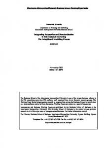
of which stem from the fact that a program’s data objects are not easily identifiable. Example 1.2.1 The program shown below will be used as an example to describe the ideas. The program initializes all elements of array pts[5] and returns pts[0].y. The x-members of each element are initialized with the value of the global variable a and the y-members are initialized with the value of global variable b. The initial values of the global variables a and b are 1 and 2, respectively. The disassembly is also shown. By convention, esp is the stack pointer in the x86 architecture. Instruction 1 allocates space for the locals of main on the stack. Fig. 1.2 shows how the variables are laid out in the activation record of main. Note that there is no space for variable i in the activation record because the compiler promoted i to register edx. Similarly, there is no space for pointer p because the compiler promoted it to register eax.
11 typedef struct { int x,y; } Point; int a = 1, b = 2; int main(){ int i, *py; Point pts[5], *p; py = &pts[0].y; p = &pts[0]; for(i = 0; i < 5; ++i) { p->x = a; p->y = b; p += 8; } return *py; }
1 2 3 4 5 6 7 L1: 8 9 10 11 12 13 14 15 16
proc main sub esp, 44 lea eax, [esp+8] mov [esp+0], eax mov ebx, [4] mov ecx, [8] mov edx, 0 lea eax,[esp+4] mov [eax], ebx mov [eax+4],ecx add eax, 8 inc edx cmp edx, 5 jl L1 mov edi, [esp+0] mov eax, [edi] add esp, 44 retn
; ;Allocate locals ;t1 = &pts[0].y ;py = t1 ;ebx = a ;ecx = b ;i = 0 ;p = &pts[0] ;p->x = a ;p->y = b ;p += 8 ;i++ ; ;(i < 5)?L1:exit loop ;t2 = py ;set return value (*t2) ;Deallocate locals ;
Instructions L1 through 12 correspond to the for-loop in the C program. Instruction L1 updates the x-members of the array elements, and instruction 8 updates the y-members. Instructions 13 and �
14 correspond to initializing the return value for main.
ret-addr pts[4].y pts[4].x
... pts[0].y pts[0].x py
0 -4 -8 -32 -36 -40 -44
Figure 1.2 Layout of the activation record for procedure main in Ex.1.2.1.
1.2.1
No Debugging/Symbol-Table Information
For many kinds of potentially malicious programs (including most COTS products, viruses, and worms), debugging information is entirely absent; for such situations, an alternative source of information about variable-like entities is needed. In any case, even if it is present, it cannot be relied upon. For this reason, the techniques that are developed to recover IR from an executable should not rely on symbol-table and debugging information being present.
12
1.2.2
Lack Of Variable-like Entities
When analyzing executables, it is difficult to track the flow of data through memory. Sourcecode-analysis tools track the flow of data through variables, which provide a finite abstraction of the address space of the program. However, in executables, as is evident from the disassembly in Ex.1.2.1, memory is accessed either directly—by specifying an absolute address—or indirectly— through an address expression of the form “[base + index × scale + offset]”, where base and index are registers, and scale and offset are integer constants. Therefore, one option is to track the contents of each memory-location in the program. However, with the large address spaces of today’s machines, it is infeasible to keep track statically of the contents of each memory address during the analysis. Without symbol-table and debugging information, a set of variable-like entities has to be inferred.
1.2.3
Information About Memory-Access Expressions
Information about memory-access expressions is a crucial requirement for any tool that works on executables. There has been work in the past on analysis techniques to obtain such information. However, they are either overly-conservative or unsound in their treatment of memory accesses. Let us consider the problem of determining data dependences between instructions in executables. An instruction i1 is data dependent on another instruction i2 if i1 reads the data that i2 writes. For instance, in Ex.1.2.1, instruction 14 is data dependent on instruction 8 because instruction 8 writes to pts[0].y and instruction 14 reads from pts[0].y. On the other hand, instruction 14 is not data dependent on instruction L1. The alias-analysis algorithm proposed by Debray et al. [45] assumes that any memory write can affect any other memory read. Therefore, their algorithm reports that instruction 14 is data dependent on both L1 and 8, i.e., it provides an overly-conservative treatment of memory operations, which can result in a lot of false positives. On the other hand, Cifuentes et al. [34] use heuristics to determine if two memory operands are aliases of one another, and hence may fail to identify the data dependence between instruction 8 and instruction 14. Obtaining information about memory-access operations in an executable is difficult because
13 • While some memory operations use explicit memory addresses in the instruction (easy), others use indirect addressing via address expressions (difficult). • Arithmetic on addresses is pervasive. For instance, even when the value of a local variable is loaded from its slot in an activation record, address arithmetic is performed—as is illustrated in instructions 2, 7 and 13 in Ex.1.2.1. • There is no notion of type at the hardware level, so address values cannot be distinguished from integer values. For instance, in Ex.1.2.1, 8 is used as an address in instruction 5 and as an integer in instruction 9. • Memory accesses do not have to be aligned, so word-sized address values could potentially be cobbled together from misaligned reads and writes. • Moreover, it is challenging to obtain reasonable information about the heap. Simple abstractions for the heap, such as assuming one summary node per malloc site [8, 105, 42] provide little useful information about the heap when applied to executables. Complex shape abstractions [100] cannot be applied to executables due to scalability reasons. My work has developed new techniques for analyzing memory accesses in executables that address these challenges, recover interesting information about memory accesses, and have a cost that is acceptable, at least for certain applications.
1.3
CodeSurfer/x86: A Tool for Analyzing Executables Along with GrammaTech, Inc., I have been developing a tool called CodeSurfer/x86 that can
be used for analyzing executables. CodeSurfer/x86 makes use of both IDAPro [67], a disassembly toolkit, and GrammaTech’s CodeSurfer system [36], a toolkit for building program-analysis and inspection tools. Fig. 1.3 shows the various components of CodeSurfer/x86. This section sketches how these components are combined in CodeSurfer/x86. An x86 executable is first disassembled using IDAPro. In addition to the set of control-flow graphs for the executable, IDAPro also provides access to the following information: (1) procedure
14 boundaries, (2) calls to library functions (identified using an algorithm called the Fast Library Identification and Recognition Technology (FLIRT) [53]), and (3) statically known memory addresses and offsets. IDAPro provides access to its internal resources via an API that allows users to create plug-ins to be executed by IDAPro. GrammaTech created a plug-in to IDAPro, called the Connector, that creates data structures to represent the information obtained from IDAPro. The IDAPro/Connector combination is also able to create the same data structures for dynamically linked libraries, and to link them into the data structures that represent the program itself. This infrastructure permits whole-program analysis to be carried out—including analysis of the code for all library functions that are called. The information that is obtained from IDAPro is incomplete in several ways: • IDAPro uses heuristics to resolve indirect jumps. Consequently, it may not resolve all indirect jumps correctly, i.e., it may not find all possible successors to an indirect jump and in some cases it might even identify incorrect successors. Therefore, the control-flow graph that is constructed from IDAPro might be incorrect/incomplete. Similarly, IDAPro might not resolve some indirect calls correctly. Therefore, a call graph created from IDAPro-supplied information is also incomplete/incorrect. • IDAPro does not provide a safe estimate of what memory locations are used and/or modified by each instruction in the executable. Such information is important for tools that aid in program understanding or bug finding. Because the information from IDAPro is incorrect/incomplete, it is not suitable as an IR for automated analysis. Based on the data structures in the Connector, I have developed Value-Set Analysis (VSA), a static-analysis algorithm that augments and corrects the information provided by IDAPro in a safe way. Specifically, it provides the following information: (1) an improved set of control-flow graphs (w/ indirect jumps resolved), (2) an improved call graph (w/ indirect calls resolved), (3) a set of variable-like entities called a-locs, (4) values held by a-locs at each point in the program (including possible address values that they may hold), and, (5) used, killed, and
15 Value added beyond IDA Pro IDA Pro Binary
Parse Binary Build CFGs
Security Analyzers Connector
CodeSurfer
Value-set Analysis
Build SDG Browse
Decompiler Binary Rewriter User Scripts
Initial estimate of • code vs. data • procedures • call sites • malloc sites
• fleshed-out CFGs • fleshed-out call graph • used, killed, may-killed variables for CFG nodes • points-to sets • reports of violations
Figure 1.3 Organization of CodeSurfer/x86. possibly-killed a-locs for CFG nodes. This information is emitted in a format that is suitable for CodeSurfer. CodeSurfer takes in this information and builds its own collection of IRs, consisting of abstractsyntax trees, control-flow graphs, a call graph, and a system dependence graph (SDG). An SDG consists of a set of program dependence graphs (PDGs), one for each procedure in the program. A vertex in a PDG corresponds to a construct in the program, such as a statement or instruction, a call to a procedure, an actual parameter of a call, or a formal parameter of a procedure. The edges correspond to data and control dependences between the vertices [52]. The PDGs are connected together with interprocedural edges that represent control dependences between procedure calls and entries, and data dependences between actual parameters and formal parameters/return values. Dependence graphs are invaluable for many applications, because they highlight chains of dependent instructions that may be widely scattered through the program. For example, given an instruction, it is often useful to know its data-dependence predecessors (instructions that write to locations read by that instruction) and its control-dependence predecessors (control points that may affect whether a given instruction gets executed). Similarly, it may be useful to know for a given instruction its data-dependence successors (instructions that read locations written by that
16 instruction) and control-dependence successors (instructions whose execution depends on the decision made at a given control point). CodeSurfer provides access to the IR through a Scheme API, which can be used to build further tools for analyzing executables.
1.4
The Scope of Our Work Analyzing executables directly is difficult and challenging; one cannot expect to design algo-
rithms that handle arbitrary low-level code. Therefore, a few words are in order about the goals, capabilities, and assumptions underlying our work: • Given an executable as input, the goal is to check whether the executable conforms to a “standard” compilation model—i.e., a runtime stack is maintained; activation records (ARs) are pushed on procedure entry and popped on procedure exit; each global variable resides at a fixed offset in memory; each local variable of a procedure f resides at a fixed offset in the ARs for f ; actual parameters of f are pushed onto the stack by the caller so that the corresponding formal parameters reside at fixed offsets in the ARs for f ; the program’s instructions occupy a fixed area of memory, are not self-modifying, and are separate from the program’s data. If the executable does conform to this model, the system will create an IR for it. If it does not conform, then one or more violations will be discovered, and corresponding error reports will be issued (see Sect. 3.8). We envision CodeSurfer/x86 as providing (i) a tool for security analysis, and (ii) a general infrastructure for additional analysis of executables. Thus, in practice, when the system produces an error report, a choice is made about how to accommodate the error so that analysis can continue (i.e., the error is optimistically treated as a false positive), and an IR is produced; if the user can determine that the error report is indeed a false positive, then the IR is valid. • The analyzer does not care whether the program was compiled from a high-level language, or hand-written in assembly. In fact, some pieces of the program may be the output from a
17 compiler (or from multiple compilers, for different high-level languages), and others handwritten assembly. • In terms of what features a high-level-language program is permitted to use, CodeSurfer/x86 is capable of recovering information from programs that use global variables, local variables, pointers, structures, arrays, heap-allocated storage, objects from classes (and subobjects from subclasses), pointer arithmetic, indirect jumps, recursive procedures, and indirect calls through function pointers (but not runtime code generation or self-modifying code). • Compiler optimizations often make VSA less difficult, because more of the computation’s critical data resides in registers, rather than in memory; register operations are more easily deciphered than memory-access operations. The analyzer is also capable of dealing with optimizations such as tail calls and tail recursion. • The major assumption that we make is that IDAPro is able to disassemble a program and build an adequate collection of preliminary IRs for it. Even though (i) the CFG created by IDAPro may be incomplete due to indirect jumps, and (ii) the call-graph created by IDAPro may be incomplete due to indirect calls, incomplete IRs do not trigger error reports. Both the CFG and the call-graph will be fleshed out according to information recovered during the course of VSA (see Sect. 3.6). In fact, the relationship between VSA and the preliminary IRs created by IDAPro is similar to the relationship between a points-to-analysis algorithm in a C compiler and the preliminary IRs created by the C compiler’s front end. In both cases, the preliminary IRs are fleshed out during the course of analysis. Specifically, we are not able to deal with the following issues: • We are not able to handle executables that modify the code section on-the-fly, i.e., executables with self-modifying code. When it is applied for such executables, our IR-recovery algorithm will uncover evidence that the executable might modify the code section, and will notify the user of the possibility.
18 • Our algorithms are capable of handling executables that contain certain kinds of obfuscations, such as instruction reordering, garbage insertion, register renaming, memory-access reordering, etc. We cannot deal with executables that use obfuscations such as unpacking/encryption; however, our techniques would be useful when applied to a memory snapshot after unpacking has been completed. Our algorithm also relies on the disassembly layer of the system to identify procedure calls and returns, which is challenging in the face of some obfuscation techniques. Even though we are not able to tackle such issues, the techniques that we have developed remain valuable (from the standpoint of what they can provide to a security analyst), and represent a significant advance over the prior state of the art.
1.5
Contributions and Organization of the Dissertation The specific technical contributions of our work, along with the organization of the dissertation,
are summarized below: In Ch. 2, we present an abstract memory model that is suitable for analyzing executables. The following concepts form the backbone of our abstract memory model: (1) memory-regions, and (2) variable-like entities referred to as a-locs. In Ch. 3, we present Value-Set Analysis (VSA), a combined pointer-analysis and numericanalysis algorithm based on abstract interpretation [40], which provides useful information about memory accesses in an executable. In particular, at each program point, VSA provides information about the contents of registers that appear in an indirect memory operand; this permits VSA to determine the addresses that are potentially accessed, which, in turn, permits it to determine the potential effects of an instruction that contains indirect memory operands on the state of memory. VSA is thus capable of dealing with operations that read from or write to memory, unlike previous techniques which either ignore memory operations altogether [45] or treat memory operations in an unsound manner [33, 34, 35].
19 In Ch. 4, we present the abstract domain used during VSA. The VSA domain is based on two’scomplement arithmetic, as opposed to many numeric abstract domains, such as the interval domain [39] and the polyhedral domain [60], which use unbounded integers or unbounded rationals. Using a domain based on two’s-complement arithmetic is important to ensure soundness when analyzing programs (either as an executable or in source-code form) in the presence of integer overflows. In Ch. 5, we present an abstract-interpretation-based algorithm that combines VSA and Aggregate Structure Identification (ASI) [93] to recover variable-like entities (the a-locs of our abstract memory model) for the executable. ASI is an algorithm that infers the substructure of aggregates used in a program based on how the program accesses them. On average, our technique is successful in identifying correctly over 88% of the local variables and over 89% of the fields of heap-allocated objects. In contrast, previous techniques, such as the one used in the IDAPro disassembler, recovered 83% of the local variables, but 0% of the fields of heap-allocated objects. In Ch. 6, we present an abstraction of heap-allocated storage referred to as recency-abstraction. Recency-abstraction is somewhere in the middle between the extremes of one summary node per malloc site [8, 42, 105] and complex shape abstractions [100]. In particular, recency-abstraction enables strong updates to be performed in many cases, and at the same time, ensures that the results are sound. Using recency-abstraction, we were able to resolve, on average, 60% of the virtual-function calls in executables that were obtained by compiling C++ programs. In Ch. 7, we present several techniques that improve the precision of the basic VSA algorithm presented in Ch. 3. All of the techniques described in Chapters 2 through 7 are incorporated in the tool that we built for analyzing Intel x86 executables, called CodeSurfer/x86. In Ch. 8, we present our experience with using CodeSurfer/x86 to find bugs in Windows devicedriver executables. We used CodeSurfer/x86 to analyze device-driver executables without the benefit of either source code or symbol-table/debugging information. We were able to find known bugs (that had been discovered by source-code analysis tools), along with useful error traces, while having a low false-positive rate. We discuss related work in Ch. 9, and present our conclusions in Ch. 10.
20
Chapter 2 An Abstract Memory Model One of the several obstacles in IR recovery is that a program’s data objects are not easily identifiable in an executable. Consider, for instance, a data dependence from statement a to statement b that is transmitted by write/read accesses on some variable x. When performing source-code analysis, the programmer-defined variables provide us with convenient compartments for tracking such data manipulations. A dependence analyzer must show that a defines x, b uses x, and there is an x-def-free path from a to b. However, in executables, memory is accessed either directly—by specifying an absolute address—or indirectly—through an address expression of the form “[base + index × scale + offset]”, where base and index are registers, and scale and offset are integer constants. It is not clear from such expressions what the natural compartments are that should be used for analysis. Because executables do not have intrinsic entities that can be used for analysis (analogous to source-level variables), a crucial step in the analysis of executables is to identify variable-like entities. If debugging information is available (and trusted), this provides one possibility; however, even if debugging information is available, analysis techniques have to account for bit-level, byte-level, word-level, and bulk-memory manipulations performed by programmers (or introduced by the compiler) that can sometimes violate variable boundaries [9, 80, 94]. If a program is suspected of containing malicious code, even if debugging information is present, it cannot be entirely relied upon. For these reasons, it is not always desirable to use debugging information—or at least to rely on it alone—for identifying a program’s data objects. (Similarly, past work on source-code analysis has shown that it is sometimes valuable to ignore information available in declarations and infer replacement information from the actual usage patterns found in the code [48, 86, 93, 102, 112].)
21 In this chapter, we present an abstract memory model for analyzing executables.
2.1
Memory-Regions A simple model for memory is to consider memory as an array of bytes. Writes (reads) in
this trivial memory model are treated as writes (reads) to the corresponding element of the array. However, there are some disadvantages in such a simple model: • It may not be possible to determine specific address values for certain memory blocks, such as those allocated from the heap via malloc. For the analysis to be sound, writes to (reads from) such blocks of memory have to be treated as writes to (reads from) any part of the heap, which leads to imprecise (and mostly useless) information about memory accesses. • The runtime stack is reused during each execution run; in general, a given area of the runtime stack will be used by several procedures at different times during execution. Thus, at each instruction a specific numeric address can be ambiguous (because the same address may belong to different Activation Records (ARs) at different times during execution): it may denote a variable of procedure f, a variable of procedure g, a variable of procedure h, etc. (A given address may also correspond to different variables of different activations of f.) Therefore, an instruction that updates a variable of procedure f would have to be treated as possibly updating the corresponding variables of procedures g, h, etc., which also leads to imprecise information about memory accesses. To overcome these problems, we work with the following abstract memory model [11]. Although in the concrete semantics the activation records for procedures, the heap, and the memory area for global data are all part of one address space, for the purposes of analysis, we separate the address space into a set of disjoint areas, which are referred to as memory-regions (see Fig. 2.1). Each memory-region represents a group of locations that have similar runtime properties: in particular, the runtime locations that belong to the ARs of a given procedure belong to one memoryregion. Each (abstract) byte in a memory-region represents a set of concrete memory locations. For a given program, there are three kinds of regions: (1) the global-region, for memory locations that
22 ... AR of G
...
AR of F
AR of F
... AR of G AR of G
GLOBAL DATA GLOBAL DATA
Runtime Address Space
Memory Regions
Figure 2.1 Abstract Memory Model hold initialized and uninitialized global data, (2) AR-regions, each of which contains the locations of the ARs of a particular procedure, and (3) malloc-regions, each of which contains the locations allocated at a particular malloc site. We do not assume anything about the relative positions of these memory-regions. For an n-bit architecture, the size of each memory-region in the abstract memory model is 2n . For each region, the range of offsets within the memory-region is [−2n−1 , 2n−1 − 1]. Offset 0 in an AR-region represents all concrete addresses at which an activation record for the procedure is created. Offset 0 in a malloc-region represents all concrete addresses at which the heap block is allocated. For the global-region, offset 0 represents the concrete address 0. The analysis treats all data objects, whether local, global, or in the heap, in a fashion similar to the way compilers arrange to access variables in local ARs, namely, via an offset. We adopt this notion as part of our abstract semantics: an abstract memory address is represented by a pair: (memory-region, offset). By convention, esp is the stack pointer in the x86 architecture. On entry to a procedure P, esp points to the top of the stack, where the new activation record for P is created. Therefore, in our abstract memory model, esp holds abstract address (AR P, 0) on entry to procedure P, where AR P is the activation-record region associated with procedure P. Similarly, because malloc returns the starting address of an allocated block, the return value for malloc (if allocation is successful)
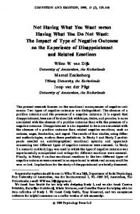
23 is the abstract address (Malloc n, 0), where Malloc n is the memory-region associated with the call-site on malloc.1 Example 2.1.1 Fig. 2.2(b) shows the memory-regions for the program in Ex.1.2.1. There is a single procedure, and hence two regions: one for global data and one for the AR of main. Furthermore, the abstract address of local variable py is the pair (AR main,-44) because it is at offset -44 with respect to the AR’s creation point. Similarly, the abstract address of global variable b is (Global,8).
2.2
�
Abstract Locations (A-Locs) Memory-regions provide a way of summarizing information about a set of concrete addresses,
but they alone do not provide an analog of the source-level variables used in source-code analysis. As pointed out earlier, executables do not have intrinsic entities like source-code variables that can be used for analysis; therefore, the next step is to recover variable-like entities from the executable. We refer to such variable-like entities as a-locs (for “abstract locations”). Heretofore, the state of the art in recovering variable-like entities is represented by IDAPro [67], a commercial disassembly toolkit. IDAPro’s algorithm is based on the observation that the data layout of the program is established before generating the executable; therefore, accesses to global variables appear as “[absolute-address]”, and accesses to local variables appear as “[esp + offset]” or “[ebp − offset]” in the executable. IDAPro identifies such statically-known absolute addresses, esp-based offsets, and ebp-based offsets in the program, and treats the set of locations in between two such absolute addresses or offsets to be one a-loc. That is, IDAPro recovers variables based on purely local techniques.2 We refer to IDAPro’s algorithm as the Semi-Na¨ıve algorithm. Let us look at the a-locs identified by Semi-Na¨ıve algorithm for the program in Ex.1.2.1. 1
CodeSurfer/x86 actually uses an abstraction of heap-allocated storage that involves more than one memory-region per call-site on malloc [12]. This is discussed in Ch. 6 2 IDAPro does incorporate a few global analyses, such as one for determining changes in stack height at call-sites. However, the techniques are ad-hoc and based on heuristics.
24 FormalGuard
231-1 4
ret-addr
ret-addr pts[4].y pts[4].x
... pts[0].y pts[0].x py
0
0 -4 -8
mem_8 var_36
8 mem_4 4
-36
-32
var_40
-36 -40 -44
var_44 LocalGuard
Global Region
-40 -44 -231
AR_main
(a)
(b)
Figure 2.2 (a) Layout of the activation record for procedure main in Ex.1.2.1; (b) a-locs identified by IDAPro. Global a-locs
In Ex.1.2.1, instructions “mov ebx, [4]” and “mov ecx,[8]” have direct mem-
ory operands, namely, [4] and [8]. IDAPro identifies these statically-known absolute addresses as the starting addresses of global a-locs and treats the locations between these addresses as one a-loc. Consequently, IDAPro identifies addresses 4..7 as one a-loc, and the addresses 8..11 as another a-loc. Therefore, we have two a-locs: mem 4 (for addresses 4..7) and mem 8 (for addresses 8..11). (Note that an executable can have separate sections for read-only data. The global a-locs in such sections are marked as read-only a-locs.) Local a-locs Local a-locs are determined on a per-procedure basis as follows. At each instruction in the procedure, IDAPro computes the difference between the value of esp (or ebp) at that point and the value of esp at procedure entry. These computed differences are referred to as sp delta.3 After computing sp delta values, IDAPro identifies all esp-based indirect operands in the procedure. In Ex.1.2.1, instructions “lea eax, [esp+8]”, “mov [esp+0], eax”, “lea eax, [esp+4]”, and “mov edi, [esp+0]” have esp-based indirect operands. Recall that on entry to procedure main, esp contains the abstract address (AR main, 0). Therefore, for every 3
Note that when computing the sp delta values, IDAPro uses heuristics to identify changes to esp (or ebp) at procedure calls and instructions that access memory. Therefore, the sp delta values may be incorrect (i.e., unsound). Consequently, the layout obtained by IDAPro for an AR may be incorrect. However, this is not an issue for our algorithms (such as the Value-Set Analysis algorithm discussed in Ch. 3) that use the a-locs identified by IDAPro; all our algorithms have been designed to be resilient to IDAPro having possibly provided an incorrect layout for an AR.
25 esp/ebp-based operand, the computed sp delta values give the corresponding offset in AR main. For instance, [esp+0], [esp+4], and [esp+8] refer to offsets -44, -40 and -36 respectively in AR main. This gives rise to three local a-locs: var 44, var 40, and var 36. Note that var 44 corresponds to all of the source-code variable py. In contrast, var 40 and var 36 correspond to disjoint segments of array pts[]: var 40 corresponds to program variable pts[0].x; var 36 corresponds to the locations of program variables pts[0].y, p[1..4].x, and p[1..4].y. In addition to these a-locs, an a-loc for the return address is also defined; its offset in AR main is 0. In addition to the a-locs identified by IDAPro, two more a-locs are added:(1) a FormalGuard that spans the space beyond the topmost a-loc in the AR-region, and (2) a LocalGuard that spans the space below the bottom-most a-loc in the AR-region. FormalGuard and LocalGuard delimit the boundaries of an activation record. Therefore, a memory write to FormalGuard or LocalGuard represents a write beyond the end of an activation record. Heap a-locs
In addition to globals and locals, we have one a-loc per heap-region. There are no
heap a-locs for Ex.1.2.1 because it does not access the heap. Registers In addition to the global, heap, and local a-locs, registers are also considered to be a-locs. Once the a-locs are identified, we also maintain a mapping from a-locs to (rgn, off, size) triples, where rgn represents the memory-region to which the a-loc belongs, off is the starting offset of the a-loc in rgn, and size is the size of the a-loc. The starting offset of an a-loc a in a region rgn is denoted by offset(rgn, a). For Ex.1.2.1, offset(AR main,var 40) is -40 and offset(Global, mem 4) is 4. This mapping is used to interpret memory-dereferencing operations as described in Sect. 3.4.
26
Chapter 3 Value-Set Analysis (VSA) As described in Sect. 1.2, one of the significant obstacles in analyzing executables is that it is very difficult to obtain useful information about how the program manipulates data in memory. This chapter describes the value-set analysis (VSA) algorithm, which provides useful information about memory accesses in an executable. VSA is a combined numeric-analysis and pointeranalysis algorithm that determines a safe approximation of the set of numeric values or addresses that each register and a-loc holds at each program point. In particular, at each program point, VSA provides information about the contents of registers that appear in an indirect memory operand; this permits it to determine the addresses (and hence the a-locs) that are potentially accessed, which, in turn, permits it to determine the potential effects on the state of an instruction that contains an indirect memory operand. The problem that VSA addresses has similarities with the pointer-analysis problem that has been studied in great detail for programs written in high-level languages. For each variable (say v), pointer analysis determines an over-approximation of the set of variables whose addresses v can hold. Similarly, VSA determines an over-approximation of the set of addresses that a register or a memory location holds at each program point. For instance, VSA determines that at instruction L1 in Ex.1.2.1 eax holds offsets −40, −32, −24, . . . , −8 in the activation record of procedure main, which corresponds to the addresses of field x of the elements of array pts[0..4]. On the other hand, VSA also has some of the flavor of numeric static analyses, where the goal is to over-approximate the integer values that each variable can hold; in addition to information about addresses, VSA determines an over-approximation of the set of integer values that each data
27 object can hold at each program point. For instance, VSA determines that at instruction L1, edx holds numeric values in the range [0, 4]. A key feature of VSA is that it tracks integer-valued and address-valued quantities simultaneously. This is crucial for analyzing executables because numeric values and addresses are indistinguishable at runtime. Moreover, unlike earlier algorithms [33, 34, 35, 45], VSA takes into account data manipulations involving memory locations also. VSA is based on abstract interpretation [40], where the aim is to determine the possible states that a program reaches during execution, but without actually running the program on specific inputs. Abstract-interpretation techniques explore the program’s behavior for all possible inputs and all possible states that the program can reach. To make this feasible, the program is run in the aggregate, i.e., on descriptors that represent collections of memory configurations. The universal set of descriptors used in abstract interpretation is referred to as an abstract domain. VSA is a flow-sensitive, context-sensitive, interprocedural, abstract-interpretation algorithm (parameterized by call-string length [101]) that is based on an independent-attribute abstract domain. Informally, an element in the abstract domain for VSA associates each a-loc (including registers) in the executable with an (abstract) set of memory addresses and numeric values. That is, an element in the abstract domain represents a set of concrete (i.e., run-time) states of a program. In the rest of this chapter, we formalize the VSA domain and describe the value-set analysis (VSA) algorithm in detail. This chapter is organized as follows. Sects. 3.1, 3.2, and 3.3 describe the VSA domain. Sects. 3.4, 3.5, and 3.7 describe several variations of the VSA algorithm. Sect. 3.6 describes how VSA handles indirect jumps and indirect calls. Sect. 3.8 discusses soundness issues. CodeSurfer/x86 uses the context-sensitive VSA algorithm described in Sect. 3.7. Algorithms described in Sects. 3.4 and 3.5 are simply used to present the core ideas that are needed to describe the context-sensitive VSA algorithm.
28
3.1
Value-Set A value-set represents a set of memory addresses and numeric values. Recall from Sect. 2.1
that every memory address is a pair (memory-region, offset). Therefore, a set of memory addresses can be represented by a set of tuples of the form (rgni 7→ {oi1 , oi2 , ..., oini }). A value-set uses a k-bit strided-interval (SI) [94] to represent the set of offsets in each memory region. A k-bit strided interval s[l, u] represents a set of integers {i ∈ [−2k−1 , 2k−1 − 1] | l ≤ i ≤ u, i ≡ l(mod s)}. • s is called the stride. • [l, u] is called the interval. • 0[l, l] represents the singleton set {l}. We also call ⊥ a strided interval; it denotes the empty set of offsets. Consider the set of addresses S = {(Global 7→ {1, 3, 5, 9}), (AR main 7→ {−48, −40})}. The value-set for S is the set {(Global 7→ 2[1, 9]), (AR main 7→ 8[−48, −40])}. Note that the value-set for S is an over-approximation; the value-set includes the global address 7, which is not an element of S. For conciseness, a value-set will be shown as an r-tuple of SIs, where r is the number of memory-regions for the executable. By convention, the first component of the r-tuple represents addresses in the Global memory-region. Using the concise notation, the value-set for S is the 2-tuple, (2[1, 9], 8[−48, −40]). A value-set is capable of representing a set of memory addresses as well as a set of numeric values. For instance, the 2-tuple (2[1, 9], ⊥) denotes the set of numeric values {1, 3, 5, 7, 9} as well as the set of addresses {(Global, 1), (Global, 3), . . . , (Global, 9)}; the 2-tuple (⊥, 8[−48, −40]) represents the set of addresses {(AR main, −48), (AR main, −40)}. This is a crucial requirement for analyzing executables because numbers and addresses are indistinguishable in an executable. Advantages of Strided Intervals for Analysis of Executables
We chose to use SIs instead of
ranges because, in our context, it is important for the analysis to discover alignment and stride information so that it can interpret indirect-addressing operations that implement either (i) fieldaccess operations in an array of structs, or (ii) pointer-dereferencing operations.
29 Let *a denote the contents of a-loc a. When the contents of a-loc a is not aligned with the boundaries of other a-locs, a memory access *a can fetch portions of two a-locs; similarly, a write to *a can overwrite portions of two a-locs. Such operations can be used to forge new addresses. For instance, suppose that the address of a-loc x is 1000, the address of a-loc y is 1004, and the contents of a is 1001. Then *a (as a 4-byte fetch) would retrieve 3 bytes of x and 1 byte of y. This issue motivated the use of SIs because SIs are capable of representing certain non-convex sets of integers, and ranges (alone) are not. Suppose that the contents of a is the set {1000, 1004}; then *a (as a 4-byte fetch) would retrieve all of x (and none of y) or all of y (and none of x). The range [1000, 1004] includes the addresses 1001, 1002, and 1003, and hence *[1000, 1004] (as a 4-byte fetch) could result in a forged address. However, because VSA is based on SIs, {1000, 1004} is represented exactly, as the SI 4[1000, 1004]. If VSA were based on range information rather than SIs, it would either have to try to track segments of (possible) contents of data objects, or treat such dereferences conservatively by returning >vs , thereby losing track of all information. The Value-Set Abstract Domain
Value-sets form a lattice. Informal descriptions of a few 32-bit
value-set operators are given below. Ch. 4 describes the operations on value-sets in detail. • (vs1 vvs vs2 ): Returns true if the value-set vs1 is a subset of vs2 , false otherwise. • (vs1 uvs vs2 ): Returns the meet (intersection) of value-sets vs1 and vs2 . • (vs1 tvs vs2 ): Returns the join (union) of value-sets vs1 and vs2 . • (vs1 ∇vs vs2 ): Returns the value-set obtained by widening [39] vs1 with respect to vs2 , e.g., if vs1 = (4[40, 44]) and vs2 = (4[40, 48]), then (vs1 ∇vs vs2 ) = (4[40, 231 − 3]). Note that the upper bound for the interval in the result is 231 − 3 (and not 231 − 1) because 231 − 3 is the maximum positive value that is congruent to 40 modulo 4. • (vs +vs c): Returns the value-set obtained by adjusting all values in vs by the constant c, e.g., if vs = (4, 4[4, 12]) and c = 12, then (vs +vs c) = (16, 4[16, 24]).
30 • ∗(vs, s): Returns a pair of sets (F, P ). F represents the set of “fully accessed” a-locs: it consists of the a-locs that are of size s and whose starting addresses are in vs. P represents the set of “partially accessed” a-locs: it consists of (i) a-locs whose starting addresses are in vs but are not of size s, and (ii) a-locs whose addresses are in vs but whose starting addresses and sizes do not meet the conditions to be in F . • RemoveLowerBounds(vs): Returns the value-set obtained by setting the lower bound of each component SI to −231 .
For example, if vs = ([0, 100], [100, 200]), then
RemoveLowerBounds(vs)= ([−231 , 100], [−231 , 200]). • RemoveUpperBounds(vs): Similar to RemoveLowerBounds, but sets the upper bound of each component to 231 − 1.
3.2
Abstract Environment (AbsEnv) AbsEnv (for “abstract environment”) is the abstract domain used during VSA to represent a
set of concrete stores that arise at a given program point. This section formalizes AbsEnv. Let Proc denote the set of memory-regions associated with procedures in the program; AllocMemRgn denote the set of memory-regions associated with heap-allocation sites; Global denote the memory-region associated with the global data area; and a-locs[R] denote the a-locs that belong to memory-region R. We work with the following basic domains: MemRgn = {Global} ∪ Proc ∪ AllocMemRgn ValueSet = MemRgn → StridedInterval⊥ AlocEnv[R] = a-locs[R] → ValueSet Flag = {CF, ZF, SF, PF, AF, OF} Flag represents the set of x86 flags. An x86 flag is either set to T RUE or FALSE at runtime. To represent multiple possible Boolean values, we use the abstract domain Bool3: Bool3 = {FALSE, M AYBE, T RUE}. In addition to the Booleans FALSE and T RUE, Bool3 has a third value, M AYBE, which means “may be FALSE or may be T RUE”.
31 AbsEnv maps each region R to its corresponding AlocEnv[R], each register to a ValueSet, and each Flag to a Bool3: (register → ValueSet) × (Flag → Bool3) AbsEnv = × ({Global} → AlocEnv[Global]) × (Proc → AlocEnv[Proc]⊥ ) × (AllocMemRgn → AlocEnv[AllocMemRgn]⊥ ) That is, an AbsEnv represents a set of concrete states that arise at a program point on a set of runs of a program. Because the values of read-only locations cannot change during program execution, read-only a-locs are not included in AbsEnv for efficiency. In the above definitions, ⊥ is used to denote a partial map. For instance, a ValueSet may not contain offsets in some memory-regions. Similarly, in AbsEnv, a procedure P whose activation record is not on the stack does not have an AlocEnv[P]. We use the following notational conventions: • Given a memory a-loc or a register a-loc a and ae ∈ AbsEnv, ae[a] refers to the ValueSet for a-loc a in ae. • Given vs ∈ ValueSet and r ∈ MemRgn, vs[r] refers to the strided interval for memoryregion r in vs. • Given f ∈ Flag and ae ∈ AbsEnv, ae[f] refers to the Bool3 for flag f in ae.
3.3
Representing Abstract Stores Efficiently To represent the abstract store at each program point efficiently, we use applicative dictionaries,
which provide a space-efficient representation of a collection of dictionary values when many of the dictionary values have nearly the same contents as other dictionary values in the collection [96, 84].
32 Applicative dictionaries can be implemented using applicative balanced trees, which are standard balanced trees on which all operations are carried out in the usual fashion, except that whenever one of the fields of an interior node M would normally be changed, a new node M 0 is created that duplicates M , and changes are made to the fields of M 0 . To be able to treat M 0 as the child of parent(M ), it is necessary to change the appropriate child-field in parent(M ), so a new node is created that duplicates parent(M ), and so on, all the way to the root of the tree. Thus, new nodes are introduced for each of the original nodes along the path from M to the root of the tree. Because an operation that restructures a standard balanced tree may modify all of the nodes on the path to the root anyway, and because a single operation on a standard balanced tree that has n nodes takes at most O(log n) steps, the same operation on an applicative balanced tree introduces at most O(log n) additional nodes and also takes at most O(log n) steps. The new tree resulting from the operation shares the entire structure of the original tree except for the nodes on a path from M 0 to the root, plus at most O(log n) other nodes that may be introduced to maintain the balance properties of the tree. In our implementation, the abstract stores from the VSA domain are implemented using applicative AVL trees [84]. That is, each function or partial function in a component of AbsEnv is implemented with an applicative AVL tree. The use of shared data structures to reduce the space required for program analysis has a long history; it includes applicative shared dictionaries [84, 96], shared set representations [92], and binary decision diagrams [23, 24]. Recent work that discusses efficient representations of data structures for program analysis includes [18, 78].
3.4
Intraprocedural Analysis This subsection describes an intraprocedural version of VSA. For the time being, we consider
programs that have a single procedure and no indirect jumps. To aid in explaining the algorithm, we adopt a C-like notation for program statements. We will discuss the following kinds of instructions, where R1 and R2 are two registers of the same size, c, c1 , and c2 are explicit integer constants, and
33 ≤ and ≥ represent signed comparisons: R1 = R2 + c *(R1 + c1 ) = R2 + c2
R1 ≤ c R1 ≥ R2
R1 = *(R2 + c1 ) + c2 Conditions of the two forms shown on the right are obtained from the instruction(s) that set condition codes used by branch instructions (see Sect. 3.4.2). The analysis is performed on a control-flow graph (CFG) for the procedure. The CFG consists of one node per x86 instruction, and there is a directed edge n1 →n2 between a pair of nodes n1 and n2 in the CFG if there is a flow of control from n1 to n2. The edges are labeled with the instruction at the source of the edge. If the source of an edge is a branch instruction, then the edge is labeled according to the outcome of the branch. For instance in the CFG for the program in Ex.1.2.1, the edge 12→L1 is labeled edxvs . Similarly, case 3 treats a load of a potentially forged address as a load of >vs . (Techniques for more precise handling of partial accesses to a-locs are discussed in Ch. 5.)
34 Instruction R1 = R2 + c
∗(R1 + c1 ) = R2 + c2
R1 = ∗(R2 + c1 ) + c2
R1 ≤ c
R1 ≥ R2
AbstractTransformer(in: AbsEnv): AbsEnv Let out := in and vsR2 := in[R2] out[R1] := vsR2 +vs c return out Let vsR1 := in[R1], vsR2 := in[R2], (F, P ) = ∗(vsR1 +vs c1 , s), and out := in Let Proc be the procedure containing the instruction if (|F | = 1 ∧ |P | = 0 ∧ (F has no heap a-locs or a-locs of recursive procedures)) then out[v] := vsR2 +vs c2 , where v ∈ F // Strong update else for each v ∈ F do out[v] := out[v] tvs (vsR2 +vs c2 ) // Weak update end for end if for each v ∈ P do // Set partially accessed a-locs to >vs out[v] := >vs end for return out Let vsR2 := in[R2], (F, P ) = ∗(vsR2 +vs c1 , s) and out := in if (|P | = 0) then F Let vsrhs := vs {in[v] | v ∈ F } out[R1] := vsrhs +vs c2 else out[R1] := >vs end if return out Let vsc := ([−231 , c], >si , . . . , >si ) and out := in out[R1] := in[R1] uvs vsc return out Let vsR1 := in[R1] and vsR2 := in[R2] Let vslb := RemoveUpperBounds(vsR2 ) and vsub := RemoveLowerBounds(vsR1 ) out := in out[R1] := vsR1 uvs vslb out[R2] := vsR2 uvs vsub return out
Figure 3.1 Abstract transformers for VSA. (In cases 2 and 3, s represents the size of the dereference performed by the instruction.) Given a CFG G for a procedure (without calls), the goal of intraprocedural VSA is to annotate each node n with absEnvn ∈ AbsEnv, where absEnvn represents an over-approximation of the set of memory configurations that arise at node n over all possible runs of the program. The intraprocedural version of the VSA algorithm is given in Fig. 3.2. The value of absEnventer consists of information about the initialized global variables and the initial value of the stack pointer (esp).
35 1: decl worklist: Set of Node 2: 3: proc IntraProceduralVSA() 4: worklist := {enter} 5: absEnventer := Initial values of global a-locs and esp 6: while (worklist 6= ∅) do 7: Select and remove a node n from worklist 8: m := Number of successors of node n 9: for i = 1 to m do 10: succ := GetCFGSuccessor(n, i) 11: edge amc := AbstractTransformer(n → succ, absEnvn ) 12: Propagate(succ, edge amc) 13: end for 14: end while 15: end proc 16: 17: proc Propagate(n: Node, edge amc: AbsEnv) 18: old := absEnvn 19: new := old tae edge amc 20: if (old 6= new) then 21: absEnvn := new 22: worklist := worklist ∪ {n} 23: end if 24: end proc
Figure 3.2 Intraprocedural VSA Algorithm. The AbsEnv abstract domain has very long ascending chains.1 Hence, to ensure termination, widening needs to be performed. Widening needs to be carried out at at least one edge of every cycle in the CFG; however, the edge at which widening is performed can affect the accuracy of the analysis. To choose widening edges, our implementation of VSA uses techniques from [20] (see Sect. 7.1). Example 3.4.1 This example presents the results of intraprocedural VSA for the program in Ex.1.2.1. For the program in Ex.1.2.1, the AbsEnv for the entry node of main is {esp 7→ (⊥, 0), mem 4 7→ (1, ⊥), mem 8 7→ (2, ⊥)}. Recall that instruction “L1:mov [eax], ebx” updates the x members of array pts. Instruction “14:
mov eax, [edi]” initializes the return value of main to
p[0].y. The results of the VSA algorithm at instructions L1, 8, and 14 are as follows: 1
The domain is of bounded height because strided intervals are based on 32-bit 2’s complement arithmetic. However, for a given executable, the bound is very large: each a-loc can have up to |MemRgn| SIs; hence the height is (n × |MemRgn| × 232 ), where n is the total number of a-locs.
36 Instruction L1 and 8 esp 7→ (⊥, −44) mem 4 7→ (1, ⊥) mem 8 7→ (2, ⊥) eax 7→ (⊥, 8[−40, 231 − 7]) ebx 7→ (1, ⊥) ecx 7→ (2, ⊥) edx 7→ (1[0, 4], ⊥) edi 7→ >vs var 44 7→ (⊥, −36)
Instruction 14 esp 7→ (⊥, −44) mem 4 7→ (1, ⊥) mem 8 7→ (2, ⊥) eax 7→ (⊥, 8[−40, 231 − 7]) ebx 7→ (1, ⊥) ecx 7→ (2, ⊥) edx 7→ (5, ⊥) edi 7→ (⊥, −36) var 44 7→ (⊥, −36)
That is, we have the following facts: • At instruction L1, the set of possible values for edx is {0, 1, 2, 3, 4}. At instruction 14, the only possible value for edx is 5. (Recall that edx corresponds to the loop variable i in the C program.) • At instruction L1, eax holds the following set of addresses: {(AR main, −40), (AR main, −32), . . . , (AR main, 0), . . . , (AR main, 231 − 7)} That is, at instruction L1, eax holds the addresses of the local a-locs var 40, var 36, ret-addr, and FormalGuard. (See Fig. 2.2(b) for the layout of AR main.) Therefore, instruction L1 possibly modifies var 40, var 36, ret-addr, and FormalGuard. Similarly, at instruction 8, eax+4 refers to the following set of addresses: {(AR main, −36), (AR main, −28), . . . , (AR main, 4), . . . , (AR main, 231 − 3)} Therefore, instruction 8 possibly modifies var 36 and FormalGuard. • At instruction 14, the only possible value for edi is the address (AR main, −36), which corresponds to the address of the local a-loc var 36. The value-sets obtained by the analysis can be used to discover the data dependences that exist between instructions 8 and 14. At instruction 8, the set of possibly-modified a-locs is {var 36, FormalGuard}. At instruction 14, the set of used a-locs is {var 36}. Reaching-definitions analysis based on this information reveals that instruction 14 is data dependent on instruction 8. However, reaching-definitions analysis based on the information at instruction L1 would also reveal
37 that instruction 14 is also data dependent on instruction L1, which is spurious (i.e., a false positive), because the set of actual addresses accessed at instruction L1 and instruction 14 are different. The reason for the spurious data dependence is that the Semi-Na¨ıve algorithm, described in Ch. 2, recovers too coarse a set of a-locs. For instance, for the program in Ex.1.2.1, the Semi-Na¨ıve algorithm failed to recover any information about the array pts. Ch. 5 presents an improved a-loc recovery algorithm that is capable of recovering information about arrays, fields of structs, etc., thereby reducing the number of spurious data dependences. At instruction L1, the set of possibly-modified a-locs includes ret-addr, which is the a-loc for the return address. This is because the analysis was not able to determine a precise upper bound for eax at instruction L1, although register edx has a precise upper and lower bound at instruction L1. Note that, because eax and edx are incremented in lock-step within the loop, the affine relation eax = (esp + edx × 8) + 4 holds at instruction L1. We discuss in Sect. 7.2 how the implemented system actually uses such affine relations to find precise upper or lower bounds for registers, such �
as eax, within a loop.
3.4.1
Idioms
Before applying an abstract transformer, the instruction is checked to see if it matches a pattern for which we know how to carry out abstract interpretation more precisely than if value-set arithmetic is performed directly. Some examples are given below. XOR r1,r2, when r1 = r2 = r.
The XOR instruction sets its first operand to the bitwise exclusive-
or (∧ ) of the instruction’s two operands. The idiom catches the case when XOR is used to set a register to 0; hence, the a-loc for register r is set to the value-set (0[0, 0], ⊥, . . .). TEST r1,r2, when r1 = r2 = r.
The TEST instruction computes the bitwise and (&) of its two
operands, and sets the SF, ZF, and PF flags according to the result. The idiom addresses how the value of ZF is set when the value-set of r has the form (si, ⊥, . . .):
38 T RUE if γ(si) = {0} ZF := FALSE if γ(si) ∩ {0} = ∅ M AYBE otherwise
where ‘γ’ is the concretization function for the strided-interval domain (see Defn. 4.2.1). CMP a,b or CMP b,a.
In the present implementation, we assume that an allocation always suc-
ceeds (and hence value-set analysis only explores the behavior of the system on executions in which allocations always succeed). Under this assumption, we can apply the following idiom: Suppose that k1, k2, . . . are malloc-regions, the value-set for a is (⊥, . . . , sik1 , sik2 , . . .), and the value-set for b is (0[0, 0], ⊥, . . .). Then ZF is set to FALSE.
3.4.2
Predicates for Conditional Branch Instructions
In x86 architectures, predicates used in high-level control constructs such as if, while, for, etc. are implemented using conditional branch instructions. A conditional branch instruction (say jxx TGT) evaluates a predicate involving the processor’s flags and transfers control to the target instruction (TGT) if the predicate expression is T RUE; otherwise, it transfers control to the next instruction. For instance, a jl instruction evaluates the conditional expression SF = 1, where SF is the sign flag. It is not clear from conditional expressions such as SF = 1 what the high-level predicate is. To determine the high-level predicate, it is necessary to consider the instruction that sets the processor’s flags before the conditional jump instruction is executed. In Ex.1.2.1, i < 5 is compiled down to the x86 instruction sequence (cmp edx, 5; jl L1). The cmp operation sets the processor’s flags to the result of computing the arithmetic expression edx − 5. Instruction “cmp edx, 5” sets SF to 1 iff (edx − 5 < 0), i.e., iff edx < 5. Because instruction jl is preceded by “cmp edx, 5” and jl transfers control to L1 iff SF = 1, we conclude that the instruction sequence (cmp edx, 5; jl L1) implements the high-level predicate edx < 5. High-level predicates for various instruction sequences involving conditional jump instructions are shown in Fig. 3.3.
39 cmp X, Y Flag Predicate Predicate
sub X, Y test X, Y Flag Predicate Predicate Flag Predicate Predicate Unsigned Comparisons ja,jnbe ¬CF ∧ ¬ZF X >u Y ¬CF ∧ ¬ZF X0 6= 0 ¬ZF X&Y 6= 0 jae,jnb,jnc ¬CF X ≥u Y ¬CF ? T RUE T RUE jb,jnae,jc CF X Y ¬ZF ∧ (OF ⇔ SF) X0 = 0 ¬ZF ∧ ¬SF (X&Y 6= 0) ∧ (X > 0 ∨ Y > 0) jge,jnl OF ⇔ SF X≥Y OF ⇔ SF ? ¬SF (X ≥ 0 ∨ Y ≥ 0) jl,jnge (OF ⊕ SF) Xx = a; p->y = b; p += 8; } return *py; } int main(){ Point pts[5]; return initArray(pts, 5); }
1 2 3 4 5 6 7 L1: 8 9 10 11 12 13 14 15
proc initArray sub esp, 4 lea eax, [esp+16] mov [esp+0], eax mov ebx, [4] mov ecx, [8] mov edx, 0 lea eax, [esp+12] mov [eax], ebx mov [eax+4],ecx add eax, 8 inc edx cmp edx,[esp+4] jl L1 mov edi, [esp+0] mov eax, [edi] add esp, 12
16
retn
17 18 19 20 21 22
proc main sub esp, 40 push 5 push esp call initArray add esp, 40 retn
; ;Allocate locals ;t1 = &pts[0].y ;py = t1 ;ebx = a ;ecx = b ;i = 0 ;p = &pts[0] ;p->x = a ;p->y = b ;p += 8 ;i++ ; ;(i < n)?L1:exit loop ;t2 = py ;set return value (*t2) ;Deallocate locals and ;actuals ; ; ; ;Allocate locals ;2nd actual ;1st actual ; ; ;
The memory-regions and their layout are shown in Fig. 3.4. Note that all the local variables in initArray are mapped to registers in the disassembly: i is mapped to edx, p is mapped to eax, and py is mapped to edi. Therefore, AR initArray only has the following three a-locs: the return address, formal parameter arg 0, and formal parameter arg 4.
�
41 Observation 3.5.2 In our abstract memory model, we do not assume anything about the relative positions of the memory-regions. However, at a call, it is possible to establish the relative positions of the caller’s AR-region (AR C) and the callee’s AR-region (AR X). Fig. 3.5 illustrates this idea. At runtime, AR C and AR X overlap on the stack just before a call is executed. Specifically, the abstract address (AR C, −s) in memory-region AR C corresponds to the abstract address (AR X, 4) in memory-region AR X. Therefore, the value of esp at a call refers to the abstract address (AR C, −s) or (AR X, 4). This observation about the relative positions of AR C and AR X established at a call-site is used to develop the abstract transformers for the linkage edges. For instance, at instruction 20 in Ex.3.5.1, (AR main, −48) corresponds to (AR initArray, 4). Note that the observation about the relative positions of AR main and AR initArray at instruction 20 enables us to establish a correspondence between the formal parameters arg 0 and arg 4 of AR initArray and the actual parameters ext 48 and ext 44 of AR main, respectively. (See Fig. 3.4.) This correspondence between the actuals parameters of the caller and the formal parameters of the callee is used to initialize the formal parameters in the abstract transformer for a �
call→enter edge.
...
s
AR_C
esp return address
(AR_C, 0)
(AR_C, -s) (or) (AR_X, 4)
AR_X (AR_X, 0)
... GLOBAL DATA
Figure 3.5 Relative positions of the AR-regions of the caller (C) and callee (X) at a call.
3.5.1
Abstract Transformer for call→enter Edge
The pseudo-code for the abstract transformer for the call→enter edge is shown in Fig. 3.6. Procedure CallEnterTransformer takes the current AbsEnv value at the call node as an argument and returns a new AbsEnv value for the call→enter edge. As a first step, the value-set of esp
42 1: proc CallEnterTransformer(in : AbsEnv): AbsEnv 2: Let C be the caller and X be the callee. 3: out := in 4: out[esp] := (⊥, . . . , 0, . . . , ⊥) // 0 occurs in the slot for AR X 5: for each a-loc a ∈ a-locs[AR X] do 6: Let Sa be the size of the a-loc a. 7: // Find the corresponding a-locs in AR C. 8: (F, P ) := ∗(in[esp] +vs offset(AR X, a), Sa ) 9: newa := ⊥vs 10: if (P 6= ∅) then 11: newa := >vs 12: else 13: vsactuals := tvs {in[v] | v ∈ F } 14: newa := vsactuals 15: end if 16: if X is recursive then 17: out[a] := in[a] tvs newa 18: else 19: out[a] := newa 20: end if 21: end for 22: return out 23: end proc
Figure 3.6 Transformer for call→enter edge. in the newly computed value is set to (⊥, . . . , 0, . . . , ⊥), where the 0 occurs in the slot for AR X (line [4] in Fig. 3.6). This step corresponds to changing the current AR from that of AR C to AR X. After initializing esp, for every a-loc a ∈ a-locs[AR X], the corresponding set of a-locs in the AR X is determined (line [8] of Fig. 3.6), and a new value-set for a (namely newa ) is computed (lines [6]–[15] of Fig. 3.6). (Note that line [8] of Fig. 3.6 is based on Obs. 3.5.2.) If procedure X is not recursive, the value-set for a in out is initialized to newa (line [19] of Fig. 3.6). If procedure X is recursive, a weak update is performed (line [17] of Fig. 3.6). It is necessary to perform a weak update (rather than a strong update as at line [19] of Fig. 3.6) because the AR-region for a recursive procedure (say P) represents more than one concrete instance of P’s activation record. Note that initialization of the a-locs of callee X (lines [5]–[20] of Fig. 3.6) has the effect of copying the actual parameters of caller C to the formal parameters of callee X.2 2
Note that when processing the other instructions of callee X that update the value of a formal parameter, we do not update the corresponding actual parameter of the caller, which is unsound. We do not update the value-set of the actual parameter simultaneously because we do not know relative positions of AR C and AR X at these instructions. The problem can be addressed by tracking the relative positions of the memory-regions at all instructions (and an experimental implementation that does so was carried out by J. Lim).
43 1: proc MergeAtEndCall(inc : AbsEnv, inx : AbsEnv): AbsEnv 2: out := inx 3: Let AR C be the caller’s memory-region. 4: Let AR X be the callee’s memory-region. 5: out[ebp] := inc [ebp] 6: SIc := inc [esp][AR C] 7: SIx := inx [esp][AR X] 8: if (SIx 6= ⊥) then 9: VS0esp := out[esp] 10: VS0esp [AR C] := (SIc +si SIx ) 11: if (AR C 6= AR X) then VS0esp [AR X] := ⊥ 12: out[esp] := VS0esp 13: for each a-loc a ∈ a-locs[AR X]\{FormalGuard, LocalGuard} do 14: Update those a-locs in a-locs[AR C] that correspond to a. (This step is similar to lines [5]–[20] of Fig. 3.6.) 15: end for 16: else 17: out[esp] := inx [esp] 18: end if 19: return out 20: end proc
Figure 3.7 Abstract transformer for exit→end-call edge. Example 3.5.3 In the fixpoint solution for the program in Ex.3.5.1, the AbsEnv for the enter node of initArray is as follows: mem mem arg arg
4 8 0 4
7→ (1, ⊥, ⊥) 7→ (2, ⊥, ⊥) 7→ (⊥, −40, ⊥) 7→ (5, ⊥, ⊥)
eax esp ext 48 ext 44
7→ (⊥, −40, ⊥) 7→ (⊥, ⊥, 0) 7→ (⊥, −40, ⊥) 7→ (5, ⊥, ⊥)
(The regions in the value-sets are listed in the following order: (Global, AR main, AR initArray).) Note that the formal parameters arg 0 and arg 4 of initArray have been initialized to the valuesets of the corresponding actual parameters ext 48 and ext 44, respectively.
3.5.2
�
Abstract Transformer for exit→end-call Edge
Unlike other abstract transformers, the transformer for the exit→end-call edge takes two AbsEnv values: (1) inc , the AbsEnv value at the corresponding call node, and (2) inx , the AbsEnv value at the exit node. The desired value for the exit→end-call edge is similar to inx except for the valuesets of ebp, esp, and the a-locs of AR C. The new out ∈ AbsEnv is obtained by merging inc and inx , as shown in Fig. 3.7.
44 In standard code, the value of ebp at the exit node of a procedure is usually restored to the value of ebp at the call. Therefore, the value-set for ebp in the new out is obtained from the valueset for ebp at the call-site (line [5] of Fig. 3.7). The actual implementation of VSA checks the assumption that the value-set of ebp at the exit node has been restored to the value-set of ebp at the corresponding call node by comparing inx [ebp] and inc [ebp]. If inx [ebp] is different from inc [ebp], VSA issues a report to the user. Obs. 3.5.2 about the relative positions of AR-regions AR C and AR X is used to determine the value-set for esp at the end-call node (lines [6]–[18] of Fig. 3.7). Recall that if esp holds the abstract address (AR C, s) at the call, (AR C, s) corresponds to (AR X, 4). When the call is executed, the return address is pushed on the stack. Therefore, at the enter node of procedure X, esp holds the abstract address (AR C, s − 4) or (AR X, 0). Consequently, if esp holds the abstract address (AR X, t) at the exit node of procedure X3 , the value-set of esp in the new AbsEnv value for the exit→end-call edge can be set to (AR C, s +si t). For instance, at the call instruction 20 in Ex.3.5.1, the value-set for esp is (⊥, −48, ⊥). Therefore, the abstract address (AR main, −48) corresponds to the abstract address (AR initArray, 4). Furthermore, at the exit node of procedure initArray, esp holds the abstract address (AR initArray, 8). Consequently, the value-set of esp at the endcall node is the abstract address (AR main, −40). Note that this adjustment to esp corresponds to restoring the space allocated for actual parameters at the call-site of AR main. Finally, the valuesets of the a-locs in a-locs[AR C] are updated, which is similar to lines [5]–[20] of Fig. 3.6. If the value-set for esp at the exit node has no offsets in AR X (the false branch of the condition at line [8] of Fig. 3.7), the value-set of esp for the exit→end-call edge is set to the value-set for esp at the exit node. (The condition at line [8] of Fig. 3.7 is usually false for procedures, such as alloca, that do not allocate a new activation record on the stack.)
3.5.3
Interprocedural VSA algorithm
The algorithm for interprocedural VSA is similar to the intraprocedural VSA algorithm given in Fig. 3.2 except that the Propagate procedure is replaced with the one shown in Fig. 3.8. 3
We assume that the return address has been popped off the stack when the exit node is processed.
45 1: proc Propagate(n: node, edge amc: AbsEnv) 2: old := absEnvn 3: if n is an end-call node then 4: Let c be the call node associated with n 5: edge amc := MergeAtEndCall(edge amc, absEnvc (cs)) 6: end if 7: new := old tae edge amc 8: if (old 6= new) then 9: absEnvn := new 10: worklist := worklist ∪ {n} 11: end if 12: end proc
Figure 3.8 Propagate procedure for interprocedural VSA.
3.6
Indirect Jumps and Indirect Calls The supergraph of the program will not be complete in the presence of indirect jumps and
indirect calls. Consequently, the supergraph has to be augmented with missing jump and call edges using abstract memory configurations determined by VSA. For instance, suppose that VSA is interpreting an indirect jump instruction J1:jmp [1000 + eax × 4], and let the current abstract store at this instruction be {eax 7→ (1[0, 9], ⊥, . . . , ⊥)}. Edges need to be added from J1 to the instructions whose addresses could be in memory locations {1000, 1004, . . . , 1036}. If the addresses {1000, 1004, . . . , 1036} refer to the read-only section of the program, then the addresses of the successors of J1 can be read from the header of the executable. If not, the addresses of the successors of J1 in locations {1000, 1004, . . . , 1036} are determined from the current abstract store at J1. Due to possible imprecision in VSA, it could be the case that VSA reports that the locations {1000, 1004, . . . , 1036} have all possible addresses. In such cases, VSA proceeds without recording any new edges. However, this could lead to an under-approximation of the value-sets at program points. Therefore, the analysis issues a report to the user whenever such decisions are made. We will refer to such instructions as unsafe instructions. Another issue with using the results of VSA is that an address identified as a successor of J1 might not be the start of an instruction. Such addresses are ignored, and the situation is reported to the user. When new edges are identified, instead of adding them right away, VSA defers the addition of new edges until a fixpoint is reached for the analysis of the current supergraph. After a fixpoint
46 is reached, the new edges are added and VSA is restarted on the new supergraph. This process continues until no new edges are identified during VSA. Indirect calls are handled similarly, with a few additional complications. • A successor instruction identified by the method outlined above may be in the middle of a procedure. In such cases, VSA reports this to the user. • The successor instruction may not be part of a procedure that was identified by IDAPro. This can be due to the limitations of IDAPro’s procedure-finding algorithm: IDAPro does not identify procedures that are called exclusively via indirect calls. In such cases, VSA can invoke IDAPro’s procedure-finding algorithm explicitly, to force a sequence of bytes from the executable to be decoded into a sequence of instructions and spliced into the IR for the program. (At present, this technique has not yet been incorporated in our implementation.)
3.7
Context-Sensitive VSA The VSA algorithm discussed so far is context-insensitive, i.e., at each node in a procedure it
does not maintain different abstract states for different calling contexts. Therefore, information from different calling contexts can be merged, thereby resulting in a loss of precision. In this section, we discuss a context-sensitive VSA algorithm based on the call-strings approach [101]. The context-sensitive VSA algorithm distinguishes information from different calling contexts to a limited degree, thereby computing a tighter approximation of the set of reachable concrete states at every program point.
3.7.1
Call-Strings
The call-graph of a program is a labeled graph in which each node represents a procedure, each edge represents a call, and the label on an edge represents the call-site corresponding to the call represented by the edge. A call-string [101] is a sequence of call-sites (c1 c2 . . . cn ) such that callsite c1 belongs to the entry procedure, and there exists a path in the call-graph consisting of edges
47 1: decl worklist: set of hCallStringk , Nodei 2: 3: proc ContextSensitiveVSA() 4: worklist := {h∅, enteri} 5: absMemConfigenter [�] := Initial values of global a-locs and esp 6: while (worklist 6= ∅) do 7: Select and remove a pair hcs, ni from worklist 8: m := Number of successors of node n 9: for i = 1 to m do 10: succ := GetSuccessor(n, i) 11: edge amc := AbstractTransformer(n → succ, absMemConfign [cs]) 12: cs set := GetCSSuccs(cs, n, succ) 13: for (each succ cs ∈ cs set) do 14: Propagate(succ cs, succ, edge amc) 15: end for 16: end for 17: end while 18: end proc 19: 20: proc GetCSSuccs(pred cs: CallStringk , pred: Node, succ: Node): set of CallStringk 21: result := ∅ 22: if (pred is an exit node and succ is an end-call node) then 23: Let c be the call node associated with succ 24: for each succ cs in absMemConfigc do 25: if (pred cs cs succ cs) then 26: result := result ∪ {succ cs} 27: end if 28: end for 29: else if (pred is a call node and succ is an enter node) then 30: result := {(pred cs �cs pred)} 31: else 32: result := {pred cs} 33: end if 34: return result 35: end proc 36: 37: proc Propagate(cs: CallStringk , n: Node, edge amc: AbsEnv) 38: old := absMemConfign [cs] 39: if n is an end-call node then 40: Let c be the call node associated with n 41: edge amc := MergeAtEndCall(edge amc, absMemConfigc [cs]) 42: end if 43: new := old tae edge amc 44: if (old 6= new) then 45: absMemConfign [cs] := new 46: worklist := worklist ∪ {hcs, ni} 47: end if 48: end proc
Figure 3.9 Context-Sensitive VSA algorithm. (The function MergeAtEndCall is given in Fig. 3.7.) with labels c1 , c2 , . . . , cn . CallString is the set of all call-strings for the executable. CallSites is the set of call-sites in the executable. A call-string suffix of length k is either (c1 c2 . . . ck ) or (∗c1 c2 . . . ck ), where c1 , c2 , . . . , ck ∈ CallSites. (c1 c2 . . . ck ) represents the string of call-sites c1 c2 . . . ck . (∗c1 c2 . . . ck ), which is referred
48 to as a saturated call-string, represents the set {cs|cs ∈ CallString, cs = πc1 c2 . . . ck , and |π| ≥ 1}. CallStringk is the set of saturated call-strings of length k, plus non-saturated call-strings of length ≤ k. Consider the call-graph shown in Fig. 3.10(a). The set CallString2 for this call-graph is {�, C1 , C2 , C1 C3 , C2 C4 , *C3 C5 , *C4 C5 , *C5 C4 }. The following operations are defined for a call-string suffix: • cs �cs c: Let cs ∈ CallStringk and c ∈ CallSites. cs �cs c returns a new call-string suffix c0 ∈ CallStringk as follows: (c c . . . c c) if cs = (c c . . . c ) ∧ (i < k) 1 2 i 1 2 i c0 = (∗c c . . . c c) if cs = (c c . . . c ) 2 3 k 1 2 k • cs1
cs
cs2 : Let cs1 ∈ CallStringk and cs2 ∈ CallStringk . (cs1
cs
cs2 ) evaluates to T RUE
if cs1 leads to cs2 , i.e., if ∃c ∈ CallSites such that (cs1 �cs c) = cs2 ; otherwise, it evaluates to FALSE.
3.7.2
Context-Sensitive VSA Algorithm
The context-sensitive VSA algorithm associates each program point with an AbsMemConfig: AbsMemConfig = (CallStringk → AbsEnv⊥ ) That is, at every program point, VSA maps each call-string to a different AbsEnv, thereby possibly distinguishing the information obtained from different call-sites to a limited extent. The context-sensitive VSA algorithm is shown in Fig. 3.9.
The worklist consists of
hCallString, Nodei pairs. After selecting a pair from the worklist, a new AbsEnv is computed for each successor edge of the node by applying the abstract transformer for the edge. In addition to computing a new AbsEnv value, we identify the call-string suffixes for each successor (see GetCSSuccs in Fig. 3.9). For a call node, the call-string suffix for the successor node is obtained by pushing the call node onto the end of the call-string (possibly saturating the call-string). For an exit node, the call-string suffixes for the end-call node are the call-string suffixes at the corresponding call that can lead to the call-string suffix at the exit. For all other nodes, the call-string suffix for the successor is same as the current call-string suffix. For each call-string suffix cs of the successor,
49 the AbsEnv value for cs at the successor node is updated with the new AbsEnv value computed for the successor edge (see the Propagate function in Fig. 3.9).
3.7.3
Memory-Region Status Map
Recall from case 2 of Fig. 3.1 that, for an a-loc that belongs to the AR of a recursive procedure, it is only possible to perform a weak update during intraprocedural VSA. During context-sensitive VSA, on the other hand, it is possibly to perform a strong update in certain cases. For instance, we can perform a strong update for a-locs that belong to a recursive procedure, if recursion has not yet occurred in the given calling context. During VSA, all abstract transformers are passed a memory-region status map that indicates which memory-regions, in the context of a given callstring cs, are summary memory-regions. Whereas the Global region is always non-summary and all malloc-regions are always summary, to decide whether a procedure P ’s memory-region is a summary memory-region, first call-string cs is traversed, and then the call graph is traversed, to see whether the runtime stack could contain multiple pending activation records for P . Fig. 3.10(b) shows the memory-region status map for different call-strings of length 2. The memory-region status map provides one of two pieces of information used to identify when a strong update can be performed. In particular, an abstract transformer can perform a strong update if the operation modifies (a) a register, or (b) a non-array variable4 in a non-summary memory-region.
3.8
Soundness of VSA Soundness would mean that, for each instruction in the executable, value-set analysis would
identify an AbsMemConfig that over-approximates the set of all possible concrete stores that a program reaches during execution for all possible inputs. This is a lofty goal; however, it is not clear that a tool that achieves this goal would have practical value. (It is achievable trivially, merely by setting all value-sets to >vs .) There are less lofty goals that do not meet this standard—but may 4
The semi-na¨ıve algorithm described in Ch. 2 does not recover information about arrays. However, the a-locrecovery algorithm described in Ch. 5 is capable of recovering information about arrays.
50
MAIN c1
c2
A
B c4
c3
D
c5
Call-string Length Memory-region sta- Comment tus map C1 C3 2 MAIN 7→ NS, A 7→ NS, B is inaccessible D 7→ NS C2 C4 2 MAIN 7→ NS, B 7→ NS, A is inaccessible D 7→ NS, *C5 C4 2 MAIN 7→ NS, A 7→ NS, B 7→ S,D 7→ S
(a)
(b)
Figure 3.10 (a) Call-graph; (b) memory-region status map for different call-strings. (Key: NS: non-summary, S: summary; * refers to a saturated call-string.) result in a more practical system. In particular, we may not care if the system is sound, as long as it can provide warnings about the situations that arise during the analysis that threaten the soundness of the results. This is the path that we are following in our work. Here are some of the cases in which the analysis can be unsound, but where the system generates a report about the nature of the unsoundness: • The program is vulnerable to a buffer-overrun attack. This can be detected by identifying a point at which there can be a write past the end of a memory-region. • The control-flow graph and call-graph may not identify all successors of indirect jumps and indirect calls. Report generation for such cases is discussed in Sect. 3.6. • A related situation is a jump to a code sequence concealed in the regular instruction stream; the alternative code sequence would decode as a legal code sequence when read out-ofregistration with the instructions in which it is concealed. The analysis could detect this situation as an anomalous jump to an address that is in the code segment, but is not the start of an instruction. • With self-modifying code, the control-flow graph and call-graph are not available for analysis. The analysis can detect the possibility that the program is self-modifying by identifying an anomalous jump or call to a modifiable location, or by a write to an address in the code region.
51
Chapter 4 Value-Set Arithmetic In this section, we describe strided intervals and value-sets, and sketch how they are used to define abstract transformers for x86 instructions.
4.1
Notational Conventions We use different typefaces to make the following distinctions: integers (Z) and other mathe-
matical expressions are written in ordinary mathematical notation (e.g., 1, −231 , 231 − 1, 1 ≤ 2, etc.); variables that hold integers appear in italics (e.g., x). Bounded integers, such as unsigned numbers and signed two’s-complement numbers, as well as variables that hold such quantities, appear in bold (e.g., 1, −231 , 231 − 1). Fragments of C code appear in Courier (e.g., 1, −231 , 231 − 1, a, if(a < b){. . .}, z = x + y;). When the same name appears in different typefaces, our convention is that the meaning changes appropriately: x, x, and x refer to program variable x, whose signed two’s-complement value (or unsigned value, if appropriate) is x, and whose integer value is x. Names that denote strided intervals are also written in bold. def
Let [x]m denote the congruence class of x mod m, defined as [x]m = {x + i × m | i ∈ Z}; note that [x]0 = {x}.
4.2
Strided-Interval Arithmetic A k-bit strided interval is a triple s[lb, ub] such that −2k ≤ lb ≤ ub ≤ 2k − 1. The meaning
of a strided interval is defined as follows:
52 Definition 4.2.1 [Meaning of a strided interval]. A k-bit strided interval s[lb, ub] represents the set of integers γ(s[lb, ub]) = {i ∈ [−2k , 2k − 1] | lb ≤ i ≤ ub, i ∈ [lb]s }. � Note that a strided interval of the form 0[a, a] represents the singleton set {a}. Except where noted, we will assume that we are working with 32-bit strided intervals. In a strided interval s[lb, ub], s is called the stride, and [lb, ub] is called the interval. Stride s is unsigned; bounds lb and ub are signed.1 The stride is unsigned so that each two-element set of 32-bit numbers, including such sets as {−231 , 231 − 1}, can be denoted exactly. For instance, {−231 , 231 − 1} is represented exactly by the strided interval (232 − 1)[−231 , 231 − 1]. As defined above, some sets of numbers can be represented by more than one strided interval. For instance, γ(4[4, 14]) = {4, 8, 12} = γ(4[4, 12]). Without loss of generality, we will assume that all strided intervals are reduced (i.e., upper bounds are tight, and whenever the upper bound equals the lower bound the stride is 0). For example, 4[4, 12] and 0[12, 12] are reduced strided intervals; 4[4, 14] and 4[12, 12] are not. The remainder of this section describes abstract arithmetic and bit-level operations on strided intervals for use in abstract interpretation [40]. Definition 4.2.2 [Soundness criterion]. For each opsi , if si3 = si1 opsi si2 , then γ(si3 ) ⊇ {a op b | a ∈ γ(si1 ) and b ∈ γ(si2 )}.
�
Sound algorithms for performing arithmetic and bit-level operations on intervals (i.e., strided intervals with stride 1) are described in a book by H. Warren [115]. They provided a starting point for the operations that we define for strided intervals, which extend Warren’s operations to take strides into account. Below, we summarize several of Warren’s interval operations, and describe how a sound stride for si3 can be obtained for each operation opsi ∈ {+si , –usi , –si , ++si , – –si , |si , ∼si , &si , ∧ si }. 1
To reduce notation, we rely on context to indicate whether a typeface conversion denotes a conversion to a signed two’s-complement value or to an unsigned value: if x is a stride, x denotes an unsigned value; if y is an interval bound, y denotes a signed two’s-complement value.
53
4.2.1
Addition (+si )
Suppose that we have the following bounds on two two’s-complement values x and y: a ≤ x ≤ b and c ≤ y ≤ d. With 32-bit arithmetic, the result of x + y is not always in the interval [a + c, b + d] because the bound calculations a + c and b + d can overflow in either the positive or negative direction. Warren provides the method shown in Tab. 4.1 to calculate a bound on x + y. (1)
a + c < −231 , b + d < −231 ⇒ a + c ≤ x + y ≤ b + d
(2)
a + c < −231 , b + d ≥ −231 ⇒ −231 ≤ x + y ≤ 231 − 1
(3) −231 ≤ a + c < 231 , b + d < 231 ⇒ a + c ≤ x + y ≤ b + d (4) −231 ≤ a + c < 231 , b + d ≥ 231 ⇒ −231 ≤ x + y ≤ 231 − 1 (5)
a + c ≥ 231 , b + d ≥ 231 ⇒ a + c ≤ x + y ≤ b + d
Table 4.1 Cases to consider for bounding the result of adding two signed two’s-complement numbers [115, p. 56]. Case (3) of Tab. 4.1 is the case in which neither bound calculation overflows. In cases (1) and (5) of Tab. 4.1, the result of x + y is bounded by [a + c, b + d] even though both bound calculations overflow. Thus, we merely need to identify cases (2) and (4), in which case the bounds imposed are the extreme negative and positive numbers (see lines [9]–[11] of Fig. 4.1). This can be done by the code that appears on lines [4]–[7] of Fig. 4.1: if u is negative, then case (2) holds; if v is negative, then case (4) holds [115, p. 57]. In the proof of Thm. 4.2.4 (see below), we will make use of the following observation: Observation 4.2.3 In case (1) of Tab. 4.1, all three sums a + c, x + y, and b + d yield values that are too high by 232 (compared to a + c, x + y, and b + d, respectively) [115, p. 56]. Similarly, in case (5), all three sums yield values that are too low by 232 .
�
Fig. 4.1 shows a C procedure that uses these ideas to compute s1[a, b] +si s2[c, d], but also takes the strides s1 and s2 into account. The gcd (greatest common divisor) operation is used to find a sound stride for the result.2 2
By convention, gcd(0, a) = a, gcd(a, 0) = a, and gcd(0, 0) = 0.
54
1: 2: 3: 4: 5: 6: 7: 8: 9: 10: 11: 12: 13: 14:
void addSI(int a, int b, unsigned s1, int c, int d, unsigned s2, int& lbound, int& ubound, unsigned& s) { lbound = a + c; ubound = b + d; int u = a & c & ∼lbound & ∼(b & d & ∼ubound); int v = ((a ∧ c) | ∼(a ∧ lbound)) & (∼b & ∼d & ubound); if(u | v < 0) { // case (2) or case (4) s = 1; lbound = 0x80000000; ubound = 0x7FFFFFFF; } else s = gcd(s1, s2); }
Figure 4.1 Implementation of abstract addition (+si ) for strided intervals. Theorem 4.2.4 [Soundness of +si ]. If si3 = si1 +si si2 , then γ(si3 ) ⊇ {a+b | a ∈ γ(si1 ) and b ∈ γ(si2 )}.
�
Proof: The soundness of the interval of si3 follows from the arguments given in [115]. We need to show that the stride computed by procedure addSI from Fig. 4.1 is sound. In lines [9]–[11] of Fig. 4.1, which correspond to cases (2) and (4), the answer is the entire interval [−231 , 231 − 1], so the stride of 1 is obviously sound. In all other situations, gcd is used to find the stride. Let si1 = s1 [lb1 , ub1 ], SI1 = γ(si1 ), si2 = s2 [lb2 , ub2 ], and SI2 = γ(si2 ). We consider the cases where si3 = gcd(s1 , s2 )[lb1 + lb2 , ub1 + ub2 ]. Let3 0 b1 = (ub − lb )/s 1 1 1 0 b2 = (ub − lb )/s 2
2
2
if s1 = 0 otherwise if s2 = 0 otherwise
Thus, 3
By the assumption that we work only with reduced strided intervals, in a strided interval s[lb, ub], s 6= 0 implies that s divides evenly into (ub − lb).
55 SI1 = {lb1 + i × s1 | 0 ≤ i ≤ b1 } = {lb1 , lb1 + s1 , . . . , lb1 + b1 × s1 }
SI2 = {lb2 + j × s2 | 0 ≤ j ≤ b2 } = {lb2 , lb2 + s2 , . . . , lb2 + b2 × s2 }
and SI1 + SI2 = {lb1 + lb2 , . . . , lb1 + lb2 + i × s1 + j × s2 , . . . , lb1 + lb2 + b1 × s1 + b2 × s2 }. Let s = gcd(s1 , s2 ), s1 = s × m, and s2 = s × n. We wish to show that s divides evenly into the difference between an arbitrary element e in SI1 + SI2 and the lower-bound value lb1 + lb2 . Let e be some element of SI1 + SI2 : e = (lb1 + lb2 ) + i × s1 + j × s2 , where 0 ≤ i ≤ b1 and 0 ≤ j ≤ b2 . The difference e − (lb1 + lb2 ) is non-negative and equals i × s1 + j × s2 , which equals s × (i × m + j × n), and hence is divisible by s. Moreover, by Obs. 4.2.3, when we compare the values in SI1 +SI2 to the interval [−231 , 231 −1], they are either • all too low by 232 (case (1) of Tab. 4.1), • in the interval [−231 , 231 − 1] (case (3) of Tab. 4.1), or • all too high by 232 (case (5) of Tab. 4.1). Let −231 ≤ e0 ≤ 231 − 1 be e adjusted by an appropriate multiple of 232 . Similarly, let −231 ≤ lb ≤ 231 − 1 be lb1 + lb2 adjusted by the same multiple of 232 . (Note that, by Obs. 4.2.3, lb is the minimum element if all elements of SI1 + SI2 are similarly adjusted.) The argument that e−(lb1 +lb2 ) is divisible by s carries over in each case to an argument that e0 ∈ [lb]s . Consequently, γ(si3 ) ⊇ SI1 + SI2 , as was to be shown.
4.2.2
�
Unary Minus (−siu )
Suppose that we have the following bounds on the two’s-complement value y: c ≤ y ≤ d. Then −d ≤ −y ≤ −c. The number −231 is representable as a 32-bit two’s-complement number, but 231 is not. Moreover, if c = −231 , then −c = −231 as well, which means that we do not necessarily have −y ≤ −c (note that −c is a two’s-complement value in this expression). However, in all other cases we have −d ≤ −y ≤ −c; by the assumption that we work only with
56 reduced strided intervals, in s[c, d] the upper bound d is achievable, which allows us to retain s as the stride of –usi (s[c, d]): 0[−231 , −231 ] if c = d = −231 –usi (s[c, d]) = s[−d, −c] if c 6= −231 1[−231 , 231 − 1] otherwise
4.2.3
Subtraction (−si ), Increment (++si ), and Decrement (−−si )
The +si and –usi operations on strided intervals can be used to implement other arithmetic operations, such as subtraction (–si ), increment (++si ), and decrement (– –si ), as follows: x –si y = x +si (–usi y) ++si x = x +si 0[1, 1] – –si x = x +si 0[−1, −1]
4.2.4
Bitwise Or (|si )
Following Warren, [115, p. 58–63], we develop the algorithm for |si (bitwise-or on strided intervals) by first examining how to bound bitwise-or on unsigned values and then using this as a subroutine in the algorithm for |si . Suppose that we have the following bounds on unsigned values x and y: a ≤ x ≤ b and c ≤ y ≤ d. The two algorithms from Warren’s book given in Fig. 4.2.4 provide bounds on the minimum and maximum possible values, respectively, that x | y can attain. Warren argues [115, p. 58–59], that the minimum possible value of x | y can be found by scanning a and c from left-to-right, and finding the leftmost position at which either • a 0 of a can be changed to 1, and all bits to the right set to 0, yielding a number a0 such that a0 ≤ b and (a0 | c) < (a | c), or • a 0 of c can be changed to 1, and all bits to the right set to 0, yielding a number c0 such that c0 ≤ d and (a | c0 ) < (a | c). This is implemented by function minOR of Fig. 4.2.4. For instance, suppose that we have
57
1: 2: 3: 4: 5: 6: 7: 8: 9: 10: 11: 12: 13: 14: 15: 16: 17: 18: 19: 20: 21: 22: 23:
unsigned minOR(unsigned a, unsigned b, unsigned c, unsigned d) { unsigned m, temp; m = 0x80000000; while(m != 0) { if(∼a & c & m) { temp = (a | m) & -m; if(temp 1; } return a | c; }
1: 2: 3: 4: 5: 6: 7: 8: 9: 10: 11: 12: 13: 14: 15: 16: 17: 18: 19: 20: 21:
unsigned maxOR(unsigned a, unsigned b, unsigned c, unsigned d) { unsigned m, temp; m = 0x80000000; while(m != 0) { if(b & d & m) { temp = (b - m) | (m - 1); if(temp >= a) { b = temp; break; } temp = (d - m) | (m - 1); if(temp >= c) { d = temp; break; } } m = m >> 1; } return b | d; }
Figure 4.2 Implementation of minOR [115, p. 59] and maxOR [115, p. 60]. 0000101 = a ≤ x ≤ b = 0001001 0010011 = c ≤ y ≤ d = 0101001. We reject a0 = 0010000 because 0010000 6≤ 0001001 = b; however, we find that c0 = 0010100 meets the condition 0010100 ≤ 0101001 = d, and (a | c0 ) = (0000101 | 0010100) = 0010101 < 0010111 = (0000101 | 0010011) = (a | c). Note that Warren’s algorithm relies on the assumption that it is working on intervals with strides of 1. For instance, we could select the new contribution to the lower bound, c0 = 0010100 > 0010011 = c, without having to worry about whether a stride value repeatedly added to c might miss c0 . The algorithm to find the maximum possible value of x | y (Fig. 4.2.4) has a similar flavor [115, p. 60].
58
a
b
c
d signed minOR
signed maxOR
< 0 < 0 < 0 < 0 minOR(a, b, c, d)
maxOR(a, b, c, d)
vs
>vs >vs
VSarb
VSarb
>vs
>vs >vs
>vs
>vs
>vs
>vs >vs
The value-set operation +vs is symmetric in its arguments, and can be defined as follows: VSglob +vs VSglob : Let vs1 = (si10 , ⊥, . . .) and vs2 = (si20 , ⊥, . . .). Then vs1 +vs vs2 = (si10 +si si20 , ⊥, . . .). VSglob +vs VSsingle : Let vs1 = (si10 , ⊥, . . .) and vs2 = (⊥, . . . , si2l , ⊥, . . .). Then vs1 +vs vs2 = (⊥, . . . , si10 +si si2l , ⊥, . . .). VSsingle +vs VSglob : Let vs1 = (⊥, . . . , si1l , ⊥, . . .) and vs2 = (si20 , ⊥, . . .). Then vs1 +vs vs2 = (⊥, . . . , si1l +si si20 , ⊥, . . .). VSglob +vs VSarb : Let vs1 = (si10 , ⊥, . . .) and vs2 = (si20 , . . . , si2k , . . .). Then vs1 +vs vs2 = (si10 +si si20 , . . . , si10 +si si2k , . . .). VSarb +vs VSglob : Let vs1 = (si10 , . . . , si1k , . . .) and vs2 = (si20 , ⊥, . . .). Then vs1 +vs vs2 = (si10 +si si20 , . . . , si1k +si si20 , . . .).
64
4.3.2
Subtraction (−vs )
The following table shows the value-set kinds produced by –vs for different kinds of arguments: –vs
VSglob VSsingle VSarb >vs
VSglob
VSglob
>vs
>vs >vs
VSsingle
VSsingle
>vs
>vs >vs
VSarb
VSarb
>vs
>vs >vs
>vs
>vs
>vs
>vs >vs
The operation –vs is not symmetric in its arguments; it produces >vs in all but the following three cases: VSglob –vs VSglob : Let vs1 = (si10 , ⊥, . . .) and vs2 = (si20 , ⊥, . . .). Then vs1 –vs vs2 = (si10 –si si20 , ⊥, . . .). VSsingle –vs VSglob : Let vs1 = (⊥, . . . , si1l , ⊥, . . .) and vs2 = (si20 , ⊥, . . .). Then vs1 –vs vs2 = (⊥, . . . , si1l –si si20 , ⊥, . . .). VSarb –vs VSglob : Let vs1 = (si10 , . . . , si1k , . . .) and vs2 = (si20 , ⊥, . . .). Then vs1 –vs vs2 = (si10 –si si20 , . . . , si1k –si si20 , . . .).
4.3.3
Bitwise And (&vs ), Or (|vs ), and Xor (∧vs )
Let opvs ∈ {&vs , |vs , ∧ vs } denote one of the binary bitwise value-set operations, and let opsi ∈ {&si , |si , ∧ si } denote the corresponding strided-interval operation. Let id and annihilator denote the following value-sets: opvs
id
annihilator
&vs
(0[−1, −1], ⊥, . . .) (0[0, 0], ⊥, . . .)
|vs
(0[0, 0], ⊥, . . .)
∧ vs
(0[0, 0], ⊥, . . .)
(0[−1, −1], ⊥, . . .)
VSglob opvs VSglob : Let vs1 = (si10 , ⊥, . . .) and vs2 = (si20 , ⊥, . . .). Then vs1 opvs vs2 = (si10 opsi si20 , ⊥, . . .).
65 VSglob opvs VS: Let vs denote a value-set of any kind. Then id opvs vs = vs annihilator opvs vs = annihilator Otherwise, (si0 , ⊥, . . .) opvs vs = >vs . VS opvs VSglob : Let vs denote a value-set of any kind. Then vs opvs id = vs vs opvs annihilator = annihilator Otherwise, vs opvs (si0 , ⊥, . . .) = >vs .
4.3.4
Value-Set Arithmetic for Different Radices
Value-set arithmetic is templatized to account for different radices. Operations on component strided intervals are performed using the strided-interval arithmetic of the appropriate radix.
66
Chapter 5 Improving the A-loc Abstraction IDAPro’s Semi-Na¨ıve algorithm for identifying a-locs, described in Sect. 2.2, has certain limitations. IDAPro’s algorithm only considers accesses to global variables that appear as “[absoluteaddress]”, and accesses to local variables that appear as “[esp + offset]” or “[ebp − offset]” in the executable. It does not take into account accesses to elements of arrays and variables that are only accessed through pointers, and sometimes cannot take into account accesses to fields of structures, because these accesses are performed in ways that do not fall into any of the patterns that IDAPro considers. Therefore, it generally recovers only very coarse information about arrays and structures. Moreover, this approach fails to provide any information about the fields of heap-allocated objects, which is crucial for understanding programs that manipulate the heap. The aim of the work presented in this chapter is to improve the state of the art by using abstract interpretation [40] to replace local analyses with ones that take a more comprehensive view of the operations performed by the program. We present an algorithm that combines Value-Set Analysis (VSA) as described in Ch. 3 and Aggregate Structure Identification (ASI) [93], which is an algorithm that infers the substructure of aggregates used in a program based on how the program accesses them, to recover variables that are better than those recovered by IDAPro. As explained in Sect. 5.3, the combination of VSA and ASI allows us (a) to recover variables that are based on indirect accesses to memory, rather than just the explicit addresses and offsets that occur in the program, and (b) to identify structures, arrays, and nestings of structures and arrays. Moreover, when the variables that are recovered by our algorithm are used during VSA, the precision of VSA improves. This leads to an interesting abstraction-refinement scheme; improved precision during
67 VSA causes an improvement in the quality of variables recovered by our algorithm, which, in turn, leads to improved precision in a subsequent round of VSA, and so on.
5.1
Overview of our Approach Our goal is to subdivide the memory-regions of the executable into variable-like entities (which
we call a-locs, for “abstract locations”). These can then be used as variables in tools that analyze executables. Memory-regions are subdivided using the information about how the program accesses its data. The intuition behind this approach is that data-access patterns in the program provide clues about how data is laid out in memory. For instance, the fact that an instruction in the executable accesses a sequence of four bytes in memory-region M is an indication that the programmer (or the compiler) intended to have a four-byte-long variable or field at the corresponding offset in M. In this section, we present the problems in developing such an approach, and the insights behind our solution, which addresses those problems. Details are provided in Sect. 5.3.
5.1.1
The Problem of Indirect Memory Accesses
The Semi-Na¨ıve algorithm described in Sect. 2.2 uses the addresses and stack-frame offsets that occur explicitly in the program to recover variable-like entities. We will call this the Semi-Na¨ıve algorithm. It is based on the observation that access to global variables appear as “[absoluteaddress]”, and access to local variables appear as “[esp + offset]” or “[ebp − offset]” in the executable. Thus, absolute addresses and offsets that occur explicitly in the executable (generally) indicate the starting addresses of program variables. Based on this observation, the Semi-Na¨ıve algorithm identifies each set of locations between two neighboring absolute addresses or offsets as a single variable. Such an approach produces poor results in the presence of indirect memory operands. Example 5.1.1 The program shown below initializes the two fields x and y of a local struct through the pointer pp and returns 0. pp is located at offset -12,1 and struct p is located at offset -8 in the 1
Recall that we follow the convention that the value of esp (the stack pointer) at the beginning of a procedure marks the origin of the procedure’s AR-region.
68 activation record of main. Address expression “ebp-8” refers to the address of p, and address expression “ebp-12” refers to the address of pp. typedef struct { int x, y; } Point; int main(){ Point p, *pp; pp = &p; pp->x = 1; pp->y = 2; return 0; }
1 2 3 4 5 6 7 8 9
proc main mov ebp, esp sub esp, 12 lea eax, [ebp-8] mov [ebp-12], eax mov [eax], 1 mov [eax+4], 2 mov eax, 0 add esp, 12 retn
Instruction 4 initializes the value of pp. (Instruction “3 lea eax, [ebp-8]” is equivalent to the assignment eax := ebp-8.) Instructions 5 and 6 update the fields of p. Observe that, in the executable, the fields of p are updated via eax, rather than via the pointer pp itself, which resides at address ebp-12.
�
In Ex.5.1.1, -8 and -12 are the offsets relative to the frame pointer (i.e., ebp) that occur explicitly in the program. The Semi-Na¨ıve algorithm would say that offsets -12 through -9 of the AR of main constitute one variable (say var 12), and offsets -8 through -1 of AR of main constitute another (say var 8). The Semi-Na¨ıve algorithm correctly identifies the position and size of pp. However, it groups the two fields of p together into a single variable because it does not take into consideration the indirect memory operand [eax+4] in instruction 6. Typically, indirect operands are used to access arrays, fields of structures, fields of heapallocated data, etc. Therefore, to recover a useful collection of variables from executables, one has to look beyond the explicitly occurring addresses and stack-frame offsets. Unlike the operands considered in the Semi-Na¨ıve algorithm, local methods do not provide information about what an indirect memory operand accesses. For instance, an operand such as “[ebp − offset]” (usually) accesses a local variable. However, “[eax + 4]” may access a local variable, a global variable, a field of a heap-allocated data-structure, etc., depending upon what eax contains.
69 Obtaining information about what an indirect memory operand accesses is not straightforward. In this example, eax is initialized with the value of a register (minus a constant offset). In general, a register used in an indirect memory operand may be initialized with a value read from memory. In such cases, to determine the value of the register, it is necessary to know the contents of that memory location, and so on. Fortunately, Value-Set Analysis (VSA), described in Ch. 3, can provide such information.
5.1.2
The Problem of Granularity and Expressiveness
The granularity and expressiveness of recovered variables can affect the precision of analysis clients that use the recovered variables as the executable’s data objects. As a specific example of an analysis client, consider a data-dependence analyzer, which answers such questions as: “Does the write to memory at instruction L1 in Ex.1.2.1 affect the read from memory at instruction 14”. Note that in Ex.1.2.1 the write to memory at instruction L1 does not affect the read from memory at instruction 14 because L1 updates the x members of the elements of array pts, while instruction 14 reads the y member of array element pts[0]. To simplify the discussion, assume that a data-dependence analyzer works as follows: (1) annotate each instruction with used, killed, and possibly-killed variables, and (2) compare the used variables of each instruction with killed or possibly-killed variables of every other instruction to determine data dependences.2 Consider three different partitions of the AR of main in Ex.1.2.1: VarSet1 : As shown in Fig. 5.1(b), the Semi-Na¨ıve approach from Sect. 2.2 would say that the AR of main has three variables: var 44 (4 bytes), var 40 (4 bytes), and var 36 (36 bytes). The variables that are possibly killed at L1 are {var 40, var 36}, and the variable used at 14 is var 36. Therefore, the data-dependence analyzer reports that the write to memory at L1 might affect the read at 14. (This is sound, but imprecise.) 2
This method provides flow-insensitive data-dependence information; flow-sensitive data-dependence information can be obtained by performing a reaching-definitions analysis in terms of used, killed, and possibly-killed variables. This discussion is couched in terms of flow-insensitive data-dependence information solely to simplify discussion; the same issues arise even if one uses flow-sensitive data-dependence information.
70 FormalGuard
231-1 4
ret-addr
ret-addr pts[4].y pts[4].x
... pts[0].y pts[0].x py
0
0 -4 -8
mem_8 var_36
8 mem_4 4
-36
-32
var_40
-36 -40 -44
var_44 LocalGuard
Global Region
-40 -44 -231
AR_main
(a)
(b)
Figure 5.1 (a) Layout of the activation record for procedure main in Ex.1.2.1; (b) a-locs identified by IDAPro. VarSet2 : As shown in Fig. 5.1(a), there are two variables for each element of array pts. The variables possibly killed at L1 are {pts[0].x, pts[1].x, pts[2].x, pts[3].x, pts[4].x}, and the variable used at instruction 14 is pts[0].y. Because these sets are disjoint, the datadependence analyzer reports that the memory write at instruction L1 definitely does not affect the memory read at instruction 14. VarSet3 : Suppose that the AR of main is partitioned into just three variables: (1) py, which represents the local variable py, (2) pts[?].x, which is a representative for the x members of the elements of array pts, and (3) pts[?].y, which is a representative for the y members of the elements of array pts. pts[?].x and pts[?].y are summary variables because they represent more than one concrete variable. The summary variable that is possibly killed at instruction L1 is pts[?].x and the summary variable that is used at instruction 14 is pts[?].y. These are disjoint; therefore, the data-dependence analyzer reports a definite answer, namely, that the write at L1 does not affect the read at 14. Of the three alternatives presented above, VarSet3 has several desirable features: • It has a smaller number of variables than VarSet2 . When it is used as the set of variables in a data-dependence analyzer, it provides better results than VarSet1 .
71 • The variables in VarSet3 are capable of representing a set of non-contiguous memory locations. For instance, pts[?].x represents the locations corresponding to pts[0].x, pts[1].x, . . . , pts[4].x. The ability to represent non-contiguous sequences of memory locations is crucial for representing a specific field in an array of structures. • The AR of main is only partitioned as much as necessary. In VarSet3 , only one summary variable represents the x members of the elements of array pts, while each member of each element of array pts is assigned a separate variable in VarSet2 . A good variable-recovery algorithm should partition a memory-region in such a way that the set of variables obtained from the partition has the desirable features of VarSet3 . When debugging information is available, this is a trivial task. However, debugging information is often not available. Data-access patterns in the program provide information that can serve as a substitute for debugging information. For instance, instruction L1 accesses each of the four-byte sequences that start at offsets {−40, −32, . . . , −8} in the AR of main. The common difference of 8 between successive offsets is evidence that the offsets may represent the elements of an array. Moreover, instruction L1 accesses every four bytes starting at these offsets. Consequently, the elements of the array are judged to be structures in which one of the fields is four bytes long.
5.2
Background In this section, we describe Aggregate Structure Identification (ASI) [93]. This material is
related to the core of the chapter as follows: • We use VSA as the mechanism to understand indirect memory accesses (see Ch. 3) and obtain data-access patterns (see Sect. 5.2.1) from the executable. • In Sect. 5.3, we show how to use the information gathered during VSA to harness ASI to the problem of identifying variable-like entities in executables. First, we highlight some of the features of VSA that are useful in a-loc recovery:
72 • Information about indirect memory operands: For the program in Ex.5.1.1, VSA determines that the value-set of eax at instruction 6 is (∅, 0[−8, −8]), which means that eax holds the offset −8 in the AR-region of main. Using this information, we can conclude that [eax+4] refers to offset −4 in the AR-region of main. • VSA provides data-access patterns: For the program in Ex.1.2.1, VSA determines that the value-set of eax at program point L1 is (∅, 8[−40, −8]), which means that eax holds the offsets {−40, −32, . . . , −8} in the AR-region of main. (These offsets are the starting addresses of field x of elements of array pts.) • VSA tracks updates to memory: This is important because, in general, the registers used in an indirect memory operand may be initialized with a value read from memory. If updates to memory are not tracked, we may neither have useful information for indirect memory operands nor useful data-access patterns for the executable.
5.2.1
Aggregate Structure Identification (ASI)
Ramalingam et al. [93] observe that there can be a loss of precision in the results that are computed by a static-analysis algorithm if it does not distinguish between accesses to different parts of the same aggregate (in Cobol programs). They developed the Aggregate Structure Identification (ASI) algorithm to distinguish among such accesses, and showed how the results of ASI can improve the results of dataflow analysis. This section briefly describes the ASI algorithm. ASI is a unification-based, flow-insensitive algorithm to identify the structure of aggregates (such as arrays, C structs, etc.) in a program [93]. The algorithm ignores any type information known about aggregates, and considers each aggregate to be merely a sequence of bytes of a given length. The aggregate is then broken up into smaller parts depending on how it is accessed by the program. The smaller parts are called atoms. The data-access patterns in the program are specified to the ASI algorithm through a dataaccess constraint language (DAC). The syntax of DAC programs is shown in Fig. 5.2. There are two kinds of constructs in a DAC program: (1) DataRef is a reference to a set of bytes,
73 and provides a means to specify how the data is accessed in the program; (2) UnifyConstraint provides a means to specify the flow of data in the program. Note that the direction of data flow is not considered in a UnifyConstraint. The justification for this is that a flow of data from one sequence of bytes to another is evidence that they should have the same structure. ASI uses the constraints in the DAC program to find a coarsest refinement of the aggregates. Pgm ::= � | UnifyConstraint Pgm UnifyConstraint ::= DataRef ≈ DataRef DataRef ::= ProgVars | DataRef[UInt:UInt] | DataRef\UInt+ Figure 5.2 Data-Access Constraint (DAC) language. UInt is the set of non-negative integers; UInt+ is the set of positive integers; and ProgVars is the set of program variables. There are three kinds of data references: • A variable P ∈ ProgVars refers to all the bytes of variable P. • DataRef[l:u] refers to bytes l through u in DataRef. For example, P[8:11] refers to bytes 8..11 of variable P. • DataRef\n is interpreted as follows: DataRef is an array of n elements and DataRef\n refers to the bytes of an element of array DataRef. For example, P[0:11]\3 refers to the sequences of bytes P[0:3], P[4:7], or P[8:11]. Instead of going into the details of the ASI algorithm, we provide the intuition behind the algorithm by means of an example. Consider the source-code program shown in Ex.1.2.1. The data-access constraints for the program are pts[0:39]\5[0:3] ≈ a[0:3]; pts[0:39]\5[4:7] ≈ b[0:3]; return main[0:3] ≈ pts[4:7]; i[0:3] ≈ const 1[0:3]; p[0:3] ≈ const 2[0:3]; py[0:3] ≈ const 3[0:3];
74 The first constraint encodes the initialization of the x members, namely, pts[i].x = a. The DataRef pts[0:39]\5[0:3] refers to the bytes that correspond to the x members in array pts. The third constraint corresponds to the return statement; it represents the fact that the return value of main is assigned bytes 4..7 of pts, which correspond to pts[0].y. The constraints reflect the fact that the size of Point is 8 and that x and y are laid out next to each other. i
pts
i
pts 40
40(i1)
4(a1) return_main
4
4⊗
return_main py
4(a4)
4(a2)
8 p
4(a3)
p
4 ⊗ (i2) 8(i3)
py 4(a5)
4
4
4
4
(a)
4(a7)
4(a8)
(b)
4(a6)
struct { int a3; int a4; struct { int a5; int a6; } i3[4]; } pts; (c)
Figure 5.3 (a) ASI DAG, (b) ASI tree, and (c) the struct recovered for the program in Ex.1.2.1. (To avoid clutter, global variables are not shown.) The result of ASI is a DAG that shows the structure of each aggregate as well as relationships among the atoms of aggregates. The DAG for Ex.1.2.1 is shown in Fig. 5.3(a). An ASI DAG has the following properties: • A node represents a set of bytes. • A sequence of bytes that is accessed as an array in the program is represented by an array N node. Array nodes are labeled with . The number in an array node represents the number of elements in the array. An array node has one child, and the DAG rooted at the child represents the structure of the array element. In Fig. 5.3(a), bytes 8..39 of array pts are identified as an array of four 8-byte elements. Each array element is a struct with two fields of 4 bytes each. • A sequence of bytes that is accessed like a C struct in the program is represented by a struct node. The number in the struct node represents the length of the struct; the children of a
75 struct node represent the fields of the struct. The order of the children in the DAG represent the order of the fields in the struct. In Fig. 5.3(a), bytes 0..39 of pts are identified as a struct with three fields: two 4-byte scalars and one 32-byte array. • Nodes are shared if there is a flow of data in the program involving the corresponding sequence of bytes either directly or indirectly. In Fig. 5.3(a), the nodes for the sequences of bytes return main[0:3] and pts[4:7] are shared because of the return statement in main. Similarly, the sequence of bytes that correspond to the y members of array pts, namely pts[0:39]\5[4:7], share the same node because they are all assigned the same constant at the same instruction. The ASI DAG is converted into an ASI tree by duplicating shared nodes. The atoms of an aggregate are the leaves of the corresponding ASI tree. Fig. 5.3(b) shows the ASI tree for Ex.1.2.1. ASI has identified that pts has the structure shown in Fig. 5.3(c).
5.3
Recovering A-locs via Iteration We use the atoms obtained from ASI as a-locs for (re-)analyzing the executable. The atoms
identified by ASI for Ex.1.2.1 are close to the set of variables VarSet3 that was discussed in Sect. 5.1.2. One might hope to apply ASI to an executable by treating each memory-region as an aggregate and determining the structure of each memory-region (without using VSA results). However, one of the requirements for applying ASI is that it must be possible to extract dataaccess constraints from the program. When applying ASI to programs written in languages such as Cobol this is possible: the data-access patterns—in particular, the data-access patterns for array accesses—are apparent from the syntax of the Cobol constructs under consideration. Unfortunately, this is not the case for executables. For instance, the memory operand [eax] can either represent an access to a single variable or to the elements of an array. Fortunately, value-sets provide the necessary information to generate data-access constraints. Recall that a value-set is an over-approximation of the set of offsets in each memory-region. Together with the information
76 about the number of bytes accessed by each argument (which is available from the instruction), this provides the information needed to generate data-access constraints for the executable. Furthermore, when we use the atoms of ASI as a-locs in VSA, the results of VSA can improve. Consider the program in Ex.5.1.1. Recall from Sect. 5.1.1 that the length of var 8 is 8 bytes. Because value-sets are only capable of representing a set of 4-byte addresses and 4-byte values, VSA recovers no useful information for var 8: it merely reports that the value-set of var 8 is >vs (meaning any possible value or address). Applying ASI (using data-access patterns provided by VSA) results in the splitting of var 8 into two 4-byte a-locs, namely, var 8.0 and var 8.4. Because var 8.0 and var 8.4 are each four bytes long, VSA can now track the set of values or addresses in these a-locs. Specifically, VSA would determine that var 8.0 (i.e., p.x) has the value 1 and var 8.4 (i.e., p.y) has the value 2 at the end of main. We can use the new VSA results to perform another round of ASI. If the value-sets computed by VSA are improved from the previous round, the next round of ASI may also improve. We can repeat this process as long as desired, or until the process converges (see Sect. 5.7). Although not illustrated by Ex.5.1.1, additional rounds of ASI and VSA can result in further improvements. For example, suppose that the program uses a chain of pointers to link structs of different types, e.g., variable ap points to a struct A, which has a field bp that points to a struct B, which has a field cp that points to a struct C, and so on. Typically, the first round of VSA recovers the value of ap, which lets ASI discover the a-loc for A.bp (from the code compiled for ap->bp); the second round of VSA recovers the value of ap->bp, which lets ASI discover the a-loc for B.cp (from the code compiled for ap->bp->cp); etc. To summarize, the algorithm for recovering a-locs is 1. Run VSA using a-locs recovered by the Semi-Na¨ıve approach. 2. Generate data-access patterns from the results of VSA 3. Run ASI 4. Run VSA
77 5. Repeat steps 2, 3, and 4 until there are no improvements to the results of VSA.3 It is important to understand that VSA generates sound results for any collection of a-locs with which it is supplied. However, if supplied with very coarse a-locs, many a-locs will be found to have the value >vs at most points. By refining the a-locs in use, more precise answers are generally obtained. For this reason, ASI is used only as a heuristic to find a-locs for VSA; i.e., it is not necessary to generate data-access constraints for all memory accesses in the program. Because ASI is a unification-based algorithm, generating data-access constraints for certain kinds of instructions leads to undesirable results. Sect. 5.8 discusses some of these cases. In short, our abstraction-refinement principles are as follows: 1. VSA results are used to interpret memory-access expressions in the executable. 2. ASI is used as a heuristic to determine the structure of each memory-region according to information recovered by VSA. 3. Each ASI tree reflects the memory-access patterns in one memory-region, and the leaves of the ASI trees define the a-locs that are used for the next round of VSA. ASI alone is not a replacement for VSA. That is, ASI cannot be applied to executables without the information that is obtained from VSA—namely value-sets. In the rest of this section, we describe the interplay between VSA and ASI: (1) we show how value-sets are used to generate data-access constraints for input to ASI, and (2) how the atoms in the ASI trees are used as a-locs during the next round of VSA.
5.4
Generating Data-Access Constraints This section describes the algorithm that generates ASI data-references for x86 operands. Three
forms of x86 operands need to be considered: (1) register operands, (2) memory operands of form “[register]”, and (3) memory operands of the form “[base + index × scale + offset]”. 3 Or, equivalently, until the set of a-locs discovered in step 3 is unchanged from the set previously discovered in step 3 (or step 1).
78 To prevent unwanted unification during ASI, we rename registers using live-ranges. For a register r, the ASI data-reference is rlr [0 : n − 1], where lr is the live-range of the register at the given instruction and n is the size of the register (in bytes). In the rest of the section, we describe the algorithm for memory operands. First, we consider indirect operands of the form [r]. To gain intuition about the algorithm, consider operand [eax] of instruction L1 in Ex.1.2.1. The value-set associated with eax is (∅, 8[−40, −8]). The stride value of 8 and the interval [−40, −8] in the AR of main provide evidence that [eax] is an access to the elements of an array of 8-byte elements in the range [−40, −8] of the AR of main; an array access is generated for this operand. Recall that a value-set is an n-tuple of strided intervals. The strided interval s[l, u] in each component represents the offsets in the corresponding memory-region. Fig. 5.4 shows the pseudocode to convert offsets in a memory-region into an ASI reference. Procedure SI2ASI takes the name of a memory-region r, a strided interval s[l, u], and length (the number of bytes accessed) as arguments. The length parameter is obtained from the instruction. For example, the length for [eax] is 4 because the instruction at L1 in Ex.1.2.1 is a four-byte data transfer. The algorithm returns a pair in which the first component is an ASI reference and the second component is a Boolean. The significance of the Boolean component is described later in this section. The algorithm works as follows: If s[l, u] is a singleton (i.e., it represents just a single value, and thus s = 0 and l = u), then the ASI reference is the one that accesses offsets l to l + length − 1 in the aggregate associated with memory-region r. If s[l, u] is not a singleton, then the offsets represented by s[l, u] are treated as references to an array. The size of the array element is the stride s whenever (s ≥ length). However, when (s < length) an overlapping set of locations is accessed by the indirect memory operand. Because an overlapping set of locations cannot be represented using an ASI reference, the algorithm chooses length as the size of the array element. This is not a problem for the soundness of subsequent rounds of VSA because of refinement principle 2. The Boolean component of the pair denotes whether the algorithm generated an exact ASI reference or not. The number of elements in the array is b(u − l)/sizec + 1.
79 Require: The name of a memory-region r, strided interval s[l, u], number of bytes accessed length. Ensure: A pair in which the first component is an ASI reference for the sequence of length bytes starting at offsets s[l, u] in memory-region r and the second component is a Boolean that represents whether the ASI reference is an exact reference (true) or an approximate one (false). (k denotes string concatenation.) proc SI2ASI(r: String, s[l, u]: StridedInterval, length: Integer) if s[l, u] is a singleton then return hr k “[l : l + length − 1]”, truei else size := max(s, length) n := b(u − l)/sizec + 1 ref := r k “[l : u + size − 1]\n[0 : length − 1]” return href, (s ≥ length)i end if end proc
Figure 5.4 Algorithm to convert a given strided interval into an ASI reference. For operands of the form [r], the set of ASI references is generated by invoking procedure SI2ASI shown in Fig. 5.4 for each non-empty memory-region in r’s value-set. For Ex.1.2.1, the value-set associated with eax at L1 is (∅, 8[−40, −8]). Therefore, the set of ASI references is {AR main[(-40):(-1)]\5[0:3]}.4 There are no references to the Global region because the set of offsets in that region is empty. The algorithm for converting indirect operands of the form [base + index × scale + offset] is given in Fig. 5.5. One typical use of indirect operands of the form [base + index × scale + offset] is to access two-dimensional arrays. Note that scale and offset are statically-known constants. Because abstract values are strided intervals, we can absorb scale and offset into base and index. Hence, without loss of generality, we only discuss memory operands of the form [base+index]. Assuming that the two-dimensional array is stored in row-major format, one of the registers (usually base) holds the starting addresses of the rows and the other register (usually index) holds the indices of the elements in the row. Fig. 5.5 shows the algorithm to generate an ASI reference, when the set of offsets in a memory-region is expressed as a sum of two strided intervals as in [base+index]. Note that we could have used procedure SI2ASI shown in Fig. 5.4 by computing the abstract sum (+si ) of the two strided intervals. However, doing so results in a loss of precision because strided intervals can only represent a single stride exactly, and this would prevent us from 4
Offsets in a DataRef cannot be negative. Negative offsets are used for clarity. Negative offsets are mapped to the range [0, 231 − 1]; non-negative offsets are mapped to the range [231 , 232 − 1].
80 Require: The name of a memory-region r, two strided intervals s1 [l1 , u1 ] and s2 [l2 , u2 ], number of bytes accessed length. Ensure: An ASI reference for the sequence of length bytes starting at offsets s1 [l1 , u1 ] + s2 [l2 , u2 ] in memory region r. proc TwoSIsToASI(r: String, s1 [l1 , u1 ]: StridedInterval, s2 [l2 , u2 ]: StridedInterval, length: Integer) if (s1 [l1 , u1 ] or s2 [l2 , u2 ] is a singleton) then return SI2ASI(r, s1 [l1 , u1 ] +si s2 [l2 , u2 ], length) end if if s1 ≥ (u2 − l2 + length) then baseSI := s1 [l1 , u1 ] indexSI := s2 [l2 , u2 ] else if s2 ≥ (u1 − l1 + length) then baseSI := s2 [l2 , u2 ] indexSI := s1 [l1 , u1 ] else return SI2ASI(r, s1 [l1 , u1 ] +si s2 [l2 , u2 ], length) end if hbaseRef, i := SI2ASI(r,baseSI, stride(baseSI)) // SI2ASI always returns an exact reference here. return baseRef k SI2ASI(“”, indexSI, length) end proc
Figure 5.5 Algorithm to convert the set of offsets represented by the sum of two strided intervals into an ASI reference. recovering the structure of two-dimensional arrays. (In some circumstances, our implementation of ASI can recover the structure of arrays of 3 and higher dimensions.) Procedure TwoSIsToASI works as follows: First, it determines which of the two strided intervals is used as the base because it is not always apparent from the representation of the operand. The strided interval that is used as the base should have a stride that is greater than the length of the interval in the other strided interval. Once the roles of the strided intervals are established, the algorithm generates the ASI reference for base followed by the ASI reference for index. In some cases, the algorithm cannot establish either of the strided intervals as the base. In such cases, the algorithm computes the abstract sum (+si ) of the two strided intervals and invokes procedure SI2ASI. Procedure TwoSIsToASI generates a richer set of ASI references than procedure SI2ASI shown in Fig. 5.4. For example, consider the indirect memory operand [eax+ecx] from a loop that traverses a two-dimensional array of type char[5][10]. Suppose that the value-set of ecx is (∅, 10[−50, −10]), the value-set of eax is (1[0, 9], ∅), and length is 1. For this example, the ASI reference that is generated is “AR[-50:-1]\5[0:9]\10[0:0]”. That is, AR is accessed as an array of five 10-byte entities, and each 10-byte entity is accessed as an array of ten 1-byte entities.
81
5.5
Interpreting Indirect Memory-References This section describes a lookup algorithm that finds the set of a-locs accessed by a memory
operand. The algorithm is used to interpret pointer-dereference operations during VSA. For instance, consider the instruction “mov [eax], 10”. During VSA, the lookup algorithm is used to determine the a-locs accessed by [eax] and the value-sets for the a-locs are updated accordingly. In Ch. 3, the algorithm to determine the set of a-locs for a given value-set is trivial because each memory-region in Ch. 3 consists of a linear list of a-locs generated by the Semi-Na¨ıve approach. However, after ASI is performed, the structure of each memory-region is an ASI tree. Ramalingam et al. [93] present a lookup algorithm to retrieve the set of atoms for an ASI expression. However, their lookup algorithm is not appropriate for use in VSA because the algorithm assumes that the only ASI expressions that can arise during lookup are the ones that were used during the atomization phase. Unfortunately, this is not the case during VSA, for the following reasons: • ASI is used as a heuristic. As will be discussed in Sect. 5.8, some data-access patterns that arise during VSA should be ignored during ASI. • The executable can possibly access fields of those structures that have not yet been broken down into atoms. For example, the initial round of ASI, which is based on a-locs recovered by the Semi-Na¨ıve approach, will not include accesses to the fields of structures. However, the first round of VSA may access structure fields. We will use the tree shown in Fig. 5.3(b) to describe the lookup algorithm. Every node in the tree is given a unique name (shown within parentheses). The following terms are used in describing the lookup algorithm: • NodeFrag is a descriptor for a part of an ASI tree node and is denoted by a triple hname, start, lengthi, where name is the name of the ASI tree node, start is the starting offset within the ASI tree node, and length is the length of the fragment.
82 • NodeFragList is an ordered list of NodeFrag descriptors, [nd1 , nd2 , . . . , ndn ]. NodeFragList represents a contiguous set of offsets in an aggregate.
A
For example,
[ha3 , 2, 2i, ha4 , 0, 2i] represents the offsets 2..5 of node i1 ; offsets 2..3 come from ha3 , 2, 2i and offsets 4..5 come from ha4 , 0, 2i. The lookup algorithm traverses the ASI tree, guided by the ASI reference for the given memory operand. First, the memory operand is converted into an ASI reference using the algorithm described in Sect. 5.4, and the resulting ASI reference is broken down into a sequence of ASI operations. The task of the lookup algorithm is to interpret the sequence of operations working left-to-right. There are three kinds of ASI operations: (1) GetChildren(aloc), (2) GetRange(start, end), and (3) GetArrayElements(m).
For example, the list
of ASI operations for “pts[0:39]\10[0:1]” is [GetChildren(pts), GetRange(0,39), GetArrayElements(10), GetRange(0,1)]. Each operation takes a NodeFragList as argument and returns a set of NodeFragList values. The operations are performed from left to right. The argument of each operation comes from the result of the operation that is immediately to its left. The a-locs that are accessed are all the a-locs in the final set of NodeFrag descriptors. The GetChildren(aloc) operation returns a NodeFragList that contains NodeFrag descriptors corresponding to the children of the root node of the tree associated with the aggregate aloc. GetRange(start, end) returns a NodeFragList that contains NodeFrag descriptors representing the nodes with offsets in the given range [start : end]. GetArrayElements(m) treats the given NodeFragList as an array of m elements and returns a set of NodeFragList lists. Each NodeFragList list represents an array element. There can be more than one NodeFragList for the array elements because an array can be split during the atomization phase and different parts of the array might be represented by different nodes. The following examples illustrate traces of a few lookups. Example 5.5.1 Lookup pts[0:3]
83 [hi1 , 0, 40i] ⇓
GetChildren(pts)
[ha3 , 0, 4i, ha4 , 0, 4i, hi2 , 0, 32i] GetRange(0,3)
⇓ [ha3 , 0, 4i]
GetChildren(pts) returns the NodeFragList [ha3 , 0, 4i, ha4 , 0, 4i, hi2 , 0, 32i]. Applying GetRange(0,3) returns [ha3 , 0, 4i] because that describes offsets 0..3 in the given NodeFragList. The a-loc that is accessed by pts[0:3] is a3 .
�
Example 5.5.2 Lookup pts[0:39]\5[0:3] Let us look at GetArrayElements(5) because the other operations are similar to Ex.5.5.1. GetArrayElements(5) is applied to [ha3 , 0, 4i, ha4 , 0, 4i, hi2 , 0, 32i]. The total length of the given NodeFragList is 40 and the number of required array elements is 5. Therefore, the size of the array element is 8. Intuitively, the operation unrolls the given NodeFragList and creates a NodeFragList for every unique n-byte sequence starting from the left, where n is the length of the array element. In this example, the unrolled NodeFragList is [ha3 , 0, 4i, ha4 , 0, 4i, ha5 , 0, 4i, ha6 , 0, 4i, . . . , ha5 , 0, 4i, ha6 , 0, 4i]. The set of unique 8-byte NodeFragLists has two ordered lists: {[ha3 , 0, 4i, ha4 , 0, 4i], [ha5 , 0, 4i, ha6 , 0, 4i]}. [hi1 , 0, 40i] GetChildren(pts)
⇓ [ha3 , 0, 4i, ha4 , 0, 4i, hi2 , 0, 32i]
GetRange(0,39)
⇓ [ha3 , 0, 4i, ha4 , 0, 4i, hi2 , 0, 32i]
GetArrayElements(5)
⇓ [ha3 , 0, 4i, ha4 , 0, 4i], [ha5 , 0, 4i, ha6 , 0, 4i]
GetRange(0,3)
⇓ [ha3 , 0, 4i], [ha5 , 0, 4i]
84 � Example 5.5.3 Lookup pts[8:37]\5[0:5] This example shows a slightly complicated case of the GetArrayElements operation. Unrolling of [hi2 , 0, 30i] results in four distinct representations for 6-byte array elements, namely, [ha5 , 0, 4i, ha6 , 0, 2i], [ha6 , 2, 2i, ha5 , 0, 4i], [ha6 , 0, 4i, ha5 , 0, 2i], and [ha5 , 2, 2i, ha6 , 0, 4i]. [hi1 , 0, 40i] ⇓
GetChildren(pts)
[ha3 , 0, 4i, ha4 , 0, 4i, hi2 , 0, 32i] ⇓
GetRange(8, 37)
[hi2 , 0, 30i] ⇓
GetArrayElements(5)
[ha5 , 0, 4i, ha6 , 0, 2i], [ha6 , 2, 2i, ha5 , 0, 4i], [ha6 , 0, 4i, ha5 , 0, 2i], [ha5 , 2, 2i, ha6 , 0, 4i] ⇓
GetRange(0, 5)
[ha5 , 0, 4i, ha6 , 0, 2i], [ha6 , 2, 2i, ha5 , 0, 4i], [ha6 , 0, 4i, ha5 , 0, 2i], [ha5 , 2, 2i, ha6 , 0, 4i] � Handling an access to a part of an a-loc.
The abstract transformers for VSA as shown in
Fig. 3.1 do not handle partial updates to a-locs (i.e., updates to parts of an a-loc) precisely. For instance, the abstract transformer for “∗(R1 + c1 ) = R2 + c2 ” in Fig. 3.1 sets the value-sets of all the partially accessed a-locs to >vs . Consider “pts[0:1] = 0x10”.5 The lookup operation for pts[0:1] returns [ha3 , 0, 2i], where ha3 , 0, 2i refers to the first two bytes of a3 . The abstract transformer from Fig. 3.1 “gives up” (because only part of a3 is affected) and sets the value-set of a3 to >vs , which would lead to imprecise results. Similarly, a memory read that only accesses a part of an a-loc is treated conservatively as a load of >vs (cf. case 3 of Fig. 3.1). The abstract transformers for VSA are modified as outlined below to handle partial updates and partial reads precisely. 5
Numbers that start with “0x” are in C hexadecimal format.
85 The value-set domain (see Ch. 4, [94]) provides bit-wise operations such as bit-wise and (&vs ), bit-wise or (|vs ), left shift (�vs ), right shift (�vs ), etc. We use these operations to adjust the valueset associated with an a-loc when a partial update has to be performed during VSA. Assuming that the underlying architecture is little-endian, the abstract transformer for “pts[0:1] = 0x10” updates the value-set associated with a3 as follows: ValueSet0 (a3 ) = (ValueSet(a3 ) &vs 0xffff0000) |vs (0x10). (A read that only accesses a part of an a-loc is handled in a similar manner.)
5.6
Hierarchical A-locs The iteration of ASI and VSA can over-refine the memory-regions. For instance, suppose
that the 4-byte a-loc a3 in Fig. 5.3(b) used in some round i is partitioned into two 2-byte a-locs, namely, a3 .0, and a3 .2 in round i + 1. This sort of over-refinement can affect the results of VSA; in general, because of the properties of strided-intervals, a 4-byte value-set reconstructed from two adjacent 2-byte a-locs can be less precise than if the information was retrieved from a 4-byte aloc. For instance, suppose that at some instruction S, a3 holds either 0x100000 or 0x110001. In round i, this information is exactly represented by the 4-byte strided interval 0x10001[0x100000, 0x110001] for a3 . On the other hand, the same set of numbers can only be over-approximated by two 2-byte strided intervals, namely, 1[0x0000, 0x0001] for a3 .0, and 0x1[0x10,0x11] for a3 .2 (for a little-endian machine). Consequently, if a 4-byte read of a3 in round i + 1 is handled by reconstituting a3 ’s value from a3 .0 and a3 .2, the result would be less precise: ValueSet(a3 ) = (ValueSet(a3 .2) �vs 16)|vs ValueSet(a3 .0) = {0x100000, 0x100001, 0x110000, 0x110001} ⊃ {0x100000, 0x110001}. We avoid the effects of over-refinement by keeping track of the value-sets for a-loc a3 as well as a-locs a3 .0 and a3 .2 in round i + 1. Whenever any of a3 , a3 .0, and a3 .2 is updated during round i + 1, the overlapping a-locs are updated as well. For example, if a3 .0 is updated then the first two bytes of the value-set of a-loc a3 are also updated (for a little-endian machine). For a 4-byte read of a3 , the value-set returned would be 0x10001[0x100000, 0x110001].
86 In general, if an a-loc a of length ≤ 4 gets partitioned into a sequence of a-locs [a1 , a2 , . . . , an ] during some round of ASI, in the subsequent round of
4(a3) 2(a3.0)
2(a3.2)
VSA, we use a as well as {a1 , a2 , . . . , an }. We also remember the parentchild relationship between a and the a-locs in {a1 , a2 , . . . , an } so that we can
Figure 5.6 Hierarchical a-locs.
update a whenever any of the ai is updated during VSA and vice versa. In our example, the ASI tree used for round i + 1 of VSA is identical to the tree in Fig. 5.3(b), except that the node corresponding to a3 is replaced with the tree shown in Fig. 5.6. One of the sources of over-refinement is the use of union types in the program. The use of hierarchical a-locs allows at least some degree of precision to be retained in the presence of unions.
5.7
Convergence The first round of VSA uncovers memory accesses that are not explicit in the program, which
allows ASI to refine the a-locs for the next round of VSA, which may produce more precise valuesets because it is based on a better set of a-locs. Similarly, subsequent rounds of VSA can uncover more memory accesses, and hence allow ASI to refine the a-locs. The refinement of a-locs cannot go on indefinitely because, in the worst case, an a-loc can only be partitioned into a sequence of 1-byte chunks. However, in practice, the refinement process converges before the worst-case partitioning occurs. Also, the set of targets that VSA determines for indirect function-calls and indirect jumps may change when the set of a-locs (and consequently, their value-sets) changes between successive rounds. This process cannot go on indefinitely because the set of a-locs cannot change between successive rounds forever. Therefore, the iteration process converges when the set of a-locs, and the set of targets for indirect function calls and indirect jumps does not change between successive rounds.
87
5.8
Pragmatics ASI takes into account the accesses and data transfers involving memory, and finds a partition
of the memory-regions that is consistent with these transfers. However, from the standpoint of accuracy of VSA and its clients, it is not always beneficial to take into account all possible accesses: • VSA might obtain a very conservative estimate for the value-set of a register (say R). For instance, the value-set for R could be >vs , meaning that register R can possibly hold all addresses and numbers. For a memory operand [R], we do not want to generate ASI references that refer to each memory-region as an array of 1-byte elements. • Some compilers initialize the local stack frame with a known value to aid in debugging uninitialized variables at runtime. For instance, some versions of the Microsoft Visual Studio compiler initialize all bytes of a local stack frame with the value 0xC. The compiler might do this initialization by using a memcpy. Generating ASI references that mimic memcpy would cause the memory-region associated with this procedure to be broken down into an array of 1-byte elements, which is not desirable. To deal with such cases, some options are provided to tune the analysis: • The user can supply an integer threshold. If the number of memory locations that are accessed by a memory operand is above the threshold, no ASI reference is generated. • The user can supply a set of instructions for which ASI references should not be generated. One possible use of this option is to suppress memcpy-like instructions. • The user can supply explicit references to be used during ASI. In our experiments, we only used the integer-threshold option (which was set to 500).
5.9
Experiments In this section, we present the results of our preliminary experiments, which were designed to
answer the following questions:
88 1. How do the a-locs identified by abstraction refinement compare with the program’s debugging information? This provides insight into the usefulness of the a-locs recovered by our algorithm for a human analyst. 2. How much more useful for static analysis are the a-locs recovered by an abstract-interpretationbased technique when compared to the a-locs recovered by purely local techniques?
5.9.1
Comparison of A-locs with Program Variables
To measure the quality of the a-locs identified by the abstraction-refinement algorithm, we used a set of C++ benchmarks collected from [6] and [88]. The characteristics of the benchmarks are shown in Tab. 5.1. The programs in Tab. 5.1 make heavy use of inheritance and virtual functions, and hence are a challenging set of examples for the algorithm. NP primes family vcirc fsm office trees deriv1 chess objects simul greed ocean deriv2 richards deltablue
Instructions Procedures Malloc Sites 252 5 2 294 9 1 351 9 6 407 14 1 502 13 1 592 22 4 1299 29 10 1369 38 16 1662 41 24 1739 47 5 1920 60 2 1945 47 1 2552 61 13 2639 41 58 3103 74 23 5371 113 26
Table 5.1 C++ Examples We compiled the set of programs shown in Tab. 5.1 using the Microsoft VC 6.0 compiler with debugging information, and ran the a-loc-recovery algorithm on the executables produced by the compiler until the results converged. After each round of ASI, for each program variable v present
89 in the debugging information, we compared v with the structure identified by our algorithm (which did not use the debugging information), and classified v into one of the following categories: • Variable v is classified as matched if the a-loc-recovery algorithm correctly identified the size and the offsets of v in the corresponding memory-region. • Variable v is classified as over-refined if the a-loc-recovery algorithm partitioned v into smaller a-locs. For instance, a 4-byte int that is partitioned into an array of four char elements is classified as over-refined. • Variable v is under-refined if the a-loc-recovery algorithm identified v to be a part of a larger a-loc. For instance, if the algorithm failed to partition a struct into its constituent fields, the fields of the struct are classified as under-refined. • Variable v is classified as incomparable if v does not fall into one of the above categories. The results of the classification process for the local variables and fields of heap-allocated data structures are shown in Fig. 5.7(a) and Fig. 5.7(b), respectively. The leftmost column for each program shows the results for the a-locs recovered using the Semi-Na¨ıve approach, and the rightmost bar shows the results for the final round of the abstraction-refinement algorithm. On average, our technique is successful in identifying correctly over 88% of the local variables and over 89% of the fields of heap-allocated objects (and was 100% correct for fields of heapallocated objects in over half of the examples). In contrast, the Semi-Na¨ıve approach recovered 83% of the local variables, but 0% of the fields of heap-allocated objects. Fig. 5.7(a) and Fig. 5.7(b) show that for some programs the results improve as more rounds of analysis are carried out. In most of the programs, only one round of ASI was required to identify all the fields of heap-allocated data structures correctly. In some of the programs, however, it required more than one round to find all the fields of heap-allocated data-structures. Those programs that required more than one round of ASI-VSA iteration used a chain of pointers to link structs of different types, as discussed in Sect. 5.3.
90
(a)
(b) Figure 5.7 Breakdown (as percentages) of how a-locs matched with program variables: (a) local variables, and (b) fields of heap-allocated data-structures.
91 Most of the example programs do not have structures that are declared local to a procedure. This is the reason why the Semi-Na¨ıve approach identified a large fraction of the local variables correctly. The programs primes and fsm have structures that are local to a procedure. As shown in Fig. 5.7(a), our approach identifies more local variables correctly for these examples.
5.9.2
Usefulness of the A-locs for Static Analysis
The aim of this experiment was to evaluate the quality of the variables and values discovered as a platform for performing additional static analysis. In particular, because resolution of indirect operands is a fundamental primitive that essentially any subsequent analysis would need, the experiment measured how well we can resolve indirect memory operands not based on global addresses or stack-frame offsets (e.g., accesses to arrays and heap-allocated data objects). We ran several rounds of VSA on the collection of commonly used Windows executables listed in Tab. 5.3 and Windows device drivers listed in Tab. 5.2, as well as the set of benchmarks from Tab. 5.1. The executables for the Windows device driver examples in Tab. 5.2 were obtained by compiling the driver source code along with the harness and O S environment model used in the SDV toolkit [14]. (See Ch. 8 for more details.) For the programs in Tab. 5.1 and Tab. 5.2, we ran VSA-ASI iteration until convergence. For the programs in Tab. 5.3, we limited the number of VSA-ASI rounds to at most three. Round 1 of VSA performs its analysis using the a-locs recovered by the Semi-Na¨ıve approach; all subsequent rounds of VSA use the a-locs recovered by the abstraction-refinement algorithm. After the first and final rounds of VSA, we labeled each memory operand as follows: • A memory operand is untrackable if the size of all the a-locs accessed by the memory operand is greater than 4 bytes, or if the value-set obtained by evaluating the address expression of the memory operand (according to the VSA abstract semantics) is >vs . • A memory operand is weakly-trackable if the size of some a-loc accessed by the memory operand is less than or equal to 4 bytes, and the value-set obtained by evaluating the address expression of the memory operand is not >vs .
92 Driver src/vdd/dosioctl/krnldrvr src/general/ioctl/sys src/general/tracedrv/tracedrv src/general/cancel/startio src/general/cancel/sys src/input/moufiltr src/general/event/sys src/input/kbfiltr src/general/toaster/toastmon src/storage/filters/diskperf src/network/modem/fakemodem src/storage/fdc/flpydisk src/input/mouclass src/input/mouser src/kernel/serenum src/wdm/1394/driver/1394diag src/wdm/1394/driver/1394vdev
Procedures 70 76 84 96 102 93 99 94 123 121 142 171 192 188 184 171 173
Instructions 2824 3504 3719 3861 4045 4175 4215 4228 6261 6584 8747 12752 13380 13989 14123 23430 23456
n 3 3 3 3 3 3 3 3 3 3 3 3 2 3 3 3 3
Time 21s 37s 1m 26s 26s 4m 31s 3m 5m 7m 16m 31m 1h 51m 40m 38m 28m 23m
Table 5.2 Windows Device Drivers. (n is the number of VSA-ASI rounds.) • A memory operand is strongly-trackable if the size of all the a-locs accessed by the memory operand is less than or equal to 4 bytes, and the value-set obtained by evaluating the address expression of the memory operand is not >vs . Recall that VSA can track value-sets for a-locs that are less than or equal to 4 bytes, but reports that the value-set for a-locs greater than 4 bytes is >vs . Therefore, untrackable memory operands are the ones for which VSA provides no useful information at all, and strongly-trackable memory operands are the ones for which VSA definitely provides useful information. For a weaklytrackable memory operand, VSA provides some useful information if the operand is used to update the contents of memory; however, no useful information is obtained if the operand is used to read the contents of memory. For instance, if [eax] in “mov [eax], 10” is weakly-trackable, then VSA would have updated the value-set for those a-locs that were accessed by [eax] and were of size less than or equal to 4 bytes. (The value-sets for the a-locs of size greater than 4 bytes would already hold the value >vs .) However, if [eax] in “mov ebx, [eax]” is weakly-trackable, then at least one of the a-locs accessed by [eax] holds the value >vs . Because the value-set of the destination operand in a mov instruction is set to the join (tvs ) of the value-sets of the a-locs accessed by source operand ([eax] in our example), the value-set of ebx is set to >vs ; this situation is not
93
mplayer2 smss print doskey attrib routemon cat ls
Instructions Procedures Malloc Sites n 14270 172 0 2 43034 481 0 3 48233 563 17 3 48316 567 16 3 48785 566 17 3 55586 674 6 3 57505 688 24 3 60543 712 34 3
Time 0h 11m 2h 8m 0h 20m 2h 4m 0h 23m 2h 28m 0h 54m 1h 10m
Table 5.3 Windows Executables. (n is the number of VSA-ASI rounds.) different from the case when [eax] is untrackable. We refer to a memory operand that is used to read the contents of memory as a use-operand, and a memory operand that is used to update the contents of memory as a kill-operand. In Tab. 5.5, the “Weakly-Trackable Kills” column shows the fraction of kill-operands that were weakly-trackable during the first and final rounds of the abstraction-refinement algorithm, and the “Strongly-Trackable Uses” column shows the fraction of use-operands that were strongly-trackable during the first and final round of the algorithm. (Note that “Weakly-Trackable Kills” includes all of the “Strongly-Trackable Kills”.) In the table, we have classified memory operands as either direct or indirect. A direct memory operand is a memory operand that uses a global address or stack-frame offset. An indirect memory operand is a memory operand that does not use a global address or a stack-frame offset (e.g., a memory operand that accesses an array or a heap-allocated data object). Both the Semi-Na¨ıve approach and our abstract-interpretation-based a-loc-recovery algorithm provide good results for direct memory operands. However, the results for indirect memory operands are substantially better with the abstraction-interpretation-based method. For the set of C++ programs from Tab. 5.1, the classification of memory operations improves at 50% to 100% of the indirect kill-operands, and at 7% to 100% of the indirect use-operands. For the set of Windows device drivers from Tab. 5.2, the classification of memory operations improves at 8% (fakemodem: 5% → 13%) to 39% (ioctl/sys, tracedrv: 16% → 55%) of the indirect kill-operands, and at 5% (1394diag, 1394vdev: 5% → 10%) to 28% (tracedrv: 48% → 76%) of indirect useoperands. Similarly, for the Windows executables from Tab. 5.3, the results of VSA improves at
94
Category C++ Examples Windows Device Drivers Windows Executables
Geometric Mean For The Final Round Weakly-Trackable Strongly-Trackable Strongly-Trackable Indirect Kills (%) Indirect Kills (%) Indirect Uses (%) 83% 80% 46% 33% 30% 29% 22% 19% 6%
Table 5.4 Geometric mean of the fraction of trackable memory operands in the final round. 4% (routemon: 7% → 11%) to 39% (mplayer2: 12% → 51%) of the indirect kill-operands, and up to 8% (attrib, print: 4% → 12%, 6% → 14%) of the indirect use-operands. (Both kinds of improvement mean that the results of VSA are also improved; because the registers used in an indirect memory operand are initialized with the contents of another (register or memory) a-loc, an increase in the percentage of strongly-trackable indirect operands suggests that the value-sets determined by VSA for the a-locs are more precise in the final round when compared to the previous rounds.) We were surprised to find that the Semi-Na¨ıve approach was able to provide a small amount of useful information for indirect memory operands. For instance, trees, greed, ocean, deltablue, and all the Windows executables have a non-zero percentage of trackable memory operands. On closer inspection, we found that these indirect memory operands access local or global variables that are also accessed directly elsewhere in the program. (In source-level terms, the variables are accessed both directly and via pointer indirection.) For instance, a local variable v of procedure P that is passed by reference to procedure Q will be accessed directly in P and indirectly in Q. Tab. 5.4 summarizes the results of our experiments. Our abstract-interpretation-based a-loc recovery algorithm works well for the C++ examples, but the algorithm is not so successful for the Windows device driver examples and the Windows executables. Several sources of imprecision in VSA prevent us from obtaining useful information at all of the indirect memory operands in the Windows device drivers and Windows executables. One such source of imprecision is widening [40]. VSA uses a widening operator during abstract interpretation to accelerate fixpoint computation (see Sect. 7.1). Due to widening, VSA may fail to find non-trivial bounds for registers that are used as indices in indirect memory operands. These indirect memory operands are labeled as untrackable. The fact that the VSA domain is non-relational amplifies this problem. (To a limited
95 extent, we overcome the lack of relational information by obtaining relations among x86 registers from an additional analysis called affine-relation analysis. See Sect. 7.2 for details.) Note that the widening problem is orthogonal to the issue of finding the correct set of variables. Even if our a-loc recovery algorithm recovers all the variables correctly, imprecision due to widening persists. Sect. 7.5 describes a technique that reduces the undesirable effects of widening. When the technique described in Sect. 7.5 is used, the percentage of trackable memory operands in the final round improves substantially for the Windows device driver examples—namely, from the percentages 33%, 30%, and 29% shown in Tab. 5.4 to 90%, 85%, and 81% as reported in Tab. 7.3. Nevertheless, the results are encouraging. For the Windows executables, the number of memory operands that have useful information in round n is 2 to 4 times the number of memory operands that have useful information in round 1; i.e., the results of static analysis do significantly improve when a-locs recovered by the abstraction-interpretation-based algorithm are used in the place of a-locs recovered from purely local techniques.
96
Round NP (4) primes (4) family (4) vcirc (5) fsm (2) office (3) trees (5) deriv1 (4) chess (3) objects (5) simul (3) greed (5) ocean (3) deriv2 (5) richards (2) deltablue (3) src/vdd/dosioctl/krnldrvr (3) src/general/ioctl/sys (3) src/general/tracedrv/tracedrv (3) src/general/cancel/startio (3) src/general/cancel/sys (3) src/input/moufiltr (3) src/general/event/sys (3) src/input/kbfiltr (3) src/general/toaster/toastmon (3) src/storage/filters/diskperf (3) src/network/modem/fakemodem (3) src/storage/fdc/flpydisk (3) src/input/mouclass (2) src/input/mouser (3) src/kernel/serenum (3) src/wdm/1394/driver/1394diag (3) src/wdm/1394/driver/1394vdev (3) mplayer2 (2) smss (3) print (3) doskey (3) attrib (3) routemon (3) cat (3) ls (3)
Weakly-Trackable Kills (%) Indirect Direct 1 n 1 n 0 100 100 100 0 100 100 100 0 100 100 100 0 100 100 100 0 50 100 100 0 100 100 100 10 100 98 100 0 100 97 99 0 60 99 99 0 100 100 100 0 100 71 100 3 53 99 100 9 90 99 100 0 100 100 100 0 68 100 100 1 57 99 100 16 45 93 100 16 55 94 100 16 55 95 100 14 39 94 100 14 39 95 100 8 21 96 100 12 46 95 100 8 20 96 100 8 23 97 100 6 20 96 100 5 13 93 100 5 22 97 100 7 27 95 100 9 42 98 100 8 32 93 100 5 52 97 100 5 52 97 100 12 51 89 97 9 19 92 98 2 22 92 99 2 17 92 97 7 24 93 98 7 11 93 97 12 22 93 97 11 23 94 98
Strongly-Trackable Kills (%) Indirect Direct 1 n 1 n 0 100 100 100 0 100 100 100 0 100 100 100 0 100 100 100 0 50 100 100 0 100 100 100 5 100 98 100 0 100 97 99 0 50 99 99 0 100 100 100 0 100 71 100 3 32 99 100 9 90 99 100 0 100 100 100 0 62 100 100 1 57 99 100 16 45 93 100 16 55 94 100 16 55 95 100 13 39 94 100 13 39 95 100 8 21 96 100 11 42 95 100 8 20 96 100 8 21 97 100 6 19 96 100 4 12 93 99 5 16 97 100 5 24 95 100 8 42 98 100 5 25 92 99 4 44 96 100 4 44 97 100 12 43 89 97 6 15 92 98 2 21 92 99 2 17 92 97 7 23 93 98 5 8 93 97 12 22 93 97 8 20 94 98
Strongly-Trackable Uses (%) Indirect Direct 1 n 1 n 0 100 100 100 0 83 100 100 0 100 100 100 0 100 100 100 0 29 98 100 0 100 100 100 25 61 96 100 0 77 98 98 0 25 100 100 0 94 100 100 0 38 57 100 3 10 98 98 6 42 98 100 0 97 95 100 0 7 99 99 0 16 99 99 48 66 99 100 36 53 36 51 48 76 98 100 41 56 97 99 45 61 97 99 30 40 99 100 26 36 96 99 29 40 97 100 29 41 99 100 17 23 97 100 9 18 89 100 13 27 94 99 19 16 95 99 8 16 95 99 8 16 95 99 5 10 87 100 5 10 87 100 8 8 89 92 1 4 84 90 6 14 89 92 5 7 79 86 4 12 86 90 1 2 81 86 1 4 79 84 1 4 84 88
Table 5.5 Fraction of memory operands that are trackable after VSA. The number in parenthesis shows the number of rounds (n) of VSA-ASI iteration for each executable. (For Windows executables, the maximum number of rounds was set to 3. ) Boldface and bold-italics in the Indirect columns indicate the maximum and minimum improvements, respectively.
97
Chapter 6 Recency-Abstraction for Heap-Allocated Storage A great deal of work has been done on algorithms for flow-insensitive points-to analysis [8, 42, 105] (including algorithms that exhibit varying degrees of context-sensitivity [31, 50, 54, 116]), as well as on algorithms for flow-sensitive points-to analysis [64, 88]. However, all of the aforementioned work uses a very simple abstraction of heap-allocated storage, which we call the allocationsite abstraction [29, 70]: All of the nodes allocated at a given allocation site s are folded together into a single summary node ns . In terms of precision, the allocation-site abstraction can often produce poor-quality information because it does not allow strong updates to be performed. A strong update overwrites the contents of an abstract object, and represents a definite change in value to all concrete objects that the abstract object represents [29, 100]. Strong updates cannot generally be performed on summary objects because a (concrete) update usually affects only one of the summarized concrete objects. If allocation site s is in a loop, or in a function that is called more than once, then s can allocate multiple nodes with different addresses. A points-to fact “p points to ns ” means that program variable p may point to one of the nodes that ns represents. For an assignment of the form p->selector1 = q, points-to-analysis algorithms are ordinarily forced to perform a weak update: that is, selector edges emanating from the nodes that p points to are accumulated; the abstract execution of an assignment to a field of a summary node cannot kill the effects of a previous assignment because, in general, only one of the nodes that ns represents is updated on each concrete execution of the assignment statement. Because imprecisions snowball as additional weak updates are performed (e.g., for
98 assignments of the form r->selector1 = p->selector2), the use of weak updates has adverse effects on what a points-to-analysis algorithm can determine about the properties of heap-allocated data structures. void foo() { int **pp, a; while(...) { pp = (int*)malloc(sizeof(int*)); if(...) *pp = &a; else { // No initialization of *pp } **pp = 10; } } (a)
void foo() { int **pp, a; while(...) { pp = (int*)malloc(sizeof(int*)); if(...) *pp = &a; else { *pp = &b; } **pp = 10; } } (b)
Figure 6.1 Weak-update problem for malloc blocks. To mitigate the effects of weak updates, many pointer-analysis algorithms in the literature forgo soundness. For instance, in a number of pointer-analysis algorithms—both flow-insensitive and flow-sensitive—the initial points-to set for each pointer variable is assumed to be ∅ (rather than >). For local variables and malloc-site variables, the assumption that the initial value is ∅ is not a safe one, and the results obtained starting from this assumption do not over-approximate all of the program’s behaviors. The program shown in Fig. 6.1 illustrates this issue. In Fig. 6.1(a), *pp is not initialized on all paths leading to “**pp = 10”, whereas in Fig. 6.1(b), *pp is initialized on all paths leading to “**pp = 10”. A pointer-analysis algorithm that makes the unsafe assumption mentioned above will not be able to detect that the malloc-block pointed to by pp is possibly uninitialized at the dereference **pp. For Fig. 6.1(b), the algorithm concludes correctly that “**pp = 10” modifies either a or b, but for Fig. 6.1(a), the algorithm concludes incorrectly that “**pp = 10” only modifies a, which is not sound.
99 On the other hand, assuming that the malloc-block can point to any variable or heap-allocated object immediately after the call to malloc (i.e., has the value >) leads to sound but imprecise points-to sets in both versions of the program in Fig. 6.1. The problem is as follows. When the pointer-analysis algorithm interprets statements “*pp = &a” and “*pp = &b”, it performs a weak update. Because *pp is assumed to point to any variable or heap-allocated object, performing a weak update does not improve the points-to sets for the malloc-block (i.e., its value remains >). Therefore, the algorithm concludes that “**pp = 10” may modify any variable or heap-allocated object in the program.1 It might seem possible to overcome the lack of soundness by tracking whether variables and fields of heap-allocated data structures are uninitialized (either as a separate analysis or as part of pointer analysis). However, such an approach will also encounter the weak-update problem for fields of heap-allocated data structures. For instance, for the program in Fig. 6.1(b), the initial state of the malloc-block would be set to uninitialized. During dataflow analysis, when processing “*pp = &a” and “*pp = &b” sound transformers for these statements cannot change the state of the malloc-block to initialized because *pp points to a summary object. Hence, fields of memory allocated at malloc-sites will still be reported as possibly uninitialized. Even the use of multiple summary nodes per allocation site, where each summary node is qualified by some amount of calling context (as in [58, 79]), does not overcome the problem; that is, algorithms such as [58, 79] must still perform weak updates. At the other extreme is a family of heap abstractions that have been introduced to discover information about the possible shapes of the heap-allocated data structures to which a program’s pointer variables can point [100]. Those abstractions generally allow strong updates to be performed, and are capable of providing very precise characterizations of programs that manipulate linked data structures; however, the methods are also very costly in space and time. In this chapter, we present an abstraction for heap-allocated storage, referred to as the recencyabstraction, that is somewhere in the middle between the extremes of one summary node per 1
Source-code analyses for C and C++ typically use the criterion “any variable whose address has been taken” in place of “any variable”. However, this can be unsound for programs that use pointer arithmetic (i.e., perform arithmetic operations on addresses), such as executables.
100 malloc site [8, 42, 105] and complex shape abstractions [100]. In particular, the recency-abstraction enables strong updates to be performed in many cases, and at the same time, ensures that the results are sound. The recency-abstraction incorporates a number of ideas known from the literature, including • associating abstract malloc-blocks with allocation sites (` a la the allocation-site abstraction [29, 70]) • isolating a distinguished non-summary node that represents the memory location that will be updated by a statement (as in the k-limiting approach [65, 69] and shape analysis based on 3-valued logic [100]) • using a history relation to record information about a node’s past state [76] • attaching numeric information to summary nodes to characterize the number of concrete nodes represented [120] • for efficiency, associating each program point with a single shape-graph [29, 70, 73, 99, 106] and using an independent-attribute abstraction to track information about individual heap locations [59]. The remainder of this chapter is organized as follows: Sect. 6.1 describes the problems in using allocation-site abstraction for heap-allocated storage in VSA. Sect. 6.2 describes our recencyabstraction for heap-allocated data structures. Sect. 6.3 formalizes the recency-abstraction. Sect. 6.4 provides experimental results evaluating these techniques.
6.1
Problems in Using the Allocation-Site Abstraction in VSA The version of the value-set analysis algorithm that is described in Ch. 3 uses the sound version
of the allocation-site abstraction for heap-allocated storage. Therefore, that version of VSA also suffers from the problem of imprecision caused by weak updates as described in the previous section. In this section, we describe the effects of weak updates on the quality of the IR recovered by VSA.
101
6.1.1
Contents of the Fields of Heap-Allocated Memory-Blocks
Using the sound version of the allocation-site abstraction causes VSA to recover very coarse information about the contents of the fields of heap-allocated memory-blocks. Consider the C program2 shown in Fig. 6.2(a). For this example, there are three memory-regions: Global, AR main, and malloc M1. The value-sets that are obtained from VSA at the bottom of the loop body are shown in Fig. 6.2(b). Fig. 6.2(c) shows the value-sets in terms of the variables in the C program. Consider the value-sets determined by VSA for the fields of the heap memory-block allocated at M1. “elem->a 7→ >” and “elem->next 7→ >” indicate that elem->a and elem->next may contain any possible value. VSA could not determine better value-sets for these variables because of the weak-update problem discussed earlier. Because malloc does not initialize the block of memory that it returns, VSA assumes (safely) that elem->a and elem->next may contain any possible value after the call to malloc. Because malloc M1 is a summary memory-region, only weak updates can be performed at the instructions that initialize the fields of elem. Therefore, the value-sets associated with the fields of elem remain >. Fig. 6.2(d) shows the information recovered by VSA pictorially. The double box denotes a summary object. Dashed edges denote may-points-to information. In our example, VSA has recovered the following: (1) head and elem may point to one of the objects represented by the summary object, (2) “elem->next” may point to any possible location, and (3) “elem->a” may contain any possible value.
6.1.2
Resolving Virtual-Function Calls in Executables
In this section, we discuss the issues that arise when trying to resolve virtual-function calls in executables using allocation-site abstraction. Consider an executable compiled from a C++ program that uses inheritance and virtual functions. The first four bytes of an object contains the address of the virtual-function table. We will refer to these four bytes as the VFT-field. In an executable, a call to new results in two operations: (1) a call to malloc to allocate memory, and (2) 2
We use C code in our discussions to make the issues easier to understand.
102
struct List { int a; struct List* next; }; int main() { int i; struct List* head = NULL; struct List* elem; for(i = 0; i < 5; ++i) { M1: elem = (struct List*) malloc(sizeof(struct List)); elem->a = i; elem->next = head; L1: head = elem; } return 0; }
(a)
head elem
º
º
a
next
(d)
AR main 7→ ( i 7→ [(Global 7→ 1[0,4])] head 7→ [(malloc M1 7→ 0[0,0])] elem 7→ [(malloc M1 7→ 0[0,0])] ) malloc M1 7→ ( Field 0 7→ > Field 4 7→ > )
(b) i 7→ [(Global 7→ 1[0,4])] head 7→ [(malloc M1 7→ 0[0,0])] elem 7→ [(malloc M1 7→ 0[0,0])] elem->a 7→ > elem->next 7→ >
(c)
Figure 6.2 Value-Set Analysis (VSA) results (when the allocation-site abstraction is used): (a) C program; (b) value-sets after L1 (registers and global variables are omitted); (c) value-sets in (b) interpreted in terms of the variables in the C program; and (d) graphical depiction of (c). (The double box denotes a summary region. Dashed edges denote may-points-to information.) a call to the constructor to initialize (among other things) the VFT-field. A virtual-function call in source code gets translated to an indirect call through the VFT-field (see the CFG in Fig. 6.3). When source code is available, one way of resolving virtual-function calls is to associate type information with the pointer returned by the call to new and then propagate that information to other pointers at assignment statements. However, type information is usually not available in executables. Therefore, to resolve a virtual-function call, information about the contents of the VFT-field needs to be available. For a static-analysis algorithm to determine such information, it has to track the flow of information through the instructions in the constructor. Fig. 6.3 illustrates the results if the allocation-site abstraction is used. Using the allocation-site abstraction alone,
103 MallocBlock
p = malloc()
VirtualTable
º º º
f g
º º º
f g
p->vt = &VT ···
(*(p->vt + x))() ···
Figure 6.3 Resolving virtual-function calls in executables. (A double box denotes a summary node.) it would not be possible to establish the link between the object and the virtual-function table: because the summary node represents more than one block, the interpretation of the instruction that sets the VFT-field can only perform a weak update, i.e., it can only join the virtual-function table address with the existing addresses, and not overwrite the VFT-field in the object with the address of the virtual-function table. After the call to malloc, the fields of the object can have any value (shown as >); computing the join of > with any value results in >, which means that the VFT-field can point to anywhere in memory (shown as dashed arrows). Therefore, a definite link between the object and the virtual-function table is never established, and (if a conservative algorithm is desired) a client of the analysis can only conclude that the virtual-function call may resolve to any possible function. The key to resolving virtual-function calls in executables is to be able to establish that the VFTfield definitely points to a certain virtual-function table. Sect. 6.2 describes an extension of the VSA domain that uses the recency-abstraction, and shows how it is able to establish a definite link between an object’s VFT-field and the appropriate virtual-function table in many circumstances.
104
6.2
An Abstraction for Heap-Allocated Storage This section describes the recency-abstraction. The recency-abstraction is similar in some
respects to the allocation-site abstraction, in that each abstract node is associated with a particular allocation site; however, the recency-abstraction uses two memory-regions per allocation site s: AllocMemRgn = {MRAB[s], NMRAB[s] | s an allocation site} • MRAB[s] represents the most-recently-allocated block that was allocated at s. Because there is at most one such block in any concrete configuration, MRAB[s] is never a summary memory-region. • NMRAB[s] represents the non-most-recently-allocated blocks that were allocated at s. Because there can be many such blocks in a given concrete configuration, NMRAB[s] is generally a summary memory-region. In addition, each MRAB[s], NMRAB[s] ∈ AllocMemRgn is associated with a “count” value, denoted by MRAB[s].count and NMRAB[s].count, respectively, which is a value of type SmallRange = {[0, 0], [0, 1], [1, 1], [0, ∞], [1, ∞], [2, ∞]}. The count value records a range for how many concrete blocks the memory-region represents. While NMRAB[s].count can have any SmallRange value, MRAB[s].count will be restricted to take on only values in {[0, 0], [0, 1], [1, 1]}, which represent counts for non-summary regions. Consequently, an abstract transformer can perform a strong update on a field of MRAB[s], when the count is [1, 1].3 In addition to the count, each MRAB[s], NMRAB[s] ∈ AllocMemRgn is also associated with a “size” value, denoted by MRAB[s].size and NMRAB[s].size, respectively, which is a value of type StridedInterval. The size value represents an over-approximation of the set of sizes of the concrete blocks that the memory-region represents. This information can be used to report potential memory-access violations that involve heap-allocated data. For instance, if MRAB[s].size of an allocation site s is 0[12, 12], the dereference of a pointer whose value-set is [(MRAB[s] 7→ 0[16, 16])] would be reported as a memory-access violation. 3 When the count is [0, 1], one approach would be to report a possible NULL-pointer dereference, perform an assume(MRAB[s].count = [1, 1]), and perform a strong update on the result.
105 The recency-abstraction is beneficial when the initialization of objects is between two successive allocations at the same allocation site. • It is particularly effective for tracking the initialization of the VFT-field (the field of an object that holds the address of the virtual-function table) because the usual case is that the VFTfield is initialized in the constructor, and remains unchanged thereafter. • Inside methods that operate on lists, doubly-linked lists, and other linked data structures, an analysis based on the recency-abstraction would typically be forced to perform weak updates. The recency-abstraction does not go as far as methods for shape analysis based on 3-valued logic [100], which can materialize a non-summary node for the memory location that will be updated by a statement and thereby make a strong update possible; however, such analysis methods are considerably more expensive in time and space than the one described here. Example 6.2.1 Fig. 6.4 shows a trace of the evolution of parts of the AbsEnvs for three instructions in a loop during VSA. It is assumed that there are three fields in the memory-regions MRAB and NMRAB (shown as the three rectangles within MRAB and NMRAB). Double boxes around NMRAB objects in Fig. 6.4(c) and (d) are used to indicate that they are summary memory-regions. For brevity, in Fig. 6.4 the effect of each instruction is denoted using C syntax; the original source code in the loop body contains a C++ statement “p = new C”, where C is a class that has virtual methods f and g. The symbols f and g that appear in Fig. 6.4 represent the addresses of methods f and g. The symbol p and the two fields of VT represent variables of the Global region. The dotted lines in Fig. 6.4(b)–(d) indicate how the value of NMRAB after the malloc statement depends on the value of MRAB and NMRAB before the malloc statement. The AbsEnvs stabilize after four iterations. Note that in each of Fig. 6.4(a)–(d), it can be established that the instruction “p->vt = &VT” modifies exactly one field in a non-summary memoryregion, and hence a strong update can be performed on p->vt. This establishes a definite link— i.e., a must-point-to link—between MRAB and VT. The net effect is that the analysis establishes
106 a definite link between NMRAB and VT as well: the vt field of each object represented by NMRAB must point to VT. The analysis implicitly (and automatically) carries out a form of inductive reasoning, which establishes that the property—the definite link to VT—holds for all iterations. �
Example 6.2.2 Fig. 6.5 shows the improved VSA information recovered for the program from Fig. 6.2 at the end of the loop when the recency-abstraction is used. In particular, we have the following information: • elem and head definitely point to the beginning of the MRAB region. • elem->a contains the values (or global addresses) {0, 1, 2, 3, 4}. • elem->next may be 0 (NULL) or may point to the beginning of the NMRAB region. • NMRAB.a contains the values (or global addresses) {0, 1, 2, 3, 4}. • NMRAB.next may be 0 (NULL) or may point to the beginning of the NMRAB region. �
6.3
Formalizing The Recency-Abstraction The recency-Abstraction is formalized with the following basic domains (where underlining
indicates differences from the domains given in Sect. 5.2): MemRgn = {Global} ∪ Proc ∪ AllocMemRgn ValueSet = MemRgn → StridedInterval⊥ AlocEnv[R] = a-locs[R] → ValueSet SmallRange = {[0, 0], [0, 1], [1, 1], [0, ∞], [1, ∞], [2, ∞]} AllocAbsEnv[R] = SmallRange × StridedInterval × AlocEnv[R] The analysis associates each program point with an AbsMemConfig:
107
MRAB MRAB F
VT
F
while . . .
f g
º º
f g
f g
v s
p º º º
º º º
v s
f g
º º
v s
f g
p→ →vt = &VT p
p→ →vt = &VT p
§
§ MRAB
MRAB
VT
(a)
MRAB F
NMRAB
VT
F
p v s
T p = malloc()
f g
w s
while . . .
VT
NMRAB
VT
p
v 7 w s
f g
º º
v 7 w s
f g
p→ →vt = &VT p
f g
º º º
v 7 w s
f g
º º
v 7 w s
f g
p = malloc()
7 p
º º º
v 7 w s
v s
T
7 p
NMRAB
(b)
MRAB while . . .
VT
p = malloc()
p = malloc() p
NMRAB
p
T
f g
T
while . . .
p→ →vt = &VT p
§
§ MRAB
NMRAB
(c)
VT
MRAB
NMRAB
VT
(d)
Figure 6.4 A trace of the evolution of parts of the AbsEnvs for three instructions in a loop. (Values v and w are unspecified values presented to illustrate that t is applied on corresponding fields as the previous MRAB value is merged with NMRAB during the abstract interpretation of an allocation site.)
108
head 1[0,4] 0,
1[0,4] 0,
elem MRAB
NMRAB
Figure 6.5 Improved VSA information for the program from Fig. 6.2 at the end of the loop (i.e., just after L1) when the recency-abstraction is used. (The double box denotes a summary region. Dashed edges denote may-points-to information.) (register → ValueSet) AbsEnv =
× ({Global} → AlocEnv[Global]) × (Proc → AlocEnv[Proc]⊥ ) × (AllocMemRgn → AllocAbsEnv[AllocMemRgn])
AbsMemConfig = (CallStringk → AbsEnv⊥ ) Let count, size, and alocEnv, respectively, denote the SmallRange, StridedInterval, and AlocEnv[AllocMemRgn] associated with a given AllocMemRgn. A given absEnv ∈ AbsEnv maps allocation memory-regions, such as MRAB[s] or NMRAB[s], to hcount, size, alocEnvi triples. The transformers for various operations are defined as follows: • At the entry point of the program, the AbsMemConfig that describes the initial state records that, for each allocation site s, the AllocAbsEnvs for both MRAB[s] and NMRAB[s] are h[0, 0], ⊥StridedInterval , λvar.⊥ValueSet i. • The transformer for allocation site s transforms absEnv to absEnv0 , where absEnv0 is identical to absEnv, except that all ValueSets of absEnv that contain [..., MRAB[s] 7→ si1 , NMRAB[s] 7→ si2 , ...] become [..., ∅, NMRAB[s] 7→ si1 t si2 , ...] in absEnv0 . In x86 code, return values are passed back in register eax. Let size denote the size of the block allocated at the allocation site. The value of size is obtained from the value-set associated with the parameter of the allocation method. In addition, absEnv0 is updated on the following
109 arguments: absEnv0 (MRAB[s]) = h[0, 1], size, λvar.>vs i absEnv0 (NMRAB[s]).count = absEnv(NMRAB[s]).count +SR absEnv(MRAB[s]).count absEnv0 (NMRAB[s]).size = absEnv(NMRAB[s]).size tsi absEnv(MRAB[s]).size absEnv0 (NMRAB[s]).alocEnv = absEnv(NMRAB[s]).alocEnv talocEnv absEnv(MRAB[s]).alocEnv absEnv0 (eax) = [(Global 7→ 0[0, 0]), (MRAB[s] 7→ 0[0, 0])]
where +SR denotes SmallRange addition. In the present implementation, we assume that an allocation always succeeds;g hence, in place of the first and last lines above, we use absEnv0 (MRAB[s]) = h[1, 1], size, λvar.>vs i absEnv0 (eax) = [(MRAB[s] 7→ 0[0, 0])]. Consequently, the analysis only explores the behavior of the system on executions in which allocations always succeed. • The join absEnv1 t absEnv2 of absEnv1 , absEnv2 ∈ AbsEnv is performed pointwise; in particular, absEnv0 (MRAB[s]) = absEnv1 (MRAB[s]) tae absEnv2 (MRAB[s]) absEnv0 (NMRAB[s]) = absEnv1 (NMRAB[s]) tae absEnv2 (NMRAB[s]) where the join of two AllocMemRgns is also performed pointwise: hcount1 , size1 , alocEnv1 i t hcount2 , size2 , alocEnv2 i = hcount1 tSR count2 , size1 tsi size2 , alocEnv1 talocEnv alocEnv2 i. In all other abstract transformers (e.g., assignments, data movements, interpretation of conditions, etc.), MRAB[s] and NMRAB[s] are treated just like other memory regions—i.e., Global and the AR-regions—with one exception: • During VSA, all abstract transformers are passed a memory-region status map that indicates which memory-regions, in the context of a given call-string suffix cs,
110 are summary memory-regions.
The summary-status information for MRAB[s] and
NMRAB[s] is obtained from the values of AbsMemConfig(cs)(MRAB[s]).count and AbsMemConfig(cs)(NMRAB[s]).count, respectively.
6.4
Experiments This section describes the results of our experiments using the recency abstraction. The first
three columns of numbers in Tab. 6.1 show the characteristics of the set of examples that we used in our evaluation. These programs were originally used by Pande and Ryder in [88] to evaluate their algorithm for resolving virtual-function calls in C++ programs. The programs in C++ were compiled without optimization4 using the Microsoft Visual Studio 6.0 compiler and the .obj files obtained from the compiler were analyzed. We did not make use of debugging information in the experiments. The final six columns of Tab. 6.1 report the performance (both accuracy and time) of the version of VSA that incorporates the recency abstraction to help resolve virtual-function calls. • In these examples, every indirect call-site in the executable corresponds to a virtual-function call-site in the source code. • The column labeled ‘Unreachable’ shows the number of (apparently) unreachable indirect call-sites. • The column labeled ‘Resolved’ shows the number of indirect call-sites for which VSA was able to identify at least some of the targets of the indirect call. • The column labeled ‘Sound IR?’ shows whether VSA could have missed some targets for an indirect call. Recall from Sect. 3.6 that if VSA determines that the target set of an indirect call is the set of all possible addresses, VSA reports the call-site to the user, but does not explore any procedures from that call-site. This is a source of false negatives, and occurred 4
Note that unoptimized programs generally have more memory accesses than optimized programs; optimized programs make more use of registers, which are easier to analyze than memory accesses. Thus, for static analysis of stripped executables, unoptimized programs generally represent a greater challenge than optimized programs.
111 for 9 of the 15 programs (’×’ in the ’Sound IR?’ column). On the other hand, for the 6 √ programs for which the ’Sound IR?’ column is ’ ’, VSA identified all the possible targets for every indirect call. Therefore, any call-sites reported in the ’Unreachable’ column are definitely unreachable. In particular, the eight call-sites that were identified as unreachable in deriv1 are definitely unreachable. Indirect calls Instructions Procedures Total Unreachable Resolved Resolved % Sound IR? Time (seconds) √ NP 252 5 6 0 6 100% 1 primes 294 9 2 0 1 50% × 1 √ family 351 9 3 0 3 100% 1 √ vcirc 407 14 5 0 5 100% 1 √ fsm 502 13 1 0 1 100% 2 √ office 592 22 4 0 4 100% vs . Note that this issue is orthogonal to the problem addressed in this chapter. That is, even if one were to use other mechanisms (such as the one described in [57]) to establish that all the elements of an array are initialized, the problem of establishing the link between the VFT-field and the virtual-function table still requires mechanisms similar to the recency abstraction. This issue makes it difficult for us to give a direct comparison of our approach with that of [88]; in particular, [88] makes the unsafe assumption that elements in an array of pointers (say, locally allocated or heap allocated) initially point to nothing (∅), rather than to anything (>). Suppose that p[] is such an array of pointers and that a loop initializes every other element with &a. A sound result would be that p’s elements can point to anything. However, because in the algorithm used in [88] the points-to set of p is initially ∅, [88] would determine that all of p’s elements (definitely) point to a, which is unsound.
113
Chapter 7 Other Improvements to VSA 7.1
Widening Widening is an extrapolation technique used in abstract interpretation [40] to ensure the termi-
nation of abstract-interpretation algorithms with lattices of infinite, or very large, height. Let us consider an example. Interval analysis is an instantiation of the abstract-interpretation framework that determines a range [l, u] for each program variable at each statement in the program. Consider the CFG shown in Fig. 7.1(a). Interval analysis proceeds by computing successive approximations of the range for each variable at each node until a fixpoint is reached. The ranges computed for edge 3→2 at each iteration are shown in Fig. 7.1(b). Note that the range for i reaches a fixpoint, which is the range [1, 9]. On the other hand, the range for variable j computed at edge 3→2 never reaches a fixpoint. Hence, interval analysis, as described here, will not terminate (or will take a long time to terminate if only ranges of n-bit integers are being considered). A widening operator is used at back-edges to ensure termination (or to force abstract interpretation to terminate more rapidly) in such cases. The widening operator (∇) for intervals is defined as follows:
l u u ≥u l1 ≤ l2 1 1 1 2 [l1 , u1 ]∇[l2 , u2 ] = [l, u], where, l = ,u = −∞ otherwise ∞ otherwise For the CFG in Fig. 7.1(a), the only back-edge is the edge from node 3 to node 2. To ensure termination, the widening operator is applied when computing new ranges for the program variables at edge 3→2 before the predicate (i < 10) is applied. The ranges computed for the variables at
114 each iteration with widening are shown in Fig. 7.1(c). With widening, interval analysis terminates; for edge 3→2, the range computed for i is [1, 9] and the range for j is [−∞, 9]. We call edges at which widening is to be applied widening edges. Imprudent use of the widening operator can result in very imprecise ranges for the variables; hence, widening edges should be chosen with caution, and there should be as few of them as possible. Generally, it is necessary that each loop be cut by a widening edge.
1:
i := 0 j := 10
2:
i++ j--
3:
i < 10 true
false 4:
return
(a)
i [1, 1] [1, 2] [1, 3] .. .
j [9, 9] [8, 9] [7, 9] .. .
[1, 9] [1, 9] [1, 9] [0, 9] [1, 9] [−1, 9] .. .. . . (b)
oldi newi ⊥ [1, 1] [1, 1] [1, 2] oldj newj ⊥ [9, 9] [9, 9] [8, 9]
i oldi ∇newi [1, 1] [1, ∞] j oldj ∇newj [9, 9] [−∞, 9]
i < 10 [1, 1] [1, 9] i < 10 [9, 9] [−∞, 9]
(c)
Figure 7.1 (a) Example program; (b) ranges for i and j at edge 3→2 without widening; (c) ranges for i and j at edge 3→2 with widening. (oldi and newi refer to the range for variable i in the previous iteration and current iteration respectively.) VSA also needs a widening operator because, although the value-set lattice is of bounded height, the height is very large. For VSA, widening edges are identified as follows (in the order listed below): • We identify intra-procedural back-edges by performing a decomposition of intra-procedural CFGs into hierarchical strongly-connected components using the algorithm described by Bourdoncle [20]. • We identify inter-procedural back-edges by performing a depth-first search over a graph G, where G is the supergraph of the program without the intra-procedural back-edges identified in the previous step.
115 1
enter main
〈�,1〉
enter main
2
call P
〈�,2〉〉
call P
3
end-call P
〈�,3〉〉
end-call P
4
call P
〈�,4〉〉
call P
〈�,5〉〉
end-call P
5
6
end-call P
enter P
7
exit P
8
〈�,6〉〉
exit main
enter P
〈2,7〉〉
exit P
〈2,8〉〉
enter P
〈4,7〉〉
exit P
〈4,8〉〉
exit main
(a)
(b)
Figure 7.2 (a) A loop in a supergraph due to inter-procedurally invalid paths; (b) Supergraph exploded with call-string suffixes of length 1. Note that, for inter-procedural back-edges, it is not enough to identify strongly-connected components in the call-graph because, in addition to inter-procedural loops resulting from recursion, there can also be inter-procedural loops resulting from inter-procedurally invalid paths. Fig. 7.2 shows such an example; the loop 4, 7, 8, 3, and 4 in Fig. 7.2(a) (the dashed butterfly shape) is inter-procedurally invalid, and edge 4→7 is the corresponding inter-procedural back-edge. It is necessary to identify such back-edges because VSA is only partially context-sensitive, and therefore, it may explore some inter-procedurally invalid paths. Let G0 be the supergraph for the program. Let Gk be the graph obtained by exploding supergraph G0 using call-string suffixes of length k. Fig. 7.2(b) shows the exploded graph for the supergraph in Fig. 7.2(a). Note that context-sensitive VSA with call-strings of length k explores graph Gk during abstract interpretation and not G0 . Theorem 7.1 The algorithm to identify widening edges ensures that there is at least one widening edge for every loop in Gk . Proof: Let G0− be the supergraph obtained by removing intra-procedural back-edges. For every loop σk in Gk , there is a corresponding loop σ0 in G0 : map each Gk edge of the form hcs1 , ni → hcs2 , mi in σk to the edge n → m in G0 . If all edges in σ0 are also in G0− then the DFS on G0− identifies a widening edge for the loop. Otherwise, the edges in σ0 that are not in G0− are intra-procedural widening edges. Therefore, there is at least one widening edge for loop σk .
�
116
7.2
Affine-Relation Analysis (ARA) Recall that for Ex.1.2.1, VSA was unable to find a finite upper bound for eax at instruction
L1. This causes ret-addr to be added to the set of possibly-modified a-locs at instruction L1. This section describes how our implementation of VSA obtains improved results, by identifying and then exploiting integer affine relations that hold among the program’s registers, using an interprocedural algorithm for affine-relation analysis due to M¨uller-Olm and Seidl [81]. The algorithm is used to determine, for each program point, all affine relations that hold among an x86’s eight registers. More details about the algorithm can be found in [81]. An integer affine relation among variables ri (i = 1 . . . n) is a relationship of the form a0 + Pn i=1 ai ri = 0, where the ai (i = 1 . . . n) are integer constants. An affine relation can also be represented as an (n + 1)-tuple, (a0 , a1 , . . . , an ). Let I denote the set of 32-bit two’s-complement integers. An affine relation represents a hyperplane in the point space In , namely the set of points P given by {(r1 , . . . , rn ) | a0 + ni=1 ai ri = 0, ri ∈ I} that satisfy the affine relation. An affine relation is a constraint on the point space; a set of affine relations will be treated as a conjunction of constraints (i.e., its meaning is the intersection of the respective point spaces). There are two opportunities for incorporating information about affine relations: (i) in the interpretation of conditional-branch instructions, and (ii) in an improved widening operation. Our implementation of VSA incorporates both of these uses of affine relations. The use of affine relations in the interpretation of conditional-branch instructions is discussed in this section. The other use of affine relations is deferred to Sect. 7.3. At instruction L1 in the program in Ex.1.2.1, eax, esp, and edx are all related by the affine relation eax = (esp + 8 × edx) + 4. When the true branch of the conditional jl L1 is interpreted, edx is bounded on the upper end by 4, and thus the value-set edx at L1 is ([0, 4], ⊥). (A value-set in which all SIs are ⊥ except the one for the Global region represents a set of pure numbers, as well as a set of global addresses.) In addition, the value-set for esp at L1 is (⊥, −44). Using these value-sets and solving for eax in the above relation yields eax = (⊥, −44) + 8 × ([0, 4], ⊥) + 4 = (⊥, −44) + (8 × [0, 4]) + 4 = (⊥, 8[−40, −8]).
117 In this way, a sharper value for eax at L1 is obtained than would otherwise be possible. Such bounds cannot be obtained for loops that are controlled by a condition that is not based on indices; however, the analysis is still safe in such cases. Our implementation of affine-relation analysis (ARA) uses the affine-relation domain based on machine arithmetic (arithmetic modulo 232 ) of M¨uller-Olm and Seidl [82]. Because the affinerelation domain is based on machine arithmetic, an abstract operation on the elements of the domain is able to take care of arithmetic overflow, which is important for analyzing executables. Caller-Save and Callee-Save Registers Typically, at a call instruction, a subset of the machine registers is saved on the stack, either in the caller or the callee, and restored at the return. Such registers are called the caller-save and callee-save registers, respectively. A register-save operation involves a write to memory, and a register-restore operation involves an update of a register with a value from memory. Because ARA only keeps track of information involving registers, all affine relations involving saved registers are lost because of the memory-read and memory-write operations at a call. To overcome this problem, we use a separate analysis to determine callersave and callee-save registers, and use that information to preserve the affine relations involving the caller-save or callee-save registers at a call. Specifically, in the abstract ARA transformer for an exit→end-call edge, the value of a saved register is set to its value before the call, and the value of any other register is set to the value at the exit node of the callee. We used the Extended Weighted Pushdown System (EWPDS) framework [72] to implement ARA that uses caller-save and callee-save information. The results of using register-save information during ARA are shown in Tab. 7.1. The column labeled ‘Branches with useful information’ refers to the number of branch points at which ARA recovered at least one affine relation. The last column shows the number of branch points at which ARA recovered more affine relations when register-save information is used. Tab. 7.1 shows that the information recovered by ARA is better in 44%–63% of the branch points that had useful information if register-save information is used.
118 Branches with Memory (MB) Program
Instructions Procedures Branches
Calls
∗
†
Time (s)
useful information
∗
†
∗
†
Improvement
tracert
101149
1008
8501
4271
70
22
24
27
659
1021
387
(59%)
finger
101814
1032
8505
4324
70
23
24
30
627
999
397
(63%)
lpr
131721
1347
10641
5636 102
36
36
46 1076
1692
655
(61%)
rsh
132355
1369
10658
5743 104
36
37
45 1073
1661
616
(57%)
javac
135978
1397
10899
5854 118
43
44
58 1376
2001
666
(48%)
ftp
150264
1588
12099
6833 121
42
43
61 1364
2008
675
(49%)
winhlp32
179488
1911
15296
7845 156
58
62
98 2105
2990
918
(44%)
regsvr32
297648
3416
23035 13265 279
117 145
193
3418
5226
1879
(55%)
notepad
421044
4922
32608 20018 328
124 147
390
3882
5793
1988
(51%)
cmd
482919
5595
37989 24008 369
144 175
444
4656
6856
2337
(50%)
Table 7.1 Comparison of the results of ARA with register-save information at calls (†) against the results of ARA without register-save information at calls (∗).
7.3
Limited Widening Halbwachs et al. [60] introduced the “widening-up-to” operator (also called limited widening),
which attempts to prevent widening operations from “over-widening” an abstract store to +∞ (or −∞). To perform limited widening, it is necessary to associate a set of inequalities M with each widening location. For polyhedral analysis, they defined P ∇M Q to be the standard widening operation P ∇Q, together with all of the inequalities of M that satisfy both P and Q. They proposed that the set M be determined by the linear relations that force control to remain in the loop. Our implementation of VSA incorporates a limited-widening algorithm, adapted for strided intervals. For instance, suppose that P = (x 7→ 3[0, 11]), Q = (x 7→ 3[0, 14]), and M = {x ≤ 28}. Ordinary widening would produce (x 7→ 3[0, 231 − 2]), whereas limited widening would produce (x 7→ 3[0, 26]). In some cases, however, the a-loc for which VSA needs to perform limited widening is a register r1 , but not the register that controls the execution of the loop (say r2 ). In such cases, the implementation of limited widening uses the results of affine-relation analysis—together with known constraints on r2 and other register values—to determine constraints that must hold on r1 . For instance, if the loop back-edge has the label r2 ≤ 20, and affine-relation analysis has
119 determined that r1 = 4 × r2 always holds at this point, then the constraint r1 ≤ 80 can be used for limited widening of r1 ’s value-set.
7.4
Priority-based Iteration The VSA algorithm described in Fig. 3.9 selects a random entry from the worklist for process-
ing. Processing worklist entries in a random order during abstract interpretation can be inefficient. Consider the CFG shown in Fig. 7.3. There are two possible orders in which the nodes can be processed to compute a fixpoint: (1) (1, 2, 4, 5, 3, 4, 5), and (2) (1, 2, 3, 4, 5). Clearly, the latter order is more efficient because it requires fewer iterations. In real-world examples, especially in the presence of loops, there can be a huge difference between the number of iterations required to reach a fix-point using different iteration orders. Therefore, it is desirable to choose an efficient order in which to process the nodes. 1
2
if(...)
i:= 0
i:= 1
4
i++
5
return
3
Figure 7.3 Effect of iteration order on efficiency of abstract interpretation. Moreover, in abstract domains that require widening (see Sect. 7.1), such as the VSA domain, the order in which the nodes are processed may also result in imprecise information. We illustrate the effect of iteration order on precision using range analysis. Consider the CFG shown in Fig. 7.4(a). Note that edge 5→4 in the CFG is a back-edge. Therefore, widening is performed at edge 5→4. Consider the following iteration orders during range analysis: • Order 1: 1, 2, 4, 5, 3, 4, 5, 4, 5, . . . , 6. • Order 2: 1, 2, 3, 4, 5, 4, 5, . . . , 6.
120 The main difference between Order 1 and Order 2 is that in Order 2 the analysis does not start processing the nodes in the loop until all the predecessors of the head of the loop have been processed. For this reason, the value of i stabilizes before the loop is processed. Fig. 7.4(b) shows the ranges for i at edge 5→4 with the different iteration orders. Note that when widening edge 5→4 is processed after nodes 1, 2, 4, 5, 3 and 4 have been visited, i is widened via ([0, 0]∇[0, 1]), which produces [0, ∞]. Consequently, the range for i at edge 5→4 has an upper bound of ∞ with Order 1, but it has a bound of 1 with Order 2. Clearly, it is preferable to use Order 2. 1
if(...)
2 i:= 0
i:= 1 3
4 while(...) 5
...
6
return
oldi newi ⊥ [0, 0] [0, 0] [0, 1] [0, ∞] [0, ∞]
oldi ∇newi [0, 0] [0, ∞] [0, ∞]
oldi newi ⊥ [0, 1] [0, 1] [0, 1]
Order: 1, 2, 4, 5, 4, 3, 4, 5, 4, . . .
(a)
oldi ∇newi [0, 1] [0, 1]
Order: 1, 2, 3, 4, 5, 4, . . .
(b)
Figure 7.4 Effects of iteration order on the precision of range analysis: (a) example program and (b) range for i at edge 5→4 with different iteration orders. To control the order in which the nodes are processed during VSA, we replace the worklist used in Fig. 3.9 with a priority queue from which the element with the least value (in a total order described below) will be selected at each propagation step of VSA. To compute a priority number for a worklist entry, we compute two different priority numbers: (1) an intra-procedural priority number for each node in the CFG (see Fig. 7.6), and (2) a priority number for every possible callstring suffix (see Fig. 7.5). For a given worklist entry hcs, ni, the priority is created by forming the pair hGetPriNum(cs, GetCFG(n)), priNum(n)i. The ordering on worklist entries for the priority queue is the following lexicographic order:
(priNum(cs ) < priNum(cs ))∨ 1 2 hcs1 , n1 i < hcs2 , n2 i ⇐⇒ ((priNum(cs ) = priNum(cs )) ∧ (priNum(n ) < priNum(n ))) 1 2 1 2
121 1: proc GetPriNum(cs: CallStringk , cfg: Graph) 2: if (cs is not saturated) then 3: return length(cs) 4: else 5: Let c be the bottom-most call-site in cs. 6: Let P be the procedure to which c belongs. 7: Let G0 be the call-graph with all back-edges removed. 8: Let n be the longest distance from main to P in G0 9: return (n + k) 10: end if 11: end proc
Figure 7.5 Algorithm to compute priority numbers for call-string suffixes. The intuition behind the algorithm that assigns priority numbers to call-strings (Fig. 7.5) is that the nodes that belong to procedures earlier in the call-chain should be processed first. If the call-string cs is not saturated, we return the length of call-string cs as the priority number (line [3] in Fig. 7.5). On the other hand, if the call-string is saturated we find the procedure (say P) to which the bottom-most call-site in cs belongs, and return (n + k), where k is the maximum possible length of a call-string suffix and n is the length of the longest (non-cyclic) path from procedure P to procedure main in the call-graph (line [9] in Fig. 7.5). (For each procedure P, n is precomputed.) The intuition behind the algorithm to assign priority numbers to nodes in a CFG (Fig. 7.6) is that a node should not processed until all of its predecessors have been processed. To assign priority numbers to CFG nodes, we iterate over the SCCs in the CFG in topological order. Whenever an SCC consisting of a single node is encountered, the next priority number is assigned to the node in the SCC (line [8] in Fig. 7.6). On the other hand, if an SCC (say s) consisting of more than one node is encountered, a node n ∈ s that has at least one edge from outside the SCC is chosen. A new graph s0 is obtained by removing all edges to node n in SCC s. Note that graph s0 has no cycles that include node n. Moreover, for SCCs that represent natural loops, node n is the loop header. Priority numbers to nodes in s\{n} are assigned by calling AssignPriNum on s0 recursively (line [12] in Fig. 7.6). For node n, the priority number is assigned such that it has the lowest priority over all nodes in s (line [13] in Fig. 7.6). Therefore, node n is not processed until all the other nodes in s are processed. Fig. 7.6(b) shows the priorities assigned to nodes for various CFGs. (Algorithm in Fig. 7.6 is based on Bourdoncle’s algorithm [20] to decompose a graph into hierarchical SCCs.)
122 1: decl nextPriNum: integer 2: 3: proc AssignPriNum(G: Graph) 4: Compute SCCs in G. Let S be the SCC graph. 5: for (each SCC s in S in topological order) do 6: if (s contains a single node n) then 7: priNum(n) := nextPriNum 8: nextPriNum := nextPriNum + 1 9: else 10: Pick a node n ∈ s such that ∃(m → n) ∈ G\s. 11: Let s0 be the graph s with all edges of the form (m → n) removed. AssignPriNum(s0 ) priNum(n) := nextPriNum nextPriNum := nextPriNum + 1 end if end for end proc
12: 13: 14: 15: 16: 17: 18: 19: proc AssignPriNumForCFG(G: Graph) 20: nextPriNum := 0 21: AssignPriNum(G) 22: end proc
(a)
1 1 5 6 3 2
3 2 4 4 5 6
(b)
Figure 7.6 (a) Algorithm to compute priority numbers for CFG nodes, and (b) priorities assigned for nodes with AssignPriNum(G: Graph).
7.4.1
Experiments
We used the Windows device drivers shown in Tab. 7.2 to evaluate the effect of using a prioritybased worklist on the number of iterations required for the VSA algorithm to converge. Tab. 7.2 shows the number of worklist iterations required in round 0 of the two different versions of VSA: (1) VSA with an unordered worklist, and (2) VSA with a priority-based worklist. In a few cases, the VSA algorithm that uses an unordered worklist requires fewer iterations (toastmon, diskperf). However, for most of the cases, the VSA algorithm that uses an unordered worklist requries more iterations to converge; in fact, for some examples, the unordered-worklist version requires 2 to 6 times more iterations to converge than the priority-based-worklist version (serenum, mouclass, 1394diag).
7.5
GMOD-based Merge Function In Sect. 3.5.2, we described MergeAtEndCall, the procedure used to compute AbsEnv for an
end-call node during VSA. Although procedure MergeAtEndCall computes a sound AbsEnv value
123 Driver src/vdd/dosioctl/krnldrvr src/general/ioctl/sys src/general/cancel/startio src/general/cancel/sys src/input/moufiltr src/general/event/sys src/input/kbfiltr src/general/toaster/toastmon src/storage/filters/diskperf src/network/modem/fakemodem src/storage/fdc/flpydisk src/input/mouclass src/input/mouser src/kernel/serenum src/wdm/1394/driver/1394diag src/wdm/1394/driver/1394vdev
Unordered worklist 24,817 30,523 24,717 26,019 139,866 37,792 142,308 52,596 239,878 631,536 898,022 3,727,227 998,420 1,757,356 2,082,135 1,790,529
Ordered worklist 18,872 29,312 23,042 24,883 113,091 25,552 114,747 173,121 296,389 630,133 878,003 605,487 851,575 826,850 652,205 577,685
Table 7.2 Number of iterations required to converge with a priority-based worklist. for an end-call node, it may not always be precise. Consider the supergraph shown in Fig. 7.7. In any concrete execution, the only possible value for g at node 4 is 0. However, context-insensitive VSA (i.e., VSA with call-strings of length 0) computes the range [0, ∞] for g at node 4. Consider the path (say π) in the supergraph consisting of the nodes 6, 9, 10, and 4. Note that 6→9 is a widening edge. Although path π is inter-procedurally invalid, context-insensitive VSA explores π. Therefore, the effects of statement g++ at node 5 and the results of widening at 6→9 are propagated to node 4, and consequently, the range computed for g at node 4 by context-insensitive VSA is [0, ∞]. One possible solution to the problem is to increase the length of call-strings. However, it is impractical to increase the length of call-strings beyond a small value. Therefore, increasing the call-string length is not a complete solution to the problem. Suppose that we modify MergeAtEndCall as shown in Fig. 7.8. Recall that the merge function takes two AbsEnv values: (1) inc , the AbsEnv value at the corresponding call node, and (2) inx , the AbsEnv value at the corresponding exit node. Let C and X be the procedures containing the call and exit nodes, respectively, and let AR C and AR X be the AR-regions associated with procedures C and X, respectively. The differences between the old and the new merge functions are underlined in Fig. 7.8. In procedure MergeAtEndCall, the value-sets of all a-locs in inx , except esp, ebp, and actual parameters, are propagated to the AbsEnv value at the end-call node. On the other hand,
124 1
enter main
2
g := 0
3
call P
4
end-call P
5
g++
6
call P
7
end-call P
8
exit main
enter P
9
exit P
10
Figure 7.7 Example showing the need for a GMOD-based merge function. in procedure GMODMergeAtEndCall, only the value-sets of a-locs that are modified (directly or transitively) in procedure X are propagated from inx to the AbsEnv value at the end-call node. The value-sets for other a-locs are obtained from inc . (See lines [2]–[4] of Fig. 7.8(b).) Because procedure P does not modify global variable g, using GMODMergeAtEndCall during contextinsensitive VSA results in better information at nodes 4 and 7; at node 4 the range for g is [0, 0], and at node 7 the range for g is [1, 1]. Changing the merge function as shown in Fig. 7.8 requires information about the set of alocs that are modified directly or transitively by each procedure in the executable, i.e., we need to perform GMOD analysis [37]. To perform GMOD analysis, information about a-locs modified by each x86 instruction in the executable is required. However, as we pointed out in Ch. 3, complete information about a-locs accessed by an x86 instruction is not available until the end of VSA. To overcome this problem, we take advantage of the fact that several rounds of VSA are performed. For round 0 of VSA, procedure MergeAtEndCall is used as the merge function at end-call nodes. For any subsequent round (say i > 0), procedure GMODMergeAtEndCall is used as the merge function. The GMOD sets for round i are computed using the VSA results from round i−1. Fig. 7.9 shows the modified version of context-sensitive VSA algorithm that uses GMODMergeAtEndCall. Recall from Sect. 3.6 that if VSA determines that the target of an indirect jump or an indirect call is any possible address, it does not add any new edges. Consequently, in the presence of indirect jumps and indirect calls, the supergraph used during round i − 1 of VSA can be different from the
125 1: proc MergeAtEndCall(inc : AbsEnv, inx : AbsEnv): AbsEnv 2: in0c := SetAlocsToTop(inc , U − GMOD[X]) 3: in0x := SetAlocsToTop(inx , GMOD[X]) 4: out := in0c uae in0x 5: Let AR C be the caller’s memory-region. 6: Let AR X be the callee’s memory-region. 7: out[ebp] := inc [ebp] 8: SIc := inc [esp][AR C] 9: SIx := inx [esp][AR X] 10: if (SIx 6= ⊥) then 11: VS0esp := out[esp] 12: VS0esp [AR C] := (SIc +si SIx ) 13: if (AR C 6= AR X) then VS0esp [AR X] := ⊥ 14: out[esp] := VS0esp 15: for each a-loc a ∈ a-locs[AR X]\{FormalGuard, LocalGuard} do
16: 17: 18: 19: 20: 21: 22:
Update those a-locs in a-locs[AR C] that correspond to a. (This step similar to lines [5]–[20] of Fig. 3.6.) end for else out[esp] := inx [esp] end if return out end proc
Figure 7.8 GMOD-based merge function. GMOD[X] represents the set of a-locs modified (directly or transitively) by procedure X, and U is the universal set of a-locs. (Underlining indicates the differences from the merge function shown in Fig. 3.7.) supergraph used during round i. Therefore, for round i of VSA, it may not be sound to use the GMOD sets computed using the VSA results from round i − 1. To ensure that the VSA results in round i are sound, when round i reaches a fixpoint, GMOD sets are recomputed using the VSA results (GMOD0 in Fig. 7.9) and are compared against the GMOD sets computed using the VSA results from round i − 1 (GMOD0 in Fig. 7.9). If they are equal then the VSA results computed in round i of VSA are sound; therefore, VSA terminates. Otherwise, all call-sites c ∈ CallSites are added to the worklist and VSA continues with the new worklist (lines [19]–[25] in Fig. 7.9). For each call-site c, only those call-strings that have a non-bottom AbsEnv at c are added to the worklist (line [22] in Fig. 7.9).
7.5.1
Experiments
We used the Window device drivers shown in Tab. 7.4 to evaluate the effect of using the GMOD-based merge function on the precision of value-set analysis. We analyzed each device driver using the following versions of VSA: (1) VSA with the merge function shown in Fig. 3.7,
126
1: decl worklist: set of hCallStringk , Nodei 2: 3: proc ContextSensitiveVSA() 4: worklist := {h∅, enteri} 5: absEnventer := Initial values of global a-locs and esp 6: while (worklist 6= ∅) do 7: while (worklist 6= ∅) do 8: Remove a pair hcs, ni from worklist 9: m := Number of successors of node n 10: for i = 1 to m do 11: succ := GetSuccessor(n, i) 12: edge amc := AbstractTransformer(n → succ, absMemConfign [cs]) 13: cs set := GetCSSuccs(cs, n, succ) 14: for (each succ cs ∈ cs set) do 15: Propagate(succ cs, succ, edge amc) 16: end for 17: end for 18: end while 19: GMOD0 := ComputeGMOD() 20: if (GMOD0 6= GMOD) then 21: for each call-site c ∈ CallSites and cs ∈ CallStringk do 22: if inc [cs] 6= ⊥ then worklist := worklist ∪ {hcs, ci} 23: end for 24: GMOD := GMOD0 25: end if 26: end while 27: end proc 28: 29: proc GetCSSuccs(pred cs: CallStringk , pred: Node, succ: Node): set of CallStringk 30: result := ∅ 31: if (pred is an exit node and succ is an end-call node) then 32: Let c be the call node associated with succ 33: for each succ cs in absMemConfigc do 34: if (pred cs cs succ cs) then 35: result := result ∪ {succ cs} 36: end if 37: end for 38: else if (succ is a call node) then 39: result := {(pred cs �cs c)} 40: else 41: result := {pred cs} 42: end if 43: return result 44: end proc 45: 46: proc Propagate(cs: CallStringk , n: Node, edge amc: AbsEnv) 47: old := absMemConfign [cs] 48: if n is an end-call node then 49: Let c be the call node associated with n 50: edge amc := GMODMergeAtEndCall(edge amc, absMemConfigc [cs]) 51: end if 52: new := old tae edge amc 53: if (old 6= new) then 54: absMemConfign [cs] := new 55: worklist := worklist ∪ {hcs, ni} 56: end if 57: end proc
Figure 7.9 Context-sensitive VSA algorithm with GMOD-based merge function. (Underlining indicates the differences from the context-sensitive VSA algorithm shown in Fig. 3.9.)
127
Category Without GMOD-based merge function With GMOD-based merge function
Geometric Mean For The Final Round Weakly-Trackable Strongly-Trackable Strongly-Trackable Indirect Kills (%) Indirect Kills (%) Indirect Uses (%) 33% 30% 29% 90% 85% 81%
Table 7.3 Comparison of the fraction of trackable memory operands in the final round. and (2) VSA with the GMOD-based merge function shown in Fig. 7.8. Except for the difference in the merge function, all the other parameters, such as the length of the call-string, the number of rounds of VSA-ASI iteration, etc., were the same for both versions. We used a 64-bit Intel Xeon 3GHz processor with 16GB of physical memory for the experiments. (Although the machine has 16GB of physical memory, the size of virtual user address space per process is limited to 4GB.) Based on the results of the final round of each run, we classified the memory operands in the executable into untrackable, weakly-trackable, and strongly-trackable operands, as described in Sect. 5.9.2. Fig. 7.10 shows the percentage of strongly-trackable direct use-operands and the percentage of strongly-trackable indirect use-operands for the two different versions. For direct use-operands, both the versions perform equally well—the percentage of strongly-trackable direct use-operands is 100% for almost all the cases. This is expected because a direct memory operand uses a global address or a stack-frame offset. Therefore, the set of addresses accessed by a direct operand can be easily recovered from the instruction itself (global address) or using some local analyses, such as the sp delta analysis (cf. Sect. 2.2) in IDAPro. On the other hand, for indirect use-operands, the VSA with the GMOD-based merge function is more precise. We observe a similar trend in the percentage of strongly-trackable kill-operands and weakly-trackable kill-operands (see Figs. 7.11 and 7.12). Tab. 7.3 summarizes the results for indirect operands. Overall, on average (computed via a geometric mean), when the VSA algorithm with the GMOD-based merge function is used, 85% of the indirect kill-operands are strongly-trackable in the final round, and 81% of the indirect useoperands are strongly-trackable in the final round. Whereas, on average, when the VSA algorithm
128 with the merge function from Fig. 3.7 is used, only 30% of the indirect kill-operands are stronglytrackable in the final round, and only 29% of the indirect use-operands are strongly-trackable in the final round. Tab. 7.4 shows the time taken for the two versions of VSA. The running times are comparable for smaller programs. However, for larger programs, the VSA algorithm with the GMOD-based merge function runs slower by 2 to 5 times. We believe that the slowdown is due to the increased precision during VSA. Recall that we use applicative AVL trees to represent the abstract stores (cf. Sect. 3.3). In our representation, if an a-loc a has >vs (meaning any possible address or value), the AVL tree for the abstract store has no entry for a. If the VSA algorithm is precise, there are more a-locs with a non->vs value-set. Therefore, there are more entries in the AVL trees for the abstract stores. Consequently, every abstract operation on the abstract store takes more time. The graphs in Fig. 7.13 shows the percentage of strongly-trackable indirect operands (for six of the Windows device drivers listed in bold in Tab. 7.4) in different rounds for the two versions. The graphs show the positive interactions that exist between ASI and VSA as described in Ch. 5: the percentage of strongly-trackable indirect operands increases with each round for both the versions. However, for the VSA algorithm without the GMOD-based merge function, the improvements in the percentage of strongly-trackable indirect operands peter out after the third round, because the value-sets computed for the a-locs are not as precise as value-sets computed by the VSA algorithm with the GMOD-based merge function.
129
Driver src/vdd/dosioctl/krnldrvr src/general/ioctl/sys src/general/tracedrv/tracedrv src/general/cancel/startio src/general/cancel/sys src/input/moufiltr src/general/event/sys src/input/kbfiltr src/general/toaster/toastmon src/storage/filters/diskperf src/network/modem/fakemodem src/storage/fdc/flpydisk src/input/mouclass src/input/mouser src/kernel/serenum src/wdm/1394/driver/1394diag src/wdm/1394/driver/1394vdev
Procedures 70 76 84 96 102 93 99 94 123 121 142 171 192 188 184 171 173
Instructions 284 2824 3719 3861 4045 4175 4215 4228 6261 6584 8747 12752 13380 13989 14123 23430 23456
Running time (seconds) No GMOD With GMOD 34 25 63 58 122 45 44 32 43 33 369 427 53 61 370 404 576 871 647 809 1410 2149 2883 5336 10484 13380 4031 8917 3777 9126 3149 12161 2461 10912
Table 7.4 Running times for VSA with GMOD-based merge function. (The column labeled “No GMOD” shows the running times for VSA that uses the merge function from Fig. 3.7. Round-by-round details of the fraction of strongly-trackable indirect operands are given in Fig. 7.13 for the drivers listed above in bold face.)
130
Percentage of Strongly-Trackable Direct Use-operands 100%
80%
60%
40%
20%
0%
vd ev
s
ag
r
di
94
13
94
13
se
ou
m sk
i yd
flp
as cl
ou
m
o
rti
em
m
f
od
nu
re
er
m
ke
se
fa
on tm
as
p sk
di
to ys
ta /s
t/s
en
ev
ys /s
el nc
ca
tr
fil
kb
tr fil
el nc
ca
ou
m
rv
s sy
l/ ct
io
d ce
tra
vr
dr
nl
kr
Without GMOD-based merge function
With GMOD-based merge function
Percentage of Strongly-Trackable Indirect Use-operands 100%
80%
60%
40%
20%
0%
ev
vd
r
s
ag di
94
13
94
13
k
se
ou
m is
as
cl
yd
flp
ou
m
em
m
od
rf
nu
re
se
m
pe
ke
fa
on
tm
as
sk di
to
o
rti
ta
ys
ys
t/s
/s
el
en
nc
ev
ca
/s
el
tr
fil
kb
tr
fil
nc
ca
s
v
dr
vr
sy
tl/
ou
m
c io
ce
tra
dr nl
kr
Without GMOD-based merge function
With GMOD-based merge function
Figure 7.10 Effects of using the GMOD-based merge function on the percentage of strongly-trackable direct use-operands and indirect use-operands for the Windows device drivers.
131
Percentage of Strongly-Trackable Direct Kill-operands 100%
80%
60%
40%
20%
0%
vd ev
s
ag
r
di
94
13
94
13
se
ou
m sk
i yd
flp
as cl
ou
m
o
rti
em
m
f
od
nu
re
er
m
ke
se
fa
on tm
as
p sk
di
to ys
ta /s
t/s
en
ev
ys /s
el nc
ca
tr
fil
kb
tr fil
el nc
ca
ou
m
rv
s sy
l/ ct
io
d ce
tra
vr
dr
nl
kr
Without GMOD-based merge function
With GMOD-based merge function
Percentage of Strongly-Trackable Indirect Kill-operands 100%
80%
60%
40%
20%
0%
ev
vd
r
s
ag di
94
13
94
13
k
se
ou
m is
as
cl
yd
flp
ou
m
em
m
od
rf
nu
re
se
m
pe
ke
fa
on
tm
as
sk di
to
o
rti
ta
ys
ys
t/s
/s
el
en
nc
ev
ca
/s
el
tr
fil
kb
tr
fil
nc
ca
s
v
dr
vr
sy
tl/
ou
m
c io
ce
tra
dr nl
kr
Without GMOD-based merge function
With GMOD-based merge function
Figure 7.11 Effects of using the GMOD-based merge function on the percentage of strongly-trackable direct kill-operands and indirect kill-operands for the Windows device drivers.
132
Percentage of Weakly-Trackable Direct Kill-operands 100%
80%
60%
40%
20%
0%
vd ev
s
ag
r
di
94
13
94
13
se
ou
m sk
i yd
flp
as cl
ou
m
o
rti
em
m
f
od
nu
re
er
m
ke
se
fa
on tm
as
p sk
di
to ys
ta /s
t/s
en
ev
ys /s
el nc
ca
tr
fil
kb
tr fil
el nc
ca
ou
m
rv
s sy
l/ ct
io
d ce
tra
vr
dr
nl
kr
Without GMOD-based merge function
With GMOD-based merge function
Percentage of Weakly-Trackable Indirect Kill-operands 100%
80%
60%
40%
20%
0%
ev
vd
r
s
ag di
94
13
94
13
k
se
ou
m is
as
cl
yd
flp
ou
m
em
m
od
rf
nu
re
se
m
pe
ke
fa
on
tm
as
sk di
to
o
rti
ta
ys
ys
t/s
/s
el
en
nc
ev
ca
/s
el
tr
fil
kb
tr
fil
nc
ca
s
v
dr
vr
sy
tl/
ou
m
c io
ce
tra
dr nl
kr
Without GMOD-based merge function
With GMOD-based merge function
Figure 7.12 Effects of using the GMOD-based merge function on the percentage of weakly-trackable direct kill-operands and indirect kill-operands for the Windows device drivers.
133
Percentage of strongly-trackable indirect use-operands
Percentage of strongly-trackable indirect kill-operands
100%
100%
80%
80%
60%
60%
40%
40%
20%
20%
0%
0% 0
1
2
3
4
5
0
1
2
Round number
3
4
5
Round number
(a) Percentages for the VSA algorithm without the GMOD-based merge function. Percentage of strongly-trackable indirect use-operands
Percentage of strongly-trackable indirect kill-operands
100%
100%
80%
80%
60%
60%
40%
40%
20%
20%
0%
0% 0
1
2
3 Round number
4
5
0
1
2
3
4
Round number
(b) Percentages for the VSA algorithm with the GMOD-based merge function. Figure 7.13 Percentage of strongly-trackable indirect operands in different rounds for the Windows device drivers.
5
134
Chapter 8 Case Study: Analyzing Device Drivers A device driver is a program in the operating system that is responsible for managing a hardware device attached to the system. In the Windows operating system, a (kernel-level) device driver resides in the address space of the kernel, and runs at a high privilege level; therefore, a bug in a device driver can cause the entire system to crash. The Windows kernel API [87] requires the programmer to follow a complex set of rules: (1) a call to the API functions IoCallDriver or PoCallDriver must occur only at a certain interrupt request level (IRQL), (2) the API function IoCompleteRequest should not called twice with the same parameter, (3) the API function ExFreePool should not be called with a NULL parameter, etc. The device drivers running in a given Windows installation may have been written by less-experienced or less-skilled programmers that those who wrote the Windows kernel itself. Because of the complex nature of the Windows kernel API, the probability of introducing a bug when writing a device driver is high. This is one of the sources of instability in the Windows platforms. According to Swift et al. [110], bugs in kernel-level device drivers cause 85% of the system crashes in the Windows XP operating system. Several solutions [15, 14, 32, 110] have been proposed in the past to improve the reliability of device drivers. Swift et al. [109, 110] propose a runtime solution in which they isolate the device driver in a light-weight protection domain in the kernel space using a combination of hardware and software techniques, thereby reducing the possibility of whole-system crashes due to a bug in a device driver. Ball et al. [15, 14] developed the Static Driver Verifier (SDV), a tool based on model checking to find bugs in device-driver source code. A kernel API usage rule is described as a finite-state machine (FSM), and SDV analyzes the source code for the driver to determine whether there is a path in the driver that violates the
135 rule. Existing approaches rely on the source code for the device driver being available. However, source code is not usually available for Windows device drivers. Moreover, static-analysis-based or model-checking-based techniques that analyze source code could fail to find the causes of bugs, due to the WYSINWYX phenomenon. This is especially true for device drivers written in objectoriented languages such as C++ [5]. In this chapter, we describe a case study in which we used CodeSurfer/x86 to find problems in Windows device drivers by analyzing the executable directly.
8.1
Background A device driver is analogous to a library that exports a collection of subroutines. Each subrou-
tine exported by a driver implements an action that needs to be performed when the OS makes an I/O request (on behalf of a user application or when a hardware-related event occurs). For instance, when a new device is attached to the system, the OS invokes the AddDevice routine provided by the device driver; when new data arrives on a network interface, the OS calls the DeviceRead routine provided by the driver, and so on. For every I/O request, the OS creates a structure called the “I/O Request Packet (IRP)” that consists of information such as the type of the I/O request, the parameters associated with the request, etc., and invokes the driver’s appropriate dispatch routine. A driver’s dispatch routine performs the necessary actions, and returns a value indicating the status of the request. For instance, if a driver successfully completes the I/O request, the driver’s dispatch routine calls the IoCompleteRequest API function to notify the OS that the request has been completed and returns the value STATUS SUCCESS. Similarly, if the I/O request is not completed within the dispatch routine, the driver calls the IoMarkPending API function and returns STATUS PENDING, and so on.
8.2
The Need For Path-Sensitivity In Device-Driver Analysis Fig. 8.1(a) shows a (simplified) version of an AddDevice routine from a Windows device driver.
In Windows, a given driver might manage several devices. For each device that the driver manages, it maintains an object of type DEVICE OBJECT, which is defined in the Windows API. Typically, the
136 DEVICE OBJECT for a device is initialized in the AddDevice routine provided by the driver. The AddDevice routine shown in Fig. 8.1(a) performs either of the following actions: (1) initializes pdo to a newly created DEVICE OBJECT object, initializes some fields of the newly created object, and returns 0, or (2) initializes pdo to NULL and returns −1. 1: 2: 3: 4: 5: 6: 7: 8: 9: 10: 11: 12: 13: 14: 15: 16: 17: 18: 19:
int AddDevice() { DEVICE OBJECT* pdo; int status; if(. . . ) { pdo = malloc(sizeof(DEVICE OBJECT)); status = 0; } else { pdo = NULL; status = -1; } ... ... if(status != 0) return -1; pdo->x = . . . ; return 0; }
(a)
* ERROR *pdo pdo = NULL UNSAFE pdo = NULL
pdo = Valid object SAFE pdo = Valid object
(b)
Figure 8.1 (a) AddDevice routine from a Windows device driver, and (b) a finite-state machine that encodes the rule that pdo should not be dereferenced if it is NULL. (DEVICE OBJECT is a data structure that is defined in the Windows kernel API.) Let us consider the following memory-safety property: pdo should not be used in a dereference operation if its value is NULL. Note that the AddDevice routine in Fig. 8.1(a) does not violate the property. Fig. 8.1(b) shows a finite-state machine that encodes the memory-safety property. One possible approach to determining if there is a null-pointer dereference in the AddDevice routine is as follows. Starting from the initial state (UNSAFE) at the entry point of AddDevice, find a set of reachable states at each statement in AddDevice. This can be done by determining the states for the successors at each statement based on the transitions in the finite-state machine that encodes the memory-safety property. Fig. 8.2(a) shows the set of reachable states for various statements in Fig. 8.1(a). At line [17] in the AddDevice routine, the set of reachable states is {UNSAFE, SAFE}. Therefore, this approach concludes that there could be a null-pointer dereference, which is sound but not precise. The set of reachable states computed for line [17] includes
137 the state UNSAFE because the outcome of various branches in the function were not taken into account during the propagation of automaton states. Moreover, this approach does not maintain different states for different paths, i.e., it is not path-sensitive. Line 3 Line 3 Line 3 8 12 15 17
Reachable state UNSAFE SAFE UNSAFE SAFE, UNSAFE SAFE, UNSAFE
8 12 13 15 17
Results of VSA pdo 7→ > status 7→ > pdo 7→ {(malloc 6, 0)} status 7→ {(Global, 0)} pdo 7→ {(Global, 0)} status 7→ {(Global, −1)} pdo 7→ {(Global, 0), (malloc 6, 0)} status 7→ {(Global, 1[−1, 0])} pdo 7→ {(Global, 0), (malloc 6, 0)} status 7→ {(Global, 1[−1, 0])} pdo 7→ {(Global, 0), (malloc 6, 0)} status 7→ {(Global, 0)}
8
12
15
17
(a)
VSA + Property States UNSAFE: pdo 7→ > status 7→ > SAFE: pdo 7→ {(malloc 6, 0)} status 7→ {(Global, 0)}) UNSAFE: pdo 7→ {(Global, 0)} status 7→ {(Global, −1)} SAFE: pdo 7→ {(malloc 6, 0)} status 7→ {(Global, 0)}) UNSAFE: pdo 7→ {(Global, 0)} status 7→ {(Global, −1)} SAFE: pdo 7→ {(malloc 6, 0)} status 7→ {(Global, 0)})
(b)
(c)
Figure 8.2 Abstract states computed for the AddDevice routine in Fig. 8.1: (a) reachable states obtained by propagating states based on the finite-state machine in Fig. 8.1, (b) results obtained from VSA, and (c) results obtained by combining state propagation and VSA. Another possible approach is to use abstract interpretation to determine the abstract memory configurations at each statement in the procedure and use the results to check the memory-safety property. Suppose that we have the results of VSA and want to use them to check the memorysafety property; the property can be checked as follows: If the value-set computed for pdo at a statement contains NULL and the statement dereferences pdo, then the memory-safety property is potentially violated. Fig. 8.2(b) shows the abstract states computed by VSA for various statements of the AddDevice routine in Fig. 8.1(b). Unfortunately, the approach based on VSA also reports a possible null-pointer dereference at line [17]. The reason for the imprecision in this case is the lack of path-sensitivity. At line [13], we have the following relationship between pdo and status: pdo is NULL when status is -1,
138 and pdo is not NULL when status is 0. Observe that the value-sets computed by VSA at lines [8] and [12] capture the correlation between pdo and status. However, VSA merges the information from lines [8] and [12] when computing the abstract memory configuration for line [13], thereby losing the correlation between pdo and status. Consequently, VSA is not able to conclude that pdo cannot be NULL at line [17]. Hence, it reports a possible null-pointer dereference. Das et al. [43] show how to obtain a limited degree of path-sensitivity by combining the propagation of automaton states with the propagation of abstract-state values during abstract interpretation. The basic idea is to use a reduced cardinal product [40] of the domain of property-automaton states and the domain used in abstraction interpretation. Fig. 8.2(c) shows the results obtained by using a reduced cardinal product of the domain of property states, namely {UNSAFE, SAFE}, and AbsEnv. At line [17], the results show that pdo cannot be NULL. Therefore, we can conclude there is definitely no null-pointer dereference in the AddDevice procedure.
8.3
Path-Sensitive VSA This section describes how the propagation of the property automaton states and the VSA
algorithm are combined to obtain a limited degree of path-sensitivity. To simplify the discussion, the ideas are initially described using the context-insensitive VSA algorithm (cf. Sect. 3.5); the combination of the context-sensitive VSA algorithm (cf. Sect. 3.7) and the property-automaton state propagation is discussed at the end of this section. Recall that the context-insensitive VSA algorithm associates each program point with an AbsEnv value (cf. Sect. 3.2). Let State be the set of property-automaton states. The path-sensitive VSA algorithm associates each program point with an AbsMemConfigps value: AbsMemConfigps = ((State × State) → AbsEnv⊥ ) In the pair of property-automaton states at a node n, the first component refers to the state of the property automaton at the enter node of the procedure to which node n belongs, and the second component refers to the current state of the property automaton at node n. If an AbsEnv entry for the pair hs0 , scur i exists at node n, then scur is reachable at node n from a memory configuration at the enter node in which the property automaton was in state s0 .
139 The path-sensitive VSA algorithm is shown in Fig. 8.3. The path-sensitive VSA algorithm is similar in structure to the context-sensitive VSA algorithm shown in Fig. 3.9. The worklist consists of triples of the form hState, State, Nodei. A triple henter state, cur state, ni is selected from the worklist, and for each successor edge of node n, a new AbsEnv value is computed by applying the corresponding abstract transformer (line [11] of Fig. 8.3). After computing a new AbsEnv value, the set of pairs of states for the successor is identified (see the GetSuccStates procedure in Fig. 8.3). For a non-linkage edge pred→succ, the set of pairs of states for the target of the edge is obtained by applying the NextStates function to henter state, cur statei (line [34] of Fig. 8.3). The NextStates function pairs enter state with all possible second-component states according to the property automaton’s transition relation for edge pred→succ. For a call→enter edge, the only new state is the pair hcur state, cur statei (line [30] of Fig. 8.3). For an exit→end-call edge, the set of pairs of states for the end-call node is determined by examining the set of pairs of states at the corresponding call (lines [24]–[28] of Fig. 8.3); for each hcall enter state, call cur statei at the call node such that (call cur state = enter state), the pair hcall enter state, cur statei is added to the result. Note that the condition (call cur state = enter state) is similar to the condition (pred cs
cs
succ cs) at line [25] of Fig. 3.9. Just as the condition at line [25] of Fig. 3.9 checks if succ cs is reachable from pred cs in the call graph, the condition at line [25] of Fig. 8.3 checks if henter state, cur statei at the exit node is reachable from hcall state, call enter statei at the call node in the property automaton. The need to check the condition (call cur state = enter state) at an exit node is the reason for maintaining a pair of states at each node. If we do not maintain a pair of states, it would not be possible to determine the property-automaton states at the call that reach the given property-automaton state at the exit node. (In essence, we are doing a natural join a tuple at a time. That is, the subset of State × State at the call node represents a reachability relation R1 for the property automaton’s possible net change in state as control moves from the caller’s enter node to the call site; the subset of State × State at the exit node represents a reachability relation R2 for the property automaton’s net change in state as control moves from the callee’s enter node
140 to the exit node. The subset of State × State at the end-call node, representing a reachability relation R3 , is their natural join, given by R3 (x, y) = ∃z. R1 (x, z) ∧ R2 (z, y).) Finally, in the AbsMemConfigps value for the successor node, the AbsEnv values for all the pairs of states that were identified by GetSuccStates are updated with the newly computed AbsEnv value (see the Propagate function in Fig. 8.3). It is trivial to combine the path-sensitive VSA algorithm in Fig. 8.3 and the context-sensitive algorithm in Fig. 3.9 to get a VSA that can distinguish paths as well as calling contexts to a limited degree. In the combined algorithm, each node is associated with a value from the following domain: AbsMemConfigps-cs = ((State × CallStringk × State) → AbsEnv⊥ ) The GetSuccStates function in the new algorithm would have the combined features of the GetCSSuccs procedure from Fig. 3.9 and the GetSuccStates procedure from Fig. 8.3.
8.4
Experiments We used the version of the VSA algorithm that combines the path-sensitive VSA algorithm de-
scribed in Sect. 8.3 and the context-sensitive VSA algorithm described in Sect. 3.7 to find problems in Windows device drivers. Our goal was to evaluate whether by analyzing device-driver binaries (without accessing source code, symbol-tables, or debugging information) CodeSurfer/x86 could find the bugs that the Static Driver Verifier (SDV) [15, 14] tool finds in Windows device drivers. We selected a subset of drivers from the Windows Driver Development Kit (DDK) [1] release 3790.1830 for our case study. For each driver, we obtained an executable by compiling the driver source code along with the harness and the OS environment model [14] of the SDV toolkit. A harness in the SDV toolkit is C code that simulates the possible calls to the driver that could be made by the operating system. An application generates requests, which the OS passes on to the device driver. Both levels are modeled by the harness. The harness defined in the SDV toolkit acts as a client that exercises all possible combinations of the dispatch routines that can occur in two successive calls to the driver. The harness that was used in our experiments performs the following actions on the driver (in the order given below):
141
1: decl worklist: set of hState, State, Nodei 2: 3: proc PathSensitiveVSA() 4: worklist := {hStartState, StartState, enteri} ps 5: absMemConfigenter [hStartState, StartStatei] := Initial values of global a-locs and esp 6: while (worklist 6= ∅) do 7: Select and remove a triple henter state, cur state, ni from worklist 8: m := Number of successors of node n 9: for i = 1 to m do 10: succ := GetSuccessor(n, i) ps 11: edge amc := AbstractTransformer(n → succ, absMemConfign [henter state, cur statei]) 12: succ states := GetSuccStates(enter state, cur state, n, succ) 13: for (each hsucc enter state, succ cur statei ∈ succ states) do 14: Propagate(enter state, succ enter state, succ cur state, succ, edge amc) 15: end for 16: end for 17: end while 18: end proc 19: 20: proc GetSuccStates(enter state: State, cur state: State, pred: Node, succ: Node): set of hState, Statei 21: result := ∅ 22: if (pred is an exit node and succ is an end-call node) then 23: Let c be the call node associated with succ ps 24: for each hcall enter state, call cur statei in absMemConfigc do 25: if (call cur state = enter state) then 26: result := result ∪ {hcall enter state, cur statei} 27: end if 28: end for 29: else if (pred is a call node and succ is an enter node) then 30: result := {hcur state, cur statei} 31: else 32: // Pair enter state with all possible second-component states according to 33: // the property automaton’s transition relation for input edge pred → succ 34: result := NextStates(pred→succ, henter state, cur statei) 35: end if 36: return result 37: end proc 38: 39: proc Propagate(pred enter state: State, enter state: State, cur state: State, n: Node, edge amc: AbsEnv) ps 40: old := absMemConfign [henter state, cur statei] 41: if n is an end-call node then 42: Let c be the call node associated with n ps 43: edge amc := MergeAtEndCall(edge amc, absMemConfigc [henter state, pred enter statei]) 44: end if 45: new := old tae edge amc 46: if (old 6= new) then ps 47: absMemConfign [henter state, cur statei] := new 48: worklist := worklist ∪ {henter state, cur state, ni} 49: end if 50: end proc
Figure 8.3 Path-sensitive VSA algorithm. (The function MergeAtEndCall is given in Fig. 3.7. Underlining highlights differences with the version of VSA given in Fig. 3.9.)
142 1. The harness calls the DriverEntry routine, which initializes the driver’s data structures and the global state. 2. The harness calls the driver’s AddDevice routine to simulate the addition of a device to the system. 3. The harness calls the driver’s plug-and-play dispatch routine with an IRP MN START DEVICE I/O request packet to simulate the starting of the device by the operating system. 4. The harness calls any dispatch routine, deferred procedure call, interrupt service routine, etc. to simulate various actions on the device. 5. The harness calls the driver’s plug-and-play dispatch routine with an IRP MN REMOVE DEVICE I/O request packet to simulate the removal of the device by the operating system. 6. Finally, the harness calls the driver’s Unload routine to simulate the unloading of the driver by the operating system. The OS environment model in the SDV toolkit consists of a collection of functions (written in C) that conservatively model the API functions in the Windows DDK. The models are conservative in the sense that they simulate all possible behaviors of an API function. For instance, if an API function Foo returns the value 0 or 1 depending upon the input arguments, the model for Foo consists of a non-deterministic if statement that returns 0 in the true branch and 1 in the false branch. Modeling the API functions conservatively enables a static-analysis tool to explore all possible behaviors of the API. We had to make some changes to the OS models used in the SDV toolkit because SDV’s models were never meant to be executed. They were also not designed to be compiled and used as models of the OS environment by an analyzer that works on machine instructions, such as CodeSurfer/x86. For instance, each driver has a device-extension structure that is used to maintain extended information about the state of each device managed by the driver. The number of fields and the type of each field in the device-extension structure is specific to a driver. However, in SDV’s
143 A,B A,B C START
PENDING
C
D PENDING ∧COMPLETED
D D
COMPLETED
C,D C
A B
A: “return status
≠
STATUS_PENDING”
B: “return status
=
STATUS_PENDING”
C: IoMarkPending ERROR
D: IoCompleteRequest
*
Figure 8.4 Finite-state machine for the rule PendedCompletedRequest. OS model, an single integer variable is used to represent the device-extension object. Therefore, in an driver executable built using SDV’s models, when the driver writes to a field at offset o of the device extension structure, it would appear as a write to the memory address that is offset o bytes from memory address of the integer that represents the device-extension object. We also encountered the WYSINWYX phenomenon while using SDV’s OS models. For instance, the OS model uses a function named SdvMakeChoice to represent non-deterministic choice. However, the body of SdvMakeChoice only contains a single “return 0” statement.1 Consequently, instead of exploring all possible behaviors of an API function, CodeSurfer/x86 would explore only a subset of the behaviors of the API function. We had to modify SDV’s OS environment model to avoid such problems. We chose the following “PendedCompletedRequest” rule for our case study: A driver’s dispatch routine does not return STATUS PENDING on an I/O Request Packet (IRP) if it has called IoCompleteRequest on the IRP, unless it has also called IoMarkIrpPending. 1
According to Tom Ball [13], the SDV toolkit uses a special C compiler that treats the SdvMakeChoice function specially.
144 Configuration ~ } F
A-locs GMOD-based merge function? Semi-Na¨ıve Algorithm (cf. Ch. 2) Yes ASI-based algorithm (cf. Ch. 5) No ASI-based algorithm (cf. Ch. 5) Yes ASI-based algorithm (cf. Ch. 5) Yes
Property Automaton Fig. 8.4 Fig. 8.4 Fig. 8.4 Cross-product of the automata in Figs. 8.4 and 8.6
Table 8.1 Configurations of the VSA algorithm used to analyze Windows device drivers. ~ } F Feasible Feasible Feasible Feasible Driver Procedures Instructions Result Trace? Result Trace? Result Trace? Result Trace? √ √ √ src/vdd/dosioctl/krnldrvr 70 2824 FP √ √ √ src/general/ioctl/sys 76 3504 FP √ √ √ src/general/tracedrv/tracedrv 84 3719 FP √ √ src/general/cancel/startio 96 3861 FP FP √ √ √ src/general/cancel/sys 102 4045 FP src/input/moufiltr 93 4175 × No × No × No × Yes √ √ √ src/general/event/sys 99 4215 FP src/input/kbfiltr 94 4228 × No × No × No × Yes √ src/general/toaster/toastmon 123 6261 FP FP FP √ src/storage/filters/diskperf 121 6584 FP FP FP √ src/network/modem/fakemodem 142 8747 FP FP FP src/storage/fdc/flpydisk 171 12752 FP FP FP FP src/input/mouclass 192 13380 FP FP FP FP src/input/mouser 188 13989 FP FP FP FP √ src/kernel/serenum 184 14123 FP FP FP src/wdm/1394/driver/1394diag 171 23430 FP FP FP FP src/wdm/1394/driver/1394vdev 173 23456 FP FP FP FP √ : passes rule, ×: a real bug found, and FP: False positive. (The SDV toolkit found the bugs in both ‘moufiltr’ and ‘kbfiltr’ with no false positives.)
Table 8.2 Results of checking the PendedCompletedRequest rule in Windows device drivers. (See Tab. 8.1 for an explanation of , }, ~, and F.) Fig. 8.4 shows the finite-state machine for the rule.2 We used the different configurations of the VSA algorithm shown in Tab. 8.1 for our experiments, and Tab. 8.2 shows the results. The column labeled “Result” shows if the VSA algorithm reported that the ERROR state in the PendedCompletedRequest FSM is reachable at any node n from the initial memory configuration at the entry node of the executable. As discussed in Sect. 5.1, the Semi-Na¨ıve algorithm (cf. Sect. 2.2) does not provide a-locs of the right granularity and expressiveness. Therefore, not surprisingly, the configuration ‘’ reports false positives3 for all the driver examples. Similarly, configuration ‘~’, which does not use the GMOD-based merge function (cf. Sect. 7.5), also reports a lot of false positives. 2
According to the Windows DDK documentation, IoMarkPending has to be called before IoCompleteRequest. However, the finite-state machine defined for the rule in the SDV toolkit is the one shown in Fig. 8.4—we used the same finite-state machine for our experiments. 3 In this case, a false positive reports that the ERROR state is (possibly) reachable at some node n, when, in fact, it is never reachable. This is sound but imprecise.
145 int dispatch routine(. . . ) { int status, c = 0; . . . status = STATUS PENDING; P1:if(. . . ) { status = STATUS SUCCESS; c = 1; } P2: . . . if(c == 1) { IoCompleteRequest(. . . ) } P3: return status; }
Information at P3 with the FSM shown in Fig. 8.6 START: c 7→ {0, 1} status 7→ {STATUS SUCCESS, STATUS PENDING} COMPLETED: c 7→ {0, 1} status 7→ {STATUS SUCCESS, STATUS PENDING} Information at P3 with the FSM shown in Fig. 8.4 ST PENDING: c 7→ {0} status 7→ {STATUS PENDING} ST NOT PENDING: c 7→ {1} status 7→ {STATUS SUCCESS}
Figure 8.5 An example illustrating false positives in device-driver analysis. Configuration ‘}’, which uses only the PendedCompletedRequest FSM, also reports a lot of false positives. Fig. 8.5 shows an example that illustrates one of the reasons for the false positives in configuration ‘}’. As shown in the right column of Fig. 8.5, the set of values for status at the return statement (P3) for the property-automaton state COMPLETED contains both STATUS PENDING and STATUS SUCCESS. Therefore, VSA reports that the dispatch routine possibly violates the PendedCompletedRequest rule. The problem is similar to the one illustrated in Sect. 8.2— because the state of the PendedCompletedRequest automaton is same after both branches of the if statement at P1 are analyzed, VSA merges the information from both of the branches, and therefore the correlation between c and status is lost after the statement at P2. Fig. 8.6 shows an FSM that enables VSA to maintain the correlation between c and status. Basically, the FSM enables VSA to distinguish the paths in the executable based on the contents of the variable status. We refer to a variable (such as status in Fig. 8.6) that is used to keep track of the current status of the I/O request in a dispatch routine as the status-variable. To be able to use the FSM in Fig. 8.6 for analyzing an executable, it is necessary to determine the status-variable for each procedure. However, because debugging information is usually not available, we use the following heuristic to identify the status-variable for each procedure in the executable: By convention, eax is used as the return value in an x86 architecture. Therefore, the local variable (if any) that is used to initialize the value of eax just before returning from the dispatch routine is the status-variable.
146 C B ST_UNKNOWN
ST_PENDING
B
A: “status := = x, where x ≠ STATUS_PENDING”
A
B: “status
:= =
STATUS_PENDING”
C: “status := = ?”
C A
ST_NOT_PENDING
C
Figure 8.6 Finite-state machine that tracks the contents of the variable status. Configuration ‘F’ uses the property automaton obtained by combining the PendedCompletedRequest FSM and the FSM shown in Fig. 8.6 (instantiated using the above heuristic) using a cross-product construction. As shown in Tab. 8.2, for configuration ‘F’, the number of false positives is substantially reduced. Finding a Counter-Example Trace If the VSA algorithm reports that the ERROR state in the property automaton is reachable, it would be useful to find a sequence of instructions that shows how the property automaton can be driven to an error state. We use the Weighted Pushdown System (WPDS) [95] framework to find such counter-example traces; the algorithm described in Sect. 8.3 was augmented to emit a WPDS on-the-fly. The WPDS constructed is equivalent to a WPDS that would be obtained by a cross-product of the property automaton and a Pushdown System (PDS) modeling the interprocedural control-flow graph, except that, by emitting the WPDS on-the-fly as VSA variant ‘F’ is run, the cross-product WPDS is pruned according to what the VSA algorithm and the property automaton both agree on as being reachable. The WPDS is constructed as follows:
147 PDS rules
Control flow modeled by the rules
q, h[n0 , s]i ,→ q, h[n1 , s0 ]i
Intraprocedural CFG edge from node n0 in state s to node n1 in state s0 .
q, h[c, s]i ,→ q, h[enterP , s0 ][r, s0 ]i
A call to procedure P from call node c in state s
q[x,s] , h[r, s]i ,→ q, h[r, s]i
that returns to r in state s0 . (x is the exit node of procedure P.)
q, h[x, s]i ,→ q[x,s] , hi
Return from a procedure at exit node x in state s.
The standard algorithms for solving reachability problems in WPDSs [95] provide a witness trace that shows how a given (reachable) configuration is reachable. In our case, to obtain a counterexample trace, we merely use the witness trace returned by the WPDS reachability algorithm to determine if the PDS configuration q, h[n, ERROR]i—where n is a node in the interprocedural CFG—is reachable from the configuration q, hentermain i. Because the WPDS used for reachability queries is based on the results of the VSA algorithm that computes an over-approximation of the set of reachable concrete memory states, the counterexample traces provided by the reachability algorithm may be infeasible. In our experiments, only for configuration ‘F’ were the counter-example traces for kbfiltr and moufiltr feasible. (Feasibility was checked by hand.) Summary Our experience with using a combination of the VSA algorithm and propertyautomaton-state propagation to find bugs in device driver is encouraging. Using configuration ‘F’, we were able to either verify the absence of a bug or identify the bug for a majority of our test cases. However, it required a lot of manual effort to construct a property automaton that has sufficient fidelity to lessen the number of false positives reported by the tool. We believe that automating the process of refining the property automaton would make the tool based on VSA more useful for finding bugs in device drivers.
148
Chapter 9 Related Work 9.1
Information About Memory Accesses in Executables There is an extensive body of work on techniques to obtain information from executables by
means of static analysis, including [7, 9, 16, 17, 33, 34, 35, 45, 58, 74, 83]. However, previous work on analyzing memory accesses in executables has dealt with memory accesses very conservatively: generally, if a register is assigned a value from memory, it is assumed to take on any value. VSA does a much better job than previous work because it tracks the integer-valued and address-valued quantities that the program’s data objects can hold; in particular, VSA tracks the values of data objects other than just the hardware registers, and thus is not forced to give up all precision when a load from memory is encountered. The work that is most closely related to VSA is the alias-analysis algorithm for executables proposed by Debray et al. [45]. The basic goal of the algorithm proposed by Debray et al. [45] is similar to that of VSA: for them, it is to find an over-approximation of the set of values that each register can hold at each program point; for us, it is to find an over-approximation of the set of values that each (abstract) data object can hold at each program point, where data objects include memory locations in addition to registers. In their analysis, a set of addresses is approximated by a set of congruence values: they keep track of only the low-order bits of addresses. However, unlike VSA, their algorithm does not make any effort to track values that are not in registers. Consequently, they lose a great deal of precision whenever there is a load from memory. The two other pieces of work that are most closely related to VSA are the algorithm for datadependence analysis of assembly code of Amme et al. [7] and the algorithm for pointer analysis on
149 a low-level intermediate representation of Guo et al. [58]. The algorithm of Amme et al. performs only an intraprocedural analysis, and it is not clear whether the algorithm fully accounts for dependences between memory locations. The algorithm of Guo et al. [58] is only partially flow-sensitive: it tracks registers in a flow-sensitive manner, but treats memory locations in a flow-insensitive manner. The algorithm uses partial transfer functions [117] to achieve context-sensitivity. The transfer functions are parameterized by “unknown initial values” (UIVs); however, it is not clear whether the algorithm accounts for the possibility of called procedures corrupting the memory locations that the UIVs represent. Cifuentes and Fraboulet [34] give an algorithm to identify an intraprocedural slice of an executable by following the program’s use-def chains. However, their algorithm also makes no attempt to track values that are not in registers, and hence cuts short the slice when a load from memory is encountered. Xu et al. [118, 119] also created a system that analyzed executables in the absence of symboltable and/or debugging information. The goal of their system was to establish whether or not certain memory-safety properties held in SPARC executables. Initial inputs to the untrusted program were annotated with typestate information and linear constraints. The analyses developed by Xu et al. were based on classical theorem-proving techniques: the typestate-checking algorithm used the induction-iteration method [108] to synthesize loop invariants and Omega [91] to decide Presburger formulas. In contrast, the goal of the system described in the dissertation is to recover information from an x86 executable that permits the creation of intermediate representations similar to those that can be created for a program written in a high-level language. VSA uses abstract-interpretation techniques to determine used, killed, and possibly-killed sets for each instruction in the program. The xGCC tool [9] analyzes XRTL intermediate code with the aim of verifying safety properties, such as the absence of buffer overflow, division by zero, and the use of uninitialized variables. The tool uses an abstract domain based on sets of intervals; it supports an arithmetic on this domain that takes into account the properties of signed two’s-complement numbers. However, the domain used in xGCC does not support the notion of strides—i.e., the intervals are strided intervals with
150 strides of 1. Because on many processors memory accesses do not have to be aligned on word boundaries, an abstract arithmetic based solely on intervals does not provide enough information to check for non-aligned accesses. For instance, a 4-byte fetch from memory where the starting address is in the interval [1020, 1028] must be considered to be a fetch of any of the following 4-byte sequences: (1020, . . . , 1023), (1021, . . . , 1024), (1022, . . . , 1025), . . . , (1028, . . . , 1031). Suppose that the program writes the addresses a1 , a2 , and a3 into the words at (1020, . . . , 1023), (1024, . . . , 1027), and (1028, . . . , 1031), respectively. Because the abstract domain cannot distinguish an unaligned fetch from an aligned fetch, a 4-byte fetch where the starting address is in the interval [1020, 1028] will appear to allow address forging: e.g., a 4-byte fetch from (1021, . . . , 1024) contains the three high-order bytes of a1 , concatenated with the low-order byte of a2 . In contrast, if an analysis knows that the starting address of the 4-byte fetch is characterized by the strided interval 4[1020, 1028], it would discover that the set of possible values is restricted to {a1 , a2 , a3 }. Moreover, a tool that uses intervals rather than strided intervals is likely to suffer a catastrophic loss of precision when there are chains of indirection operations: if the first indirection operation fetches the possible values at (1020, . . . , 1023), (1021, . . . , 1024), . . . , (1028, . . . , 1031), the second indirection operation will have to follow nine possibilities—including all addresses potentially forged from the sequence a1 , a2 , and a3 . Consequently, the use of intervals rather than strided intervals in a tool that attempts to identify potential bugs and security vulnerabilities is likely to cause a large number of false alarms to be reported. Brumley and Newsome [22] present an algorithm based on Datalog programs to determine aliases in assembly code. The idea is to convert each assembly statement into Datalog predicates. The resulting saturated database would contain all the alias relationships. Subsequent programanalysis tools would query the database to determine if any two memory accesses are aliases. While their approach is interesting, it is not clear if it would be practical. For instance, they do not have a notion of widening for loops, which would be essential to ensure that the analysis terminates in a reasonable amount of time.
151 Similarly, there has been other work based on logic to deal with self-modifying code [26], embedded code pointers [85], and stack-based control abstractions [51]. Decompilation. Past work on decompiling assembly code to a high-level language [35] is also peripherally related to our work. However, the decompilers reported in the literature are somewhat limited in what they are able to do when translating assembly code to high-level code. For instance, Cifuentes’s work [35] primarily concentrates on recovery of (a) expressions from instruction sequences, and (b) control flow. We believe that decompilers would benefit from the memory-access-analysis method described in this dissertation, which can be performed prior to decompilation proper, to recover information about numeric values, address values, physical types, and definite links from objects to virtual-function tables [12]. By providing methods that expose a rich source of information about the way data is laid out and accessed in executables, our work raises the bar on what should be expected from a future best-of-breed decompilation tool. Chang et al. [28] present a framework for translating assembly code to high-level languages, such as C++ and Java, using a collection of cooperating decompilers. The idea is have a separation of concerns by defining different decompilers for different tasks. For instance, one decompiler takes care of identifying locals in a procedure, another decompiler takes care of extracting arithmetic expressions in the high-level language, and so on. The decompilers are chained together to form a pipeline. A decompiler takes the output of a decompiler earlier in the pipeline as its input, which provides a mechanism for a lower-level decompiler to communicate to a higher-level compiler. In some cases, a higher-level decompiler would have to communicate some information to a lower-level decompiler, which is done by defining interfaces between the decompilers as required. Their modularized framework has the advantage of separating the concerns and allowing the analyst to concentrate on a single issue when writing a decompiler, which is a desirable goal. However, in our experience, it is not always this simple. Even the simplest decompiler—such as the one for identifying the locals of a procedure—would require some information from a higher-level compiler. Therefore, the advantage obtained by having separate decompilers is usually reduced by having to define communicating interfaces between higher-level and lower-level decompilers. In
152 some cases, it might even be necessary to define communicating interfaces between every pair of decompilers. Analysis of programs with source code Dor et al. [47] present a static-analysis technique— implemented for programs written in C—whose aim is to identify string-manipulation errors, such as potential buffer overruns. In their work, a flow-insensitive pointer analysis is first used to detect pointers to the same base address; integer analysis is then used to detect relative-offset relationships between values of pointer variables. The original program is translated to an integer program that tracks the string and integer manipulations of the original program; the integer program is then analyzed to determine relationships among the integer variables, which reflect the relativeoffset relationships among the values of pointer variables in the original program. Because they are primarily interested in establishing that a pointer is merely within the bounds of a buffer, it is sufficient for them to use linear-relation analysis [41], in which abstract stores are convex polyhedra P defined by linear inequalities of the form ni=1 ai xi ≤ b, where b and the ai are integers, and the xi are integer variables. In our work, we are interested in discovering fine-grained information about the structure of memory-regions. As already discussed in Sect. 3.1, it is important for the analysis to discover alignment and stride information so that it can interpret indirect-addressing operations that implement field-access operations in an array of structs or pointer-dereferencing operations. Because we need to represent non-convex sets of numbers, linear-relation analysis is not appropriate. For this reason, the numeric component of VSA is based on strided intervals, which are capable of representing certain non-convex sets of integers. Rugina and Rinard [98] have also used a combination of pointer and numeric analysis to determine information about a program’s memory accesses. There are several reasons why their algorithm is not suitable for the problem that we face: (i) Their analysis assumes that the program’s local and global variables are known before analysis begins: the set of “allocation blocks” for which information is acquired consists of the program’s local and global variables, plus the dynamic-allocation sites. (ii) Their analysis determines range information, but does not determine alignment and stride information. (iii) Pointer and numeric analysis are performed separately:
153 pointer analysis is performed first, followed by numeric analysis; moreover, it is not obvious that pointer analysis could be intertwined with the numeric analysis that is used in [98]. Our analysis combines pointer analysis with numeric analysis, whereas the analyses of Rugina and Rinard and Dor et al. use two separate phases: pointer analysis followed by numeric analysis. An advantage of combining the two analyses is that information about numeric values can lead to improved tracking of pointers, and pointer information can lead to improved tracking of numeric values. In our context, this kind of positive interaction is important for discovering alignment and stride information (cf. Sect. 3.1). Moreover, additional benefits can accrue to clients of VSA; for instance, it can happen that extra precision will allow VSA to identify that a strong update, rather than a weak update, is possible (i.e., an update can be treated as a kill rather than as a possible kill; cf. case two of Fig. 3.1). The advantages of combining pointer analysis with numeric analysis have been studied in [90]. In the context of [90], combining the two analyses only improves precision. However, in our context, a combined analysis is needed to ensure safety. Analysis in the presence of additional information. Several platforms have been created for manipulating executables in the presence of additional information, such as source code and debugging information, including ATOM [104], EEL [74], Phoenix [3], and Vulcan [103]. Several people have also developed techniques to analyze executables in the presence of such additional information [16, 17, 97]. Analysis techniques that assume access to such information are limited by the fact that it must not be relied on when dealing with programs such as viruses, worms, and mobile code (even if such information is present). Bergeron et al. [16] present a static-analysis technique to check if an executable with debugging information adheres to a user-specified security policy. Rival [97] presents an analysis that uses abstract interpretation to check whether the assembly code of a program produced by a compiler possesses the same safety properties as the source code. The analysis assumes that source code and debugging information are available. First, the source code and the assembly code of the program are analyzed. Next, the debugging information is used to map the results of assembly-code analysis back to the source code. If the results for the
154 corresponding program points in source and assembly code are compatible, then the assembly code possesses the same safety properties as the source code.
9.2
Identification of Structures Aggregate structure identification (ASI) was devised by Ramalingam et al. to partition ag-
gregates according to a Cobol program’s memory-access patterns [93]. A similar algorithm was devised by Eidorff et al. [48] and incorporated in the Anno Domini system. The original motivation for these algorithms was the Year 2000 problem; they provided a way to identify how date-valued quantities could flow through a program. In our work, ASI complements VSA: ASI addresses the issue of identifying the structure of aggregates, whereas VSA addresses the issue of over-approximating the contents of memory locations. ASI provides an improved method for the variable-identification facility of IDAPro, which uses only much cruder techniques (and only takes into account statically known memory addresses and stack offsets). Moreover, ASI requires more information to be on hand than is available in IDAPro (such as the range and stride of a memory-access operation). Fortunately, this is exactly the information that is available after VSA has been carried out, which means that ASI can be used in conjunction with VSA to obtain improved results: after each round of VSA, the results of ASI are used to refine the a-loc abstraction, after which VSA is run again—generally producing more precise results. Mycroft gives a unification-based algorithm for performing type reconstruction, including identifying structures [83]. For instance, when a register is dereferenced with an offset of 4 to perform a 4-byte access, the algorithm infers that the register holds a pointer to an object that has a 4-byte field at offset 4. The type system uses disjunctive constraints when multiple type reconstructions from a single usage pattern are possible. Mycroft points out several weaknesses of the algorithm due to the absence of certain information. Some of these could be addressed using information obtained by the techniques described in this disseration:
155 • Mycroft explains how several simplifications could be triggered if interprocedural sideeffect information were available. Once the information computed by the methods used in CodeSurfer/x86 is in hand, interprocedural side-effect information could be computed by standard techniques [37]. • Mycroft’s algorithm is unable to recover information about the sizes of arrays that are identified. In our work, affine-relation analysis (ARA) [72, 82] is used to identify, for each program point, affine relations that hold. In essence, this provides information about inductionvariable relationships in loops, which, in turn, can allow VSA to recover information about array sizes when, e.g., one register is used to sweep through an array under the control of a second loop-index register. • Mycroft does not have stride information available; however, VSA’s abstract domain is based on strided intervals. • Mycroft excludes from consideration programs in which addresses of local variables are taken because “it can be unclear as to where the address-taken object ends—a struct of size 8 bytes followed by a coincidentally contiguously allocated int can be hard to distinguish from a struct of 12 bytes.” This is a problematic restriction for a decompiler because it is a common idiom: in C programs, addresses of local variables are frequently used as explicit arguments to called procedures (when programmers simulate call-by-reference parameter passing), and C++ and Java compilers can use addresses of local variables to implement call-by-reference parameter passing. Because the methods presented in this dissertation provide information about the usage patterns of pointers into the stack, they would allow Mycroft’s techniques to be applied in the presence of pointers into the stack. It should be possible to make use of Mycroft’s techniques in conjunction with those used in CodeSurfer/x86. Min´e [80] describes a combined data-value and points-to analysis that, at each program point, partitions the variables in the program into a collection of cells according to how they are accessed,
156 and computes an over-approximation of the values in these cells. Min´e’s algorithm is similar in flavor to the VSA-ASI iteration scheme in that Min´e finds his own variable-like quantities for static analysis. However, Min´e’s partitioning algorithm is still based on the set of variables in the program (which our algorithm assumes will not be available). His implementation does not support analysis of programs that use heap-allocated storage. Moreover, his techniques are not able to infer from loop access patterns—as ASI can—that an unstructured cell (e.g., unsigned char z[32] has internal array substructures, (e.g., int y[8]; or struct {int a[3]; int b;} x[2];). In [80], cells correspond to variables. The algorithm assumes that each variable is disjoint and is not aware of the relative positions of the variables. Instead, his algorithm issues an alarm whenever an indirect access goes beyond the end of a variable. Because our abstraction of memory is in terms of memory-regions (which can be thought of as cells for entire activation records), we are able to interpret an out-of-bound access precisely in most cases. For instance, suppose that two integers a and b are laid out next to each other. Consider the sequence of C statements “p = &a; *(p+1) = 10;”. For the access *(p+1), Min´e’s implementation issues an out-of-bounds access alarm, whereas we are able to identify that it is a write to variable b. (Such out-of-bounds accesses occur commonly during VSA because the a-loc-recovery algorithm can split a single source-level variable into more than one a-loc, e.g., array pts in Ex.1.2.1.)
9.3
Recency-Abstraction For Heap-Allocated Storage The recency-abstraction is similar in flavor to the allocation-site abstraction [29, 70], in that
each abstract node is associated with a particular allocation site; however, the recency-abstraction is designed to take advantage of the fact that VSA is a flow-sensitive, context-sensitive algorithm. Note that if the recency-abstraction were used with a flow-insensitive algorithm, it would provide little additional precision over the allocation-site abstraction: because a flow-insensitive algorithm has just one abstract memory configuration that expresses a program-wide invariant, the algorithm would have to perform weak updates for assignments to MRAB nodes (as well as for assignments to NMRAB nodes); that is, edges emanating from an MRAB node would also have to be accumulated.
157 With a flow-sensitive algorithm, the recency-abstraction uses twice as many abstract nodes as the allocation-site abstraction, but under certain conditions it is sound for the algorithm to perform strong updates for assignments to MRAB nodes, which is crucial to being able to establish a definite link between the set of objects allocated at a certain site and a particular virtual-function table. If one ignores actual addresses of allocated objects and adopts the fiction that each allocation site generates objects that are independent of those produced at any other allocation site, another difference between the recency-abstraction and the allocation-site abstraction comes to light: • The allocation-site abstraction imposes a fixed partition on the set of allocated nodes. • The recency-abstraction shares the “multiple-partition” property that one sees in the shapeanalysis abstractions of [100]. An MRAB node represents a unique node in any given concrete memory configuration—namely, the most recently allocated node at the allocation site. In general, however, an abstract memory configuration represents multiple concrete memory configurations, and a given MRAB node generally represents different concrete nodes in the different concrete memory configurations. Hackett and Rugina [59] describe a method that uses local reasoning about individual heap locations, rather than global reasoning about entire heap abstractions. In essence, they use an independent-attribute abstraction: each “tracked location” is tracked independently of other locations in concrete memory configurations. The recency-abstraction is a different independentattribute abstraction. The use of count information on (N)MRAB nodes was inspired by the heap abstraction of Yavuz-Kahveci and Bultan [120], which also attaches numeric information to summary nodes to characterize the number of concrete nodes represented. The information on summary node u of abstract memory configuration S describes the number of concrete nodes that are mapped to u in any concrete memory configuration that S represents. Gopan et al. [55] also attach numeric information to summary nodes; however, such information does not provide a characterization of the number of concrete nodes represented: in both the abstraction described in Ch. 6 and [120],
158 each concrete node that is combined into a summary node contributes 1 to a sum that labels the summary node; in contrast, when concrete nodes are combined together in the approach presented in [55], the effect is to create a set of values (to which an additional numeric abstraction may then be applied). The size information on (N)MRAB nodes can be thought of as an abstraction of auxiliary size information attached to each concrete node, where the concrete size information is abstracted in the style of [55]. Strictly speaking, the use of counts on abstract heap nodes lies outside the framework of [100] for program analysis using 3-valued logic (unless the framework were to be extended with counting quantifiers [68, Sect. 12.3]). However, the use of counts is also related to the notion of active/inactive individuals in logical structures [89], which has been used in the 3-valued logic framework to give a more compact representation of logical structures [75, Chap. 7]. In general, the use of an independent-attribute method in the heap abstraction described in Sect. 6.2 provides a way to avoid the combinatorial explosion that the 3-valued logic framework suffers from: the 3-valued logic framework retains the use of separate logical structures for different combinations of present/absent nodes, whereas counts permit them to be combined. Several algorithms [10, 27, 44, 88, 107] have been proposed to resolve virtual-function calls in C++ and Java programs. For each pointer p, these algorithms determine an over-approximation of the set of types of objects that p may point to. When p is used in a virtual-function call invocation, the set of types is used to disambiguate the targets of the call. Static information such as the class hierarchy, aliases, the set of instantiated objects, etc. are used to reduce the size of the set of types for each pointer p. Because we work on stripped executables, type information is not available. The method presented in Sect. 6.2 analyzes the code in the constructor that initializes the virtualfunction pointer of an object to establish a definite link between the object and the virtual-function table, which is subsequently used to resolve virtual-function calls. Moreover, algorithms such as Rapid Type Analysis (RTA) [10] and Class Hierarchy Analysis (CHA) [44] rely on programs being type-safe. The results of CHA and RTA cannot be relied on in the presence of arithmetic operations on addresses, which are present in executables.
159
Chapter 10 Conclusions And Future Directions Improving programmer productivity and software reliability has become one of the mantras of programming language and compiler research in the recent years. However, most of the efforts focus on programs with source code, and the problem of analyzing executables has been largely ignored. The research presented in this thesis attempts to fill that gap. The main focus of this thesis is to develop algorithms that recover an intermediate representation (IR) from an executable that is very similar to the one that would be obtained by a compiler if we had started from source code. Just as the IR created by a compiler forms the backbone of a tool that analyzes source code, the IR recovered using our algorithms would form the basis of a tool that analyze executables. Furthermore, because the IR recovered by our algorithms is similar to the IR created by a sourcecode compiler, it would also be possible to leverage the research efforts on source-code analysis to analyzing executables. There are several challenges in recovering an IR from an executable. In this thesis, we outlined the challenges and presented our solutions for tackling those challenges. In Ch. 2, we highlighted the lack of a convenient abstract memory model for analyzing executables, and presented our abstract memory model consisting of memory-regions and variable-like entities, referred to as a-locs. In Ch. 3, we addressed the problem of recovering information about memory-access operations. Specifically, we presented a combined pointer-analysis and numeric-analysis algorithm, referred to as value-set analysis (VSA), that determines an over-approximation of the set of concrete (runtime) states that arise at each program point on all possible inputs to the program. The results of VSA can be used in a variety of applications such as dependence analysis, bug finding, etc. In Ch. 4, we presented the details of the abstract arithmetic operations in the VSA domain.
160 In the subsequent chapters, we presented several improvements to the basic VSA algorithm. In Ch. 5, we presented an improved a-loc-recovery algorithm. In Ch. 6, we proposed an inexpensive abstraction for heap-allocated data structures, referred to as the recency abstraction, that allows us to obtain useful information about objects allocated in the heap. A particularly important feature of the recency abstraction is that it often permits VSA to establish a definite link from the heapallocated objects of a (sub) class that overrides the methods of its superclass to the virtual-function table for the (sub) class. This is important for resolving indirect function calls in C++ programs, for example, and could provide aid for security analysts to help them understand the workings of malware that was written in C++ (something that is becoming increasingly important). In Ch. 7, we presented several techniques, such as ARA, priority-based iteration, and GMOD-based merge functions that improve the precision of the basic VSA algorithm. Priority-based iteration also improves the running time. Other techniques may make VSA run slower, because they cause VSA to carry around more information. Overall, CodeSurfer/x86 is reasonably successful as a general platform for analyzing executables. As discussed in Ch. 8, we were able to use CodeSurfer/x86 to find bugs, and to verify the absence of bugs, by analyzing device-driver executables. Our experiments in Ch. 8 are still preliminary, but encouraging nevertheless. We were able to verify the absence of bugs for a majority of our test cases, and in the test cases that had a real bug, we were able find a useful counter-example sequence in the executable itself. From our experiments in Ch. 8, we realised that all the techniques presented in this thesis were crucial for obtaining useful results. Several of the data structures in device drivers use a chain of pointers—field b in structure A points to a structure B, and field c in structure B points to structure C, and so on. Without the a-loc recovery algorithm from Ch. 5, VSA would not have the right set of a-locs to track information about memory precisely. Moreover, device drivers use heap-allocated data structures extensively. Without the recency abstraction, VSA would obtain no useful information about data allocated in the heap. We have only scratched the surface in terms of the applications of CodeSurfer/x86 in analyzing device drivers. For instance, writing device drivers in C++ is becoming increasingly popular. However, because of C++ language features such as exceptions, constructors, destructors, etc., the compiled executable C++ is
161 vastly different from the source code. Even the guidelines [5] for writing kernel-level drivers in C++ suggest that the programmer examine the compiled code to identify and fix problems due to the WYSINWYX phenomenon. Therefore, it would be interesting to apply CodeSurfer/x86 for drivers written in C++. CodeSurfer/x86 has also been used by other researchers for a wide variety of applications, such as extracting file formats from executables [77], identifying the propagation mechanisms and payloads in malicious worms [21], and determining summaries for library functions [56]. Moreover, CodeSurfer/x86 has opened up new opportunities. Until now, several analysis problems that involved programs without source code were not amenable to principled static-analysis— only ad-hoc solutions were proposed. For instance, consider the problem of binary-compatibility checking. Ensuring binary compatibility is a major issue for the implementors of libraries and operating systems. There is usually a well-defined interface to access the functionality provided by a library or the OS. However, for a variety of reasons, such as to improve performance, to work around bugs, etc., an application might break the interface by accessing a feature in an undocumented way. When a new version of the library or OS is released such applications may fail to work correctly. Compatibility problems are usually discovered through testing, which may fail to find all problems. A tool like CodeSurfer/x86 makes such analysis problems amenable to static analysis. Despite the initial successes, there is room for improvement. Unlike domains such as the polyhedral domain [60], the VSA domain does not track relationships among the variables in the program. One of the main issues that we face in CodeSurfer/x86 is the loss of precision due to the non-relational nature of the VSA domain. In Sect. 7.2, we showed how we recover some of the losses in precision by using an auxiliary analysis, ARA, to track relationships among registers. In Sects. 8.2 and 8.3, we presented a general framework to recover loss of precision in VSA by splitting abstract VSA states at each program point based on an automaton. In Sect. 8.4, we showed how this general mechanism can be used to reduce the number of false positives by using an automaton (cf. Fig. 8.6) that partitions VSA states depending on the values of a variable in a procedure. However, in all these cases, it required a lot of manual effort to identify the
162 right partitioning of the VSA states to achieve the desired level of precision. It would be useful to automate the process of tuning the analysis so that the abstract states are partitioned only to the extent needed for the analysis problem at hand. Abstraction-refinement techniques, such as property simulation [43, 46], parsimonious abstractions [62], and lazy abstraction [63], have been successfully used in source-code-analysis tools. We believe that CodeSurfer/x86 would be more useful if such abstraction-refinement techniques are combined with the VSA algorithm, and the other analysis already incorporated in CodeSurfer/x86.
163
LIST OF REFERENCES
[1] http://www.microsoft.com/whdc/devtools/ddk/default.mspx. [2] OllyDbg assembler level analysis debugger. http://www.ollydbg.de/. [3] Phoenix. http://research.microsoft.com/phoenix/. [4] PREfast with driver-specific rules, October 2004. Windows Hardware and Driver Central (WHDC) web site, http://www.microsoft.com/whdc/devtools/tools/PREfast-drv.mspx. [5] C++ for kernel mode drivers: Pros and cons, February 2007. Windows Hardware and Driver Central (WHDC) web site, http://www.microsoft.com/whdc/driver/kernel/KMcode.mspx. [6] G. Aigner and U. H¨olzle. Eliminating virtual function calls in C++ programs. In European Conference on Object-Oriented Programming (ECOOP), pages 142–166, 1996. [7] W. Amme, P. Braun, E. Zehendner, and F. Thomasset. Data dependence analysis of assembly code. Int. J. Parallel Proc., 2000. [8] L. O. Andersen. Binding-time analysis and the taming of C pointers. In Part. Eval. and Semantics-Based Prog. Manip. (PEPM), pages 47–58, 1993. [9] W. Backes. Programmanalyse des XRTL Zwischencodes. PhD thesis, Universitaet des Saarlandes, 2004. (In German.). [10] D. F. Bacon and P. F. Sweeney. Fast static analysis of c++ virtual function calls. In ObjectOriented Programming, Systems, Languages, and Applications (OOPSLA), pages 324–341, New York, NY, USA, 1996. ACM Press. [11] G. Balakrishnan and T. Reps. Analyzing memory accesses in x86 executables. In Proc. Conf. on Compiler Construction (CC), pages 5–23, April 2004. [12] G. Balakrishnan and T. Reps. Recency-abstraction for heap-allocated storage. In Proc. Static Analysis Symposium (SAS), pages 221–239, August 2006. [13] T. Ball. Personal Communication, February 2006.
164 [14] T. Ball, E. Bounimova, B. Cook, V. Levin, J. Lichtenberg, C. McGarvey, B. Ondrusek, S. K. Rajamani, and A. Ustuner. Thorough static analysis of device drivers. In Proceedings of the 2006 EuroSys conference, pages 73–85, New York, NY, USA, 2006. ACM Press. [15] T. Ball and S.K. Rajamani. The SLAM toolkit. In Proc. Computer Aided Verification (CAV), volume 2102 of Lec. Notes in Comp. Sci., pages 260–264, 2001. [16] J. Bergeron, M. Debbabi, J. Desharnais, M.M. Erhioui, Y. Lavoie, and N. Tawbi. Static detection of malicious code in executable programs. Int. J. of Req. Eng., 2001. [17] J. Bergeron, M. Debbabi, M.M. Erhioui, and B. Ktari. Static analysis of binary code to isolate malicious behaviors. In Proc. of Workshops on Enabling Technologies: Infrastructure for Collaborative Enterprises, pages 184–189, 1999. [18] B. Blanchet, P. Cousot, R. Cousot, J. Feret, L. Mauborgne, A. Min´e, D. Monniaux, and X. Rival. A static analyzer for large safety-critical software. In Conf. on Prog. Lang. Design and Implementation (PLDI), pages 196–207, 2003. [19] H.-J. Boehm. Threads cannot be implemented as a library. In Conf. on Prog. Lang. Design and Implementation (PLDI), pages 261–268, 2005. [20] F. Bourdoncle. Efficient chaotic iteration strategies with widenings. In Int. Conf. on Formal Methods in Prog. and their Appl., Lec. Notes in Comp. Sci. Springer-Verlag, 1993. [21] R. Brown, R. Khazan, and M. Zhivich. AWE: Improving software analysis through modular integration of static and dynamic analyses. In Workshop on Prog. Analysis for Softw. Tools and Eng. (PASTE), June 2007. [22] D. Brumley and J. Newsome. Alias analysis for assembly. Technical Report CMU-CS-06180, Carnegie Mellon University, School of Computer Science, December 2006. [23] R.E. Bryant. Graph-based algorithms for Boolean function manipulation. IEEE Trans. on Comp., C-35(6):677–691, August 1986. [24] J.R. Burch, E.M. Clarke, K.L. McMillan, D.L. Dill, and L.J. Hwang. Symbolic model checking: 1020 states and beyond. In Logic in Comp. Sci., pages 428–439, 1990. [25] W. Bush, J. Pincus, and D. Sielaff. A static analyzer for finding dynamic programming errors. Software–Practice And Experience, 30:775–802, 2000. [26] H. Cai, Z. Shao, and A. Vaynberg. Certified self-modifying code. In Conf. on Prog. Lang. Design and Implementation (PLDI), pages 66–77. ACM Press, 2007. [27] Brad Calder and Dirk Grunwald. Reducing indirect function call overhead in c++ programs. In Proc. Principles of Programming Languages (POPL), pages 397–408, New York, NY, USA, 1994. ACM Press.
165 [28] B.-Y. E. Chang, M. Harren, and G. C. Necula. Analysis of low-level code using cooperating decompilers. In Proc. Static Analysis Symposium (SAS), pages 318–335, 2006. [29] D.R. Chase, M. Wegman, and F. Zadeck. Analysis of pointers and structures. In Conf. on Prog. Lang. Design and Implementation (PLDI), pages 296–310, 1990. [30] H. Chen and D. Wagner. MOPS: An infrastructure for examining security properties of software. In Conf. on Comp. and Commun. Sec. (CCS), pages 235–244, November 2002. [31] B.-C. Cheng and W.W. Hwu. Modular interprocedural pointer analysis using access paths: Design, implementation, and evaluation. In Conf. on Prog. Lang. Design and Implementation (PLDI), pages 57–69, 2000. [32] A. Chou, J. Yang, B. Chelf, S. Hallem, and D. Engler. An empirical study of operating systems errors. In sosp, pages 73–88, New York, NY, USA, 2001. ACM Press. [33] C. Cifuentes and A. Fraboulet. Interprocedural data flow recovery of high-level language code from assembly. Technical Report 421, Univ. Queensland, 1997. [34] C. Cifuentes and A. Fraboulet. Intraprocedural static slicing of binary executables. In Proc. Int. Conf. on Software Maintenance (ICSM), pages 188–195, 1997. [35] C. Cifuentes, D. Simon, and A. Fraboulet. Assembly to high-level language translation. In Proc. Int. Conf. on Software Maintenance (ICSM), pages 228–237, 1998. [36] CodeSurfer, GrammaTech, Inc., http://www.grammatech.com/products/codesurfer/. [37] K.D. Cooper and K. Kennedy. Interprocedural side-effect analysis in linear time. In Conf. on Prog. Lang. Design and Implementation (PLDI), pages 57–66, 1988. [38] J.C. Corbett, M.B. Dwyer, J. Hatcliff, S. Laubach, C.S. Pasareanu, Robby, and H. Zheng. Bandera: Extracting finite-state models from Java source code. In Int. Conf. on Softw. Eng. (ICSE), 2000. [39] P. Cousot and R. Cousot. Static determination of dynamic properties of programs. In Proc. 2nd. Int. Symp on Programming, Paris, April 1976. [40] P. Cousot and R. Cousot. Abstract interpretation: A unified lattice model for static analysis of programs by construction of approximation of fixed points. In Proc. Principles of Programming Languages (POPL), 1977. [41] P. Cousot and N. Halbwachs. Automatic discovery of linear constraints among variables of a program. In Proc. Principles of Programming Languages (POPL), pages 84–96, 1978. [42] M. Das. Unification-based pointer analysis with directional assignments. In Conf. on Prog. Lang. Design and Implementation (PLDI), pages 35–46, 2000.
166 [43] M. Das, S. Lerner, and M. Seigle. ESP: path-sensitive program verification in polynomial time. In Conf. on Prog. Lang. Design and Implementation (PLDI), pages 57–68, New York, NY, USA, 2002. ACM Press. [44] J. Dean, D. Grove, and C. Chambers. Optimization of object-oriented programs using static class hierarchy analysis. In European Conference on Object-Oriented Programming (ECOOP), pages 77–101, London, UK, 1995. Springer-Verlag. [45] S.K. Debray, R. Muth, and M. Weippert. Alias analysis of executable code. In Proc. Principles of Programming Languages (POPL), pages 12–24, January 1998. [46] D. Dhurjati, M. Das, and Y. Yang. Path-sensitive dataflow analysis with iterative refinement. In Proc. Static Analysis Symposium (SAS), pages 425–442, 2006. [47] N. Dor, M. Rodeh, and M. Sagiv. CSSV: Towards a realistic tool for statically detecting all buffer overflows in C. In Conf. on Prog. Lang. Design and Implementation (PLDI), pages 155–167, 2003. [48] P.H. Eidorff, F. Henglein, C. Mossin, H. Niss, M.H. Sørensen, and M. Tofte. Annodomini: From type theory to year 2000 conversion tool. In Proc. Principles of Programming Languages (POPL), pages 1–14, 2005. [49] D.R. Engler, B. Chelf, A. Chou, and S. Hallem. Checking system rules using systemspecific, programmer-written compiler extensions. In Op. Syst. Design and Impl. (OSDI), pages 1–16, 2000. [50] M. F¨ahndrich, J. Rehof, and M. Das. Scalable context-sensitive flow analysis using instantiation constraints. In Conf. on Prog. Lang. Design and Implementation (PLDI), pages 253–263, 2000. [51] X. Feng, Z. Shao, A. Vaynberg, S. Xiang, and Z. Ni. Modular verification of assembly code with stack-based control abstractions. In Conf. on Prog. Lang. Design and Implementation (PLDI), pages 401–414, 2006. [52] J. Ferrante, K. Ottenstein, and J. Warren. The program dependence graph and its use in optimization. Trans. on Prog. Lang. and Syst. (TOPLAS), 3(9):319–349, 1987. [53] Fast library identification and recognition technology, DataRescue sa/nv, Li`ege, Belgium, http://www.datarescue.com/idabase/flirt.htm. [54] J.S. Foster, M. F¨ahndrich, and A. Aiken. Polymorphic versus monomorphic flow-insensitive points-to analysis for C. In Proc. Static Analysis Symposium (SAS), pages 175–198, 2000. [55] D. Gopan, F. DiMaio, N.Dor, T. Reps, and M. Sagiv. Numeric domains with summarized dimensions. In Tools and Algs. for the Construct. and Anal. of Syst. (TACAS), pages 512– 529, 2004.
167 [56] D. Gopan and T. Reps. Lookahead widening. In Proc. of Conf. on Computer Aided Verification (CAV), Lecture Notes in Computer Science. Springer-Verlag, Berlin, 2006. [57] D. Gopan, T. Reps, and M. Sagiv. A framework for numeric analysis of array operations. In Proc. Principles of Programming Languages (POPL), pages 338–350, 2005. [58] B. Guo, M.J. Bridges, S. Triantafyllis, G. Ottoni, E. Raman, and D.I. August. Practical and accurate low-level pointer analysis. In 3nd Int. Symp. on Code Gen. and Opt., 2005. [59] B. Hackett and R. Rugina. Region-based shape analysis with tracked locations. In Proc. Principles of Programming Languages (POPL), pages 310–323, 2005. [60] N. Halbwachs, Y.-E. Proy, and P. Roumanoff. Verification of real-time systems using linear relation analysis. Formal Methods in System Design, 11(2):157–185, 1997. [61] K. Havelund and T. Pressburger. Model checking Java programs using Java PathFinder. Softw. Tools for Tech. Transfer, 2(4), 2000. [62] T. A. Henzinger, R. Jhala, R. Majumdar, and K. L. McMillan. Abstractions from proofs. In Proc. Principles of Programming Languages (POPL), pages 232–244, New York, NY, USA, 2004. ACM Press. [63] T.A. Henzinger, R. Jhala, R. Majumdar, and G. Sutre. Lazy abstraction. In Proc. Principles of Programming Languages (POPL), pages 58–70, 2002. [64] M. Hind and A. Pioli. Assessing the effects of flow-sensitivity on pointer alias analyses. In Proc. Static Analysis Symposium (SAS), Lec. Notes in Comp. Sci., Pisa, Italy, September 1998. Springer-Verlag. [65] S. Horwitz, P. Pfeiffer, and T. Reps. Dependence analysis for pointer variables. In Conf. on Prog. Lang. Design and Implementation (PLDI), pages 28–40, 1989. [66] M. Howard. Some bad news and some good news. Microsoft Developer Network (MSDN), October 2002. http://msdn.microsoft.com/library/en-us/dncode/html/secure10102002.asp. [67] IDAPro disassembler, http://www.datarescue.com/idabase/. [68] N. Immerman. Descriptive Complexity. Springer-Verlag, New York, NY, 1999. [69] N.D. Jones and S.S. Muchnick. Flow analysis and optimization of Lisp-like structures. In S.S. Muchnick and N.D. Jones, editors, Program Flow Analysis: Theory and Applications, chapter 4, pages 102–131. Prentice-Hall, Englewood Cliffs, NJ, 1981. [70] N.D. Jones and S.S. Muchnick. A flexible approach to interprocedural data flow analysis and programs with recursive data structures. In Proc. Principles of Programming Languages (POPL), pages 66–74, 1982.
168 [71] P. A. Karger and R. R. Schell. Multics security evaluation: Vulnerability analysis. Tech. Rep. ESD-TR-74-193, Vol. II, HQ Electronic Systems Division: Hanscom AFB, MA, USA, June 1974. [72] A. Lal, T. Reps, and G. Balakrishnan. Extended weighted pushdown systems. In Proc. of Conf. on Computer Aided Verification (CAV), 2005. [73] J.R. Larus and P.N. Hilfinger. Detecting conflicts between structure accesses. In Conf. on Prog. Lang. Design and Implementation (PLDI), pages 21–34, 1988. [74] J.R. Larus and E. Schnarr. EEL: Machine-independent executable editing. In Conf. on Prog. Lang. Design and Implementation (PLDI), pages 291–300, 1995. [75] T. Lev-Ami. TVLA: A framework for Kleene based static analysis. Master’s thesis, TelAviv University, Tel-Aviv, Israel, 2000. [76] T. Lev-Ami, T. Reps, M. Sagiv, and R. Wilhelm. Putting static analysis to work for verification: A case study. In Int. Symp. on Softw. Testing and Analysis (ISSTA), pages 26–38, 2000. [77] J. Lim, T. Reps, and B. Liblit. Extracting file formats from executables. In Proceedings of the 13th Working Conference on Reverse Engineering (WCRE), pages 23–27, Benevento, Italy, October 2006. [78] R. Manevich, G. Ramalingam, J. Field, D. Goyal, and M. Sagiv. Compactly representing first-order structures for static analysis. In Proc. Static Analysis Symposium (SAS), pages 196–212, 2002. [79] A. Milanova, A. Rountev, and B.G. Ryder. Parameterized object sensitivity for points-to analysis for Java. Trans. on Softw. Eng. and Method., 14(1):1–41, 2005. [80] A. Min´e. Field-sensitive value analysis of embedded C programs with union types and pointer arithmetics. In Languages, Compilers, and Tools for Embedded Systems, 2006. [81] M. M¨uller-Olm and H. Seidl. Precise interprocedural analysis through linear algebra. In Proc. Principles of Programming Languages (POPL), 2004. [82] M. M¨uller-Olm and H. Seidl. Analysis of modular arithmetic. In European Symp. on Programming (ESOP), 2005. [83] A. Mycroft. Type-based decompilation. In European Symp. on Programming (ESOP), 1999. [84] E.W. Myers. Efficient applicative data types. In ACM, editor, Proc. Principles of Programming Languages (POPL), pages 66–75, 1984.
169 [85] Z. Ni and Z. Shao. Certified assembly programming with embedded code pointers. In Proc. Principles of Programming Languages (POPL), pages 320–333, 2006. [86] R. O’Callahan and D. Jackson. Lackwit: A program understanding tool based on type inference. In Int. Conf. on Softw. Eng. (ICSE), 1997. [87] Walter Oney. Programming the Microsoft Windows Driver Model. Microsoft Press, second edition, 2003. [88] H. Pande and B. Ryder. Data-flow-based virtual function resolution. In Proc. Static Analysis Symposium (SAS), pages 238–254, 1996. [89] S. Patnaik and N. Immerman. Dyn-FO: A parallel, dynamic complexity class. In Symp. on Princ. of Database Syst., 1994. [90] A. Pioli and M. Hind. Combining interprocedural pointer analysis and conditional constant propagation. Tech. Rep. RC 21532(96749), IBM T.J. Watson Research Center, March 1999. [91] W. Pugh. The Omega test: A fast and practical integer programming algorithm for dependence analysis. In Supercomputing, pages 4–13. IEEE/ACM, 1991. [92] W.W. Pugh. Incremental Computation and the Incremental Evaluation of Functional Programs. PhD thesis, Cornell University, 1988. [93] G. Ramalingam, J. Field, and F. Tip. Aggregate structure identification and its application to program analysis. In Proc. Principles of Programming Languages (POPL), pages 119–132, January 1999. [94] T. Reps, G. Balakrishnan, and J. Lim. Intermediate representation recovery from low-level code. In Proc. Partial Evaluation and Semantics-Based Program Manipulation (PEPM), pages 100–111, January 2006. [95] T. Reps, S. Schwoon, S. Jha, and D. Melski. Weighted pushdown systems and their application to interprocedural dataflow analysis. Sci. of Comp. Prog., 58:206–263, October 2005. [96] T. Reps, T. Teitelbaum, and A. Demers. Incremental context-dependent analysis for language-based editors. Trans. on Prog. Lang. and Syst. (TOPLAS), 5(3):449–477, July 1983. [97] X. Rival. Abstract interpretation based certification of assembly code. In Proc. Verification Model Checking and Abstract Interpretation (VMCAI), 2003. [98] R. Rugina and M.C. Rinard. Symbolic bounds analysis of pointers, array indices, and accessed memory regions. Trans. on Prog. Lang. and Syst. (TOPLAS), 2005.
170 [99] M. Sagiv, T. Reps, and R. Wilhelm. Solving shape-analysis problems in languages with destructive updating. Trans. on Prog. Lang. and Syst. (TOPLAS), 20(1):1–50, January 1998. [100] M. Sagiv, T. Reps, and R. Wilhelm. Parametric shape analysis via 3-valued logic. Trans. on Prog. Lang. and Syst. (TOPLAS), 24(3):217–298, 2002. [101] M. Sharir and A. Pnueli. Two approaches to interprocedural data flow analysis. In S.S. Muchnick and N.D. Jones, editors, Program Flow Analysis: Theory and Applications, chapter 7, pages 189–234. Prentice-Hall, Englewood Cliffs, NJ, 1981. [102] M. Siff and T.W. Reps. Program generalization for software reuse: From C to C++. In Found. of Softw. Eng., 1996. [103] A. Srivastava, A. Edwards, and H. Vo. Vulcan: Binary transformation in a distributed environment. Tech. Rep. MSR-TR-2001-50, Microsoft Research, Redmond, WA, April 2001. [104] A. Srivastava and A. Eustace. ATOM - A system for building customized program analysis tools. In Conf. on Prog. Lang. Design and Implementation (PLDI), 1994. [105] B. Steensgaard. Points-to analysis in almost-linear time. In Proc. Principles of Programming Languages (POPL), pages 32–41, 1996. [106] J. Stransky. A lattice for abstract interpretation of dynamic (Lisp-like) structures. Inf. and Comp., 101(1):70–102, Nov. 1992. [107] V. Sundaresan, L. Hendren, C. Razafimahefa, R. Vall´ee-Rai, P. Lam, E. Gagnon, and C. Godin. Practical virtual method call resolution for java. In Object-Oriented Programming, Systems, Languages, and Applications (OOPSLA), pages 264–280, New York, NY, USA, 2000. ACM Press. [108] N. Suzuki and K. Ishihata. Implementation of an array bound checker. In Proc. Principles of Programming Languages (POPL), pages 132–143, 1977. [109] M. M. Swift, M. Annamalai, B. N. Bershad, and H. M. Levy. Recovering device drivers. In Op. Syst. Design and Impl. (OSDI), pages 1–16, 2004. [110] M. M. Swift, B. N. Bershad, and H. M. Levy. Improving the reliability of commodity operating systems. ACM Trans. Comput. Syst., 23(1):77–110, 2005. [111] K. Thompson. Reflections on trusting trust. Commun. ACM, 27(8):761–763, August 1984. [112] A. van Deursen and L. Moonen. Type inference for COBOL systems. In Working Conf. on Reverse Eng., 1998. [113] D. Wagner, J. Foster, E. Brewer, and A. Aiken. A first step towards automated detection of buffer overrun vulnerabilities. In Network and Dist. Syst. Security, February 2000.
171 [114] D.W. Wall. Systems for late code modification. In R. Giegerich and S.L. Graham, editors, Code Generation – Concepts, Tools, Techniques, pages 275–293. Springer-Verlag, 1992. [115] H.S. Warren, Jr. Hacker’s Delight. Addison-Wesley, 2003. [116] J. Whaley and M. Lam. Cloning-based context-sensitive pointer alias analyses using binary decision diagrams. In Conf. on Prog. Lang. Design and Implementation (PLDI), 2004. [117] R.P. Wilson and M.S. Lam. Efficient context-sensitive pointer analysis for C programs. In Conf. on Prog. Lang. Design and Implementation (PLDI), pages 1–12, 1995. [118] Z. Xu, B. Miller, and T. Reps. Safety checking of machine code. In Conf. on Prog. Lang. Design and Implementation (PLDI), pages 70–82, 2000. [119] Z. Xu, B. Miller, and T. Reps. Typestate checking of machine code. In European Symp. on Programming (ESOP), volume 2028 of Lec. Notes in Comp. Sci., pages 335–351. SpringerVerlag, 2001. [120] T. Yavuz-Kahveci and T. Bultan. Automated verification of concurrent linked lists with counters. In Proc. Static Analysis Symposium (SAS), pages 69–84, 2002.