If it has a bad channel then the success probability is zero. (i.e., it cannot .... The whole system then goes to sleep for (L ... viewed as the immediate expected cost reduction (In case .... the complement of this event, i.e. the transmission is not.
Dynamic Bandwidth Allocation for Low Power Devices With Random Connectivity Navid Ehsan and Mingyan Liu Abstract— In this paper we consider the bandwidth allocation problem where multiple low power wireless devices share a common time-slotted channel for transmitting to a single server/base station. Due to energy constraints, these devices alternate between a common active period and an inactive period, the former typically much smaller than the latter. At the beginning of each active period the server decides which user(s) can access the common channel. This decision is based on the knowledge of the current backlog and connectivity of each queue. In each time slot an active user may or may not be connected to the server. If a user is connected to the server, it can transmit with a certain success probability. Arrivals are arbitrary and there is a cost for holding a packet in the queue. Different queues have different packet holding costs leading to differentiated services. We consider the problem of minimizing the total discounted cost over a finite or an infinite horizon and provide sufficient conditions under which a greedy policy is optimal. The greedy policy allocates the channel to the queue(s) with the goal of minimizing the immediate (next step) cost. We show via an example that this policy is not necessarily optimal. We consider two connectivity models: (1) there is no information about connectivity statistics, and (2) connectivity probability is independent from one time slot to the other (memoryless channel). We show that in each of these cases it is optimal to serve the user with the highest one step reward (smallest one step cost) if this gain is sufficiently larger than that from serving the other users. The sufficient condition is shown to be asymptotically tight in special cases. We then use numerical examples to study the performance of the greedy policy as a function of the duty cycle and the length of the active period. This helps us to better understand and model the tradeoff between increasing the lifetime and decreasing the packet delay in such systems. Index Terms— Resource allocation, Low-power Devices, Stochastic systems, Optimal control.
I. I NTRODUCTION In this paper we consider the problem of bandwidth allocation to multiple users that share a common channel for transmitting to a single server. Users are low power wireless devices, e.g., wireless sensors. In order to conserve energy, they are heavily duty cycled, i.e., they alternate between on/active and off/inactive periods (with the latter typically much larger than the former). All transmissions and receptions occur during the active period and the radio transceivers are turned off during the inactive period. Users’ active/inactive schedules are synchronized, in that they wake up and utilize the channel during a common active period and sleep during a common inactive period. An example of such system is the IEEE 802.15.4 (also known as the ZigBee N. Ehsan and M. Liu are with the Department of Electrical Engineering and Computer Science, University of Michigan, Ann Arbor
{nehsan,mingyan}@eecs.umich.edu
standard for indoor wireless communications) specication, under which devices can be congured to be off for up to 4 minutes at a time, while active for a small fraction of a minute. In this study we assume that the users share the channel during the common active period via a dynamic TDMA schedule. Specically, we assume that each active period consists of one or more transmission slots which are allocated to the users by the server. We consider a two state channel model, where a user can transmit a packet with a certain success probability in a slot if it has a good channel. If it has a bad channel then the success probability is zero (i.e., it cannot transmit). At the beginning of each active period, the server is assumed to know the current backlog in the user queues and the channel state of each user. With this information the server allocates the slots and the allocation is announced prior to the transmissions from the users. In order to measure the performance of the system we consider a cost for keeping packets in the system. This cost is charged for each time slot a packet remains in the queue. Each user may have a different holding cost, which allows us to study differentiated services. The goal is to minimize the total discounted holding cost during a nite or an innite horizon. We dene a greedy policy that minimizes only the one step cost. This policy is not always optimal when minimizing the cost over a long period of time. On the other hand this policy has a very simple form and only requires the current backlog and connectivity information of each queue to make the allocation decision. Due to its simplicity it is desirable to see under what conditions this policy is optimal and more generally how it performs when these conditions are not satised. Furthermore, we are also interested in understanding the relationship between its performance and parameters like the duty cycle and the frequency at which the system duty cycles. In this paper we rst derive the sufcient conditions under which this greedy policy is optimal. We also show that the sufcient condition is tight in certain cases. Via numerical examples we study its characteristics under scenarios that do not necessarily satisfy those sufcient conditions. We also show its performance when the system operates under different duty cycling frequencies. Similar resource allocation problems have been extensively studied in the literature. Here we review the ones most relevant to our study in this paper. In the case of linear holding cost and constant success probabilities, the optimality of the greedy policy (also
known as the cµ rule) has been shown in many cases using different arguments. [1] used a dynamic programming argument to show the optimality of the cµ rule when N = 2 for innite horizon. [2] used an interchange argument to further show its optimality for N ≥ 2 in both nite and innite horizons and for arbitrary arrival processes. Later [3] showed that the region corresponding to the admissible policies is a polymatroid. Using this argument and the results from [4] they proved the optimality of the cµ rule (also see [5], [6]). In all these scenarios the channel state (connectivity) is xed and does not change over time. [7], [8], [9] considered the server allocation problem to multiple queues with varying connectivity but of the same service class. Each of these studies determined policies that maximize throughput over an innite horizon. In particular, [7] derived the sufcient condition for stability and showed that the Longest Connected Queue (LCQ) policy stabilizes the system if system can be stabilized. The same policy minimizes the delay in the special case of symmetric queues. [10] further considered a similar problem but with differentiated service classes where different queues have different holding costs. We use some of the ideas in this paper when deriving sufcient conditions for the optimality of the greedy policy. [11], [12] studied the stability of power allocation policies. [13] studied the problem of optimal routing and server allocation for two queues and proved that the optimal policy is of the threshold type, under linear cost functions and uncontrolled arrivals. Also relevant to the optimal bandwidth allocation problem is the restless bandit problem. A typical such problem involves a system consisting of N controlled Markov processes. At the beginning of each time slot one can activate one of the processes. A reward is given as a function of the current state of the activated process and the activated process changes its state according to a Markov chain. The goal is to maximize the total discounted reward over time. This problem was solved by Gittins for the case when a process does not undergo state transition unless it is activated and an index policy was shown to be optimal [14], [15]. For many other problems the state of a process may change regardless of whether it is activated or not. This class of problems, also referred to as the restless bandit problem, were studied in numerous studies, see for example [16], [17], [18], [19]. An optimal solution for the general restless bandit problem is not known. The problem considered in this paper can be viewed as a special case of the restless bandit problem. The rest of the paper is organized as follows. In the next section we explain the system model and state the optimization problem. We also dene the greedy policy that has a very simple form and show via an example that it is not always optimal. In section III we provide sufcient conditions for the greedy policy to be optimal. In section IV we study the performance of the greedy policy under various system parameters and show the tradeoff between increasing the lifetime and decreasing the queue
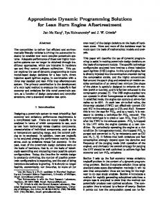
cost. Section V concludes the paper. II. P ROBLEM F ORMULATION A. System Description In this section we describe the model abstraction we adopted for this study. This model is primarily derived from the IEEE 802.15.4 specication as mentioned earlier. Consider N users sharing a common channel to send packets to a single server. Time is slotted and indexed by t = 0, 1, 2, · · · . Users alternate between on/active and off/inactive periods, and the duty cycle is dened as the fraction of time a user is on/active. An active period is M slots in length (M ≥ 1), and an inactive period is M ·(L−1) slots in length (L ≥ 1), resulting in a duty cycle of 1/L. For simplicity, L is assumed to be an integer. In words, during each cycle/period, the system is active for M slots (e.g., from t = 0 to t = M − 1 for the rst cycle) and then goes to sleep for (L − 1) · M slots. Then it becomes active again at the beginning of the LM -th slot and the same cycle repeats. The synchronization of users to ensure they adhere to the same active schedule is typically maintained via a beacon sent by the server right at the end of each cycle. That is, a user will wake up right before an active period, wait for the beacon, and resynchronize (e.g., to x clock drift, etc.). Since the beacon is typically very short compared to the slot or the cycle, we will ignore its duration. We assume that at the beginning of each active period, the server has the backlog and connectivity information (dened below) on each user in the system. This is a simplication. In reality, this information may be communicated via certain designated mini-slots at the beginning of each active period (between the beacon and the rst slot). The allocation decision is then made by the server and announced in a second beacon. For simplicity, the duration of these minislots are not considered in our formulation, although this does not affect the applicability of our analysis or results. The above system is shown in Figure 1. During each active time slot a user may or may not be connected to the server. If the user is not connected to the server, then it cannot transmit. Let qi,t denote the connectivity of user i at time t. If user i is connected to the server at time t then qi,t = 1, otherwise it is zero. If user i is connected to the server and the slot is allocated to it, then it transmits a packet successfully with probability pi . These success probabilities are assumed known by the server. At the beginning of every active period t, the server observes the queue-size of all the queues, denoted by bt , and their connectivity qt . The server uses this information to allocate the M slots among users and announces the allocation decision. This is achieved via the mini-slots and the second beacon as described above. The users subsequently follow the allocation decision and transmit in their designated slots (if they are assigned any). The whole system then goes to sleep for (L − 1)M time slots. At time t = LM the cycle repeats (ignoring the time spent by beacons and mini-slots).
Mini!slots User information advertised Decision announced in 2nd beacon Used for following slots Tin 1st beacon
Tac
(n+1)!th frame
n!th frame
Fig. 1.
The low duty cycle dynamics
We assume that a packet in queue i incurs a holding cost of ci for every slot it remains in the queue. The cost is collected at the end of each time slot. For instance the cost of time slot t (time interval [t, t + 1]) of queue i is equal to ci bi,[t+1]− where bi,[t+1]− is the backlog of queue i right before time t + 1. The objective is to nd an allocation policy π that minimizes the following cost function: JTπ C
= E π [C|F0 ], T −1 N ! ! βt ci bi,[t+1]− , = t=0
(1)
i=1
where F0 summarizes all the information available at time t = 0, and β < 1 is the discount factor. Consider a greedy policy π ∗ dened as follows. The server allocates an active slot at time t to user i such that i = argmaxj:qj,t =1,bj,t >0 cj pj , i.e., among the non-empty and connected queues the policy selects the queue with the largest index ci pi , which may be viewed as the immediate expected cost reduction (In case of multiple slot assignment we assume that the connectivity and backlog for each slot are known. More will be discussed in Section III-B). This greedy policy is in general not optimal, shown by the following example. Example 1: Suppose M = 1. Consider two users with c1 = 10 and c2 = 5. Assume that there are no arrivals; queue 1 is always connected; queue 2 is connected with probability q2 independently in each slot. Suppose there is one packet in each queue to be transmitted and the success probability is one for both queues. Obviously queue 1 has a higher index than queue 2. Suppose both queues are connected at time t = 0. Consider an innite time horizon, two policies π and π # are dened as follows. (1) π is the greedy policy, i.e. it assigns the slot at time t = 0 to queue 1 and then allocates the slot to queue 2 until the packet is successfully transmitted. (2) π # assigns the slot at t = 0 to queue 2 and assigns the next active slot to queue 1. Since queue 1 is always connected and the success probability is one both queues will be empty after time t = L. The expected cost from the above policies can be calcu-
lated as follows, denoting by ri = ci + βci + · · · + β L−1 ci : E π [C|F0 ] = "
E π [C|F0 ] =
∞ !
β kL (1 − q2 )k r2 =
k=0 L−1 !
1−
r2 L β (1
− q2 )
β t c1 = r1 .
t=0
"
β, L and q2 can be easily chosen so that E π [C|F0 ] < E π [C|F0 ] (an example is β = 0.9, q2 = 0.3, L = 2). Therefore the greedy policy is not in general optimal. In the next section we provide sufcient conditions under which this greedy policy is optimal under different assumptions on the user connectivity processes. B. Summary of Notations and Assumptions We consider time evolution in discrete time steps indexed by t = 0, 1, · · · T − 1, with each increment representing a time slot length. Slot t refers to the time interval [t, t + 1). In subsequent discussions we will use terms slots, steps and stages interchangeably. A frame consists of an active interval followed by an inactive interval. The rst frame starts from t = 0 and ends at t = M L which is the M L-th time slot. The second frame starts at t = M L and so on. We will use subscripts to denote the time index and to denote a specic user/queue. For example bi,t denotes the buffer occupancy at the beginning of time slot t for the i-th queue. All boldface letters represent column vectors and all normal letters represent scalars/random variables. Whenever we need to distinguish two policies, we show the policy as a superscript. For example bπi,t means the backlog of queue i at time t under policy π. A list of important notations is as follows. M : The length of the active period in number of slots. L: the length of a cycle in multiples of M slots, i.e., a cycle has a length of LM slots. Equivalently, L is the inverse of the duty cycle. bt = [b1,t , b2,t , · · · bN,t ]# : The column vector of all queue occupancies at time t. bi+ t = bt +ei , where ei is the N dimensional vector with all the values being zero except a one in the i-th position. at = [a1,t , a2,t , · · · aN,t ]# : The number of packet arrivals during time slot t. qt : The channel connectivity during the t-th time slot. pi : The transmission success probability of queue i. Ft : The σ-eld of the information available up to time t. Below we summarize important assumptions underlying our network model.
1) We assume that each user has an innite buffer. Without this assumption we need to introduce penalty for packet dropping/blocking. This is an important extension to the work presented here but is out of the scope of this paper. 2) We assume that the slot allocation for active period starting at time t cannot be used to transmit the possible packet arrival during the tth slot, i.e., within [t, t + 1). This is because the exact arrival time of this packet is random, and unless it arrives right before t it cannot be transmitted during that slot. 3) We assume that the channel state does not change during an active time slot. 4) We assume that the acknowledgments are immediate (i.e. we nd out whether a transmission is successful or not at the beginning of the next slot.) III. S UFFICIENT C ONDITIONS FOR THE O PTIMALITY OF THE G REEDY P OLICY In this section we study the optimality of the greedy policy discussed earlier. To make the discussion simpler we start by considering the case where an active period consists of a single slot M = 1. We then generalize the results to the case where M > 1. We also assume that T is an integer multiple of M L, the length of a cycle. This assumption allows us to keep the results in a simple form, but it can be easily relaxed. A. Single Slot Active Period Let M = 1, i.e. there is only one slot to allocate during an active period. Note that in this case active time slots are those at t = 0, L, 2L, · · · , TL − 1. The following lemma holds true regardless of any assumptions on the connectivity of the queues. Lemma 1: Let π be the optimal policy for state b0 and let π # be the optimal policy for state bi+ 0 . Then we have, "
π E π [C|F0 , bi+ 0 ] − E [C|F0 , b0 ] ≤
ci (1 − β T ) 1−β
(2)
Proof: π is an optimal policy given the initial state b0 . Let π ˆ be a policy dened for the initial state bi+ 0 , that schedules the exact same queues as policy π does for b0 . We ˆ now compare applying π starting with b0 with applying π starting with bi+ 0 . Since they both schedule the same queue every slot, in the worst case, the latter would end up having one more packet in queue i throughout the entire horizon. Therefore, π E πˆ [C|F0 , bi+ 0 ] − E [C|F0 , b0 ] T −1 ! ci (1 − β T ) ≤ a.s. β t · ci = 1−β t=0
(3)
On the other hand policy π ˆ is not necessarily the optimal policy for the initial state bi+ 0 . Therefore, "
i+ π E πˆ [C|F0 , bi+ 0 ] ≥ E [C|F0 , b0 ]
a.s.
(4)
Combining the two inequalities (3) and (4) proves the lemma. Below we consider two models for the channel connec" tivity and derive lower bounds on the value E π [C|bi+ 0 ]− E π [C|b0 ]. 1) No Information on Connectivity: In this part we assume the following about the channel connectivity. No-info - At the beginning of each active slot, the server is informed about the connectivity for that slot, but the server does not know the statistics of the connectivity process, e.g., it does not know how the connectivity changes from one time slot to the other. Lemma 2: Let π be the optimal policy for the initial state b0 and let π # be the optimal policy for state bi+ 0 . If there is no information about the channel connectivity process, then we have "
π E π [C|F0 , bi+ 0 ] − E [C|F0 , b0 ] T
≥
ri (1 − pi )(1 − (β L (1 − pi )) L ) , 1 − β L (1 − pi )
(5)
where ri = ci + βci + · · · β L−1 ci .
Proof: π # is an optimal policy given the initial state . Let π ˆ be a policy dened for the initial state b0 , that bi+ 0 schedules the exact same queues as policy π # does for initial ˆ starting with b0 state bi+ 0 . We now compare applying π with applying π # starting with bi+ . 0 Dene stopping time τ1 to be the rst time that queue " i has a successful transmission under policy π starting i+ with b0 , and that queue i does not have a successful transmission under policy π ˆ starting with b0 . Note that since both policies allocate to the same queue in each slot, this " is also the rst time when queue i is non-empty under π i+ and b0 , and is empty under π ˆ and b0 . Then we have τ1 ! " π ˆ E π [C|F0 , bi+ ] − E [C|F , b ] ≥ E[ β t−1 ci ] (6) 0 0 0 t=0
Dene stopping time τ2 to be the rst time queue i has a successful transmission under a policy that always transmit from queue i and given that queue i is always connected (let τ2 = T if this event does not occur before T −1). It can be seen that τ2 ≤ τ1 almost surely. Note that τ2 can occur in one of the time slots 0, L, 2L, · · · and the probability that it happens in time slot kL < T, k ≥ 0 is equal to pi (1 − pi )k . Therefore we have: "
π ˆ E π [C|F0 , bi+ 0 ] − E [C|F0 , b0 ] τ 2 ! ≥ E[ β t−1 ci ] t=0
=
T L −1
!
k=0
=
β kL (1 − pi )k+1 ri T
ri (1 − pi )(1 − (β L (1 − pi )) L ) 1 − β L (1 − pi )
(7)
On the other hand, policy π ˆ is not necessarily optimal for initial state b0 . Therefore, E π [C|F0 , b0 ] ≤ E πˆ [C|F0 , b0 ]
a.s.
(8)
Combining the two inequalities (7) and (8) proves the lemma. Theorem 1: Suppose the initial backlog state is b0 and suppose queues i and j are connected and non-empty. Let π be the policy that allocates the slot to queue i and let π # be the policy that allocates the slot to queue j. If there is no information available on the statistics of channel connectivity (No-info), but only that they are both connected in the current slot, then we have "
E π [C|F0 , b0 ] ≤ E π [C|F0 , b0 ], if T
ri (1 − pi )(1 − (β L (1 − pi )) L −1 ) ) 1 − β L (1 − pi ) cj (1 − β T −L ) . (9) ≥ pj rj + β L pj 1−β pj cj (1−β T ) (Note that the right hand side is simply equal to , 1−β but we leave it in this form to make it easier to compare the two sides). pi ri + β L pi (
Proof: Let Si denote the event that the transmission from queue i at time t = 0 is successful and let Si# denote the complement of this event, i.e. the transmission is not successful. Then we have: π"
E [C|F0 , b0 ] − E [C|F0 , b0 ] π
"
= pi pj (E π [C|F0 , b0 , Si ] − E π [C|F0 , b0 , Sj ]) "
+pi (1 − pj )(E π [C|F0 , b0 , Si ] − E π [C|F0 , b0 , Sj# ]) "
+(1 − pi )pj (E π [C|F0 , b0 , Si# ] − E π [C|F0 , b0 , Sj ]) +(1 − pi )(1 − pj )(E π [C|F0 , b0 , Si# ] "
− E π [C|F0 , b0 , Sj# ]) .
Note that the last term in the above equality is zero. Rearranging the other terms we get "
E π [C|F0 , b0 ] − E π [C|F0 , b0 ] "
= pi (E π [C|F0 , b0 , Si ] − E π [C|F0 , b0 , Sj# ]) "
+pj (E π [C|F0 , b0 , Si# ] − E π [C|F0 , b0 , Sj ]) . "L−1 Let a = t=0 at and bL = b0 + a, then we have "
E π [C|F0 , b0 ] − E π [C|F0 b0 ] = −pi ri + pj rj π
"
+pj (E π [C|FL , bL ] + E π [C|FL , bL − ej ])}
≤ −pi ri + pj rj
T
ri (1 − pi )(1 − (β L (1 − pi )) L −1 ) ) 1 − β L (1 − pi ) cj (1 − β T −L ) }, +pj 1−β
+β L {−pi (
Corollary 1: Suppose the state at t = 0 is b0 and suppose queue i is connected and non-empty. If there is no information on the statistics of the channel connectivity process, then it is optimal to allocate the slot at t = 0 to queue i if (9) holds for all j $= i such that qj,0 = 1 and bj,0 > 0. 2) Independent Connectivity: In this part we assume the following about the channel connectivity. Indep - At each active time slot, user i is connected to the server with probability qi independent of all past history. The quantities qi is known to the server. In addition, at the beginning of each active time slot the server knows whether a queue is connected for that slot. This assumption is valid if for example the length of the inactive period is very large in comparison with the channel variations, so that the channel states during successive active periods appear independent. Lemma 3: Let π be the optimal policy for state b0 and let π # be the optimal policy for state bi+ 0 . If the channel changes state independently at the beginning of each active slot, then we have "
π E π [C|F0 , bi+ 0 ] − E [C|F0 , b0 ]
≥
T
ri (1 − pi qi )(1 − (β L (1 − pi qi )) L ) , 1 − β L (1 − pi qi )
(10)
where ri = ci + βci + · · · β L−1 ci .
Proof: Dene policy π ˆ and stopping time τ1 the same way as in lemma 2. Dene stopping time τ2 to be the rst time queue i has a successful transmission under a policy that always transmit from queue i (let τ2 = T if this event does not occur before T − 1). It can be seen that τ2 ≤ τ1 almost surely. Note that τ2 can occur in one of the time slots 0, L, 2L, · · · and the probability that it happens in time slot kL < T, k ≥ 0 is equal to pi qi (1 − pi qi )k . Therefore we have: "
π ˆ E π [C|F0 , bi+ 0 ] − E [C|F0 , b0 ] τ 2 ! ≥ E[ β t−1 ci ] t=0
=
T L −1
!
k=0 π"
+β {pi (E [C|FL , bL − ei ] − E [C|FL , bL ]) L
where the inequality is a result of Lemmas 1 and 2 (note that T has been replaced by T −L since the initial condition starts from time L). It can be seen that if (9) holds then we " have E π [C|F0 , b0 ] ≤ E π [C|F0 , b0 ].
β kL (1 − pi qi )k+1 ri T
ri (1 − pi qi )(1 − (β L (1 − pi qi )) L ) (11) = 1 − β L (1 − pi qi ) On the other hand, policy π ˆ is not necessarily optimal for initial state b0 . Therefore, E π [C|F0 , b0 ] ≤ E πˆ [C|F0 , b0 ]
a.s.
(12)
Combining the two inequalities (11) and (12) proves the lemma.
Theorem 2: Suppose the initial state is b0 and suppose queues i and j are connected and non-empty. Let π be the policy that allocates the slot to queue i and let π # be the policy that allocates the slot to queue j. Using the channel model dened by Indep, we have "
E π [C|F0 , b0 ] ≤ E π [C|F0 , b0 ] , if the following inequality holds: T
ri (1 − pi qi )(1 − (β L (1 − pi qi )) L −1 ) ) 1 − β L (1 − pi qi ) cj (1 − β T −L ) ≥ pj rj + β L pj . (13) 1−β The proof of this theorem is similar to the proof of Theorem 1 and is therefore omitted. pi ri + β L pi (
Corollary 2: Suppose the state at t = 0 is b0 and suppose queue i is connected and non-empty. If the channel model is as Indep, then it is optimal to allocate the slot at t = 0 to queue i if (13) holds for all j $= i such that qj,0 = 1 and bj,0 > 0. Remark 1: Note that the sufcient condition in Theorem 2 (Equation (13)) is weaker than the one in Theorem 1 (Eqn (9)), i.e. it is satised more easily. Essentially the information on the connectivity process allows us to derive a tighter bound for the optimality of the greedy policy. Remark 2: As L increases the sufcient conditions (9) and (13) become weaker. Specically in the limit as L → ∞ it can be seen that it is optimal to serve queue i if pi ci ≥ pj cj for all j $= i which is essentially the greedy policy. Therefore in this case the sufcient conditions are tight and the greedy policy is optimal. Remark 3: Although all theorems in this section are based on the optimal allocation at time t = 0, it can be seen that all the results can be easily extended to the bandwidth allocation at time t by replacing T with T − t in all the sufcient conditions. This is due to the fact that T is essentially the ”time to go” in all these results and if we start at time t, then the time to go is T − t. B. Multiple Slot Active Period In this part we assume M > 1 and nd the sufcient conditions for the optimality of the greedy policy, using the same channel connectivity models dened in Section III-A. Note that in the case of M > 1, the allocation decision made by the server is delayed, in the sense that the server uses the backlog information at time t to make the allocation decision for time t, t + 1, · · · , t + M − 1. By the time the m-th slot (m > 1) is used (at time slot t + m − 1), the backlog of the queues may have changed. In order to avoid complications caused by this information delay we make the following assumption. Assumption 1: When M > 1 the server makes the allocation decision for each active time slot individually. At each active time slot the server knows the backlog and
connectivity of all the queues during that time slot before making the allocation decision. This assumption certainly holds in the case of down-link communication (from the server to the users). In the uplink, as long as the length of the active period is small compared to the arrival probability, this is a good approximation. In any case this assumption introduces a lower bound on the cost of the real system (with information delay). Note that Lemma 1 holds in the case of multiple slot active period as well. The proofs of the following results are very similar to the proofs in Section III-A. Therefore, we have omitted the proofs in this part. Lemma 4: Let π be the optimal policy for state b0 and let π # be the optimal policy for state bi+ 0 . If the channel state process is not known, then we have "
π E π [C|F0 , bi+ 0 ] − E [C|F0 , b0 ] T
≥ where # = ri,m
M −1 !
k=m−1
# (1 − (β M L (1 − pi )M ) M L ) ri,1 , 1 − β M L (1 − pi )M
β k (1 − pi )k−m+2 ci +
LM −1 ! k=M
β k (1 − pi )M ci .
Theorem 3: Let t be the m-th active slot of an active period and let t# = t − m + 1 (this is the rst slot of the active period). Suppose the state at t is bt and suppose queue i is connected and non-empty. If the channel model is as dened by No-info and there are M slots per active period, then it is optimal to allocate the slot at time t to queue i if the following inequality holds for all j $= i such that qj,t = 1 and bj,t > 0: T −t" +1
# # ri,1 (1 − (β M L (1 − pi )M ) M L −1 ) pi ri,m + β M L pi 1 − pi 1 − β M L (1 − pi )M " # pj rj,m cj (1 − β T −t −M L ) . (14) ≥ + β M L pj 1 − pj 1−β The following results are for the case of independent channel connectivity (Indep).
Lemma 5: Let π be the optimal policy for state b0 and let π # be the optimal policy for state bi+ 0 . If the channel changes state independently at the beginning of each active slot, then we have "
π E π [C|bi+ 0 ] − E [C|b0 ]
≥ where ## ri,m
T
## (1 − (β M L (1 − pi qi )M ) M L ) ri,1 1 − β M L (1 − pi qi )M ,
=
M −1 !
k=m−1
+
β k (1 − pi qi )k−m+2 ci
LM −1 ! k=M
β k (1 − pi qi )M ci .
4
## (ri,1 (1 − (β M L (1 − pi qi )M ) M L +β pi 1 − β M L (1 − pi qi )M ) " ## pj rj,m cj (1 − β T −t −M L ) L ≥ + β pj 1 − pj 1−β ML
−1
M=1 M=5 M = 10 M = 15
6
5
4
3
(15) T −t"
x 10
7
2
)
1
0
1
2
3
4
5
6
7
8
9
10
L (a) 5
(16)
Remark 4: All the results presented in this section hold for all values of T . Specically one can let T → ∞ to derive the sufcient conditions for the optimality of the greedy policy in the case of an innite horizon. IV. N UMERICAL A NALYSIS As shown earlier, the greedy policy is not necessarily optimal and in the previous section we found sufcient conditions for its optimality. In this section we will x this policy, regardless of whether it is optimal for the scenarios considered, and study the performance of this policy via a few numerical examples. In particular, we are interested in (1) how the performance of this policy (in terms of packet holding cost) varies as the duty cycle ( L1 ) changes while xing the active period M ; and (2) how the performance varies as M changes while xing L (i.e., xing the duty cycle but varying the frequency of cycling). Note that as L increases the duty cycle decreases and therefore we expect the total cost to increase. On the other hand large L means longer inactive intervals, which implies longer lifetime of the system. Therefore it is important to see how the performance degrades as the lifetime increases. The effect of M is more complicated. As M increases (for xed L) the system has longer cycles, i.e., switches between on and off periods less often. This in turn increases the system lifetime as turning devices on and off typically consumes nonnegligible energy especially for low power devices. But at the same time, longer cycles also increases the probability that an active slot coincides with empty queues which causes performance degradation. We assume that the channel states in different slots are independent, with a xed connectivity probability. The server does not need to know this probability (in fact the greedy policy does not require any information about how the state changes, it only needs to know the current state and the current backlog). While it is obvious that a very limited number of examples considered in this section are certainly not sufcient for a full characterization of the behavior of the system in general, they nevertheless provide some interesting insight on the properties of the greedy policy and the effect of parameters like M and L.
4.5
4
3.5 backlog of queue 1
## ri,m pi 1 − pi qi
8
cost
Theorem 4: Let t be the m-th active slot of an active period. Let t# = t − m + 1. Suppose the state at t is bt and suppose queue i is connected and non-empty. If the channel model is as dened by Indep and there are M slots per active period, then it is optimal to allocate the slot at t = 0 to queue i if the following inequality holds for all j $= i such that qj,t = 1 and bj,t > 0:
3
2.5
2
1.5
1
0.5
0
0
100
200
300
400
500 time (b)
600
700
800
900
1000
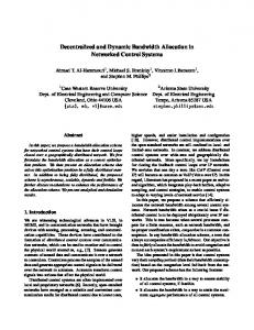
Fig. 2. First scenario: a) Cost Variation as a function of L and M , rst scenario, b) rst queue’s backlog as a function of time
For the rst example consider the following scenario. There are two queues. Arrivals are Bernoulli, i.e. at each time slot there is an arrival to queue i with probability ui and there are no arrivals with probability 1 − ui . Other parameters are as follows: β = 0.999, T = 1000, c1 = 15, c2 = 5, u1 = 0.05; u2 = 0.05; p1 = 0.9; p2 = 0.6; q1 = 0.7; q2 = 0.9. Figure 2-a illustrates the total cost as a function of L. Different curves correspond to different values of M . The curve is an average over 200 simulations. Note that in this case as M increases the curve shifts up. This clearly shows that small M , i.e., shorter cycles or more frequent on/off switching performs better. The signicance of this observation is made clear in comparison with the second example below. Figure 2-b shows the backlog variation of an example sample path for L = 5 and M = 5. For the second example consider the same scenario above with the following parameters: β = 0.999, T = 1000, c1 = 15, c2 = 5, u1 = 0.05; u2 = 0.05; p1 = 0.7; p2 = 0.6; q1 = 0.5; q2 = 0.9. Figure 3-a illustrates the total cost as a function of L. Different curves correspond to different values of M . The curve is an average over 200 simulations. Note that in this case increasing M has a much smaller effect on the cost performance compared to the rst example. In this example, the frequency of cycling made little difference in terms of costs for the same duty cycle. Figure
4
16
x 10
(one step gain). We provided sufcient conditions for this greedy policy to be optimal. We then studied the effect of changing the duty cycle and the number of active slots per frame on the performance of the greedy policy. The performance degrades as the duty cycle decreases. When the system is near the boundary (the queues are empty most of the time) increasing the number of active slots per frame (M ) degrades the performance. On the other hand decreasing the duty cycle and increasing M increases the lifetime of the system. Comprehensive modeling of this tradeoff is part of our future study.
M=1 M = 10 M = 15
14
12
cost
10
8
6
4
2
0
1
2
3
4
5
6
7
8
9
10
L (a) 6
5
backlog of queue 1
4
3
2
1
0
0
100
200
300
400
500 time (b)
600
700
800
900
1000
Fig. 3. Second scenario: a) Cost Variation as a function of L and M , rst scenario, b) rst queue’s backlog as a function of time
2-b shows the backlog variation of an example sample path for L = 5 and M = 5. In comparison with the rst example, we note that the only difference in system parameters is that in the second case queue 1 has a smaller success probability and a smaller connectivity probability. This translates into more packets queued up in the system than in the rst example. As a result, we see that the queues do not become empty as often as the previous scenario. Consequently, multiple slot allocation at a time (M > 1) is well utilized in that there is a highly probability that these slots are used and the queues are less likely to become empty. By comparison, the parameters of the rst example result in empty queues more often and therefore it is less efcient to allocate multiple slots at a time (it is more likely that some of the slots are not utilized due to empty queues). In this case, it is better to have shorter active periods but cycle the system more frequently; this is the difference observed in Figure 2 for different values of M . V. C ONCLUSION In this paper we analyzed the optimality of an index/greedy policy for allocating time slots in a low duty cycled system. Each user is associated with a connectivity probability and a transmission success probability. The greedy policy allocates the channel to the non-empty connected queue with the largest immediate expected cost
R EFERENCES [1] J. S. Baras, A. J. Dorsey, and A. M. Makowski, “Two competing queues with linear costs and geometric service requirements: The µc rule is often optimal,” Adv. Appl. Prob., vol. 17, pp. 186–209, 1985. [2] C. Buyukkoc, P. Varaiya, and J. Warland, “The cµ-rule revisited,” Advances in Applied Probability, vol. 17, pp. 237–238, 1985. [3] J. G. Shanthikumar and D. D. Yao, “Multi class queueing systems: Polymatroid structure and optimal scheduling control,” Oper. Res., vol. 40, pp. 293 – 299, 1992. [4] J. Edmonds, “Submodular functions, matroids and certain polyhedra,” In Proc. of the Calgary International Conference on Combinatorial Structures and Their Applications, Gordon and Breach, New York, pp. 69–87, 1970. [5] D. Bertsimas and J. Nino-Mora, “Conversion laws, extended polymatroids and multi-armed bandit problems,” Mathematics of Operations Research, vol. 21, pp. 257–306, 1996. [6] T. C. Green and S. Stidham Jr., “Sample path conservation laws, with applications to scheduling queues and uid systems,” Queueing Systems, vol. 36, pp. 175–199, 2000. [7] L. Tassiulas and A. Ephremides, “Dynamic server allocation to parallel queues with randomly varying connectivity,” IEEE Transactions on Information Theory, vol. 39, no. 2, pp. 466–478, March 1993. [8] L. Tassiulas, “Scheduling and performance limits of networks with constantly changing topology,” IEEE Transactions on Information Theory, vol. 43, no. 3, pp. 1067–73, May 1997. [9] N. Bambos and G. Michailidis, “On the stationary dynamics of parallel queues with random server connectivities,” Proc. 43th Conference on Decision and Control (CDC), pp. 3638–43, 1995, New Orleans, LA. [10] C. Lott and D. Teneketzis, “On the optimality of an index rule in multi-channel allocation for single-hop mobile networks with multiple service classes,” Probability in the Engineering and Informational Sciences, vol. 14, no. 3, pp. 259–297, July 2000. [11] M. J. Neely, E. Modiano, and C. E. Rohrs, “Power allocation and routing in a multibeam satellite with time-varying channels,” IEEE Proceedings of INFOCOM, 2002. [12] M. J. Neely, E. Modiano, and C. E. Rohrs, “Dynamic power allocation and routing for time-varying wireless networks,” IEEE/ACM Tansactions on Networking, Vol. 11, N0. 1, pp. 138–152, 2003. [13] B. Hajek, “Optimal control of two interacting service stations,” IEEE Trans. Auto. Control. AC-29, pp. 491–499, 1984. [14] J. C. Gittins, “Bandit processes and dynamic allocation indices,” J. Royal Statistical Society Series, vol. B14, pp. 148–167, 1972. [15] P. Whittle, “Multi-armed bandits and the gittins index,” Journal of the Royal Statistical Society, vol. 42, no. 2, pp. 143–149, 1980. [16] P. Whittle, “Restless bandits: Activity allocation in a changing world,” A Celebration of Applied Probability, ed. J. Gani, Journal of applied probability, vol. 25A, pp. 287–298, 1988. [17] R. Weber and G. Weiss, “On an index policy for restless bandits,” Journal of Applied Probability, vol. 27, pp. 637–648, 1990. [18] J. Nino-Mora, “Restless bandits, patial conservation laws, and indexability,” Advances in Applied Probability, Vol. 33, no. 1, pp. 76–98, 2001. [19] C. H. Papadimitriou and J. N. Tsitsiklis, “The complexity of optimal queueing network control,” Mathematics of Operations Research, Vol. 24, No. 2, pp. 293–305, May 1999.