Dynamic Bayesian Networks for Vehicle Classification in Video - VISLab

IEEE TRANSACTIONS ON INDUSTRIAL INFORMATICS

1

Dynamic Bayesian Networks for Vehicle Classification in Video Mehran Kafai, Student Member, IEEE, and Bir Bhanu, Fellow, IEEE

Abstract— Vehicle classification has evolved into a significant subject of study due to its importance in autonomous navigation, traffic analysis, surveillance and security systems, and transportation management. While numerous approaches have been introduced for this purpose, no specific study has been conducted to provide a robust and complete video-based vehicle classification system based on the rear-side view where the camera’s field of view is directly behind the vehicle. In this paper we present a stochastic multi-class vehicle classification system which classifies a vehicle (given its direct rear-side view) into one of four classes Sedan, Pickup truck, SUV/Minivan, and unknown. A feature set of tail light and vehicle dimensions is extracted which feeds a feature selection algorithm to define a low-dimensional feature vector. The feature vector is then processed by a Hybrid Dynamic Bayesian Network (HDBN) to classify each vehicle. Results are shown on a database of 169 videos for four classes. Index Terms— Classification, Hybrid Dynamic Bayesian Network.

I. I NTRODUCTION VER the past few years vehicle classification has been widely studied as part of the broader vehicle recognition research area. A vehicle classification system is essential for effective transportation systems (e.g., traffic management and toll systems), parking optimization, law enforcement, autonomous navigation, etc. A common approach utilizes vision-based methods and employs external physical features to detect and classify a vehicle in still images and video streams. A human being may be capable of identifying the class of a vehicle with a quick glance at the digital data (image, video) but accomplishing that with a computer is not as straight forward. Several problems such as occlusion, tracking a moving object, shadows, rotation, lack of color invariance, and many more must be carefully considered in order to design an effective and robust automatic vehicle classification system which can work in real-world conditions. Feature based methods are commonly used for object classification. As an example, Scale Invariant Feature Transform (SIFT) represents a well-studied feature based method. Using SIFT an image is represented by a set of relatively invariant local features. SIFT provides pose invariance by aligning features to the local dominant orientation and centering features at scale space maxima. It also provides appearance change resilience and local deformation resilience. To the contrary,

O

Manuscript received April 30, 2011; revised August 19, 2011 and September 19, 2011. Accepted for publication October 9, 2011. This work was supported in part by NSF grant number 0905671. The content of the information do not reflect the position or policy of the US Government. Copyright 2012 IEEE. Personal use of this material is permitted. However, permission to use this material for any other purposes must be obtained from the IEEE by sending a request to [email protected]. Mehran Kafai is with the Center for Research in Intelligent Systems, Computer Science Department, University of California at Riverside, Riverside, CA 92521 (email: [email protected]). Bir Bhanu is with the Center for Research in Intelligent Systems, University of California at Riverside, Riverside, CA 92521 (email: [email protected]).

reliable feature extraction is limited when dealing with low resolution images in the real-world conditions. Much research has been conducted for object classification, but vehicle classification has shown to have its own specific problems which motivates research in this area. In this paper, we propose a Hybrid Dynamic Bayesian Network as part of a multi-class vehicle classification system which classifies a vehicle (given its direct rear-side view) into one of four classes: Sedan, Pickup truck, SUV/Minivan, and unknown. High resolution and close up images of the logo, license plate, and rear view are not required due to the use of simple low-level features (e.g., height, width, and angle) which are also computationally inexpensive. In the rest of this paper, Section II describes the related work and contributions of this work. Section III discusses the technical approach and system framework steps. Section IV explains the data collection process and shows the experimental results. Finally, Section V concludes the paper. II. R ELATED W ORK AND O UR C ONTRIBUTIONS A. Related Work Not much has been done on vehicle classification from the rear view. For the side view, appearance based methods especially edge-based methods have been widely used for vehicle classification. These approaches utilize various methods such as weighted edge matching [1], Gabor features [2], edge models [3], shape based classifiers, part based modeling, and edge point groups [4]. Model-based approaches that use additional prior shape information have also been investigated in 2D [5] and more recently in 3D [6], [7]. Shan et al. [1] presented an edge-based method for vehicle matching for images from nonoverlapping cameras. This feature-based method computed the probability of two vehicles from two cameras being similar. The authors define the vehicle matching problem as a 2-class classification problem, thereafter apply a weak classification algorithm to obtain labeled samples for each class. The main classifier is trained by a unsupervised learning algorithm built on Gibbs sampling and Fisher’s linear discriminant using the labeled samples. A key limitation of this algorithm is that it can only perform on images that contain similar vehicle pose and size across multiple cameras. Wu et al. [3] use a parameterized model to describe vehicle features, thenceforth embrace a multi-layer perceptron network for classification. The authors state that their method falls short when performing on noisy and low quality images and that the range in which the vehicle appears is small. Wu et al. [8] propose a PCA based classifier where a sub-space is inferred for each class using PCA. As a new query sample appears, it is projected onto all class sub-spaces, and is classified based on which projection results in smaller


residue or truncation errors. This method is used for multiclass vehicle classification for static road images. Experiments show it has better performance compared to linear Support Vector Machine (SVM) and Fisher Linear Discriminant (FLD). Vehicle make and model recognition from the frontal view is investigated in [9] and more recently in [10]. Psyllos et al. [10] use close up frontal view images and a neural network classifier to recognize the logo, manufacturer, and model of a vehicle. The logo is initially segmented and then used to recognize the manufacturer of the vehicle. The authors report 85% correct recognition rate for manufacturer classification and only 54% for model recognition. Such an approach entirely depends on the logo, therefore, it might fail if used for the rear view as the logo may not always be present. For the rear view, Dlagnekov et al. [11] develop a vehicle make and model recognition system for video surveillance using a database of partial license plate and vehicle visual description data, and they report a recognition accuracy of 89.5%. Visual features are extracted using two featurebased methods (SIFT and shape context matching) and one appearance-based method (Eigencars). The drawbacks of the proposed system are that it is relatively slow, and only the license plate recognition stage is done in real-time. A summary of related work is shown in Table I.

2

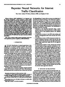
(a) Vehicle boundary

(b) Resulting time series using ra- (c) Resulting time series using local dius distance neighborhood curvature Fig. 1.

Converting vehicle boundary shape into time series

reasons. First, most of the research in this area has focused on the side view ([2], [1], [3]) whereas the frontal view and rear view have been less investigated. Secondly, not all states require a front license plate (19 states in the USA require only the rear license plate). We introduce a Hybrid Dynamic Bayesian Network (HDBN) classifier with multiple time slices corresponding to multiple video frames.

TABLE I R ELATED W ORK S UMMARY

Author Psyllos et al. [10] Conos et al. [9] Chen et al. [12] Zhang et al. [13] Shan et al. [1] Wu et al. [3] This Paper

Principles & Methodology frontal view, neural network classification, Phase congruency calculation, SIFT fingerprinting frontal view, kNN classifier, SIFT descriptors, frontal view images side view, multi-class SVM classifier, color histograms side view, shape features, wavelet fractal signatures, fuzzy k-means side view, edge-based, binary classification, Fishers Linear Discriminants, Gibbs sampling, unsupervised learning side view, neural network classification, parametric model rear view, Hybrid Dynamic Bayesian Network

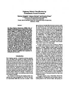
For the side view we have conducted a study for vehicle recognition using pseudo time series. After some preprocessing (moving vehicle detection, shadow removal) and automatically tracing the boundary pixels, the vehicle 2D blob shape is converted to a pseudo time series using either radius distance scanning or local neighborhood curvature. Figures 1(b) and 1(c) demonstrate the time series representing the sample vehicle boundary in Figure 1(a). Pseudo time series works well for side view vehicle classification (Section IV-A) but will not perform as well if used for frontal view or rear view due to boundary shape similarity. B. Contributions of this Paper Unlike the previous work as shown in Table I the contributions of this paper are: (a) We propose a probabilistic classification framework which determines the class of a vehicle given its direct rear view (Figure 2). We choose the direct rear view for two main

Fig. 2.

Sample images of the direct rear view of a moving vehicle

(b) We eliminate the need for high resolution and close up images of the logo, license plate, and rear view by using simple low-level features (e.g., height, width, and angle) which are also computationally inexpensive, thus, the proposed method is capable of running in real-time. (c) The results are shown on a database of 169 real videos consisting of Sedan, Pickup truck, SUV/minivan, and also a class for unknown vehicles. We adapt, modify, and integrate computational techniques to solve a new problem that has not been addressed or solved by anyone. Vehicle classification has been investigated by many people. The novelty of our work comes from using the HDBN classifier for rear view vehicle classification in video. Our approach is a solution to important practical applications used in law enforcement, parking security, etc. For example when a vehicle is parked in a parking lot the rear view is usually visible and the frontal view and side view images cannot be captured. In this case, rear view classification is essential for parking lot security and management. The key aspects of our paper are: • A novel structure for the HDBN is proposed, specifically designed to solve a practical problem. The HDBN classifier has never before been used in the context of proposed video application. Rear-side view classification has not been studied in video.


•

•

The HDBN is defined and structured in a way that adding more rear view features is easy, missing features that were not extracted correctly in one or more frames of a video are inferred in the HDBN and, therefore, classification does not completely fail. A complete system including feature extraction, feature selection, and classification is introduced with significant experimental results.

3

(a) original image

(b) moving object mask

(c) initial bounding box

(d) readjusted bounding box

III. T ECHNICAL A PPROACH The complete proposed system pipeline is shown in Figure 3. All components are explained in the following sections.

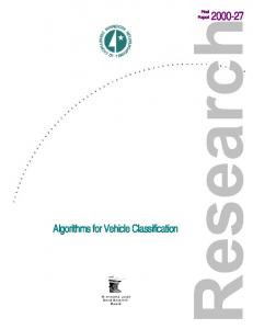
Fig. 4.

Fig. 3.

System Framework

A. Feature Extraction Three main types of features are extracted from the images; tail lights, license plate, and rear dimensions. The tail light features include separately for each tail light the width, distance from the license plate, and angle between tail light and license plate. The license plate location and size is used as a reference to enable comparison and help normalize tail light properties and vehicle size values. The feature extraction component consists of three subcomponents: vehicle detection, license plate extraction, and tail light extraction. 1) Vehicle Detection: Object detection is an active research topic in transportation systems([14], [15], [16], [17]). In this paper a Gaussian mixture model approach is used for moving object detection. The Gaussian distributions are used to determine if a pixel is more likely to belong to the background model or not. An AND approach is used which determines a pixel as background only if it falls within three standard deviations for all the components in all three R, G, and B color channels [18]. We validate the detected moving object by using a simple frame differencing approach and cross checking the masks from both methods. The resulting mask may include some shadow and erroneous pixels. The shadow is removed by finding the vertical axis of symmetry using an accelerated version of Loy’s symmetry [19] and readjusting the bounding box containing the mask with respect to the axis of symmetry. This is done by measuring the distance between each point on both vertical sides of the bounding box and the axis symmetry and moving the vertical side that is farther away closer to the axis of symmetry such that each side has the same distance from it. Figure 4 shows results from multiple steps of this approach. The aforementioned shadow removal method fails if the shadow is behind the vehicle. In such cases the shadow is removed using the approach introduced by Nadimi et al. [20] which does not rely on the common geometrical assumptions such as camera location, object geometry, and ground surface geometry. Given the vehicle rear mask, the height and width of the bounding box, and area of the mask are measured. 2) License Plate Extraction: We use the license plate corner coordinates as input to our algorithm. There are number of algorithms for license plate extraction ([21],[22]). Anagnostopoulo et al. [22] propose using Sliding Concentric Window

Shadow removal and obtaining the bounding box

segmentation, masking, and Sauvola binarization to identify the license plate location. They report a 96.5% success rate on a database of 1334 images. In this paper we have focused on novel aspects of HDBN classifier and the integrated system. This allows us to quantify the results at the system level independent of the particular algorithm used for license plate extraction. We have described a license detection approach in Section III-A.2.a. The classification results are obtained by manual license plate detection. However, the proposed or any other license detection algorithm can be easily integrated into our system. a) Automatic License Plate Extraction: The license plate is extracted using two separate methods and then the ”best” result is chosen. The first method is proposed by Abolghasemi et al. in [23] where a matched filtering approach is applied to extract candidate plate-like regions. The contrast of plate-like regions is enhanced using vertical edge density, and detection is performed using colored texture in the plate. In addition to the method from [23] we apply a blob detection and filtering method to improve license plate detection. This additional method consists of the followings steps: 1) Detect edges 2) Generate binary image with selectable blobs. Image is processed to accent the more apparent detected edges and to fill and smooth the image where appropriate. 3) Determine the blob that most likely corresponds to the license plate. In a cascading form, filter the blobs using the following attributes: blobs with a side length comparable to a license plate, blobs that are horizontally aligned, blob size relative to a license plate, squareness of blob, blobs that are far to linear in shape, closest ideal area, and closest total distant to the centroid from multiple points. The result from the method of vertical edge detection and match filtering is compared with the result from the method of blob detection and match filtering. Both methods are given a score on which solution is most likely the actual license plate. The scoring systems awards points for the following attributes: accurate license plate to bounding box ratios, the centering of the license plate returned across the axis of symmetry, how equal the centering on the axis of symmetry is, prediction of each side in comparison to the centroid, the average color of the license plate, and


the squareness presented by both solutions. The solution with the highest score value is then selected as the most accurate prediction of the license plate location. Figure 5 shows some results of the license plate extraction component. The overall

Fig. 5.

License plate extraction

license plate extraction rate is 98.2% on a dataset of 845 images. The extracted license plate height and width measurements for 93.5% of the dataset have ±15% error compared to the actual license plate dimensions, and 4.7% have between ±15% and ±30% error. 3) Tail Light Extraction: For tail light detection the regions of the image where red color pixels are dominant are located. We compute the redness of each image pixel by fusing two methods. In the first approach [24] the image is converted to HSV color space and then pixels are classified into three main color groups red, green, and blue. The second method proposed by Gao et al. [25] defines the red level of each i in RGB color space. A bounding box pixel as ri = G2R i +Bi surrounding each tail light is generated by combining results from both methods and checking if the regions with high redness can be a tail light (e.g., are symmetric, are close to the edges of the vehicle). Figure 6 presents results of the two methods and the combined result as two bounding boxes. Both

Fig. 6.

Tail light detection

these methods fail if the vehicle body color is red itself. To overcome this, the vehicle color is estimated using a HSV color space histogram analysis approach which determines if the vehicle is red or not. If a red vehicle is detected, the tail light detection component is enhanced by adding an extra level of post-processing which includes Otsu’s thresholding [26], color segmentation, removing large and small regions, and symmetry analysis. After the tail lights are detected, the width, centroid, and distance and angle with the license plate are separately computed for both left and right tail lights. Tail-light detection is challenging for red vehicles. Our approach performs well considering the different components involved (symmetry analysis, size filtering, thresholding, ...) . However, for more accurate tail light extraction Otsu’s method may not be sufficient. For our future work we plan to consider more sophisticated methods such as using physical models [20] to distinguish the lights from the body based on the characteristics of the material of a vehicle. 4) Feature Set: As the result of the feature extraction component the following 11 features are extracted from each image frame (all distances are normalized with respect to the license plate width):

4

1) perpendicular distance from license plate centroid to a line connecting two tail light centroids 2) right tail light width 3) left tail light width 4) right tail light-license plate angle 5) left tail light-license plate angle 6) right tail light-license plate distance 7) left tail light-license plate distance 8) bounding box width 9) bounding box height 10) license plate distance to bounding box bottom side 11) vehicle mask area A vehicle may have a symmetric structure but we chose to have separate features for the left side and right side so that the classifier does not completely fail if during feature extraction a feature (e.g., tail light) on one side is not extracted accurately. Also, the tail light-license plate angles may differ for the left and right side because the license plate may not be located in the center exactly. B. Feature Selection Given a set of features Y , feature selection determines a subset X which optimizes an evaluation criterion J. Feature selection is performed for various reasons including improving classification accuracy, shortening computational time, reducing measurements costs, and relieving the curse of dimensionality. We chose to use Sequential Floating Forward Selection (SFFS), a deterministic statistical pattern recognition (SPR) feature selection method which returns a single suboptimal solution. SFFS starts from an empty set and adds the most significant features (e.g., features that increase accuracy the most). It provides a kind of back tracking by removing the least significant feature during the third step, conditional exclusion. A stopping condition is required to halt the SFFS algorithm, therefore, we limit the number of feature selection iterative steps to 2n−1 (n is the number of features) and also define a correct classification rate (CCR) threshold of b% where b is greater than the CCR of the case when all features are used. In other words, the algorithm stops when either the CCR is greater than b%, or 2n−1 iterations are completed. Below the pseudocode for SFFS is shown (k is the number of features already selected). 1) Initialization: k = 0; X0 = {∅} 2) Inclusion: add the most significant feature xk+1 = arg maxx∈(Y −Xk ) [J(Xk + x)] Xk+1 = Xk + xk+1 ; repeat step 2 if k < 2 3) Conditional Exclusion: find the least significant feature and remove (if not last added) xr = arg maxx∈Xk [J(Xk − x)] if xr = xk+1 then k = k + 1; Go to step 1 else Xk0 = Xk+1 − xr 4) Continuation of Conditional Exclusion xs = arg maxx∈Xk0 [J(Xk0 − x)] if J(Xk0 − xs ) ≤ J(Xk−1 ) then Xk = Xk0 ; Go to step 2 0 else Xk−1 = Xk0 − xs ; k = k − 1 5) Stopping Condition Check if halt condition = true then STOP else Go to step 4 Figure 7 presents the correct classification rate plot with feature selection steps as the x-axis and correct classification rate as the y-axis. The plot peaks at x = 5 and the algorithm


5

returns features 1, 4, 6, 10, and 11 as the suboptimal solution.

(a) K2 generated structure

Fig. 7.

Feature selection subset CCR plot

C. Classification 1) Known or Unknown class: The classification component consists of a two stage approach. Initially the vehicle feature vector is classified as known or unknown. To do such, we estimate the Gaussian distribution parameters of the distance to the nearest neighbor for all vehicles in the training dataset. To determine if a vehicle test case is known or unknown first the distance to its nearest neighbor is computed. Then following the empirical rule if the distance does not lie within 4 standard deviations of the mean (µ ± 4σ) it is classified as unknown. If the vehicle is classified as known it is a candidate for the second stage of classification. 2) DBNs for Classification: We propose to use Dynamic Bayesian Networks (DBNs) for vehicle classification in video. Bayesian networks offer a very effective way to represent and factor joint probability distributions in a graphical manner which makes them suitable for classification purposes. A Bayesian network is defined as a directed acyclic graph G = (V, E) where the nodes (vertices) represent random variables from the domain of interest and the arcs (edges) symbolize the direct dependencies between the random variables. For a Bayesian network with n nodes X1 , X2 , . . . , Xn the full joint distribution is defined as: p(x1 , x2 , . . . , xn ) = p(x1 ) × p(x2 |x1 ) × . . . × p(xn |x1 , x2 , . . . , xn−1 ) n Y = p(xi |x1 , . . . , xi−1 )

(1)

i=1

but a node in a Bayesian network is only conditional on its parent’s values so p(x1 , x2 , . . . , xn ) =

n Y

p(xi |parents(Xi ))

(2)

i=1

where p(x1 , x2 , . . . , xn ) is an abbreviation for p(X1 = x1 ∧ . . . ∧ Xn = xn ). In other words, a Bayesian network models a probability distribution if each variable is conditionally independent of all its non-descendants in the graph given the value of its parents. The structure of a Bayesian network is crucial in how accurate the model is. Learning the best structure/topology

(b) Manually structured Bayesian network Fig. 8.

Bayesian network structures

for a Bayesian network takes exponential time because the numbers of possible structures for a set of given nodes is super-exponential in the number of nodes. To avoid performing exhaustive search we use the K2 algorithm (Cooper and Herskovits, 1992) to determine a sub-optimal structure. K2 is a greedy algorithm that incrementally add parents to a node according to a score function. In this paper we use the BIC (Bayesian Information Criterion) function as the scoring function. Figure 8(a) illustrates the resulting Bayesian network structure. We also define our manually structured network (Figure 8(b)) and we compare the two structures in Section IVE. The details for each node are as following: • C: vehicle class, discrete hidden node, size=3 • LP : license plate, continuous observed node, size=2 • LT L: left tail light, continuous observed node, size=3 • RT L: right tail light, continuous observed node, size=3 • RD: rear dimensions, continuous observed node, size=3 For continuous nodes the size indicates the number of features each node is representing, and for the discrete node C it denotes the number of classes. RT L and LT L are continuous nodes and each contain the normalized width, angle with the license plate, and normalized Euclidean distance with the license plate centroid. LP is a continuous node with distance to the bounding box bottom side and perpendicular distance to the line connecting the two tail light centroids as its features. RD is a continuous node with bounding box width and height, and vehicle mask area as its features. For each continuous node of size n we define a multivariate Gaussian conditional probability distribution (CPD) where each feature of each continuous node has µ = [µ1 . . . µn ]T and Σ as an n × n symmetric, positive definite covariance matrix. The discrete node C has a corresponding conditional probability table (CPT) assigned to it which defines the probabilities P (C = sedan), P (C = pickup), and P (C = SU V or minivan). Adding a temporal dimension to a standard Bayesian network creates a DBN. The time dimension is explicit, discrete,


6

IV. E XPERIMENTAL R ESULTS A. Side View Vehicle Recognition Our initial experiments are performed on a dataset consisting of 120 vehicles. The dataset includes 4 vehicle classes; sedan, pickup truck, minivan, and SUV, each containing 30 vehicles. We use Dynamic Time Warping (DTW) [27] to compute the distance, nearest neighbor for classification, and k-fold cross validation with k = 10 to evaluate our approach. The resulting confusion matrix is shown in Table II. The TABLE II C ONFUSION M ATRIX

Fig. 9.

Predicted Class → Sedan Pickup Minivan SUV

DBN structure for time slices ti,i=1,2,3

and helps model a probability distribution over a time-invariant process. In simpler words, a DBN is created by replicating a Bayesian network with time-dependent random variables over T time slices. A new set of arcs defining the transition model is also used to determine how various random variables are related between time slices. We model our video based classifier by extending the aforementioned Bayesian network (Figure 8(b)) to a DBN. The DBN structure is defined as following: • • • •

for each time slice ti,i=1,2,...,5 the DBN structure is similar to the Bayesian network structure given in Figure 8(b). each feature Xit is the parent of Xit+1 . C t is the parent of C t+1 . all intra slice dependencies (arcs) also hold as inter time slices except for arcs from time slice t hidden nodes to time slice t + 1 observed nodes.

Figure 9 demonstrates the DBN structure for 3 time slices. Such a network is identified as a Hybrid Dynamic Bayesian Network (HDBN) because it consists of discrete and continuous nodes. Training the HDBN or in other words learning the parameters of the HDBN is required before classification is performed. Therefore, the probability distribution for each node given its parents should be determined. For time slice t1 this includes p(LT L|C), p(RT L|C), p(RD|C), p(LP |C, LT L, RT L), and p(C). For time slices ti,i=2,...,5 it includes : p(LT Lt |C t , LT Lt−1 ), p(RT Lt |C t , RT Lt−1 ) p(C t |C t−1 ), p(RDt |C t , RDt−1 ) p(LP t |C t , LT Lt , RT Lt , LP t−1 , LT Lt−1 , RT Lt−1 )

(3)

For example, to determine p(LT Lt |C t , LT Lt−1 ) three distributions with different parameters, one for each value of C t , are required. Hence, p(LT Lt |LT Lt−1 , C t = sedan), p(LT Lt |LT Lt−1 , C t = pickup), and p(LT Lt |LT Lt−1 , C t = SU V or M inivan) are estimated, and p(LT Lt |LT Lt−1 ) is derived by summing over all the C t cases. The next step is inference where a probability distribution over the set of vehicle classes is assigned to the feature vector representing a vehicle. In other words inference provides p(C t |f (1:t) ) where f (1:t) refers to all features from time slice t1 to t5 .

Sedan 30 0 0 2

Pickup 0 30 0 1

Minivan 0 0 28 2

SUV 0 0 2 25

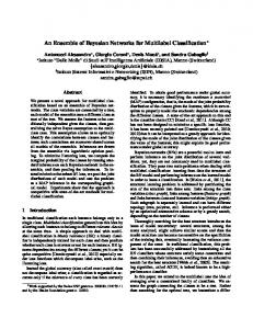
presented results are obtained by using radius distance time series as described earlier. We performed similar experiments using local neighborhood curvature and found similar results which are not shown here. B. Rear View Data Collection We collected video data of passing vehicles using a Sony HDR-SR12 Video Camera. The videos are taken in the early afternoon with sunny and partly cloudy conditions. Lossless compressed PNG image files are extracted from the original HD MPEG4 AVC/H.264 video format, then downsampled from 1440 × 1080 to 320 × 240 using bicubic interpolation. Downsampling is performed to reduce the computation time. All image frames were manually labeled with the vehicle class to provide the ground-truth for evaluation purposes. Figure 11 shows three examples for each known vehicle class. The number in front of the class label denotes the difficulty level of classifying that case (e.g., Sedan 3 (Fig. 11(c)) is harder to classify than Sedan 1 (Fig. 11(a))). The dataset consists of 100 sedans, 27 pickup trucks, and 42 SUV/minivans. We have not added more SUV and pickup images to the database because the current number of samples for each class in the database reflects the actual distribution of vehicle classes at our data capture location. Before extracting the features and generating the feature set, it’s important to determine the number of frames required for classification. We recorded classification accuracy for different number of frames. The maximum accuracy is achieved when 5 frames are used. Note that these frames are not successive. We are using ∆t = 2 which means leaving out two frames between candidate frames. This value is directly related to the speed of the vehicle and the overall time the vehicle is visible in the camera’s field of view. Although currently a predetermined value is used for ∆t, we plan to automatically determine the optimal value as part of future work. To evaluate how well the algorithm performs in the case of an unknown vehicle we also collected 8 unknown vehicles which are not part of the training dataset. Figure 12 shows two examples of unknown vehicles. Figure 10 shows the corresponding pattern-feature matrix. The y-axis represents the extracted features and the x-axis symbolizes all 845 (169 vehicles × 5 frames) feature vectors. For presentation purposes each row has been normalized by dividing by the maximum value of the same feature.


7

Fig. 10.

Pattern-Feature matrix for different vehicles

average testing time per frame from 0.05 to 0.03 seconds. The selected feature numbering is according to the features listed in Section III-A.4. TABLE III F EATURE S ELECTION R ESULTS (a) Sedan 1

(b) Sedan 2

(c) Sedan 3 FS Method↓ (a) None (b) SFFS

. (d) Pickup 1

(e) Pickup 2

(f) Pickup 3

(g) SUV 1

(h) SUV 2

(i) SUV 3

Fig. 11.

Selected features all 1,4,6,10,11

Precision 95.68 94.23

FA Rate 0.02 0.03

CCR 97.63 96.68

Testing time(s) 0.05 0.03

D. Classification Results We use the Bayes Net Toolbox (BNT) [28], an open source Matlab package, for defining the DBN structure, parameter learning, and computing the marginal distribution on the class node. The proposed classification system was tested on our dataset consisting of 169 known and 8 unknown vehicles. We use stratified k-fold cross-validation with k = 10 to evaluate our approach. The resulting confusion matrix is shown in Table IV. All sedans are correctly classified except for the TABLE IV C ONFUSION M ATRIX

Known vehicle examples for each class Pred. Class → True Class↓ Unknown Sedan Pickup SUV/Minivan

Fig. 12.

Unknown vehicle examples

C. Feature Selection Evaluation Table III shows classification evaluation metrics both when (a) using the entire feature set, and (b) using a suboptimal subset. Results show that using the subset of the features generated by SFFS decreases the accuracy and precision by approximately 1%. Feature selection also decreases the

Unknown

Sedan

Pickup

8 0 0 0

0 99 0 3

0 1 27 2

SUV/ Minivan 0 0 0 37

Total 8 100 27 42

one which is misclassified as a pickup truck (Figure 13(a)). Figure 13(b) shows an SUV misclassified as a pickup truck. A closer look at the data and pattern-feature matrix shows great similarity for both these cases with the pickup class due to the license plate location and rear tail light width. E. Structure Learning Evaluation Table V presents the classification evaluation metrics for the two structures given in Figure 8(a) and Figure 8(b). The results show that learning the structure using K2 decreases the classification accuracy and precision. This is due to the fact that the K2 search algorithm requires a known linear


8

TABLE VIII P RECISION PERCENTAGES COMPARISON

(a) Sedan misclas- (b) SUV misclas- (c) Minivan mis- (d) Minivan missified as pickup sified as pickup classified as sedan classified as sedan Fig. 13.

Misclassified examples

ordering of nodes prior to model selection. One way to overcome this is to determine the ordering of nodes prior to performing K2. Determining the required ordering using a dynamic programming approach takes O(n2 2n ) time and O(n2n ) space where n is the number of nodes. The linear order determines the possible parent candidates for each node in a way that the BN is guaranteed to be an acyclic graph.

Classifier→ Vehicle Class↓ Sedan Pickup SUV/Minivan Overall

kNN

LDA

SVM

HDBN

88.46 80.64 85.29 84.80

95.05 78.13 91.67 88.28

96.07 86.20 87.17 89.81

97.05 90.00 100 95.68

than the other classifiers discussed here. Another interesting fact is related to each classifiers performance on the features. On our dataset, HDBN tends to be a more accurate classifier when features are not linearly separable (e.g., feature 8).

TABLE V S TRUCTURE L EARNING E VALUATION Structure Learning Method K2 algorithm & BIC (Figure 8(a)) Manual chosen structure (Figure 8(b))

Precision 93.68 95.68

FA Rate 0.04 0.02

CCR 96.06 97.63

F. Comparison with Other Methods We compare our results with 3 well-known classifiers: knearest neighbor (kNN), linear discriminant analysis (LDA), and support vector machines (SVM). All classification algorithms use the same feature set as the HDBN classifier. Tables VI, VII, and VIII show classification accuracy, false positive ratio (false alarm), and precision respectively. The class ‘unknown‘ is not included in computing the results for Tables VI, VII, and VIII.

Fig. 14.

Feature CCR Contribution Comparison

Figure 15 presents the Receiver Operating Characteristic (ROC) curves for all the four classifiers. Although the ROC curves are similar but it is clear that HDBN out performs SVM, LDA, and KNN.

TABLE VI CCR COMPARISON FOR K NN, LDA, SVM, AND HDBN Classifier→ Vehicle Class↓ Sedan Pickup SUV/Minivan Overall

kNN

LDA

SVM

HDBN

88.25 95.12 90.90 91.42

94.67 94.67 92.89 94.07

96.44 96.44 92.30 95.06

97.63 98.22 97.04 97.63

TABLE VII FALSE ALARM PERCENTAGES COMPARISON Classifier→ Vehicle Class↓ Sedan Pickup SUV/Minivan Overall

kNN

LDA

SVM

HDBN

0.17 0.04 0.04 0.09

0.07 0.05 0.02 0.05

0.06 0.03 0.04 0.04

0.04 0.02 0 0.02

Figure 14 demonstrates how each feature individually contributes to the CCR for all four classifiers kNN, LDA, SVM, and the proposed HDBN. Each bar indicates how much on average the corresponding feature increases/decrease the CCR. The experiment shows that when using HDBN every feature has a positive contribution, whereas for the other three classifiers particular features may decrease the CCR (e.g., feature for kNN, feature 8 for kNN, LDA, and SVM). This observing shows that HDDN is more tolerant to unreliable/noisy features

Fig. 15.

Performance ROC plot

V. C ONCLUSIONS We proposed a Dynamic Bayesian Network for vehicle classification and showed that using multiple video frames in a DBN structure can outperform well known classifiers such as kNN, LDA, and SVM. Our experiments showed that obtaining high classification accuracy does not always require high level features and simple features (e.g., normalized distance and angle) may also provide such results making it possible to perform real-time classification. Future work will involve converting the current training-testing model to an incremental online learning model, stochastic vehicle make and model identification, and adaptive DBN structure learning for classification purposes.


R EFERENCES [1] Y. Shan, H. Sawhney, and R. Kumar, “Unsupervised learning of discriminative edge measures for vehicle matching between nonoverlapping cameras,” IEEE Transactions on Pattern Analysis and Machine Intelligence, vol. 30, no. 4, pp. 700–711, Apr. 2008. [2] T. Lim and A. Guntoro, “Car recognition using Gabor filter feature extraction,” in Asia-Pacific Conference on Circuits and Systems. APCCAS ’02, vol. 2, 2002, pp. 451–455. [3] W. Wu, Z. QiSen, and W. Mingjun, “A method of vehicle classification using models and neural networks,” in IEEE VTS 53rd Vehicular Technology Conference, VTC ’01, vol. 4, 2001, pp. 3022–3026. [4] X. Ma and W. Grimson, “Edge-based rich representation for vehicle classification,” in Tenth IEEE International Conference on Computer Vision, ICCV ’05, vol. 2, Oct. 2005, pp. 1185–1192. [5] M.-P. Dubuisson Jolly, S. Lakshmanan, and A. Jain, “Vehicle segmentation and classification using deformable templates,” IEEE Transactions on Pattern Analysis and Machine Intelligence, vol. 18, no. 3, pp. 293– 308, Mar. 1996. [6] S. Khan, H. Cheng, D. Matthies, and H. Sawhney, “3D model based vehicle classification in aerial imagery,” in IEEE Conference on Computer Vision and Pattern Recognition, CVPR ’10, June 2010, pp. 1681–1687. [7] J. Prokaj and G. Medioni, “3D model based vehicle recognition,” in Workshop on Applications of Computer Vision, WACV., 2009, pp. 1–7. [8] J. Wu and X. Zhang, “A PCA classifier and its application in vehicle detection,” in Proceedings of International Joint Conference on Neural Networks, 2001. IJCNN ’01., vol. 1, 2001, pp. 600–604. [9] M. Conos, “Recognition of vehicle make from a frontal view,” Master’s thesis, Czech Tech. Univ., Prague, Czech Republic, 2006. [10] A. Psyllos, C. N. Anagnostopoulos, and E. Kayafas, “Vehicle model recognition from frontal view image measurements,” Computer Standard Interfaces, vol. 33, pp. 142–151, Feb. 2011. [11] L. Dlagnekov and S. Belongie, “Recognizing cars,” UCSD, Tech. Rep. CS2005-083, 2005. [12] Z. Chen, N. Pears, M. Freeman, and J. Austin, “Road vehicle classification using support vector machines,” in IEEE International Conference on Intelligent Computing and Intelligent Systems, ICIS 2009, vol. 4, Nov. 2009, pp. 214–218. [13] D. Zhang, S. Qu, and Z. Liu, “Robust classification of vehicle based on fusion of tsrp and wavelet fractal signature,” in IEEE Conf. on Networking, Sensing and Control, ICNSC., 2008, pp. 1788–1793. [14] Y.-L. Chen, B.-F. Wu, H.-Y. Huang, and C.-J. Fan, “A real-time vision system for nighttime vehicle detection and traffic surveillance,” IEEE Trans. on Industrial Electronics, vol. 58, pp. 2030–2044, May 2011. [15] X. Cao, C. Wu, J. Lan, P. Yan, and X. Li, “Vehicle detection and motion analysis in low-altitude airborne video under urban environment,” IEEE Transactions on Circuits and Systems for Video Technology, vol. 21, no. 10, pp. 1522–1533, Oct. 2011. [16] F. Alves, M. Ferreira, and C. Santos, “Vision based automatic traffic condition interpretation,” in 8th IEEE International Conference on Industrial Informatics, INDIN 2010, July 2010, pp. 549–556. [17] M. Chacon and S. Gonzalez, “An adaptive neural-fuzzy approach for object detection in dynamic backgrounds for surveillance systems,” IEEE Transactions on Industrial Electronics, vol. PP, no. 99, p. 1, 2011. [18] S. Nadimi and B. Bhanu, “Multistrategy fusion using mixture model for moving object detection,” in International Conf. on Multisensor Fusion and Integration for Intelligent Systems, MFI 2001., 2001, pp. 317–322. [19] G. Loy and J. olof Eklundh, “Detecting symmetry and symmetric constellations of features,” in ECCV, 2006, pp. 508–521. [20] S. Nadimi and B. Bhanu, “Physical models for moving shadow and object detection in video,” IEEE Transactions on Pattern Analysis and Machine Intelligence, vol. 26, pp. 1079–1087, 2004. [21] W.-Y. Ho and C.-M. Pun, “A Macao license plate recognition system based on edge and projection analysis,” in 8th IEEE International Conference on Industrial Informatics, INDIN, July 2010, pp. 67–72. [22] C. Anagnostopoulos, I. Anagnostopoulos, V. Loumos, and E. Kayafas, “A license plate-recognition algorithm for intelligent transportation system applications,” IEEE Transactions on Intelligent Transportation Systems, vol. 7, no. 3, pp. 377–392, Sept. 2006. [23] V. Abolghasemi and A. Ahmadyfard, “An edge-based color-aided method for license plate detection,” Image and Vision Computing, vol. 27, pp. 1134–1142, July 2009. [24] C. Paulo and P. Correia, “Automatic detection and classification of traffic signs,” in Eighth International Workshop on Image Analysis for Multimedia Interactive Services, WIAMIS ’07, June 2007, p. 11. [25] Y. Guo, C. Rao, S. Samarasekera, J. Kim, R. Kumar, and H. Sawhney, “Matching vehicles under large pose transformations using approximate 3D models and piecewise MRF model,” IEEE Conference on Computer Vision and Pattern Recognition, CVPR ’08, pp. 1–8, 2008. [26] N. Otsu, “A threshold selection method from gray-level histograms,” IEEE Transactions on Systems, Man and Cybernetics, vol. 9, no. 1, pp. 62–66, Jan. 1979.

9

[27] H. Sakoe and S. Chiba, “Dynamic programming algorithm optimization for spoken word recognition,” IEEE Transactions on Acoustics, Speech and Signal Processing, vol. 26, no. 1, pp. 43–49, Feb. 1978. [28] K. P. Murphy, “The Bayes net toolbox for MATLAB,” in Computing Science and Statistics: Proceedings of the Interface, vol. 33, 2001. [Online]. Available: http://code.google.com/p/bnt/

Mehran Kafai (S’11) received the B.S degree in computer engineering from the Bahonar university, Kerman, Iran, in 2002, the M.S. degree in computer engineering from the Sharif university of technology, Tehran, Iran, in 2005, and the M.S degree in computer science from the San Francisco state university in 2009. He is currently working toward the Ph.D. degree in computer science at the Center for Research in Intelligent Systems in the University of California, Riverside. His research interests are in computer vision, pattern recognition, machine learning, and data mining. His recent research has been concerned with robust object recognition algorithms. Bir Bhanu (S’72-M’82-SM’87-F’95) received the S.M. and E.E. degrees in electrical engineering and computer science from the Massachusetts Institute of Technology, Cambridge, the Ph.D. degree in electrical engineering from the Image Processing Institute, University of Southern California, Los Angeles, and the MBA degree from the University of California, Irvine. Dr. Bhanu is the Distinguished Professor of Electrical Engineering and serves as the Founding Director of the interdisciplinary Center for Research in Intelligent Systems at the University of California, Riverside (UCR). He was the founding Professor of electrical engineering at UCR and served as its first chair (1991-94). He has been the cooperative Professor of Computer Science and Engineering (since 1991), Bioengineering (since 2006), Mechanical Engineering (since 2008) and the Director of Visualization and Intelligent Systems Laboratory (since 1991). Previously, he was a Senior Honeywell Fellow with Honeywell Inc., Minneapolis, MN. He has been with the faculty of the Department of Computer Science, University of Utah, Salt Lake City, and with Ford Aerospace and Communications Corporation, Newport Beach, CA; INRIA-France; and IBM San Jose Research Laboratory, San Jose, CA. He has been the principal investigator of various programs for the National Science Foundation, the Defense Advanced Research Projects Agency (DARPA), the National Aeronautics and Space Administration, the Air Force Office of Scientific Research, the Office of Naval Research, the Army Research Office, and other agencies and industries in the areas of video networks, video understanding, video bioinformatics, learning and vision, image understanding, pattern recognition, target recognition, biometrics, autonomous navigation, image databases, and machine-vision applications. He is coauthor of the books Computational Learning for Adaptive Computer Vision (Forthcoming), Human Recognition at a Distance in Video (SpringerVerlag, 2011), Human Ear Recognition by Computer (Springer-Verlag, 2008), Evolutionary Synthesis of Pattern Recognition Systems (Springer-Verlag, 2005), Computational Algorithms for Fingerprint Recognition (Kluwer, 2004), Genetic Learning for Adaptive Image Segmentation (Kluwer, 1994), and Qualitative Motion Understanding (Kluwer, 1992), and coeditor of the books on Computer Vision Beyond the Visible Spectrum (Springer-Verlag, 2004), Distributed Video Sensor Networks (Springer-Verlag, 2011), and Multibiometrics for Human Identification (Cambridge University Press, 2011). He is the holder of 18 (5 pending) U.S. and international patents. He has more than 350 reviewed technical publications, including over 100 journal papers. He has been on the editorial board of various journals and has edited special issues of several IEEE TRANSACTIONS (PATTERN ANALYSIS AND MACHINE INTELLIGENCE; IMAGE PROCESSING; SYSTEMS, MAN AND CYBERNETICS-PART B; ROBOTICS AND AUTOMATION; INFORMATION FORENSICS AND SECURITY) and many other journals. He was the General Chair for the IEEE Conference on Computer Vision and Pattern Recognition, the IEEE Conference on Advanced Video and Signal-based Surveillance, the IEEE Workshops on Applications of Computer Vision, the IEEE Workshops on Learning in Computer Vision and Pattern Recognition; the Chair for the DARPA Image Understanding Workshop, the IEEE Workshops on Computer Vision Beyond the Visible Spectrum and the IEEE Workshops on Multi-Modal Biometrics. He was the recipient of best conference papers and outstanding journal paper awards and the industrial and university awards for research excellence, outstanding contributions, team efforts and doctoral/dissertation advisor/mentor award. Dr. Bhanu is a Fellow of the IEEE, the American Association for the Advancement of Science, the International Association of Pattern Recognition, and the International Society for Optical Engineering.