Dec 2, 2004 - arXiv:cond-mat/0412053v1 [cond-mat.stat-mech] 2 Dec 2004. Dynamics of ... Everyday, transportation networksâ airports, roads, the Internet, etcâ ..... becomes very large and eventually diverge when h â 1. In conclusion, we ...
Dynamics of jamming transitions in complex networks Pablo Echenique,1, 2 Jes´ us G´omez-Garde˜ nes,3, 2 and Yamir Moreno2, 1
arXiv:cond-mat/0412053v1 [cond-mat.stat-mech] 2 Dec 2004
1
Departamento de F´ısica Te´ orica, Universidad de Zaragoza, Zaragoza 50009, Spain. 2 Instituto de Biocomputaci´ on y F´ısica de Sistemas Complejos, Universidad de Zaragoza, Zaragoza 50009, Spain 3 Departamento de F´ısica de la Materia Condensada, Universidad de Zaragoza, Zaragoza 50009, Spain (Dated: February 2, 2008)
We numerically investigate jamming transitions in complex heterogeneous networks. Inspired by Internet routing protocols, we study a general model that incorporates local traffic information through a tunable parameter. The results show that whether the transition from a low-traffic regime to a congested phase is of first or second order type is determined by the protocol at work. The microscopic dynamics reveals that these two radically different behaviors are due to the way in which traffic jams propagate through the network. Our results are discussed in the context of Internet dynamics and other transport processes that take place on complex networks and provide insights for the design of routing policies based on traffic awareness in communication systems. PACS numbers: 89.75.-k, 89.75.Fb, 89.20.-a, 89.20.Hh
Everyday, transportation networks− airports, roads, the Internet, etc− carry on a huge amount of load in the form of passengers, vehicles or information packets delivered by millions of users when searching the World-WideWeb (WWW), sending and receiving e-mails, or looking at stock market quotes. The globalization and the Information Era have in turn led to a continuous growth of most communication networks driven by the increase in traffic; capital examples being the Internet and main airports. The efficient performance of these systems is mainly determined by the ability of the system to avoid congestion and reduce transit times. Congestion on networked systems often comes up suddenly and provokes the breakdown of the system’s functionality. Hence, it is not surprising that transport processes and information exchange have been widely studied over the last years because of potential applications in fields as diverse as sociology [1], urban planning (vehicular traffic) [2, 3], informatics [4, 5, 6, 7, 8] and biology [9]. A great body of work in the subject has been carried out for regular and random graphs. Real networks are however complex. The patterns of interconnections describing the interactions of the system’s elements have been unraveled just a few years ago. Surprisingly, in sharp contrast with the common sense, systems as diverse as the Internet, the WWW, biological and social networks [10, 11, 12] share a number of topological features. This fact makes the modeling of complex networks an attractive field as one may define and study general models and then translate the conclusions and implications to the language of a particular field. For instance, the resilience to random failures and attacks and the spreading of virus and rumors [13, 14, 15, 16, 17, 18] are relevant problems in sociology, biology and technological systems. The intense research on complex networks during the last years have provided deep insights into the dependency of the properties of dynamical processes on the
topological properties of the underlying networks in which these processes take place. Of particular interest are the so-called scale-free (SF) networks [19], since they have been shown to radically change well-established results for random graphs and regular lattices. These networks are ubiquitous in Nature. They are made up of a number of nodes (or elements) and the probability that a given node has k connections to other nodes follows a power law Pk ∼ k −γ . This is the case of the Internet which shows a scale-free (SF) connectivity distribution with an exponent that has been estimated to be around γ = 2.2 [13]. In this paper, we study the impact of traffic routing protocols on the performance of communication systems when traffic awareness is incorporated. More specifically, we are interested in exploring how the average network performance depends on the ability of the routing protocol to divert traffic across paths other than the shortest ones. To this end, we numerically explore a model in which a tunable parameter accounts for the degree of traffic awareness incorporated in packets delivery. We find that the onset of the congested phase is reminiscent of a first or a second order phase transition depending on whether or not the routing combines a shortest path delivery strategy with traffic aggregation at a local scale. We also report on the differences in local dynamics and discuss our results in the context of cost-performance trade-offs associated with different routing strategies. In order to be more precise, we shall discuss in what follows our model and results within the field of technological networks such as the Internet. However, as we will see, the model is aimed at simulating a general transport process on top of a complex scale-free network. Hence, our results could also be useful in other fields. Moreover, as it was recently shown [8], different routing strategies are sensitive to local details of the networks under study− for instance, to the degree-degree correlations and the clustering coefficient−, so that it is advisable to
2
δi = hdi + (1 − h)ci ,
4
10
3
(a)
2
A
10
1
10
0
0
50 100 150 200
4
10
0
2000
4000
4
10
(c)
3
(d)
3
10
1
10
A
4
10
2
0
(b)
10
A
100 80 60 40 20 0
A(x10 )
use real networks. Hence, we have used the Internet Autonomous System map at the Oregon route server dated May 25, 2001 [20], which is a SF network with γ = 2.2 and N = 11174 nodes. The model is defined as follows. Starting from an unloaded network, we impose a constant input of newly created packets. At each time step, p information packets are created. The source of each packet as well as its destination are chosen at random among all the nodes of the network. Besides, each node sends only one packet at each time step and, as a consequence, one node, i, can have a queue of ci packets to be delivered. The pathdelivery strategy is sketched below. Let us suppose that a node l is holding a packet whose destination is j. Then, the effective distance between a neighbor i (i = 1, . . . , kl ) of l and j is defined as
2 1 0
0
10 2000 4000 6000 0 t
2000 4000 6000 t
(1)
where di is the minimum number of hops one has to pass by in order to reach j, i.e., the shortest path between i and j. Additionally, h is a tunable parameter that accounts for the degree of traffic awareness incorporated in the delivery algorithm. It is worth noting that when h = 1, we recover a shortest-path delivery protocol similar to actual Internet routing mechanisms− in the Internet, routers deliver data packets by converging to a best estimate of the path connecting each destination address− or to the typical behavior in urban traffic. The packet is finally diverted following the path going through the node that minimizes δi . Henceforth, we will distinguish between the case h = 1, referred to as standard protocol, and h 6= 1, called traffic-aware scheme. Other strategies are also possible [8], but it has been recently shown that the two described above give the best network’s performance when packets are only introduced at the beginning of the process. The procedure for h 6= 1 combines knowledge of the structural properties of the network and its current dynamical state at a local scale. It allows to divert packets through larger but less congested paths, consequently a trade-off associated to packets’ transit times is naturally and dynamically incorporated. As an appropriate measure of the efficiency of the process, we monitor the aggregation of packets in the network, given by the number of packets that have not reached their destinations at each time step t, A(t). Figure 1 shows the results obtained for different values of p and h. As it can be seen, when the external driving is applied at low rates (i.e., small p), both protocols allow for a stationary state. In this state, the system is able to balance the in-flow of packets with the flow of packets that reach their destinations. The stationary state, where no macroscopic signs of congestion is observed, corresponds to a free flow phase. The situation changes when the rate at which new packets are introduced increases. As we will see below, there is a critical value pc beyond which a congested phase shows up. Let us now note that for the standard protocol (Fig. 1a, dotted line), when p > pc , A(t) grows linearly in time
FIG. 1: Total number of active packets as a function of time steps. Figures (a) and (b) correspond to the standard protocol, while (c) and (d) have been obtained for the traffic-aware routing with h = 0.85. In each figure, the continuous line stand for subcritical values of p ((a) and (b) p = 3.0, (d) p = 8.0) and the dotted line corresponds to p > pc ((a) and (b) p = 4.0, (c) and (d) p = 13.0). See the text for further details on the definitions.
∀t. On the contrary, for the traffic-aware algorithm, we observe that A(t) grows slowly at short times and then becomes steeper as time goes on with a constant slope (Fig. 1c). In order to characterize the phase transition from a free phase to a congested one, we introduce the order parameter ρ = lim
t→∞
A(t + τ ) − A(t) , τp
(2)
where τ is the observation time. The limit in Eq. (2) is introduced only to ensure that the system is not in a temporary regime. Equation (2) hence measures the ratio between the outflow and the inflow of packets during a time window τ . ρ equals 1 when the congestion is maximal (no packet reaches its destination) and 0 when an equilibrium is established, i.e., in the stationary state. Figure 2 depicts the system’s phase diagram. The dynamics of the system is characterized in both protocols by a critical point beyond which a macroscopic congestion arises. However, there are two radically different behaviors for the onset of traffic jams. In the standard protocol (h = 1), the critical point is small, pc = 3 and the jamming transition is reminiscent of a second order phase transition. On the contrary, when h 6= 1, the critical point pc ≈ 9 is distinctly larger than for h = 1, but the appearance of a congested phase turns out to be consistent with a first order phase transition, with a sharp jump of ρ at the transition point. Moreover, the order of the transition for the latter protocol is independent of h
3
h=0.85
1.0
h=1.00
0.8
ρ
T
0.6
0.4
h=1 h=0.95 h=0.75 h=0.5
0.2
0.0
0
5
10
15 p
20
25
30
FIG. 2: Jamming transitions as a function of p. The order parameter ρ is given by Eq. (2). Note that h = 1 corresponds to the standard strategy in which traffic awareness is absent. As soon as traffic conditions are taken into account, the jamming transition is reminiscent of a first-order phase transition and the critical point shifts rightward.
provided that h 6= 1. The two different types of transitions depending on whether or not traffic-awareness is incorporated in the protocol at work, poses an interesting issue. Which of the two protocols will be best suited to handle traffic? It depends on the system. While for the standard protocol we get a smaller critical point, the jammed phase does not appear suddenly. Hence, if we would like to have a system in which traffic jams appear and grow smoothly, the standard algorithm is the best choice. On the contrary, we could implement a sort of traffic-aware protocol if we are interested in delaying the appearance of congestion, however at the cost of a sudden jump to a highly jammed phase due to the lack of previous warnings. In order to provide more insights into the nature of the phase transitions, we now focus on the microscopic details of the system’s dynamics. We have inspected how the nodes get congested. As both protocols incorporate a shortest path delivery strategy, a suitable description can be obtained by monitoring the number of active packets at each node as a function of the betweenness of the nodes− which, on the other hand, scales with k [13]. The betweenness or load of a node i gives the total number of shortest paths among all pairs of nodes in the network that pass through i [13, 21, 22]. It is a measure of the centrality of a node in the network and becomes a relevant quantity in traffic flow modeling. Figure 3 clearly illustrates the distribution of congested vertices for the two protocols analyzed. The shortest paths connecting the sources and the destinations of any active packet always tend to visit first the more connected nodes and then go down to the less connected ones. This is a consequence of the hierarchy of the network and is called up-down
ln(B)
FIG. 3: (Color online) Congestion levels as a function of time and nodes’ betweenness. At each time step, the color-coded scale is normalized by the number of packets ci in the queue of the node with the largest congestion. Two radically distinct behaviors are obtained for the standard (h = 1, p = 4 > pc = 3, right panel) and the traffic-aware (h = 0.85, p = 13 > pc = 9, left panel) protocols.
strategy [13]. For h = 1, the protocol only works on a shortest path delivery basis. The hubs become congested early in the process causing the packets to get trapped in a few nodes as shown in Fig. 3. When traffic conditions are taken into account by the routing mechanisms, the same up-down strategy applies up to the hubs. Then, instead of getting trapped in them, the packets circumvent highly jammed nodes and the load is distributed to nodes other than the hubs, provoking the aggregation of traffic in neighborhoods of overcrowded nodes. In the long time limit, the congestion is spread through the network (see, Fig. 3) shifting the critical point to larger values of p. It is possible to get deeper into what is going on in the system for h 6= 1. Let us suppose again that a node l is holding a packet to be sent to j through one of its neighbors i (i = 1, . . . , kl ). Among all the neighbors of l, there is one node with the lowest load cmin . Now, assume the extreme situations in which by going through i the packet is one hop closer to its destination, but taking the path for which ci = cmin , it is one hop farther from j. Thus it follows that whenever the relation ci − cmin > 2h/(1 − h) is verified, the packet will never be sent through i. This node i is impenetrable for l. If a node is impenetrable for all its neighbors, we call it just impermeable, since it does not participate in traffic delivery. As congestion spreads throughout the network, the number of impermeable nodes increases and changes dynamically. Therefore a dynamical backbone made up of all nodes that are able
4 1.0
/Gmax, A
0.8 /Gmax
0.6
A
0.4
0.2
0.0
0
10000
20000 t
30000
40000
FIG. 4: Time dependence of the total number of packets in the system and average size of the clusters formed by non impermeable nodes. Note that A(t) becomes steeper just when the inflection of hGi/Gmax (t) changes. h = 0.85 and p = 13. See the text for further details.
to transmit the packets comes up. The picture is similar to the percolation of a fluid through a porous media. Here, packets can flow only through non impermeable nodes as a fluid can only flow through the pore channels. The existence of impermeable nodes provokes the appearance of both small network components in the form of impenetrable regions, and clusters of allowed paths. Figure 4 depicts the time dependence of the average cluster size (normalized by the largest cluster size) of allowed regions. Starting from t = 0, as time goes on, the total number of packets in the network increases and there is only one cluster of the size of the network. When signs of congestion first appear, hGi/Gmax (t) decreases departing from unity. At longer times, traffic jams reach more nodes (see, Fig. 3, for t > 21000) causing the congestion to be more distributed in the network. Finally, the flow of packets in the network reaches a regime in which A(t)
[1] D. J. Watts and S. H. Strogatz, Nature 393, 440 (1998). [2] K. Nagel and M. Schreckenberg, J. Phys. A 26, L679 (1993). [3] K. Nagel and M. Paczuski, Phys. Rev. E 51 2909, 1995. [4] T. Ohira abd R. Sawatari, Phys. Rev. E 58 193, 1998. [5] M. Takayasu, H. Takayasu and K. Fukuda, Physica A 277, 248 (2000). [6] R. Guimera, A. Arenas, A. D´ıaz-Guilera, and F. Giralt, Phys.Rev. E 66, 026704 (2002). [7] S. Valverde and R. V. Sol´e, Physica A 312, 636 (2002); Eur. Phys. J. B 38, 245 (2004). [8] P. Echenique, J. G´ omez-Garde˜ nes, and Y. Moreno, Phys. Rev. E 70, 056105 (2004). [9] M. Tlalka et al, New Phytologist 158, 325 (2003). [10] S. H. Strogatz, Nature (London) 410, 268 (2001).
increases linearly in time and ρ saturates to its stationary value. In this state, marked by an inflection point in the hGi/Gmax (t) curve beyond which the average cluster size of allowed regions stabilizes, the system seems to have self-organized the distribution of jammed nodes. This self-organization phenomenon nicely explains why one can not go from one protocol to the other by making h = 1, as it can seem from Eq. (1). The discontinuity at h = 1 is therefore due to the lack of alternative paths in the standard protocol. Even for h very close to 1, the system will self-organize itself into a state in which congested nodes are distributed and not limited to the very hubs of the network. The only dependence with h is manifested in the time needed for self-organization, that becomes very large and eventually diverge when h → 1. In conclusion, we have characterized jamming transitions in complex heterogeneous networks. The results show that when traffic awareness is incorporated into the routing protocol, new cooperative effects arise. Additionally, the jamming transitions are well described by two radically different phase transitions. Finally, our results demonstrate that whether or not a given protocol is best suited for traffic handling depends on a delicate trade-off between the system’s performance and traffic capabilities (how large pc is) and how congestion arises (smoothly or suddenly). The model thus provides useful insights for the design of new routing policies and may be a guide for more complex models where, for instance, routers can tune h dynamically depending on the traffic conditions at a local scale.
Acknowledgments
P. E. and J. G-G acknowledge financial support of the MECyD through FPU grants. Y. M. is supported by MEyC through the Ram´ on y Cajal Program. This work has been partially supported by the Spanish DGICYT projects BFM2002-01798 and BFM2002-00113.
[11] S. N. Dorogovtsev and J. F. F. Mendes, Evolution of Networks. From Biological Nets to the Internet and the WWW, Oxford University Press, Oxford, U.K., (2003). [12] Handbook of Graphs and Networks, Edited by S. Bornholdt and H. G. Schuster, Wiley-VCH, Germany, 2003. [13] R. Pastor-Satorras and A. Vespignani, Evolution and Structure of the Internet, Cambridge University Press, Cambridge, U.K., (2004). [14] R. Cohen, K. Erez, D. ben-Avraham, and S. Havlin, Phys. Rev. Lett. 85, 4626 (2000); [15] D. S. Callaway, M. E. J. Newman, S. H. Strogatz, and D. J. Watts, Phys. Rev. Lett. 85, 5468 (2000). [16] Y. Moreno, R. Pastor-Satorras, and A. Vespignani, Eur. Phys. J. B 26, 521 (2002). [17] A. V´ azquez, and Y. Moreno, Phys. Rev. E 67, 015101(R)
5 (2003). [18] M. E. J. Newman, Phys. Rev. E 66, 016128 (2002). [19] A.-L. Barab´ asi, and R. Albert, Science 286, 509 (1999). [20] Available at http://topology.eecs.umich.edu/. Electric Engineering and Computer Science Department, Univer-
sity of Michigan, Topology Project. [21] M. E. J. Newman, Phys. Rev. E 64, 016132 (2001). [22] K. Goh et al, Phys. Rev. Lett. 87, 278701 (2001).


![Phase Transitions in Complex Networks [PDF]](https://m.moam.info/img/260x300/phase-transitions-in-complex-networks-pdf_64966fce098a9e09098b4596.jpg)