developed similar type of projects and the training data consisting of software measurements. To predict faulty modules in software data different techniques ...
2009 Second International Conference on Machine Vision
Early Software Fault Prediction using Real Time Defect Data Arashdeep Kaur Deptt. Of CSE Amity University, Noida, India
Parvinder S. Sandhu
Amanpreet Singh Brar
Deptt. Of CSE Rayat & Bahra Institute of Engg.& BioTechnology,Mohali, India
Dept.of CSE, Guru Nanak Dev Engg. College Ludhiana, India
Abstract— Quality of a software component can be measured in terms of fault proneness of data. Quality estimations are made using fault proneness data available from previously developed similar type of projects and the training data consisting of software measurements. To predict faulty modules in software data different techniques have been proposed which includes statistical method, machine learning methods, neural network techniques and clustering techniques. The aim of proposed approach is to investigate that whether metrics available in the early lifecycle (i.e. requirement metrics), metrics available in the late lifecycle (i.e. code metrics) and metrics available in the early lifecycle (i.e. requirement metrics) combined with metrics available in the late lifecycle (i.e. code metrics) can be used to identify fault prone modules by using clustering techniques. This approach has been tested with three real time defect datasets of NASA software projects, JM1, PC1 and CM1. Predicting faults early in the software life cycle can be used to improve software process control and achieve high software reliability. The results show that when all the prediction techniques are evaluated, the best prediction model is found to be the fusion of requirement and code metric model.
using different programming language constructs resulting in different static measures for that module. Fenton uses this example to argue the uselessness of static code attributes [4]. Therefore, using static features alone can be uninformative. A module currently under development is fault prone if a module with the similar product or process metrics in an earlier project developed in the same environment was fault prone. Therefore, the information available early within the current project or from the previous project can be used in making predictions. Although requirements metrics alone are not best at finding the faults but these metrics can increase the performance prediction. It is required that fault-prone prediction models should be efficient and accurate. Thus, combinations of static features extracted from requirements and code can be exceptionally good predictors for identifying modules that actually contains faults. [2] To predict the fault in software data a variety of techniques have been proposed which includes statistical method, machine learning methods, neural network techniques and clustering techniques. Much of the work has done on checking the quality with statistical methods and machine learning methods using either requirement or static code metrics. But very few have worked on finding the faulty and non faulty modules by using clustering techniques. However, estimating the quality using clustering techniques on fusion of requirement and code metric has not been proposed in the literature. Prediction of fault-prone modules provides one way to support software quality engineering through improved scheduling and project control.
Keywords- Clustering, K-means, Defect data, ROC curve and software quality. I.
INTRODUCTION
A software fault is a defect that causes software failure in an executable product. In software engineering, the nonconformance of software to its requirements is commonly called a bug. Software Engineers distinguish between software faults, software failures and software bugs. In case of a failure, the software does not do what the user expects but on the other hand fault is a hidden programming error that may or may not actually manifest as a failure and the non-conformance of software to its requirements is commonly called a bug. To predict faults different metric measures are available. Metrics available during static code development such as Halstead complexity, McCabe complexity, can be used to check modules for fault proneness. Fenton offers an example where the same program functionality is achieved 978-0-7695-3944-7 2010 U.S. Government Work Not Protected by U.S. Copyright DOI 10.1109/ICMV.2009.54
A. Clustering Algorithms Clustering is an approach that uses software measurement data consisting of limited or no fault-proneness data for analyzing software quality. In this study, K-Means clustering algorithm is being used for predictive models to predict faulty/non faulty modules. K-means classify data in to different k groups, k being a positive integer, based on the attributes or some features. Grouping of data is done on the basis of minimizing sum of squares of distances between data and their cluster centroid. This approach is an iterative scheme which allows classification of data in to faulty and
242
II.
METHODOLOGY
First of all, the data metrics of requirement phase and structural code attributes of software systems has been collected from NASA Metrics Data Program (MDP) data repository [1]. MDP repository contains data of 13 projects out of which only 3 projects data include requirement metrics. These three projects are CM1 (written in C), containing approximately 505 modules, JM1 (written in C++), containing 10878 modules, PC1 (written in C), containing 1107 modules. CM1 is a NASA spacecraft instrument, JM1 is a real time ground system and PC1 is an earth orbiting satellite system. After collecting and refining the data from NASA projects, requirement metrics and module metrics of the above projects have been joined by using inner join method. Clustering is a technique that divides data in to two or more clusters depending upon some criteria. As, in this study data is divided in to two clusters depending upon that whether they are fault free or fault prone. Then, find the suitable algorithm for clustering of the software components into faulty/fault-free systems. Software quality prediction models seek to predict quality factors such as whether a component is fault prone or not. Methods for identifying fault-prone software modules support helps to improve resource planning and scheduling as well as facilitating cost avoidance by effective verification. Such models can be used to predict the response variable which can either be the class of a module (e.g. fault-prone or not fault-prone) or a quality factor (e.g. number of faults) for a module. However various software engineering practices limit the availability of fault proneness data. With its effect supervised clustering is not possible to implement for analyzing the quality of software. This limited fault proneness data can be clustered by using semi supervised clustering. It is a constraint based clustering scheme that uses software engineering expert’s domain knowledge to iteratively create clusters as either fault-free or fault-prone [3]. To predict the results, we have used confusion matrix. The confusion matrix has four categories: True positives (TP) are the modules correctly classified as faulty modules. False positives (FP) refer to fault-free modules incorrectly labeled as faulty. True negatives (TN) are the fault-free modules correctly labeled as such. False negatives (FN) refer to faulty modules incorrectly classified as fault-free modules.
Predicted
TABLE I.
A CONFUSION MATRIX OF PREDICTION OUTCOMES
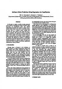
The following set of evaluation measures are being used to find the results: • Probability of Detection (PD), also called recall or specificity, is defined as the probability of correct classification of a module that contains a fault. PD = TP / (TP + FN) (1) • Probability of False Alarms (PF) is defined as the ratio of false positives to all non defect modules. PF = FP / (FP + TN) (2) Basically, PD should be maximum and PF should be minimum [2]. A. ROC Curve ROC is an acronym for Receiver Operator Characteristic; it is a plot of PD versus PF across all possible experimental combinations. ROC analysis is related in a direct and natural way to cost/benefit analysis of software projects by comparing their detected defective and non defective modules. ROC curve provides better insight to comparisons between different parametric values. ROC curve for the described approach is presented in Fig. 1.The values of PD and PF ranges from 0 to 1. The graph is plotted along X-axis and Y-axis ranging from 0 to 1 both. The points plotted in Fig.1 represent the visual comparison of classification performance of predictive models. Typical ROC curve has concave shape with (0, 0) as the beginning and (1, 1) as the end. ROC curve is divided in to four different regions namely, cost adverse region, risk adverse region, negative curve and no information region. In Fig. 1, a straight line connecting (0, 0) and (1, 1) implies that performance of a classifier is no better than random guessing. In the above figure, points named A and B falls in to risk adverse region , it indicates high PD and high PF, this situation is better for safety critical systems, this such performance is preferred because the identification of faults is more important than cost to validate false alarms. In Fig. 1, the points marked A, B, C and D in the ROC curve provides no information regarding the fault proneness of modules. PROBABILITY OF FALSE ALARMS (PF)
non-faulty modules based on Euclidean distance between data points. Finally, ROC Curve has been plotted using the recall value that is used to compare all the three models i.e. static metrics model, requirement metrics model and combination of requirement and code metrics model.
1
E
0.8 F 0.6 0.4 0.2 A,B,C,D
0 0
Real data Fault
No Fault
Fault
TP
FP
No Fault
FN
TN
0.2
0.4
0.6
0.8
1
PROBABILITY OF DETECTION (PD)
Figure1. ROC curve of results
Negative curve in ROC plot comprises data points with low PD and high PF. In software engineering practices, High
243
PD and low PF specify that maximum number of modules has been classified correctly. As the PD decreases and PF increases, the probability that modules can be classified incorrectly increases. But this is not necessarily a bad news because it can be transposed into a preferred curve when classifier negates their tests. III.
are 0 and 0 respectively. These values show that performance is not efficient. Table 3 gives the results of static code metrics models of CM1 and PC1. TP value for CM1 code metrics comes out to be 0, TN is 457, FP is 0 and FN is 48, PD and PF values are 0 and 0 respectively. In the same way, TP value for PC1 code metrics is 0, TN is 1031, FP is 0 and FN is 48, PD and PF values are 0 and 0 respectively. Here PD and PF as 0 indicates that performance is not much better and the results are almost same that of requirement metric model. Hence, these metrics can be effective if they can be combined.
RESULTS & DISCUSSION
The NASA MDP datasets are used in this approach to estimate the quality of a software product. The datasets used are CM1, JM1, and PC1 as these are the only three projects in MDP data repository that include requirement metrics. We used requirement metrics, code metrics and join the requirement and code metrics as specified in [2] for modeling. These prediction models are used with k-means clustering to find the faulty and non faulty modules in a software product and then find the best predictive model among all. The proposed approach has been implemented in MATLAB 7.4. Clustering technique being used is a built-in function in its statistics toolbox. These functions are used with their default parameters. The JM1 dataset is used as a training data to evaluate the quality by calculating the recall value. PC1 and CM1 datasets are used as test data to check which of the three prediction models comes out to be the best to estimate the quality measures using different clustering algorithms, to verify the need for testing, quality assurance. For comparing the results, PD should be maximum and PF should be minimum. These values can range from 0 to 1. TABLE II.
TABLE III.
Evaluation Measures
Projects CM1
PC1
TP
0
0
TN
21
213
FP
0
0
FN
68
107
PD
0
0
PF
0
0
Markers
A
B
Projects CM1
PC1
TP
0
0
TN
457
1031
FP
0
0
FN
48
76
PD
0
0
PF
0
0
Markers
C
D
Table 4 shows the results of the model extracted from requirement and static metrics. The values of TP, TN, FP, FN, PD and PF are 66, 107, 76, 17, 0.99729 and 0.79518 respectively for CM1 dataset. For PC1 dataset TP is 115, TN is 1, FP is 361, FN is 0, PD is 1 and PF is 0.99724.
RESULTS OF REQUIREMENT METRIC MODEL USING KMEANS
Evaluation Measures
RESULTS OF CODE METRICS MODEL USING K-MEANS
TABLE IV.
RESULTS OF FUSION METRIC MODEL USING K-MEANS
Evaluation Measures
Table 2 shows the results of using K-Means clustering on JM1 dataset as training data and using requirement metrics of CM1 and PC1 to calculate their true positives, true negatives, false positives, false negatives, probability of detection and probability of false alarms. TP value for CM1 requirement metrics comes out to be 0, TN is 21, FP is 0 and FN is 67, PD and PF values are 0 and 0 respectively. Similarly, TP value for PC1 requirement metrics comes out to be 0, TN is 213, FP is 0 and FN is 107, PD and PF values
Projects CM1
PC1
TP
66
115
TN
107
1
FP
76
361
FN
17
0
PD
0.99729
1
PF
0.79518
0.99724
Markers
E
F
Therefore, the observed performance here is that real world software engineering situations can be better represented by the training/test datasets after the inner join operations on their requirement and code metrics. The information provided by the static and requirement metrics
244
of all the three datasets is useless for project managers, as only 30% of the modules lie in the exact category either fault free/fault prone. The PD and PF of model derived from combination of requirement and code metrics is far accurate than previously proposed models in literature for production of fault tolerance in software systems. The developed model can be used for classifying a faulty system from non-faulty system on the basis of structural attributes of the software systems. IV.
[3]
[4]
[5]
[6]
CONCLUSION
In this study we predict that knowing the fault prone data at early stages of lifecycle combined with data available during code can help the project managers to build the projects with more accuracy and it will reduce the testing efforts as faulty areas are already predicted, so these modules can be handled properly. The main benefit of using the fusion model is that it gives the more accurate results than the individual models and thus can help to improve the productivity of the product. Data available in the early stages can help the analyst to plan the required resources as and when required for development, testing. As software quality is a vital component of any software development, and these models are being used to achieve improved software quality and accuracy of software projects. However, further investigation can be done and the impact of attributes on the fault prediction can be found. Also, more algorithms can be evaluated and then we can find the best algorithm.
[7]
[8]
[9]
[10]
[11]
[12]
[13]
REFERENCES [1] [2]
NASA IV &V Facility. Metric Data Program. Available from http: //MDP.ivv.nasa.gov/. Jiang Y., Cukic B. and Menzies T. (2007), “Fault Prediction Using Early Lifecycle Data”. ISSRE 2007, the 18th IEEE Symposium on
245
Software Reliability Engineering, IEEE Computer Society, Sweden, pp. 237-246. Seliya N., Khoshgoftaar T.M. and Zhong S. (2005), “Analyzing software quality with limited fault-proneness defect data”, in proceedings of the Ninth IEEE international Symposium on High Asssurance System Engineering, Germany, pp. 89-98. Fenton N.E. and Pfleeger S.L. (1997), “Software Metrics: A Rigorous and Practical Approach”. PWS publishing Company: ITP, Boston, MA, 2nd edition, pp.132-145. Munson J.C. and Khoshgoftaar T.M. (1992), “The detection of faultprone programs”, IEEE Transactions on Software Engineering, vol. 18, issue: 5, pp. 423-433. Bellini P. (2005), “Comparing Fault-Proneness Estimation Models”, 10th IEEE International Conference on Engineering of Complex Computer Systems (ICECCS'05), China, pp. 205-214. Lanubile F., Lonigro A., and Visaggio G. (1995) “Comparing Models for Identifying Fault-Prone Software Components”, Proceedings of Seventh International Conference on Software Engineering and Knowledge Engineering, USA, pp. 12-19. Fenton N.E. and Neil M. (1999), “A Critique of Software Defect Prediction Models”, IEEE Transactions on Software Engineering, vol. 25, issue: 5, pp. 675-689. Runeson, Wohlin C. and Ohlsson M.C. (2001), “A Proposal for Comparison of Models for Identification of Fault-Proneness”, Journal of System and Software, vol. 56, issue: 3, pp. 301–320 Runeson, Wohlin C. and Ohlsson M.C. (2001), “A Proposal for Comparison of Models for Identification of Fault-Proneness”, Journal of System and Software, vol. 56, issue: 3, pp. 301–320. Challagulla V.U.B., Bastani F.B., Yen I. L. and Paul (2005) “Empirical assessment of machine learning based software defect prediction techniques”, 10th IEEE International Workshop on ObjectOriented Real-Time Dependable Systems, USA, pp. 263-270. Basu S., Banerjee A. and Moorey R.. (2002) “Semi-Supervised Clusering by Seeding”. In Proceedings of the 19th International Conference on Machine Learning, Sydney, pp. 19-26 Brodely C.E. and Friedl. M.A. (1999) “Identifying mislabeled training Data”. Journal of Artificial Intelligence Research, vol. 11, pp.131-167.