economic journal of emerging markets

!

Available at http://jurnal.uii.ac.id/index.php/jep

Short-run and long-run effect of oil consumption on economic growth: ECM model Sofyan Syahnur1, Endra2, Said Muhammad3 1,2,3

Faculty of Economics, Universitas Syiah Kuala, Banda Aceh, Indonesia. e-mail: [email protected]

Article Info Article history: Received : 7 August 2013 Accepted : 10 January 2014 Published : 1 April 2014 Keywords:

Abstract

The aim of this study is to investigate the effect of oil consumption on economic growth of Aceh in the long-run and short-run by using Error Correction Model (ECM) model during the period before the world commodity prices fall of 1985–2008. Four types of oil consumption will be focused on Avtur, Gasoline, Kerosene and Diesel. The data is collected from Central Bureau of Statistics of Aceh (BPS Aceh). The result of this study shows a merely positive effect of oil consumption type diesel to economic growth in Aceh both in the short run and the long run.

Oil Consumption, Economic Growth, price, ECM Abstrak Tujuan dari penelitian ini adalah untuk mengetahui bagaimana pengaruh konsumsi minyak terhadap pertumbuhan ekonomi di Propinsi Aceh baik dalam JEL Classification: jangka panjang dan jangka pendek. Metode yang digunakan adalah Error CorO13, O40 rection Model (ECM) periode 1985-2008 yang menunjukkan periode sebelum jatuhnya harga komoditi dunia. Terdapat empat jenis konsumsi minyak akan menjadi fokus dalam penelitian ini yaitu konsumsi pada avtur, bensin, minyak tanah dan diesel. Sumber data dalam penelitian ini berasal dari Biro Pusat Statistik Aceh. Hasil penelitian ini menunjukkan efek positif hanya dari jenis konsumsi minyak diesel terhadap pertumbuhan ekonomi di Aceh baik dalam jangka pendek dan jangka panjang.

Introduction

Energy cannot be detached from human beings since it is used to help people running all their activities easily. That is why energy consumption increase every year. In 2010, the primary energy consumption grew 5.6% all over the world (BP Statistical Review of World Energy, 2011), whereas the big three largest energy consumption were China 20.3%, United States 19%, and Russian Federations 5.8%. Indonesia consumes 1.2% of world energy. Similar to the previous years, oil as a part of energy still contributes the highest number among the other primary energies. The share of primary energy consumption in the world for year 2010 showed that oil usage was

about 34% out of total energy consumption in 2010, followed by coal 30% and natural gas 24%. The dominant oil usage means that it plays a significant role in the world economy activities. Therefore any fluctuation of oil price will influence market activities in the world. Oil is expected to remain the dominant energy source worldwide through 2025. Robust growth in transportation energy used –overwhelming fuels by petroleum products– is expected to continue over the 24 year forecast period (International Energy Outlook, 2004). In line with the world energy consumption, oil in Indonesia is also the largest energy consumption compared to the other energies. In 2010 oil consumption

Short-run and long-run effect … (Syahnur, et al.)

reached 43% out of total energy consumption, followed by coal 28%, natural gas 26%, hydroelectricity 2%, and renewable energy 1%. In the recent periods Indonesia consumed about 59.6 millions tones oil equivalent (TOE) oil, 36.3 million TOE natural gas, 39.4 millions TOE coal, 2.6 millions TOE hydro electricity, and 2.1 million TOE renewable energy. Oil consumption becomes the most important energy that is distributed to various sectors such as industry, household, commercial, transportation, and others (BP Statistical Review of World Energy, 2011). Resource economists have developed models that incorporate the role of resources including energy in the growth process. The main stream theory of growth has been criticized especially on the basis of the implications of thermodynamics for economic production and the long-term prospects of the economy. Extensive empirical work has examined the role of energy in the growth process. The principal findings are that energy used per unit of economic output has declined. However to large extent it was due to a shift in energy use from direct use of fossil fuels such as coal to the use of higher quality fuels. This shift in the composition of final energy was highly correlated to the level of economic activity. Furthermore, time series analysis shows that energy and GDP were cointegrated and energy use Granger causes GDP when additional variables such as energy prices or other production inputs are included. When theory and empirical results are taken into account the prospects for further large reductions in the energy intensity of economic activity seem limited (Stern and Cleveland, 2004). This study focuses on the effect of oil consumption on economic growth in Aceh Province. Aceh depends on energy especially oil to run almost all of the economic activities. According to Syahnur (2009), during 2005 on average oil consumption of gasoline used by the public group, high-scale indus-

39

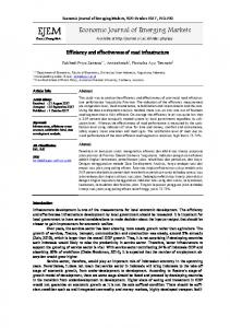
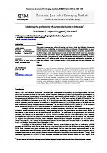
tries, and the national army was around 14,047,124 litre (95.15%), 20,000 litre (0.14%), and 696,093 litre (4.72%) per month, respectively. For diesel, the public group utilized approximately 10,500,086 litre (58.37%); the State-Owned Electricity Company spent about 5,008,750 litre (27.85%); and industries used up around 1,131,699 litre (6.29%). In addition, diesel was also used by the national army with an average of 1,346,996 litres (7.49%) per month. For kerosene, the public group used on average 12,407,917 litre (99.62%), and the national army consumed 46,942 litre (0.38%) monthly. The data of oil consumption in Aceh based on oil type is listed in Figure 1 In line with the growth of oil consumption in Aceh, the population also increased, except for year 2005 the population in Aceh decrease because the Tsunami disaster in the late of December 2004. Similarly, the income per capita grew and there was also change in economic growth in Aceh. The development was followed by a huge number of energy consumption to accommodate it. Generally, energy that is used in the development process consists of three main sectors; transportation, industry, and household sectors. Almost all economic sectors used oil as the main energy to run, even though the industry and household slowly try to use the alternative energy such as electricity. Moreover Indonesia is one of many countries that consume larger energy per unit GDP. Compared to Japan, as a big industrial country, Indonesia was almost twice as higher as Japan in consuming energy. Perhaps, this condition was stimulated by inefficiency of energy consumption. Figure 2 shows the trend Gross Regional Domestic Product (GRDP) in Aceh from 1985 to 2008. It is noted that, GRDP which is used in this case is obtained from two sectors out of nine sectors that contribute for total GRDP since those two sectors have high possibility in using oil in their activities. Those sectors are, first, electricity and water supply, and second, transportation and communication.

40

Avtur

Gasoline

Kerosene

2008

2007

2006

2005

2004

2003

2002

2001

2000

1999

1998

1997

1996

1995

1994

1993

1992

1991

1990

1989

1988

1987

1985

450000 400000 350000 300000 250000 200000 150000 100000 50000 0

1986

!

Diesel

Source: Statistics Aceh (calculated)

3000000 2500000 2000000 1500000 1000000 500000 0

1985 1986 1987 1988 1989 1990 1991 1992 1993 1994 1995 1996 1997 1998 1999 2000 2001 2002 2003 2004 2005 2006 2007 2008

million IDR

Figure 1: Oil consumption in Aceh based on Oil Type Year 1985 – 2008 (in Kilo litters).

Year

Figure 2: Real GRDP of Electricity and Water Supply, and Transportation and CommuniCommun cation Sector in Aceh 1985-2008

There is the same trend between the growths of GRDP (Figure 2) and oil consumption (Figure 1)) in Aceh. Aceh Oil consumption and the gross regional domestic prodpro uct in Aceh have similar upward trend overall. Therefore, this study is necessary to address the effect of oil consumption on economic growth with the main purpose to examine the actual relationship between oil consumption and economic growth in Aceh. Particularly this study investigates the effect of oil consumption on economic growth of Aceh in long run and short run. The he relationship between energy consumption and economic growth has been a well-studied studied topic over the past three decades. Discussion about energy as a natural resource and it’s relationship on economy, Randall (1987) depicted that the growth in consumption (for each of the catca

egories of raw materials) has outstripped the growth in population in U.S. For food and structural materials, material the per-capita growth has been fairly modest, whereas for energy consumption increased increase spectacularly. Additionally, most of the energy curcu rently used comes mes from mineral sources as many as of the structural materials. Food and structural materials aterials came ca from farms and nd forests. Although farm and forest rer sources are renewable, their production has become heavily dependent on minerals for fuel, fertilizer, and pesticides. For the minmi erals, especially fossil fuel, there is theorettheore ically some fixed initial stock (exhaustible stock resources),, that is, the totality of all that nature has provided. Reserves, howevhowe er, are different. The nature of reserves is dynamic. The reserve changes over time depending on prices, technology, and exe


ploration effort. Randall (1987) emphasized that fossil fuels have contributed significantly to economic progress for more than two hundred years (in the case of coal). Oil and natural gas have been used in significant quantities only in the last one hundred years. In this relativel shorter period, however, fossil fuels have made a massive contribution to significant economic growth and standards of living. Some have argued that the high rates of economic growth permitted by the heavy use of fossil fuels have accelerated the formation of capital. During 1930s – the mid-1970s in U.S. encouraged high rates of current use of fossil fuel in activities that seem more nearly related to consumption than to capitalforming investment. In formulating the link between energy consumption and economic growth, this study relies on several thought that could be considered. The classical economists who stressed on technological progress and the importance of capital to productivity were conceptualizing the aggregate production function as the first phase of the Industrial Revolution in England as taking the form: Y = f (D,K,L)

Where Land (D) was referred broadly to include soil and mineral resource (and thus was synonym for “natural resources” as natural resources were understood at the time). Land was thought to be not only important but also fundamentally limited. K and L are capital and labor, respectively (Randall, 1987). By the time the Industrial Revolution continued, capital in production was getting more important and and substituting mineral raw materials for animal and vegetable materials. As technological continued, it became built into expectations and institutional framework. Standards of living were improving, and for the first time industrialization had made the common people in industrial societies better off. Land, broadly defined as natural resources,

41

seemed less of a constraint. Perhaps more important, land itself responded into investment, and so there seemed nothing special or unique about land. The neoclassical aggregate production function was usually expressed as: Y = g(K,L)

In the Contemporary “Human Capital” Perspective, the modern economist, T. W. Schultz assumed that land no longer has any unique significance and is responsive to investment; that is investment in developing “human capital” to increase skills (Farmer, 1997). Thus, the “Schultzian” production function in its most aggregate form as: Y= h(K)

In this formulation, K is given a modern interpretation. Capital in seen as whatever is created by the act of investment and thus include physical plant, educated human minds and bodies, farms and forest that respond to investment and management, and the technologies embodied in all of these productive facilities. Natural resource limitations, according to this viewpoint, are simply not fundamental. They can be overcome by substituting capital (physical and human) and the technology innovations the capital generates and embodies for limited natural resources. Some studies investigated the relationship between growth and natural resources, particularly energy consumption, and some included the passage of time (long-run and short-run relationship) in their studies. Fatai, et al (2004) concluded that a number of industrialized and developing countries agreed to the terms of the Kyoto protocol to conserve energy and reduce emissions. The close relationship between energy consumption and real GDP growth suggests that energy conservation policies are likely to affect real GDP growth. In this paper, the possible impact of energy conservation policies on the New Zealand econo-

42

my was examined and compared with Australia and several Asian economies. Energy consumption and GDP in New Zealand was investigated as well as the causal relationship between GDP and various disaggregate energy data (coal, natural gas, electricity and oil). Based on the energy data used, it appeared that energy conservation policies may not have significant impacts on real GDP growth in industrialized countries such as New Zealand and Australia compared to some Asian economies. Furthermore, the studies have used a multivariate co-integration test to investigate the relationship between economic growth and energy consumption (e.g., Stern, 1993, 2000; Ghali and El-Sakka, 2004). The multivariate methodology is important because of the ongoing change in energy use was countered by the substitution of some factors of production. The results often lead to an insignificant comprehensive impact on local output (Stern, 2000). Yu and Jin (1992) employed co-integration tests to analyze the long-run equilibrium with the level of energy consumption and employment for the case of U.S. They found no evidence of a cointegrating relationship between energy use and either employment or the index of industrial production. This implies that energy consumption is neutral with respect to income and employment over the long run. Masih and Masih (1996) used co-integration analysis of Engle-Granger’s version to study this relationship in a group of six Asian economies. Significant co-integration was found between energy consumption and economic growth in India, Pakistan, and Indonesia, but no co-integration in Malaysia, Singapore, and the Philippines. Stern (2000) extended the previous analysis of Stern (1993) for the post-war period on the U.S. economy by introducing a multivariate co-integration relationship between energy and GDP. The conclusions obtain again that an energy input usage did not seem to be Granger cause GDP. Nevertheless, using a quality-weighted index of

!

energy input was found to be Granger cause GDP. The co-integration tests for both the single static co-integration analysis and the multivariate dynamic co-integration analysis showed that energy was a definitive factor to explain GDP in the U.S. This outcome contradicts to the bivariate model of Yu and Jin (1992), while it supports the conclusions of Stern (1993) that energy was a limited factor in economic growth. Ghali and El-Sakka (2004) used the Johansen co-integration technique to analyze the relationship for output, capital, labor, and energy use in Canada, based on neo-classical one-sector aggregate production technology. The long-run movements of output, capital, labor, and energy consumption was significantly co-integrated. Therefore, energy was not neutral to economic growth. Aktas and Yilmaz (2008) performed ECM to examine the short run and long run causality between oil consumption and economic growth in Turkey during 1970 – 2004. They found that oil consumption has significant impact to economic growth in Turkey both in the short run and the long run. Furthermore, Zaman, Farooq, and Ullah (2011) employed ECM to determine the impact of oil consumption to economic growth in Pakistan for the time period 1972-2008. They found that major sectors of oil consumption (transportation, power generation and industry) were positively contributing on economic growth.

Methods

This study examines the impact of oil consumption on economic growth in Aceh Province during the time period before world commodity prices fall 1985-2008. Type of oil consumption which is examined in this study consists of Avtur, Gasoline, Kerosene, and Diesel oil. All these type of oil will be evaluated to find out their relationship with Aceh’s Gross Regional Domestic Product (GRDP). This study is conducted with secondary data from Statistical Centre Bureau (BPS) Aceh.


Oil consumption data is a proxy of amount of oil supply in Aceh region by PERTAMINA Marketing Unit I Banda Aceh. GRDP data is taken from two industrial origins i.e. electricity and water supply, and transportation and communicationIt doesn’t need to take all total GRDP Aceh from nine industrial origins since the other seven industrial origins are not really have strong relationship with oil usage. The model for this study based on the classical growth theory model. It states that its relationship is positive. Generally, it can be formulated as follows: Y = f (D,K,L), or GRDP = f(AVTR, GSLN, KRSN, DISL) (1) where Land (D) was referred broadly to “natural resources” in the form of oil consumption. K (capital) and L (labor) are constant. Then from the first model above, it is transformed into econometric model form as follows: GRDP = X0 + X1AVTR + X2GSLN + X3KRSN + X4DISL (2) Where GRDP refers to Gross Regional Domestic Product (million IDR), AVTRrefers to Avtur, GSLN refers to Gasoline, KRSN refers to Kerosene, DISL refers to Oil Diesel. Then, X0 refers to Intercept, and X1, X2, X3, X4 refers to parameter.

Stationarity test Unit root test is a test of stationary of the time series data. Considers the AR(1) model: Where yt refers to variable data given, i.e GRDP, AVTR , GSLN , KRSN , and DISL and ut refers to white noise error terms. Subtract from both side of equation (1) to obtain: which can be alternatively written as:

43

where = ( − 1) and is the firstdifference operator. Since under the null hypothesis that = 0 (i.e., = 1), the t value of the estimated coefficient of yt−1 does not follow the t distribution even in large samples; explicitly, it does not have an asymptotic normal distribution. Thus, Dickey and Fuller have shown that under the null hypothesis that = 0, the estimated t value of the coefficient of yt−1 in (3) follows the (tau) statistic estimated in three different forms under three different null hypotheses. In all cases the test concerns whether = 0 so that if DF statistical value is smaller in absolute terms than the critical value then we reject the null hypothesis of a unit root and conclude that yt is as stationary process. As the error term is unlikely to be white noise, Dickey and Fuller extended their test procedure suggesting an augmented version of the test (ADF calculated) which includes extra lagged terms of the dependent variable determined by the Akaike Information Criterion (AIC) or Schwartz Bayesian Critetion (SBC) in order to eliminate autocorrelation. The three forms of the ADF test are given as follows:

If the value of ADF calculated > value of ADF table, so data for variable yt (3) is stationary at degree 0, yt I(0).

Co- integration test

Mostly in time series data analysis our concern is to investigate the long run dynamics relationship among the variables. Two nonstationary time series are said to(4)be cointegrated if their linear combination is stationary. The stationary linear combination (5) and is called the co-integrating equation

44

!

may be interpreted as a long-run equilibrium relationship among the variables. Co-integration between two series also implies a particular kind of model, called an Error Correction Model (ECM), for the short-term dynamics. A linear combination of GRDPt , AVTRt , GSLNt, KRSNt, and DISLt can be directly formulated as: GRDPt = 0 + 1AVTRt + 2GSLNt + (9) 3KRSNt + 4DISLt + ut

Let us write this as: ut= GRDPt - 0 -

1AVTRt 3KRSNt - 4DISLt

2GSLNt -

(10) Suppose that now subject ut to unit root analysis and find that it is stationary; that is, it is I(0). This is an interesting situation, for although GRDPt ,AVTRt , GSLNt , KRSNt ,DISLt are individually I(n), that is, their linear combination (9) is I(0). In this case it is said that the variables are cointegrated. Economically speaking, variables will be co-integrated if they have a long-term, or equilibrium, relationship between them. In short, provided we check that the residuals from regressions like (10) are I(0) or stationary, the traditional regression methodology (including the t and F tests) that we have considered extensively is applicable to data involving (non-stationary) time series. The valuable contribution of the concepts of unit root, co-integration, etc. is to force us to find out if the regression residuals are stationary. As Granger notes, “A test for cointegration can be thought of as a pre-test to avoid ‘spurious regression’ situations.” In the language of co-integration theory, a regression such as (9) is known as a co-integrating regression and the slope parameter 1, 2, 3, 4 are known as the cointegrating parameter. The concept of cointegration can be extended to a regression model containing k regressors. In order to know whether the regression has co-integrated or not, it should be performed the stationary test of the residual

or error term of the long run equation. First regress the equation (2) with Ordinary Least Square method that yields the residual ut. The next step is performing stationary test for the residual. The stationary test method is the same as stationary test for unit root. If the residual of the equation is stationary at level 0 or I(0), it means the variables co-integrated.

ECM estimation

The existence of co-integration relationships indicates that there are long-run relationships among the variables, and thereby Granger causality among them in at least one direction. The ECM was introduced for correcting disequilibrium and testing for long run and short run causality among cointegrated variables. Derive from the equation (2) with GRDP as the dependent variable and AVTR, GSLN, KRSN, DISL as the independent variable. The real economic system are rarely in equilibrium, so when dependent variable takes a value different from its equilibrium value, the different between the dependent variable and the independent variable is GRDP - X0 + X1AVTR + X2GSLN + X3KRSN + X4DISL. This quantity is known as disequilibrium error (Thomas, 1996). Since between dependent and independent variable as noted above rarely in equilibrium, what the applied econometrician usually observes is a short run or disequilibrium relationship involving lagged values of variables of GRDP, AVTR, GSLN, KRSN, and DISL. Suppose this take the form: GRDPt = b0 + b1AVTRt + b2AVTRt-1 + b3GSLNt + b4GSLNt-1 + b5KRSNt + b6KRSNt-1 + b7DISLt + b8DISLt-1 + GRDPt-1 + t , 0 < < 1 (11) Subtracting GRDPt-1 from each side yields: GRDPt - GRDPt-1 = b0 + b1AVTRt + b2AVTRt-1 + b3GSLNt + b4GSLNt-1 + b5KRSNt + b6KRSNt-1 + b7DISLt + b8DISLt-1 - (1- ) GRDPt-1 + t (12)


Subtracting and adding b1AVTRt-1, b3GSLNt-1, b5KRSNt-1, and b7DISLt-1 from the right hand side of (12) yields:

GRDPt = b0 + b1 AVTRt + (b1+b2)AVTRt-1 + b3 GSLNt + (b3+b4)GSLNt-1 + b5 KRSNt + (b5+b6)KRSNt-1 + b7 DISLt + (b7+b8)DISLt-1 - GRDPt-1 + t (13)

Where = 1 – . Then reparameterize (13) as follows:

GRDPt = b0 + b1 AVTRt + b3 GSLNt + b5 KRSNt + b7 DISLt - (GRDPt-1 1AVTRt-1 - 2GSLNt-1 - 3KRSNt-1 (14) 4DISLt-1) + t Where there are some new parameter: 1 = (b1+b2)/ , 2 = (b3+b4)/ , 3 = (b5+b6)/ , 4=(b7+b8)/ . Since GRDPt-1 - 1AVTRt-1 2GSLNt-1 - 3KRSNt-1 - 4DISLt-1 is called

Error Correction Term, so the equation (14) could be written as:

GRDPt = b0 + b1 AVTRt + b3 GSLNt + b5 KRSNt + b7 DISLt - ECT + t (15)

Meanwhile, to know the effect of independent variable to dependent variable for long run in equation (15), it should find out the coefficient variable consisting of C = b0 / , AVTR = (b1 + ) / , GSLN = (b3 + ) / , KRSN = (b5 + ) / , DISL = (b7 + ) / . Finally, the definitions and scope of the variables involved in this study are: GRDPt and GRDPt-1 are Gross Regional Domestic Product in Aceh at time t and t-1, respectively and GRDPt is the change of Gross Regional Domestic Product in Aceh at time t (in million IDR or Indonesian Rupiah). Meanwhile, AVTRt and AVTRt-1 (Avtur), GSLNt and GSLNt-1 (Gasoline), KRSNt and KRSNt-1 (Kerosene), DISLt and DISLt-1 (oil diesel) are oil types of energy consumed at time t and time t-1 in kilo liter (kL). AVTRt, GSLNt, KRSNt, DISLt are the changes of Avtur, Gasoline, Kerosene, and Diesel at time t in kilo Liter (kL). Furthermore, 0 and b0 are the intercept; 1, 2, 3, 4 and b1, b2, b3, b4, b5, b6, b7, b8, , are the variable parameters; utand t are error term at time t; and ECT is the error correction term.

45

Result and Discussion

Unit root test is done in correlation with stationary test. Based on the stationary test, it is known that all time series data Gross Regional Domestic Product (GRDP), Oil consumption such as Avtur (AVTR), Gasoline (GSLN), Kerosene (KRSN), and Diesel (DISL) are not stationary at level or I(0) since the value of ADF calculated is less than ADF table (Mac Kinnon critical values 5%). According to the result of unit root test above, all variables are not stationary in level, so it needs to carry out integration degree test. The result of integration degree test show that the ADF calculated value is more than ADF tabel or Mac Kinnon critical values at 5% for each variable GRDP, AVTR, GSLN, KRSN, and DISL. So all are stationary at degree 1 or I(1). Co-integration test is performed by checking the error term or residual stationary level from the long run equation. If the residual is stationary at level or I(0) it means the dependent variable and the independent variables are co-integrated. The long run equation is given as (9): GRDPt = 0 + 1AVTRt 4DISLt + ut.

+

2GSLNt

+

3KRSNt

+

Regressing equation (9) by Ordinary Least Square (OLS) method and it will be obtained the residual ut. The test shown that ADF calculated value of ut. is higher than critical values 5%. ADF calculated is 5.0984 meanwhile the critical value for 5% level is 2.9981. Thus it states that the residual of the long run equation is stationary at level or I(0), which means the variables are co-integrated. ECM is used to evaluate the impact of AVTR, GSLN, KRSN, and DISL to GRDP in short run. Refer to equation (15), GRDPt = b0 + b1 AVTRt + b3 GSLNt + b5 KRSNt + b7 DISLt - ECT + t. The

regression result from this ECM equation is shown in Table 1. Table 1 shows that variables AVTR, GSLN, and KRSN are not significant, but

46

!

DISL is significant at confidence level = 10% (one-tailed statistical test). From ECM estimation test, it is obtained that F-statistic is 4.7320 with probability value equal to 0.0068 that less than = 1%. It means that overall independent variables significantly simultaneously affect dependent variable. Also from ECM estimation test, it is obtained R2 = 0.5819 which indicates the variation of independent variables of the model can explain the variation of dependent variable by 58.19%. The rest 41.81 % is explained by confounding variables that are not included in the equation. GRDP, AVTR, GSLN, KRSN and DISL have long run relationship since they are co-integrated, whereas the residual ut from the long run equation is stationary at level with t-statistic -5.098431 and probability 0.0005. ECM model could explain dynamic behavior of the equation in short run and long run. In short run, coefficient value of Avtur is 28.2026 which is not significant statistically. It explains that Avtur change is not affecting economic growth in short run. The coefficient value of Gasoline is – 0.4335 which is not significant. It implies that Gasoline change is not affecting economic growth. Kerosene change is not also significant statistically. Its coefficient value is –

4.2885. The t-statistic value is - 1.6137 less than t-table critical value -1.740 (absolute value). Also the probability for this variable is 0.1250 that conclude Kerosene change do not significantly influence GRDP change. It implies that Gasoline change is not affecting economic growth. The coefficient value of Diesel change is 3.4803. Oil consumption has t-statistic value 1.9245 which is higher than t-table critical value 1.740. It means, this variable is significant statistically. Also the probability for this variable is 0.0712 that conclude Diesel change significantly influence GRDP change in level of significant 5%. In the other word, Diesel change is affecting economic growth in the short run. Error Correction Term value that is equal to adjustment speed toward long run equilibrium shows coefficient value 0.8469 with t-statistic -2.5768. This t-statistic value is higher than t-table critical value -1.740. Thus, Error Correction Term is significant statistically. The probability value is 0.0196 that means significant in level of significant 5%. Coefficient of adjustment is 0.8469, which means around 84.69% disequilibrium economic growths between actual and expectation will be eliminated in one year.

Table 1: Error Correction Model Estimation Dependent Variable: GRDP Variable

Coefficient 28.2026 - 0.4335 - 4.2884 3.4803 0.8469 50350.89

AVTR GSLN KRSN DISL ECT C Source: Estimation

Variable C AVTR GSLN KRSN DISL

Formula

b0 / (b1 + ) / (b3 + ) / (b5 + ) / (b7 + ) /

t-statistic 0.9327 - 0.2179 - 1.6041 2.5093 3.9986 1.0794

Table 2: Long Run Effect Coefficient Result 59453.17 33.3010 0.4881 -4.0636 5.1095

t-statistic 1.0954 0.9398 -0.2112 -1.6137 1.9245

Probability 0.3640 0.8301 0.1271 0.0225 0.0009 0.2955

Std. Error 45967.36 30.0092 2.0529 2.6576 1.8085


In the long run, the coefficient value for Avtur is 33.3010, but Avtur is not affect GRDP since statistically t-statistic value 0.9398 is less than t-table critical value 1.740. So do Gasoline, with coefficient value 0.4881, it is not significant statistically influencing GRDP since the t-statistic value -0.2112 is less than t-table critical value -1.740. The same thing occurred to Kerosene that has coefficient value 4.0636. The t-statistic value -1.6137 is less than t-table critical value 1.740 which means it is not affecting GRDP in long run. For Diesel, as shown on Table 10, it is significant statistically. Coefficient value for Diesel is 5.1095 and t-statistical value 1.9245 that is higher than t-table critical value 1.740. It explains that, for long run, Diesel affect positively and significantly Gross Domestic Regional Product or economic growth. So, for long run if Diesel consumption increase 1 kilo Litre, it will increase GRDP 5.109 million IDR, and vice versa for long run, if Diesel consumption decrease 1 kilo Litre result in GRDP decrease around 5.109 million IDR, ceteris paribus, (Table 2). In general, there is a long run relationship between oil consumption and economic growth in Aceh. In the long run, oil consumption of Diesel impact positively the real GRDP in 1985-2008 year period that means increasing oil consumption of Diesel in Aceh increased economic growth in Aceh. Meanwhile oil consumption of Avtur, Gasoline, and Kerosene do not affect real GRDP in Aceh. This result is in line with the real condition since oil consumption could not be detached from economic activities. Market activities like distribution of goods or shipment and all of services need transportation to support the work and hence, of course diesel oil plays a significant role on that process. The same illustration take place in business activities and services which could not detached from electricity. To generate electricity, in Aceh, until now it is still depend on oil

47

power generator which use diesel, thus diesel oil is still need in business activities and services even though that is a non directly usage since it has been transformed into electricity energy. In the short run, as per ECM result, Diesel oil consumption change impacts economic growth in Aceh. Diesel oil consumption variable impacts significantly and positively for real GRDP change in Aceh. This phenomenon might be occurred in correlation with the usage of diesel oil for transportation. Diesel Oil consumption is increasing along with the automobiles sales increase. The demand of diesel cars increase every year in Aceh, followed by the increase of diesel oil consumption demand automatically. Increasing mobility of residence in Aceh region that use public transportation like minibus and bus will also influence diesel oil consumption since those transportation mode use diesel oil for the energy. More people traveling with minibus or bus use more diesel. For this point of view oil consumption in transportation sector has directly pushed the economy in Aceh. Meanwhile oil consumption change for Avtur, Gasoline, and Kerosene, in the short run, do not impact real GRDP in Aceh. In relation to the result of this study that diesel oil consumption has significant impact to the economic growth in Aceh, therefore the interest parties involve in production and distribution of oil, like PERTAMINA and the Government should ensure the oil stock is sufficient enough to be delivered and also Government and society should supervise well the oil distribution so that it could be consumed optimally.

Conclusion

There are some important points of this study consisting of (1) diesel oil consumption has a significant positive impact to economic growth in Aceh, both the long run and the short run. However, Avtur, Gasoline, and Kerosene oil consumption do

48

!

not; (2) In long run, increase 1 kilo Litre Diesel oil consumption will increase 5.109 million IDR real GRDP in Aceh, and vice versa decrease 1 kilo Litre Diesel oil onsumption will decrease 5.109 million IDR real GRDP in Aceh; (3) In short run, 1 kilo Litre change Diesel oil consumption will change around 3.483 million IDR real GRDP in Aceh; and (4) The Error Correction Term (ECT) in this model shows that the model is convergence towards the equilibrium with value 0.8469. Therefore, all interest parties that in line with energy sector especially oil should pay attention to ensure the oil consumption especially type Diesel in Aceh run well since it has a significant impact to the real GRDP or economic growth in Aceh. They have to guarantee that the distribution of the oil run smoothly. Furthermore, the findings of this study can be used as starting points for much more focused efforts. It will suggest for the further study to incorporate other variables which have indirect and direct effects on economic growth. Then, it can capture the actual condition of economic activities completely, particularly economic growth of Aceh related to oil consumption.

References

Aktas, C. and V. Yilmaz (2008), “Causal Relationship between Oil Consumption and Economic Growth in Turkey,” Kocaeli niversitesi Sosyal Bilimler Enstit Dergisi, 15(1), 45-55. Asteriou, D. and S.G. Hall (2007), Applied Econometrics A Modern Approach Revised Edition, Palgrave Macmillan. British Petroleum (2011), BP Statistical Review of World Energy June, 2011, British Petroleum Farmer, R.E.A. (1997), Macroeconomics,

Department of Economics UCLA, 405 Hilgard Avenue, Los Angeles CA 90024.

Fatai, K, L. Oxley and F.G. Scrimgeour (2004), “Modelling the Causal Relationship between Energy Consumption and GDP in New Zealand, Australia, India, Indonesia, The Philippines and Thailand,” Mathematics and Computers in Simulation 64(3-4), 431–445.

Ghali, K.H., M.I.T. El-Sakka (2004), “Energy Use and Output Growth in Canada: a Multivariate Cointegration Analysis, “ Energy Economics, 26(2), 225-238. Energy Information Administration (2004), International Energy Outlook 2004, Energy Information Administration, Washington DC. Masih, A.M.M., Masih, R., (1996), “Energy Consumption, Real Income and Temporal Causality: Results from a Multi-country Study based on Cointegration and Error-Correction Modelling Techniques,” Energy Economics, 18(3), 165-183. Randall, A. (1987), Resource Economics

Second Edition; An Economic Approach to Natural Resource and Environmental Policy, John Wi-

ley&Sons, Inc. USA. Stern, D.I. (1993), “Energy and Economic Growth in the USA, a Multivariate Approach,” Energy Economics 15(2), 137–150. Stern, D.I. (2000), “A Multivariate Cointegration Analysis of the Role of Energy in the US Economy,” Energy Economics 22(2), 267–283. Stern, D.I. and C.J. Cleveland (2004), “Energy and Economic Growth,” Working Paper No. 0410, Rensselaer Polytechnic Institute, New York. Syahnur, S. (2009). The Impact of Price Change on the Poor in Nanggroe Aceh Darussalam Province, Indo-


nesia; A Case Study on Oil Price”,

Cuvillier Verlag Gottingen, Germany, August. Yu, E.S.H. and J.C. Jin (1992), Cointegration Tests of Energy Consumption, Income, and Employment,” Resources Energy, 14(3), 259-266.

49

Zaman, B., M. Farooq and S. Ullah (2011), “Sectoral Oil Consumption and Economic Growth in Pakistan: An ECM Approach,” American Journal

of Scientific and Industrial Research, 2(2), 149-156.