Educational Data Mining - Semantic Scholar

Workshop of Educational Data Mining

Educational Data Mining

Cecily Heiner (Co-chair) Neil Heffernan (Co-chair) Tiffany Barnes (Co-chair)

Supplementary Proceedings of the 13th International Conference of Artificial Intelligence in Education. Marina del Rey, CA. USA. July 2007


Educational Data Mining Workshop (http://www.educationaldatamining.org/) Cecily Heiner; University of Utah; [email protected] (Co-chair) Neil Heffernan; Worcester Polytechnic Institute; [email protected] (Co-chair) Tiffany Barnes; University of North Carolina at Charlotte, [email protected] (Co-chair)

Introduction Educational data mining is the process of converting raw data from educational systems to useful information that can be used to inform design decisions and answer research questions. Data mining encompasses a wide range of research techniques that includes more traditional options such as database queries and simple automatic logging as well as more recent developments in machine learning and language technology. Educational data mining techniques are now being used in ITS and AIED research worldwide. For example, researchers have used educational data mining to: o Detect affect and disengagement o Detect attempts to circumvent learning called "gaming the system" o Guide student learning efforts o Develop or refine student models o Measure the effect of individual interventions o Improved teaching support o Predict student performance and behavior However, these techniques could achieve greater use and bring wider benefits to the ITS and AIED communities. We need to develop standard data formats, so that researchers can more easily share data and conduct meta-analysis across tutoring systems, and we need to determine which data mining techniques are most appropriate for the specific features of educational data, and how these techniques can be used on a wide scale. The workshop will provide a forum to present preliminary but promising results that can advance our knowledge of how to appropriately conduct educational data mining and extend the field in new directions. Topics They include, but are not limited to: o What new discoveries does data mining enable? o What techniques are especially useful for data mining? o How can we integrate data mining and existing educational theories? o How can data mining improve teacher support? o How can data mining build better student models? o How can data mining dynamically alter instruction more effectively? o How can data mining improve systems and interventions evaluations? o How do these evaluations lead to system and intervention improvements? o How is data mining fundamentally different from other research methods?


TABLE OF CONTENTS Evaluating problem difficulty rankings using sparse student data………….…………1 Ari Bader-Natal, Jordan Pollack Toward the extraction of production rules for solving logic proofs…………………...11 Tiffany Barnes, John Stamper Difficulties in inferring student knowledge from observations (and why you should care)………………………………………………………………………………………...21 Joseph E. Beck What’s in a word? Extending learning factors analysis to modeling reading transfer………………………………………………………………………..…………….31 James M. Leszczenski, Joseph E. Beck Predicting student engagement in intelligent tutoring systems using teacher expert knowledge ……….………………………………………………………………………...40 Nicholas Lloyd, Neil Heffernan, Carolina Ruiz Analyzing fine-grained skill models using Bayesian and mixed effects methods ……………………………………………………………………………………………….50 Zachary Pardos, Mingyu Feng, Neil Heffernan, Cristina Heffernan, Carolina Ruiz Mining learners’ traces from an online collaboration tool……………………………..60 Dilhan Perera, Judy Kay, Kalina Yacef, Irena Koprinska Mining on-line discussions: Assessing technical quality for student scaffolding and classifying messages for participation profiling………………………………………. .70 Sujith Ravi, Jihie Kim, Erin Shaw

All in the (word) family: Using learning decomposition to estimate transfer between skills in a reading tutor that listens………………………………………………..……..80 Xiaonan Zhang, Jack Mostow, Joseph Beck


Evaluating Problem Difficulty Rankings Using Sparse Student Response Data Ari BADER-NATAL 1 , Jordan POLLACK DEMO Lab, Brandeis University Abstract. Problem difficulty estimates play important roles in a wide variety of educational systems, including determining the sequence of problems presented to students and the interpretation of the resulting responses. The accuracy of these metrics are therefore important, as they can determine the relevance of an educational experience. For systems that record large quantities of raw data, these observations can be used to test the predictive accuracy of an existing difficulty metric. In this paper, we examine how well one rigorously developed – but potentially outdated – difficulty scale for American-English spelling fits the data collected from seventeen thousand students using our SpellBEE peer-tutoring system. We then attempt to construct alternate metrics that use collected data to achieve a better fit. The domain-independent techniques presented here are applicable when the matrix of available student-response data is sparsely populated or non-randomly sampled. We find that while the original metric fits the data relatively well, the datadriven metrics provide approximately 10% improvement in predictive accuracy. Using these techniques, a difficulty metric can be periodically or continuously recalibrated to ensure the relevance of the educational experience for the student.

1. Introduction Estimates of student proficiency and problem difficulty play central roles in Item Response Theory (IRT) [11]. Several current educational systems make use of this theory, including our own BEEweb peer-tutoring activities [2,8,9,13]. IRT-based analysis often focuses on estimating student proficiency in the task domain, but the challenge of estimating problem difficulty should not be overlooked. While student proficiency estimates can inform assessment, problem difficulty estimates can be used to refine instruction: these metrics can affect the selection and ordering of problems posed and can influence the interpretation of the resulting responses [6]. It is therefore important to choose a good difficulty metric initially and to periodically evaluate the accuracy of a chosen metric with respect to available student data. In this paper, we examine how accurately one rigorously developed – but potentially outdated – difficulty scale for the domain of American-English spelling predicts the data collected from students using our SpellBEE system [1]. The defining challenge in providing this assessment lies in the nature of the data. As SpellBEE is a peer-tutoring system, the challenges posed to students are determined by other students, resulting in data that is neither random nor complete. In this 1 Correspondence to: Ari Bader-Natal, Brandeis University, Computer Science Department – MS 018. Waltham, MA 02454. USA. Tel.: +1 781 736 3366; Fax: +1 781 736 2741; E-mail: [email protected].

1


work, we rely on a pairwise comparison technique designed to be robust to data with these characteristics. After assessing the relevance of this existing metric (in terms of predictive accuracy), we will examine some related techniques for initially constructing a difficulty metric based on non-random, incomplete samples of observed student data.

2. American-English spelling: A sample task domain The educational system examined here, SpellBEE, was designed to address the task domain of American-English spelling [1]. SpellBEE is the oldest of a growing suite of web-based reciprocal tutoring systems using the Teacher’s Dilemma as a motivational mechanism [2]. For the purposes of this paper, however, the mechanisms for motivation and interaction can be ignored, and the SpellBEE system and the difficulty metric used by it can be specifically re-characterized for an educational data mining audience. 2.1. Relevant characteristics of the SpellBEE system Students access SpellBEE online at SpellBEE.org from their homes or schools. As of May 2007, over 17,000 students have actively participated. After creating a user account, a student is able to log in, choose a partner, and begin the activity.2 During the activity, students take turns posing and solving spelling problems. When posing a problem, the student selects from a short list of words randomly drawn from the database of wordchallenges. This database is comprised of 3,129 words drawn from Greene’s New Iowa Spelling Scale (NISS), which will be discussed in the next section [12].3 When responding to a problem, the student types in what they believe to be the correct spelling of the challenge word. The accuracy of the response is assessed to be either correct or incorrect. Figure 1 presents a list of the relevant data stored in the SpellBEE server logs. To date, we have observed over 64,000 unique (case-insensitive) responses to the challenges posed,4 distributed across over 22,000 completed games consisting of seven questions attempted per student. Student participation, measured in games completed, has not been uniform, however. Of the challenges in the space, most students have only attempted a very small fraction. In fact, when examining the response matrix of every student by every challenge, less than 1% of the matrix data is known. An important characteristic of the SpellBEE data, then, is that the response matrix is remarkably sparse. Given that the students acting as tutors are able to – and systemically motivated to – express their preferences and hunches through the problems that they select, another important characteristic of the SpellBEE data is that the data present in the studentchallenge response matrix is also biased. The effects of this bias can be found in the following example: 16% of student attempts to spell the word “file” were correct, while 66% of attempts to spell the word “official” were correct. The average grade level among the first set of students was 3.9, while for the second set it was 6.4. In Section 3.2 we 2 In the newer BEEweb activities, if no one else is present, a student can practice alone on problems randomly drawn from the database of challenges posed in the past. 3 In SpellBEE, the word-challenges are presented in the context of a sentence, and so of the words in Greene’s list, we only use those found in the seven public-domain books that we parsed for sentences. 4 Of these, 17,391 were observed more than once. In this paper, we restrict the set of responses that we consider to this subset. See Footnote 7 for the rationale behind this.

2


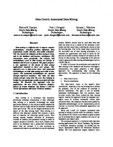
Figure 1. The SpellBEE server logs data about each turn taken by each student, as shown in the first list. The data in the first list is sufficient to generate the data included in the second list.

1. 2. 3. 4. 5. 6.

time : a time-stamp allows responses to be ordered game : identifies the game in which this turn occurred tutor : identifies the student acting as the tutor in this turn tutee : identifies the student acting as the tutee in this turn challenge : identifies the challenge posed by the tutor response : identifies the response offered by the tutee

1. difficulty : the difficulty rating of the challenge posed by the tutor 2. accuracy : the accuracy rating of the response offered by the tutee will present techniques designed to draw more meaningful difficulty information from this type of data. 2.2. Origin, use, and application of the problem difficulty metric When trying to define a measure of problem difficulty for the well-studied domain of American-English spelling, we were able to benefit from earlier research in the field. Greene’s “New Iowa Spelling Scale” provides a rich source of data on word spelling difficulty, drawn from a vast study published in 1954. Greene first developed a methodology for selecting words for his list (5,507 were eventually used.) Approximately 230,000 students from 8,800 classrooms (grades 2 through 8) around the United States participated in the study, totally over 23 million spelling responses [12]. From these, Greene calculated the percentage of correct responses for each word for each grade. This table of success rates is used in SpellBEE to calculate the difficulty of each spelling problem for students, whose grade level is known.

3. Techniques for assessing relative challenge difficulty The research questions addressed in this paper focus on the fit of the difficulty model based on the NISS data to the observed SpellBEE student data. Two different techniques are involved in the calculating this fit. The first converts the graded NISS data to a linear scale. The second identifies from the observed student data a difficulty ordering over pairs of problems, in a manner appropriate for a sparse and biased data matrix. Both will be employed to address the research questions in the following sections. 3.1. Linearly ordering challenges using the difficulty metric Many subsequent studies have explored various aspects of Greene’s study and the data that it produced. Cahen, Craun, and Johnson [5] and, later, Wilson and Bock [14] explore the degree to which various combinations of domain-specific predictors could account for Greene’s data. Initially starting with 20 predictors, Wilson and Bock work down to a regression model with an adjusted R2 value of 0.854.5 Here, we not interested in 5 The

most influential of which being the length of the word.

3


Figure 2. Difficulty data for two words from the NISS study are plotted, and the I50 statistics are calculated.

I50("acknowledge")=7.875

"above" "acknowledge"

50 % I50("above")=3.7

Percentage of students with correct responses

100 %

0% 2

3

4 5 6 Student grade level

7

8

predicting the NISS results, but instead are interested in assessing the fit (or predictive power) of the 1954 NISS results to observations made of students using SpellBEE over 50 years later. We will drawn upon one statistic used by Wilson and Bock: the onedimensional flattening of the seven-graded NISS data. This statistic, which they refer to as the “location” of the word, is the (fractional) grade level at which 50% of the NISS students correctly spell word w.6 We denote this as I50 (w). Figure 2 illustrates how the graded difficulty data that is used to derive this statistic for two different words. The value of this statistic is that it provides a single grade-independent difficulty value for a word that can be compared directly to that of other words. 3.2. Identifying pairwise difficulty orderings using observed student data Given the characteristics of the data collected from the SpellBEE system, identifying the more difficult of a pair of problems based on this data is not trivial. The percentage of correct responses to a challenge, the calculation used to generate the NISS data, is not appropriate here, as the assignment of challenges to students was done in a biased, nonrandom manner (recall the “file”/“official” example from Section 2.1.) Tutors, in fact, are motivated to base their challenge selection on the response accuracies that they anticipate. A more appropriate measure, rooted in several different literatures, is to assess pairwise problem difficulties on distinctions indirectly indicated by the students. In the statistics literature, McNemar’s test provides a statistic based on this concept [10], in the IRT literature, this is used as a data reduction strategy for Rasch model parameter estimation [7], and the Machine Learning literature includes various approaches to learning 6 Wilson and Bock calculate the 50% threshold based on a logistic model fit to the discrete grade-level data, while we calculate the threshold slightly differently, based on a linear interpolation of the grade-level data.

4


Table 1. While the I50 metric flattens the grade-specific NISS data to a single dimension, the relative difficulty ordering of most word-pairs based on the graded NISS data is the same as when based on the I50 scale. In this table, we quantify the amount of agreement between I50 and each set of grade-specific NISS data using Spearman’s rank correlation coefficient. The strong correlations observed suggest that the unidimensional scale sufficiently captures the relative difficulty information from the original NISS dataset. (The number of words, N, varies by grade, as the NISS study did not show several of the harder words to the younger students.) Grade

N

Spearman’s ρ

2 3 4

2218 3059 3126

0.751 0.933 0.977

5 6 7 8

3129 3129 3129 3129

0.974 0.960 0.935 0.915

rankings based on pairwise preferences [4]. Assume that for some specific pair of problems, such as the spelling of the words “about” and “acknowledge”, we first identify all students in the SpellBEE database who have attempted both words. Given that response accuracy is dichotomous, there are only four possible configurations of a student’s response accuracy to the pair of challenges. In the cases where the student responds to both correctly or incorrectly, no distinction is made between the pair. But in the cases where the student correctly responds to one but incorrectly to the other, we classify this as a distinction indicating a difficulty ordering between the two problems.7 It is also worth stating that in this study, we assume a “static student” model, so we are not concerned with the order of these two responses. At the cost of some data loss, one could instead assume a “learning student” model, for which only a correct response on one problem followed by an incorrect response on the other would define a distinction. Had the incorrect response been observed first, we could not rule out the possibility that the difference was due to a change in the student’s abilities over time, and not necessarily an indication of difference in problem difficulties.8 An example may clarify. If counting the number of both directional distinctions made by all students (e.g. 12 students in SpellBEE spelled “about” correctly and “acknowledge” incorrectly, while 2 students spelled “about” incorrectly and “acknowledge” correctly), we have a strong indication of relative problem difficulty. McNemar’s test assigns a significance to this pair of distinction counts. In this work, we more closely follow the IRT approach, relying only the relative size of the two counts (and not the significance.) Thus, since 12 distinctions were found in one direction and only 2 in the other, we say that we observed the word “about” to be easier than the word “acknowledge” based on collected SpellBEE student data. If distinctions were available for every problem pair, 7 We recognize that some distinctions are spurious, for which the incorrect response was not reflective of the student’s abilities. Here we take a simplistic approach of identifying and ignoring non-responses (in which the student typed nothing) and globally-unique responses (which no other student ever responded, to any challenge.) Globally-unique responses encompass responses from students who don’t yet understand the activity, responses from students who did not hear the audio recording, responses from student attempting to use the response field as a chat interface, and responses from students making no effort to engage in the activity. 8 Another possible model is a “dynamic student” model, for which student abilities may get better or worse over time. Under this model, no distinctions can be definitively attributed to difference in problem difficulty.

5


a total of 3,129 × 3,128 = 9,787,512 pairwise problem orderings could be expressed. In our collected data so far, we have 3,349,602 of these problem pairs for which we have distinctions recorded. In the subsequent sections, we measure the fitness of a predictive model (like I50 ) based on how many of these pairwise orderings are satisfied.9

4. Assessing the fit of the NISS-based I50 model to the SpellBEE student data Given the NISS-based I50 difficulty model of problem difficulty and the data-driven technique for turning observed distinctions recorded in the SpellBEE database into pairwise difficulty orderings, we can now explore various methods to assess the applicability of the model to the data. 4.1. Assessing fit with a regression model The first method is to construct a regression model that uses I50 to predict observed difficulty. Since observed difficulty is currently available only in pairwise form, this requires an additional step in which we flatten these pairwise orderings into one total ordering over all problems. As this is a highly non-trivial step, the results should be interpreted tentatively. Here, we accomplish a flattening by calculating, for each challenge, the percentage of available pairwise orderings for which the given challenge was the more difficult of the pair. So if 100 pairwise orderings involve the challenge word “acknowledge”, and 72 of these found “acknowledge” to be the harder of the pair, we would mark “acknowledge” as harder than 72% of other words. A regression model was then built on this, using I50 as a predictor of the pairwise-derived percentage. The model, after filtering out data points causing ceiling and floor effects (i.e. I50 (w) = 2.0 or I50 (w) = 8.0), had an adjusted R2 value of 0.337 (p < 0.001 for the model). The corresponding scatterplot is shown in Figure 3.10 The relatively low adjusted R2 value is likely at least partially a result of the flattening step (rather than solely due to poor fit.) Had we flattened the data differently, this value would clearly change. In order to obtain a more reliable measure of model fitness, we seek to avoid any unnecessary processing of the mined data. 4.2. Assessing fit with as the percentage of agreements on pairwise difficulties The second method that we explore provides a more direct comparison, without any further flattening of the student data. Here, we simply calculate the percentage of observed pairwise difficulty orderings (across all challenges) for which the I50 model correctly predicts the observed pairwise difficulty ordering. When we do this across all of the 3,349,602 difficulty orderings that we have constructed from the student data, we find that the I50 model correctly predicts 2,534,228 of these pairwise orderings, providing a 75.66% agreement with known pairwise orderings from the mined data. Remarkably, we found that the predictive accuracy of the I50 model did not significantly change as the 9 Note

that it is not be possible to achieve a 100% fit, as some cycles exist among these pairwise orderings.

10 The outliers in this plot mark the problems that are ranked most differently by the two measures. The word

“arithmetic”, for example, was found to be difficult by SpellBEE students, but was not found to be particularly difficult for the students in the NISS study. Variations like this one may reflect changes in the teaching or in the frequency of usage since the NISS study was performed 50 years ago.

6


Figure 3. Words are plotted by their difficulty on the I50 scale and by the percentage of other words for which the observed pairwise orderings found the word to be the harder of the pair. An adjusted R2 value of 0.490 was calculated for this model. (When ignoring the words affected by a ceiling or floor effect in either variable, the adjusted R2 value drops to 0.377.)

Percentage of comparisons finding word harder

100 %

50 %

0% 2

3

4

5 6 I50 Difficulty Value

7

8

quantity of student data used for the distinction varied. 75.1% of predictions based on one distinction were accurate, while 74.7% of predictions based on 25 distinctions were accurate (intermediate values ranged from 71.0% to 77.6%). This flat relationship suggests that pairwise difficulty orderings constructed from a minimal amount of observed data may be just as accurate, in the aggregate, as those orderings constructed when additional data is available.

5. Incorporating SpellBEE student data in a revised difficulty model We now know that there is a 75.66% agreement in pairwise difficulty orderings between the I50 difficulty metric derived from the NISS data and the observed pairwise preferences mined from the SpellBEE database. Can we improve upon this? We will present an approach that iteratively updates the I50 problem difficulty estimates using the mined data and a logistic regression model. Rather than producing a single predictive model, we construct one logistic model for each challenge, and use these fitted model to update our estimates of the problem difficulty. Applied iteratively, we hope to converge on problem difficulty metric that better fits the observed data. This process is inspired by the parameter estimation procedures for Rasch models [11], which may not be directly applicable due to the large size of our problem space. For a given challenge c1 (e.g. “acknowledge”), we can first generate the list of all other challenges for which SpellBEE students have expressed distinctions (in either direction.) In Section 3.2, we chose to censor these distinctions in order to generate a bi-

7


Figure 4. A logistic regression model is used to estimate the difficulty of the word “abandon.” At left, the first estimate is based on the original I50 difficulty values. At right, the third iteration of the estimate is constructed based on data from the previous best estimate. The point estimate dropped from 8.0 (from I50 ) to 7.06 (from iteration 1) to 6.81 (from iteration 3.) 100 % Percentage of distinctions finding word harder

Percentage of distinctions finding word harder

100 %

50 %

0% 2

3

4

5 6 Difficulty Estimate

7

8

50 %

0% 2

3

4

5 6 Difficulty Estimate

7

8

nary value representing the difficulty ordering. Here we will make use of the actual distinction counts in each direction. For each challenge with which pairwise distinctions for c1 are available, we note our current-best estimate of the difficulty of c2 (initially, using I50 values), and note the number of distinctions indicating that c1 is the more difficult challenge. We can then regress the grouped distinction data on the problem difficulty estimate data to construct a logistic model relating the two. For some c1 , if the relationship is statistically significant, we can use it to generate a revised estimate for the difficulty of that challenge. By solving the regression equation for the c2 problem difficulty value for which 50% of distinctions find c1 harder, we can calculate the difficulty of a problem for which relative-difficulty distinctions are equally likely in either direction. This provides a revised estimate for the difficulty of the original problem, c1 . We use this procedure to calculate revised estimates for every challenge in the space (unless the resulting logistic regression model is statistically not significant, in which case we retain our previous difficulty estimate.) This process can be iteratively repeated, using the revised difficulty estimates as the basis of the new regression models. Figure 4 plots this data for one word, using the difficulty estimates resulting from the third iteration of the estimation. A second approach towards incorporating observed distinction data into a unified problem difficulty scale is briefly introduced and compared to the other metrics. Here, we recast the estimation problem as a sorting problem, and use a probabilistic variant of the bubble-sort algorithm to reorder consecutive challenges based on available distinction data. Initially ordering the challenge words alphabetically, we repeatedly step through the list, reordering challenges at indices i and i + 1 with a probability based on the proportion of distinctions finding the first challenge harder than the second.11 After “bubbling” through the ordered list of challenges 200,000 times, we interpret the rankorder of each challenge as a difficulty index. These indices provide a metric of difficulty (which we refer to as P robBubble), and a means for predicting the relative difficulty of any pair of challenges (based on index ordering.) 11 If distinctions have been observed in both directions, the challenges are reordered with a probability determined by the proportion of distinctions in that direction. If no distinctions in either direction have been observed, the challenges are reordered with a probability of p = 0.5. If distinctions have been observed in one direction but not the other, the challenges are reordered with a fixed minimal probability (p = 0.1).

8


Table 2. Summary table for the predictive accuracy of various difficulty metrics. For each metric, the percentage of accurate predictions of pairwise difficulty orderings is noted. The accuracy of the I50 metric is measured against all of the 3,349,602 pairwise orderings identified by student distinctions. The accuracy of the datadriven metrics (I50 rev.1 and P robBubble) are based on the average results from a 5-fold cross-validation, in which the metrics are constructed or trained on a subset of the pairwise distinction data and are evaluated on a different set of pairwise data (the remaining portion.) Difficulty Model

Predictive Accuracy

I50 I50 rev.1 P robBubble

75.66% 84.79% 84.98%

Table 3. Spearman’s rank correlation coefficient between pairs of problem difficulty rank-orderings (N = 3129, p < 0.01, two-tailed.) Metric 1

Metric 2

Spearman’s ρ

I50 I50 I50 rev.3

I50 rev.3 P robBubble P robBubble

0.677 0.673 0.908

Given the pairwise technique used in Section 4.2 for analyzing the fit of a difficulty metric for a set of pairwise difficulty orderings, we can examine how these two data-driven models compare to the original I50 difficulty metric. Table 2 summarizes our findings. Here we observe that the data-driven approaches provide an improvement of almost 10% accuracy with regard to the prediction of pairwise difficulty orderings. As was noted earlier, cycles in the observed pairwise difficulty orderings prevent any linear metric from achieving 100% prediction accuracy, and the maximum achievable accuracy for the SpellBEE student data is not know. We do note that two different data-driven approaches, logistic regression-based iterative estimation and the probabilistic sorting, arrived at very similar levels of predictive accuracy. Table 3 uses Spearman’s rank correlation coefficient as a tool to quantitatively compare the three metrics. One notable finding here is the extremely high rank correlation between the P robBubble and I50 rev.3 data-driven metrics.

6. Conclusion The findings from the research questions posed here are both reassuring and revealing. Although the NISS study was done over 50 years ago, much of its value seems to have been retained. The NISS-based I50 difficulty metric was observed to correctly predict 76% of the pairwise difficulty orderings mined from SpellBEE student data. Many of the challenges for which the difficulty metric achieved low predictive accuracies corresponded with words whose cultural relevance or prominence has changed over the past few decades. The data-driven techniques presented in Section 5 offers a means for incorporating these changes back into a difficulty metric. After doing so, we found the predictive accuracy increased approximately 10%, to the 85% agreement level. The key technique used here to enable the assessment and improvement of problem difficulty estimates works even when not all students have attempted all challenges or

9


when the selection of challenges for students is highly biased. It is data-driven, based on identifying and counting pairwise distinctions indicated indirectly through observations of student behavior over the duration of use of an education system. The pairwise distinction-based techniques for estimating problem difficulty information explored here is a part of a larger campaign to develop methods for constructing educational systems that require a minimal amount of expert domain knowledge and model-building. Our BEEweb model is but one such approach, the Q-matrix method is another [3], and most the IRT-based systems discussed in the introduction are, also. Designing BEEweb activities only requires domain knowledge in the form of a problem difficulty function and a response accuracy function. The latter can usually be created without expertise, and the former can now be approached, even when collected data is sparse and biased, using the techniques discussed in this paper.

References [1]

[2]

[3] [4] [5] [6] [7] [8]

[9]

[10] [11] [12] [13]

[14]

Ari Bader-Natal and Jordan B. Pollack. Motivating appropriate challenges in a reciprocal tutoring system. In C.-K. Looi, G. McCalla, B. Bredeweg, and J. Breuker, editors, Proceedings of the 12th International Conference on Artificial Intelligence in Education (AIED-2005), pages 49–56, Amsterdam, July 2005. IOS Press. Ari Bader-Natal and Jordan B. Pollack. BEEweb: A multi-domain platform for reciprocal peer-driven tutoring systems. In M. Ikeda, K. Ashley, and T.-W. Chan, editors, Proceedings of the 8th International Conference on Intelligent Tutoring Systems (ITS-2006), pages 698–700. Springer-Verlag, June 2006. Tiffany Barnes. The q-matrix method: Mining student response data for knowledge. Technical Report WS-05-02, AAAI-05 Workshop on Educational Data Mining, Pittsburgh, 2005. Klaus Brinker, Johannes Fürnkranz, and Eyke Hüllermeier. Label ranking by learning pairwise preferences. Journal of Machine Learning Research, 2005. Leonard S. Cahen, Marlys J. Craun, and Susan K. Johnson. Spelling difficulty – a survey of the research. Review of Educational Research, 41(4):281–301, October 1971. Chih-Ming Chen, Chao-Yu Liu, and Mei-Hui Chang. Personalized curriculum sequencing utilizing modified item response theory for web-based instruction. Expert Systems with Applications, 30, 2006. Bruce Choppin. A fully conditional estimation procedure for rasch model parameters. CSE Report 196, Center for the Study of Evaluation, University of California, Los Angeles, 1983. Ricardo Conejo, Eduardo Guzmán, Eva Millán, Mónica Trella, José Luis Pérez-De-La-Cruz, and Antonia Ríos. Siette: A web-based tool for adaptive testing. International Journal of Artificial Intelligence in Education, 14:29–61, 2004. Michel C. Desmarais, Shunkai Fu, and Xiaoming Pu. Tradeoff analysis between knowledge assessment approaches. In C.-K. Looi, G. McCalla, B. Bredeweg, and J. Breuker, editors, Proceedings of the 12th International Conference on Artificial Intelligence in Education (AIED-2005). IOS Press, 2005. B. S. Everitt. The Analysis of Contingency Tables. Chapman and Hall, 1977. Gerhard H. Fischer and Ivo W. Molenaar, editors. Rasch Models: Foundations, Recent Developments, and Applications. Springer-Verlag, New York, 1995. Harry A. Greene. New Iowa Spelling Scale. State University of Iowa, Iowa City, 1954. Jeff Johns, Sridhar Mahadevan, and Beverly Woolf. Estimating student proficiency using an item response theory model. In M. Ikeda, K. Ashley, and T.-W. Chan, editors, Proceedings of the 8th International Conference on Intelligent Tutoring Systems (ITS-2006), pages 473–480, 2006. Mark Wilson and R. Darrell Bock. Spellability: A linearly ordered content domain. American Educational Research Journal, 22(2):297–307, Summer 1985.

10


Toward the extraction of production rules for solving logic proofs Tiffany Barnes, John Stamper Department of Computer Science, University of North Carolina at Charlotte [email protected], [email protected]

Abstract: In building intelligent tutoring systems, it is critical to be able to understand and diagnose student responses in interactive problem solving. However, building this understanding into the tutor is a time-intensive process usually conducted by subject experts. Much of this time is spent in building production rules that model all the ways a student might solve a problem. We propose a novel application of Markov decision processes (MDPs), a reinforcement learning technique, to automatically extract production rules for an intelligent tutor that learns. We demonstrate the feasibility of this approach by extracting MDPs from student solutions in a logic proof tutor, and using these to analyze and visualize student work. Our results indicate that extracted MDPs contain many production rules generated by domain experts and reveal errors that experts do not always predict. These MDPs also help us identify areas for improvement in the tutor. Keywords: educational data mining, Markov decision processes

1. Introduction According to the ACM computing curriculum, discrete mathematics is a core course in computer science, and an important topic in this course is solving formal logic proofs. However, this topic is of particular difficulty for students, who are unfamiliar with logic rules and manipulating symbols. To allow students extra practice and help in writing logic proofs, we are building an intelligent tutoring system on top of our existing proof verifying program. Our experience in teaching discrete math, and in student surveys, indicate that students particularly need feedback when they get stuck. The problem of offering individualized help and feedback is not unique to logic proofs. Through adaptation to individual learners, intelligent tutoring systems (ITS) can have significant effects on learning [1]. However, building one hour of adaptive instruction takes between 100-1000 hours of work of subject experts, instructional designers, and programmers [2], and a large part of this time is used in developing production rules that are used to model student behavior and progress. A variety of approaches have been used to reduce the development time for ITSs, including ITS authoring tools (such as ASSERT and CTAT), or building constraint-based student models instead of production rule systems. ASSERT is an ITS authoring system that uses theory refinement to learn student models from an existing knowledge base and student data [3]. Constraint-based tutors, which look for violations of problem constraints, require less time to construct and have been favorably compared to cognitive tutors, particularly for problems that may not be heavily procedural [4].

11


Some systems, including RIDES, DIAG, and CTAT use teacher-authored or demonstrated examples to develop ITS production rules. RIDES is a “Tutor in a Box” system used to build training systems for military equipment usage, while DIAG was built as an expert diagnostic system that generates context-specific feedback for students [2]. These systems cannot be easily generalized, however, to learn from student data. CTAT has been used to develop “pseudo-tutors” for subjects including genetics, Java, and truth tables [5]. This system has also been used with data to build initial models for an ITS, in an approach called Bootstrapping Novice Data (BND) [6]. Similar to the goal of BND, we seek to use student data to directly create student models for an ITS. However, instead of feeding student behavior data into CTAT to build a production rule system, we propose to generate Markov Decision Processes that represent all student approaches to a particular problem, and use these MDPs directly to generate feedback. We believe one of the most important contributions of this work is the ability to generate feedback based on frequent, low-error student solutions. We propose a method of automatically generating production rules using previous student data to reduce the expert knowledge needed to generate intelligent, contextdependent feedback. The system we propose is capable of continued refinement as new data is provided. We illustrate our approach by applying MDPs to analyze student work in solving formal logic proofs. This example is meant to demonstrate the applicability of using MDPs to collect and model student behavior and generate a graph of student responses that can be used as the basis for a production rule system. 2. Background and Proofs Tutorial Context Several computer-based teaching systems, including Deep Thought [7], CPT [8] and the Logic-ITA [9] have been built to support teaching and learning of logic proofs. Of these, the Logic-ITA is the most intelligent, verifying proof statements as a student enters them, and providing feedback after the proof is complete on student performance. Logic-ITA also has facilities for considerable logging and teacher feedback to support exploration of student performance [9], but does not offer students help in planning their work. In this research, we propose to augment our own existing Proofs Tutorial, with a cognitive architecture derived using educational data mining, that can provide students feedback to avoid error-prone solutions, find optimal solutions, and inform students of other student approaches. In [10], the first author has applied educational data mining to analyze completed formal proof solutions for automatic feedback generation. However, this work did not take into account student errors, and could only provide general indications of student approaches, as opposed to feedback tailored to a student’s current progress. In this work, we explore all student attempts at proof solutions, including partial proofs and incorrect rule applications, and use visualization tools to learn how this work can be extended to automatically extract a production rule system to add to our logic proof tutorial. In [11], the second author performed a pilot study to extract Markov decision processes for a simple proof from three semesters of student data from Deep Thought, and verified that the rules extracted by the MDP conformed with expert-derived rules and generated buggy rules that surprised experts. In this work, we apply the technique and extend it with visualization tools to new data from the Proofs Tutorial. The Proofs Tutorial is a computer-aided learning tool implemented on NovaNET (http://www.pearsondigital.com/novanet/). This program has been used for practice and feedback in writing proofs in university discrete mathematics courses taught by the

12


first author and others at North Carolina State University since 2002. In the Proofs Tutorial, students are assigned a set of 10 problems that range from simpler logical equivalence applications to more complex inference proofs. (The tutorial can check arbitrary proofs, but we use it for a standard set of exercises). In the tutorial, students type in consecutive lines of a proof, which consist of 4 parts: the statement, reference lines, the axiom used, and the substitutions which allow the axiom to be applied. After the student enters these 4 parts to a line, the statement, reference lines, axiom, and substitutions are verified. If any of these conditions does not hold, a warning messageis shown, and the line is deleted (but saved for later analysis). In this work, we examine student solutions to Proof 1. Table 1 lists an example student solution. Figure 2 is a graphical representation of this proof, with givens as white circles, errors as orange circles, and premises as rectangles. Table 1: Sample Proof 1 Solution (red lines are errors) Statement 1. a → b 2. c → d 3. ¬ (a → d) ¬avd 4. a ^ ¬ d 5. a b b 6. b 7. ¬ d 8. ¬c 9. b ^ ¬c

Line

3 3 4 4 1 1,5 4 2,7 6,8

Reason Given Given Given rule IM (error) rule IM implication rule S simplification rule MP (error) rule MP (error) rule MP modus ponens rule S simplification rule MT modus tollens rule CJ conjunction

Figure 2: Graph of Proof 1 Solution (Red lines are errors)

3.

Markov Decision Processes and ACT-R

A Markov decision process (MDP) is defined by its state set S, action set A, transition probabilities P, and a reward function R [12]. On executing action a in state s the probability of transitioning to state s´ is denoted P(s´ | s, a) and the expected reward associated with that transition is denoted R(s´|s, a). For a particular point in a student’s proof, our method takes the current premises and the conclusion as the state, and the student’s input as the action. Therefore, each proof attempt can be seen as a graph with a sequence of states (each describing the solution up to the current point), connected by actions. We combine all student solution graphs into a single graph, by taking the union of all states and actions, and mapping identical states to one another. Once this graph is constructed, it represents all of the paths students have taken in working a proof. Typically, at this step reinforcement learning is used to find an optimal solution to the MDP. We propose instead, to create multiple functions to deliver different types of feedback, such as functions that could:

13


1.

2.

3.

Find expert-like paths. To derive this policy, we would assign a high reward to the goal state, negative rewards to error states and smaller negative rewards for taking an action. This function would return an optimal (short and correct) choice, and hence expert feedback, at every point in the MDP. Find a typical path to the goal state. We could derive this policy by assigning high rewards to successful paths that many students have taken. Vygotsky’s theory of the zone of proximal development [13] states that students are able to learn new things that are closest to what they already know. Presumably, frequent actions could be those that more students feel fluent using. Therefore, paths based on typical student behavior may be more helpful than optimal solutions, which may be above a student’s current ability to understand. Find paths with low probabilities of errors. It is possible that some approaches could be much less error-prone than others. We could this policy by assigning large penalties to error states. Students often need to learn a simple method that is easily understood, rather than an elegant but complex solution.

These MDPs are also intended to serve as the basis for learning a production rule system that will perform model tracing, as in a cognitive tutor, while a student is solving a problem. ACT-R Theory [1] is a cognitive architecture that has been successfully applied in the creation of cognitive tutors, and consists of declarative and procedural components. The procedural module contains a production rules system, and creating its production rules is the most time consuming part of developing an ITS based on ACT-R. A production rule system consists of the current problem state (called working memory in ACT-R), a set of production rules, and a rule interpreter. A production rule can be seen as a condition-action pair such as “if A then C” with associated probability x. An example production rule for solving proofs is “if the goal is to prove b^-c, then set as subgoal to prove b”. The rule interpreter performs model tracing to find a sequence of productions that produce the actions a student has taken. This allows for individualized help, tracks student mastery (using the correctness of the productions being applied), and can provide feedback on recognized errors. Production rules in ACT-R are of a general nature to allow them to apply to multiple problems. However, they could be written very specifically to apply to a particular problem. An MDP extracted for a particular problem could be seen as a set of production rules that describe the actions a student might take from each problem state. In this case, MDP state-action pairs are production rules, where the full current problem state is the condition and the action is the applying a particular axiom. By building an MDP using data from several semesters, we generate a significant number of rules and record probabilities that reflect different student approaches. We can use this MDP as it is to perform model tracing as a student is working a proof. If a student is working the problem in a way that has already been encountered, we can use the MDP to provide feedback. If he or she asks for help, we can direct that student to optimal, frequent, or simply away from error-prone paths, based on that particular student and/or path. Similarly to constraint-based tutors [4], if a student is solving a proof in a way that is not already present in our MDP, we simply add their steps to our model. If such a student does commit an error, only default feedback will be given. As a first step, MDPs created from student data can be used to add intelligent feedback to every problem. This would require storing the MDP, adding a process to the end of the statement checking to match the student’s state to the MDP, and if it is found, adding a hint option that would reveal the optimal next choice in the MDP. If a student’s state is not found in the MDP, we can add it (storing its correctness), and periodically run reinforcement learning to update the reward function values.

14


Our next step will be to apply machine learning to the MDP to learn more general rules for building a true production rule system. The list of axioms itself can be used as general production rules, and represent most valid student actions. For example, Modus Ponens can be expressed as the production rule: “If A and AB, then apply Modus Ponens to get B”. However, there are no priorities assigned to the axioms themselves. We can cycle through the states of the MDP, examining all cases where the premises hold. We can use the MDP reward functions or the frequency of student use, or a combination of these, to set priorities for each axiom. Then when more than one axiom applies, we know which one was most frequently used with success (and therefore which one should fire). Alternatively, we could apply machine learning techniques to our MDPs to find common subgraphs in student approached, or build hierarchical MDPs to group substrategies in proof solutions. We believe this approach could be done in a general way so that it could be applied to other domains. Toward that end, we have generated visualizations of our MDPs to investigate the structure of student solutions, what errors they commit, and where they occur most frequently. This process can provide insight into where machine learning could provide the most benefit. In addition, this analysis can help us discover areas for improvement in the ITS. 4. Method This experiment uses data from the four fall semesters of 2003-2006, where an average of 120 students take the discrete math course at NC State University each fall. Students in this course are typically engineering and computer science students in their second or third year of college, but most have not been exposed to a course in logic. Students attend several lectures on propositional logic and complete an online homework where students complete truth tables and fill in the blanks in partially-completed proofs. Students then use the Proofs Tutorial to solve 10 proofs as homework, directly or using proof by contradiction. The majority of students used direct proof to solve proof 1. We extracted 429 of students’ first attempts at direct solutions to proof 1 from the Proofs Tutorial. We then removed invalid data (such as proofs with only one step to reach the conclusion), resulting in 416 student proofs. Of these, 283 (70%) were complete and 133 (30%) were partial proofs. Due to storage limitations, a few (6) of these proofs may have been completed by students but not fully recorded. The average lengths were 13 and 10 lines, respectively, for completed and partial proofs. This indicates that students did attempt to complete the proof. After cleaning the data, we load the proofs into a database and build an MDP for the data. We then set a large reward for the goal state (100) and penalties for incorrect states (10) and a cost for taking each action (1). Setting a non-zero cost on actions causes the MDP to penalize longer solutions (but we set this at 1/10 the cost of taking an incorrect step). These values may need to be adjusted for different sizes of MDPs. We apply the value iteration Bellman backup reinforcement learning technique to assign reward values to all states in the MDP. The equation for calculating values V(s) for each state s, where R(s) is the reward for the state, γ is the discount factor (set to 1), and Pa(s,s’) is the probability that action a will take state s to state s’:

V(s) := R(s) + " max a

# P (s,s') V(s') a

s'

For value iteration, V is calculated for each state until there is little change in the value function over the entire state space. Once this is complete, the optimal solution

!

15


in the MDP corresponds to taking a greedy traversal approach in the MDP [12]. The rewards for each state then indicate how close to the goal a state is, while probabilities of each transition reveal the frequency of taking a certain action in a certain state. For the purposes of this paper, just one step of value iteration was performed to cascade goal values through the MDP. We then ran the MDP for each semester of data, and for the aggregate. This resulted in a set of states, reward values, and actions for each MDP. On average, the four semesters yielded 158 states (ranging from 95-226 states in a semester). The most frequent approaches to problems were very similar across semesters, and the most frequent errors were also repeated. Therefore, in the remainder of this paper, we examine the aggregate MDP. Using Excel®, we assigned labels to each state in the MDP (just using the latest premise added), colors for errors, state values, and action frequencies, and prepared the data for display. We used GraphViz to display the output and convert into pictures. Table 2 shows the legend for nodes and edges. After graphing each MDP, we continually refined the data being displayed to explore questions about the student data. We present our findings in the following section. Table 2: Legend for MDP edges and nodes Edges (Values=Frequency)

Nodes (Values=Rewards)

5. Results The aggregate MDP run on all four semesters of data has a total of 547 states (each semester alone generated between 95-226 unique states). Since it is hard to view statically, we omit it here. From interactive exploration, we found that 90% of all student errors related to explaining their actions, and a great majority of these were on the simplification rule. We plan to improve the interface for this explanation. We also found that students commit a great number of errors in the first step but less as they progress. To assist in visualizing student behavior, we plan to build a tool for teacher visualization that will allow for pruning nodes below a certain reward or frequency, and also for highlighting all the correct or incorrect applications of a particular action. We demonstrate some of these views in Figures 3-4. Figure 3 shows the aggregate MDP restricted to only valid states and frequent state-action pairs. The graph shows only one frequent successful path – indicating an optimal solution that students can perform. This path also corresponds to an expert solution. On this path, it seems that errors are occurring in going from state (a^-d) to (a), demonstrating our observation that applying simplification is difficult for students. We note many errors at the start, indicating that students have trouble getting started. Following the shaded path, second from the lowest in Figure 4, we observe that several (20-49) students apply IM in various ways; this path is very error-prone and does not (frequently) lead to a solution. This indicates a need to help students plan proof strategies. We can detect this type of path in the MDP and offer hints to help avoid it.

16


Figure 3: View of MDP restricted to valid states and frequent actions

To further examine student approaches, we expand this graph to include error states in Figure 4. In most errors, students find the correct premise (e.g. –d, which is correct) but have trouble explaining how the rule was applied to get the premise. For example, the rule for S (simplification) states (p^q)p, so to obtain (a^-d)-d the student must show that we substitute p=-d and q=a. We conclude that we need a better interface to help students show how a rule applies. For example, in Deep Thought, students are not required to perform substitutions if the program can detect them itself, and for simplification, the program asks: Right or Left? Anecdotally and intuitively, students seem to have less trouble with this approach. All but two of the remaining error states (indicated with darker shading and a double border) are due to substitution errors. (Start)  (–(a^-d)) is an incorrect application of IM (it’s missing a not), while Contrapositive (CP) was frequently applied to obtain –c from c>d and –d (which needs Modus Tollens, MT). These findings indicate that more practice might be needed with these rules in the context of negated variables.

Figure 4: View of MDP restricted to frequent states and actions

These visualizations are useful in predicting what the MDP will find when generating feedback based on frequent responses. However, this does not yield insight into a more general application of MDPs to proofs and what types of production rules might be generated for general problems. To make more general production rules for

17


proof problems, we will take MDPs from several problems and attempt to learn general rules. For instance, a production rule often applied by experts is, “if (p  q) and (p) are premises then apply MP to obtain the new premise (q)”. To learn this, we need to break MDP states down into their constituent premises. We created Figure 5, (which is a graph, not an MDP), by mapping all correct states with a common last premise into a single node, which corresponds to grouping unique action/premise pairs. We then eliminated all low-frequency actions and the simplification rule (since we plan to change the interface to improve usage of this rule). This new visualization of the paths of student solutions allows us to track frequent solution attempts regardless of order. In other words, our previous MDP views correspond to unique paths, while this graph shows us relationships between consecutive steps in the proof regardless of what was done before. In Figure 5, there are some dead-end paths, meaning that several students started proofs in these directions but few students were able to reach the solution this way. These dead-end paths can be used to derive feedback to students that their approach may not be productive. We can also use Figure 5 to derive most frequent orderings of student solutions. To do so, we start at the (top) start node and choose a frequent (wide) edge, and repeat without visiting nodes twice, until we reach the solution, as in Figure 6.

Figure 5: Graph showing inferences, unique premises and frequent (>9) actions

Figure 6: Most frequent proof solution sequences, derived from Figure 5

Some secondary approaches are shown in Figure 7, demonstrating how a teacher could use Figure 5 by following particular paths but not repeating any nodes visited, to find unique solutions to the proof. These approaches demonstrate students’ frequent preference to use Disjunctive Syllogism (DS), even though these solutions are longer.

18


Figure 7: Secondary proof approaches derived from Figure 5

In both Figures 6 and 7, we see that there are errors (on the double edges) leading to and from states containing negated variables. This observation reflects our experience that students need more practice in using rules when variables are of negated, and in applying rules in sequence to achieve a goal. 6. Conclusions and Future Work We have proposed a general approach to mining Markov decision processes from student work to automatically generate production rules and discussed how this approach can be applied to a particular CBT. This approach differs from prior work in authoring tutoring systems by mining actual student data, rather than relying on teachers to add examples the system can learn from. We have explored visualizations of the Markov decision processes extracted from solutions to a formal logic proof to determine how to improve the tutor and how we might proceed in building useful production rules and feedback. We believe that the process we have applied to creating problem visualizations can be useful in learning about other problem-solving processes from student data, instead of creating expert systems by hand. From these visualizations, we have learned: 1.

Although we hypothesized that students need help in planning, this did not seem to be the case. Instead, students needed help on getting started. 2. As we expected, students need more practice with negation. 3. The overwhelming majority of student errors were in explaining rule applications. We plan to add a better interface for this step. We have also concluded that the extracted MDPs will be useful in generating student feedback. The extracted MDP does contain a frequent expert-like path and contains a significant number of correct paths and student errors. Our tutor can already classify many errors students make. Adding the MDP to this tutor will enable it to model student mastery, provide hints, and feedback on errors. This MDP can constantly learn from new student data. We note that on cold start for a new problem that has no student data, the system will still act as a problem-solving environment, but after even one semester of data is collected, a limited amount of feedback can be generated. As more data are added, more automated feedback can be generated. In our future work we plan to implement this system in our tutor and in Deep Thought, a logic tutor created by Marvin Croy [7]. Once implemented, we will test the feedback generated based on the MDP, and we will continue to explore ways to learn general rules to build production rule systems with greater coverage and robustness. A novel contribution of this work is the idea of providing feedback on the most frequent approach to a problem. It is often the case that students are not ready to apply optimal solutions to a problem. However, detecting this readiness is a challenging user modeling problem. It may be possible that student feedback based on frequency rather

19


than optimality can provide most students with the help they need. This type of feedback may also encourage student reflection, when the tutor is no longer allknowing, but has a memory that students tap into instead. In our future work we plan to investigate the impact of this type of feedback on student learning. 7. References [1]

Anderson, J., Gluck, K. 2001. What role do cognitive architectures play in intelligent tutoring systems? In D. Klahr & S. Carver (Eds.) Cognition & Instruction: 25 years of progress, 227-262. Erlbaum.

[2]

Murray, Tom. 1999. Authoring intelligent tutoring systems: An analysis of the state of the art. Intl. J. Artificial Intelligence in Education, 10: 98-129.

[3] Baffes, P. & Mooney, R.J. 1996. A novel application of theory refinement to student modeling. Proc. AAAI-96, pp. 403-408, Portland, OR, August 1996. [4]

Mitrovic, A., Koedinger, K. & Martin, B. 2003. A comparative analysis of cognitive tutoring and constraint-based modeling. User Modeling 2003: 313-322.

[5]

Koedinger, K. R., Aleven, V., Heffernan. T., McLaren, B. & Hockenberry, M. 2004. Opening the door to non-programmers: Authoring intelligent tutor behavior by demonstration. Proc. 7th Intelligent Tutoring Systems Conference, Maceio, Brazil, pp. 162-173.

[6]

McLaren, B., Koedinger, K., Schneider, M., Harrer, A., & Bollen, L. 2004. Bootstrapping Novice Data: Semi-automated tutor authoring using student log files, In Proc. Workshop on Analyzing Student-Tutor Interaction Logs to Improve Educational Outcomes, 7th Intl. Conf. Intelligent Tutoring Systems (ITS2004), Maceió, Brazil, August 30, 2004.

[7]

Croy, M. 2000. "Problem Solving, Working Backwards, and Graphic Proof Representation," Teaching Philosophy, 23(2), 169-187.

[8]

Scheines, R., & Sieg, W. 1994. Computer environments for proof construction. Interactive Learning Environments, 4(2), 159-169.

[9]

Merceron, A., & Yacef, K. 2005. Educational data mining: a case study. In: C.-K. Looi, G. McCalla, B. Bredeweg & J. Breuker (eds.), (Proc. 12th Intl. Conf. Artificial Intelligence), pp. 467–474. Amsterdam: IOS Press.

[10] Barnes, T. 2006. Evaluation of the q-matrix method in understanding student logic proofs. Proc. 19th Intl. Florida AI Research Society Conference (FLAIRS 2006), Melbourne Beach, FL, May 11-13, 2006. [11] Stamper. J. 2006. Automating the Generation of Production Rules for Intelligent Tutoring Systems. Proc. Intl. Conf. Computer-Aided Learning (ICL2006). Austria, Sep. 27-29, 2006. [12] Richard S. Sutton and Andrew G. Barto. 1998. Reinforcement Learning: An Introduction. The MIT Press, Cambridge, MA. [13] Vygotsky, L. (1986). Thought and language. Cambridge, MA: MIT Press.

20


Difficulties in inferring student knowledge from observations (and why you should care) Joseph E. Beck [email protected] Machine Learning Department Carnegie Mellon University 5000 Forbes Avenue Pittsburgh, PA USA Abstract. Student modeling has a long history in the field of intelligent educational software and is the basis for many tutorial decisions. Furthermore, the task of assessing a student’s level of knowledge is a basic building block in the educational data mining process. If we cannot estimate what students know, it is difficult to perform fine-grained analyses to see if a system’s teaching actions are having a positive effect. In this paper, we demonstrate that there are several unaddressed problems with student model construction that negatively affect the inferences we can make. We present two partial solutions to these problems, using Expectation Maximization to estimate parameters and using Dirichlet priors to bias the model fit procedure. Aside from reliably improving model fit in predictive accuracy, these approaches might result in model parameters that are more plausible. Although parameter plausibility is difficult to quantify, we discuss some guidelines and propose a derived measure of predicted number of trials until mastery as a method for evaluating model parameters. Keywords: student modeling, mastery learning, parameter estimation, Bayesian networks, Dirichlet priors

1

Introduction

The focus of this paper is on the difficulties in mapping observable student performance to estimate his level of knowledge about underlying skills. This task, better known as student modeling, has been around for at least three decades [1]. Given the long history, it is fair to ask whether there are large, fundamental problems to be overcome. We discuss several problems resulting from the existence of local-maxima as well as multiple global-maxima in the parameter search space for a common student modeling approach. These problems may seem esoteric, but they result in seemingly similar models that make very different claims about the student’s knowledge. There are two direct impacts of the results presented in this paper on Educational Data Mining (EDM). First, since estimating student knowledge is relatively well understood, it should be one of the easiest tasks for us to analyze. Given the surprising complexity and difficulty in evaluating models, we should be cautious about our analyses of more exotic phenomena. Second, finegrained estimates of student knowledge are a useful lever in attacking other data mining tasks. For example, it is difficult to “measure the effect of individual interventions” (from the workshop’s call for papers) if we cannot track student knowledge. The goal of student modeling is to take observations of a student’s performance and use those to estimate the student’s knowledge, goals, preferences, and other latent characteristics. The key aspect of the problem is that the characteristics of interest are not directly observable. Thus, some means of mapping the observations to characteristics is required. Knowledge tracing [2] is an example of such a technique, and is the one we will focus on in the explorations in this paper. Knowledge tracing, shown in Figure 1, is an approach for taking student observations and using those to estimate the student’s level of knowledge. It assumes that students either know a skill or do not; similarly they either respond correctly to an item or not. There are two parameters, slip and guess, that mediate student knowledge and student performance. These two parameters are called the performance parameters in the model. An assumption of the model is that even if a student knows a skill, there is a chance he might still respond incorrectly to a question that utilizes that skill. This probability is the slip parameter. There are a variety of reasons for an incorrect response, the student could have made a simple typo (e.g. typed ‘12’ instead of ‘21’ for “7 x 3”), he could have been frustrated with the 21


system and behaving randomly, or he may not have felt like solving the problem and would rather have the tutor tell him how to solve it. Doesn’t know Skill

Knows Skill

P(slip)

P(guess)

1 – P(slip)

1 – P(guess)

Observe correct

Observe incorrect

Figure 1. Diagram of knowledge tracing Conversely, a student who does not know the skill might still be able to generate a correct response. This probability is referred to as the guess parameter. A guess could occur either through blind chance (e.g. in a 4choice multiple choice test there is a ¼ chance of getting a question right even if one does not understand it), the student being able to utilize a weaker version of the correct rule that only applies in certain circumstances, or through errors in the tutor’s scoring mechanism. For example, experiments using knowledge tracing with speech recognition had a very high guess parameter because the speech recognizer had a hard time noticing when students made mistakes [3]. In addition to the two performance parameters, there are two learning parameters. The first is K0, the likelihood the student knows the skill when he first uses the tutor. Initial knowledge can come from a variety of places including material from a prior course or declarative instruction delivered by the tutor before procedural lessons (e.g. [4]). The second learning parameter is t, the probability a student will acquire a skill as a result of an opportunity to practice it. Every skill to be tracked has these four parameters, slip, guess, K0, and t, associated with it. To train a knowledge tracing model, historical data of student performance is provided to model fitting software. There exist a variety of software packages to perform the optimization such as the curve fitting approach used by some of the cognitive tutors1 and the Bayes Net Toolkit for Student Modeling (BNT-SM, [5]). To use a knowledge tracing model, when a student begins using an ITS his initial knowledge estimates are set to the K0 estimates for each skill. When a student responds to an item, Bayesian inference is used to update his internal knowledge on the basis of whether he responded correctly or not, and on the skill’s slip and guess parameters. The student is then credited with an opportunity to learn the skill via the t parameter. This work also assumes the tutor’s designers already know which skill will be modeled. Although the construction and refinement of domain models from data is an interesting topic (e.g. [6-8]), it is beyond the scope of this paper. This paper uses the knowledge tracing model as a platform for experimentation. We are not asserting knowledge tracing is correct, and in fact would argue the opposite; for one thing, it does not acknowledge that students can forget what they have learned. It is simply an approach that is the closest the AIED community has to a standard. Furthermore, it is the simplest modeling approach that has the promise to be analytically interesting. If we are able to uncover and study basic problems with a model as simple as knowledge tracing, it is probable that more complex modeling schemes will suffer similar drawbacks.

2

Difficulties

Knowledge tracing has two main flaws. The first is that the parameter estimation task is subject to local maxima. That means that given a set of observations, the parameters returned by model fitting software might not the best possible fit to the data. The second problem, less well known, is that there are multiple local maxima. That is, there can be more than one set of parameters that fit the data equally well.

1

Source code is courtesy of Albert http://www.cs.cmu.edu/~rsbaker/curvefit.tar.gz

Corbett

and

Ryan

Baker

and

is

available

at 22


2.1

Addressing local maxima

The first problem, that of local maxima, is an important one to address. The parameters associated with the knowledge tracing model control how it updates its estimates on the basis of student performance. Obviously, we would like estimates that provide the most accurate reflection of the student’s knowledge. Since we are unable to observe the student’s knowledge directly, we instead settle for preferring parameter estimates that enable the student model to predict student performance. This study compares two approaches for estimating knowledge tracing parameters. The first approach, curve fitting, uses conjugate gradient descent to find best fitting parameter estimates, and has been used in prior studies with the cognitive tutors. The second approach makes use of the equivalence between knowledge tracing and a simple dynamic Bayesian network (DBN) with two nodes [9]. By casting knowledge tracing as a simple DBN, it is possible to use Expectation Maximization (EM) to perform the parameter estimation. We have constructed a tool, the Bayesian Net Toolkit for Student Modeling (BNT-SM) that takes as input a file of observations and an XML file describing the network structure and outputs the best-fitting parameter estimates [5]. This toolkit is built on top of the Bayes Net Toolkit [10]. Our testbed for this study is data from a 1997 study using the Cognitive Geometry Tutor [11]. These data consist of 24 students with 4101 opportunities to practice the 15 geometry skills that make up the domain. We use these data with each toolkit’s implementation of knowledge tracing to obtain best-fitting parameter estimates. It is important to note that in both cases we are using the exact same data and exact same statistical model form. The only aspect that varies is the optimization technique to fit the parameters. After training each model on the data to obtain the knowledge tracing parameter estimates, we then used them to trace student knowledge on the basis of the performance data. For every student action in the data set, the model compared its estimate of the student’s knowledge with his performance. To compare the two modeling approaches, we used the AUC (Area Under Curve) metric for the ROC curve described by the estimated student knowledge and observed performance. The curve fitting approach had an AUC of 0.652±0.01 while the Bayes Net Toolkit had an AUC of 0.696±0.01. Thus, EM appears to provide a somewhat, and statistically reliably, more predictive set of parameters for this study. In a prior study comparing curve fitting with EM using data from Project LISTEN’s Reading Tutor, for curve fitting we had an AUC of 0.568, while EM provided a reliably better (p