metals Article
Effect of Finish Rolling Temperature on the Microstructure and Tensile Properties of Nb–Ti Microalloyed X90 Pipeline Steel Bin Guo 1,2 , Lei Fan 1,3 , Qian Wang 1,3 , Zhibin Fu 1,3 , Qingfeng Wang 1,3, * and Fucheng Zhang 1,3 1
2 3
*
Laboratory of Metastable Materials Science and Technology, Yanshan University, Qinhuangdao 066004, China;
[email protected] (B.G.);
[email protected] (L.F.);
[email protected] (Q.W.);
[email protected] (Z.F.);
[email protected] (F.Z.) Research and Development Center of WISCO, Wuhan 430080, China National Engineering Research Center for Equipment and Technology of Cold Strip Rolling, Yanshan University, Qinhuangdao 066004, China Correspondence:
[email protected]; Tel.: +86-335-807-4631
Academic Editor: Hugo F. Lopez Received: 12 October 2016; Accepted: 9 December 2016; Published: 20 December 2016
Abstract: The relationship between microstructure and tensile properties of an Nb–Ti microalloyed X90 pipeline steel was studied as a function of finish rolling temperature using a Gleeble 3500 simulator, an optical and scanning electron microscope, electron back scattered diffraction (EBSD), a transmission electron microscope (TEM) and X-ray diffraction. The results indicate that the microstructure is primarily composed of non-equiaxed ferrite with martensite/austenite (M/A) constituent dispersed at grain boundaries for the specimens with different finish rolling temperatures. With a decrease in the finish rolling temperature, the yield strength increases, following a significant increase in the grain refinement strengthening contribution and dislocation strengthening contribution, although the precipitation strengthening contribution decreases. The increasing yield ratio (YR) shows that the strain hardening capacity declines as a result of the microstructure evolution when decreasing the finish rolling temperature. Keywords: X90 pipeline steel; tensile properties; grain refinement strengthening; dislocation strengthening contribution; precipitation strengthening; strain hardening capacity
1. Introduction High-grade pipeline steels have been developed for many years to meet the requirements of the high-pressure transportation of crude oil and nature gas [1]. With the further application of pipeline steels in long-distance transportation and harsh environment, excellent toughness, weldability and deformability become more and more important, in addition to the high strength, to guarantee the safety [2–4]. Appropriate design of the microstructure is essential to achieve these targeted mechanical properties, which can be obtained by optimizing the chemical composition and the Thermo-Mechanical Control Processing (TMCP) schedule. The reheating temperature, rolling conditions (temperature and reduction), cooling rate and cooling interrupt temperature constitute the main adjustable TMCP parameters. Much research has been executed to investigate the effects of rolling conditions on the microstructure evolution and resultant mechanical properties of high-grade microalloyed pipeline steels. The favorable microstructure with the optimum mechanical properties has been considered to be acicular ferrite (AF) for high-grade pipeline steels [5–9]. The AF could heterogeneously nucleate on particular inclusions or precipitates [10–13] and grow into intersecting ferrite plates. However, a kind of ferrite that could nucleate in the dislocation substructure of TMCP-processed steel during accelerated Metals 2016, 6, 323; doi:10.3390/met6120323
www.mdpi.com/journal/metals
Metals 2016, 6, 323
2 of 16
continuous cooling, according to [14,15], and grow into the irregular plates, is also defined as acicular ferrite (AF). Furthermore, considering the diverse morphologies of this AF, some investigators [16–18] have proposed that the microstructure of AF is consisting of quasi-polygonal ferrite (QF), granular bainitic ferrite (GF) and even a little bainite ferrite (BF) with dispersed islands of martensite/austenite (M/A) in the matrix. The works by Kang et al. [19] and Sung et al. [20] indicated that with the decreasing finish rolling temperature, both strength and toughness were significantly improved on account of the grain refinement. The studies by Olalla et al. [21] and Kim et al. [22] further revealed that despite the decreasing precipitation strengthening contribution, the yield strength increased when the finish rolling temperature was lowered from the austenite recrystallization region to non-recrystallization region, due to the enhanced grain boundary strengthening. On the contrary, Kostryzhev et al. [23] reported that with a decrease in the austenite deformation temperature, the yield strength decreased, following a decrease in precipitation hardening, although the grain refinement contribution increased. The study of this paper aims at investigating the relationship between the microstructure and the tensile properties of a Nb–Ti microalloyed X90 pipeline steel with a varying finish rolling temperature in the austenite non-recrystallization region. The microstructures were characterized by optical microscopy (OM), scanning electron microscopy (SEM), electron back scattering diffraction (EBSD) and transmission electron microscopy (TEM), to better understand the microstructure evolution during the simulated TMCP and clarify the microstructure units in control of the tensile properties of X90 pipeline steel. 2. Experimental Material and Procedures The steel used in this work was a commercial X90 pipeline steel. Its chemical composition is listed in Table 1. Table 1. Chemical compositions of the test steel (wt %). C
Si
Mn
P
S
Mo + Ni + Cu
Nb + Ti + V
0.06
0.30
1.90
0.005
0.002
≤0.98
≤0.19
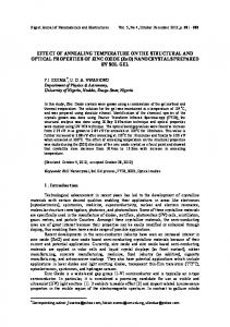
The round bar specimens with a length of 75 mm and diameter 15 mm for compressive deformation were cut from the steel pipe with the diameter × thickness of 1219 × 16.3 mm. The simulated TMCP was conducted in a Gleeble 3500 system, the schedules of which were given in Figure 1. Once reheated at 1180 ◦ C for 10 min, all deformation schedules are applied: a simulated “roughing” step is performed at a temperature of 1080 ◦ C with a compressive stain of 35% in the γ recrystallization region and an additional “finishing” step is performed at the temperature ranging from 850 to 790 ◦ C, using a compressive stain of 30%. Accelerated Cooling (ACC) started at 780 ◦ C with a 15 ◦ C/s cooling rate, then was interrupted at 200 ◦ C and followed by the simulated air cooling. Expansion curves (Figure 2) were also simultaneously measured during accelerated cooling, indicating that for the samples with a varying final rolling temperature from 850 to 790 ◦ C, the transformation of γ → α started at 530–586 ◦ C, and all the deformations took place in the single austenite field. To determine the austenite non-recrystallization temperature, Tnr , two-stage compression tests were performed in the Gleeble 3500 system where a compressive strain of 30% per each pass was applied to a group of samples of Φ10 × 15mm, with varying time intervals of 1–500 s between two passes, and temperature decreased from 1100 ◦ C to 700 ◦ C. The fraction of recrystallized grain was determined via quantitative metallography and plotted in Figure 3, as functions of deformation temperature and interval time, indicating that the Tnr is below 900 ◦ C, and the finish rolling temperatures were situated in the non–recrystallization region.
Metals 2016, 6, 323
3 of 16
Metals 2016, 6, 323 Metals 2016, 6, 323
3 of 16 3 of 16
Figure 1. Graph of the simulated TMCP (thermo mechanical control process) on the Gleeble for the steel with different finish rolling temperatures. Figure 1. Graph of the simulated TMCP(thermo mechanical control the the for the (thermo mechanical process) on on Gleeble Figure 1. Graph of the simulated TMCP control process) Gleeble for the steel finish rolling temperatures. with different steel with different finish rolling temperatures.
Figure curves andAr3 Ar3and Ar1 points with rolling 2. Expansion and Ar1 points for different finish Figure 2. Expansion curves and Ar3 and Ar1 points finish rolling 2. Expansion curves and forthe thesamples samples with different ◦ C°C ◦ C/s. temperatures of 850–790 and identicalcooling cooling rate temperatures of 850–790 ananidentical rateof of15 15°C/s. °C and °C/s.
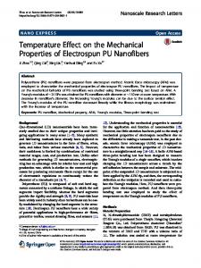
Figure 3. The fractions of recrystallized grains as functions of a varying finish rolling temperature and interval time between two passes.
Figure 3. 3. The The fractions fractionsofofrecrystallized recrystallizedgrains grains functions a varying finish rolling temperature Figure asas functions of aofvarying finish rolling temperature and After the simulation process, samples for observation on metallographic were cut the plane and interval time between two passes. interval time between two passes. perpendicular to the axis of compression, and carefully prepared according to the standard method. For examination of theprocess, microstructure by for Electron Microscope (SEM, Hitachi, Scanning After the simulation samples metallographic observation were cut onTokyo, the plane
After the simulation process, samples for metallographic observation were cut on the plane perpendicular to perpendicular to the the axis axis of of compression, compression, and and carefully carefully prepared prepared according according to to the the standard standard method. method. For examination of the microstructure by Scanning Electron Microscope (SEM, Hitachi, Tokyo, For examination of the microstructure by Scanning Electron Microscope (SEM, Hitachi, Tokyo, Japan), a 4% nital solution was used. To observe the M/A constituent, the Lepera’s reagent of 1 g sodium
Metals 2016, 6, 323
4 of 16
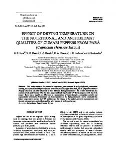
Japan), a 4% nital solution was used. To observe the M/A constituent, the Lepera’s reagent of4 1of g16 Metals 2016, 6, 323 sodium metabisulfite in 100 mL distilled water mixed with 4 g of picric acid dissolved in 100 mL of alcohol was used. By this way, M/A constituent (white) and ferrite (grey phase) can be identified metabisulfite in 100 mL distilled water with Oberkochen, 4 g of picric acid dissolved in 100 mL of of alcohol totally by an Optical Microscope (OM, mixed Carl Zeiss, Germany). Measurements size was used. By this way, M/A constituent (white) and ferrite (grey phase) can be identified totally an and area fraction of M/A constituent were performed mainly using image analysis withbythe Optical Microscope Carl Zeiss, Oberkochen, Germany). size and area fraction software Image-Pro (OM, Plus (Media Cybernetics, Rockville, MD, Measurements USA). For eachofspecimen, at least 10 of M/A constituent were performed mainly using image analysis with the software Image-Pro Plus fields of view containing at least 1000 particles were measured at a magnification of 2000×. Thin (Media MD, USA). were For each specimen, at the leasttwin-jet 10 fields of viewand containing at foils for Cybernetics, transmissionRockville, electron microscopy prepared using method observed least 1000 particles were measured at a magnification of 2000×. Thin foils for transmission electron in a JEM-2010 high-resolution transmission electron microscope (TEM, JEOL, Tokyo, Japan). The microscopy were prepared using the twin-jet method and observed in a JEM-2010 high-resolution carbon extraction replica technique was used to identify the morphology and size distribution of transmissionQuantitative electron microscope (TEM, JEOL, Tokyo, Japan). The were carboncarried extraction technique precipitates. measurements of precipitate particles out replica by using image was used to identify the morphology and size distribution of precipitates. Quantitative measurements analysis on a TEM image. The average size and fraction of precipitate particles were statistically of precipitate particles were carried out by using image analysis on containing a TEM image. The500 average size measured by averaging at least 1000 particles and five fields of view at least particles and fraction of precipitate particles were statistically by averaging at least 1000 particles and from the images of TEM, respectively. Electron back measured scattered diffraction (EBSD) examinations were five fields of view containing at least 500 particles from the images of TEM, respectively. Electron back performed on a Hitachi S-3400 Scanning Electron Microscope (SEM, Hitachi, Tokyo, Japan) scattered with diffraction (EBSD) examinations were performed onout a Hitachi Scanning Electron equipped a TSL EBSD system. The EBSD scan was carried with a S-3400 step size of 0.20 μm, and Microscope (SEM, Hitachi, Tokyo, Japan) equipped with a TSL EBSD system. The EBSD scan the EBSD effective grain size against tolerance angle ranging from 2° to 30° was calculated as was the carried outcircle withdiameter a step size of 0.20 µm,individual and the EBSD grain size tolerance angle equivalent related to the grain effective area. Moreover, the against dislocation density for ranging fromwas 2◦ to 30◦ was calculated as the equivalent circle diameter relatedThe to the individual each sample determined via quantitative X-ray diffraction (XRD) analysis. XRD spectra grainobtained area. Moreover, the dislocation density for each sample was determined via quantitative were by scanning in a Rigaku D/max-2500/PC diffractometer (Rigaku, Tokyo, Japan) X-ray over diffraction (XRD) analysis. The XRD spectra were obtained by scanning in a Rigaku D/max-2500/PC a scanning angle (2θ) range and step size of 35°–105° and 0.02°, respectively with unfiltered Cu Kα ◦ and diffractometer (Rigaku, Tokyo, Japan) over a scanningmethod angle (2θ) rangeon andthe step size of[14,24] 35◦ –105 radiation. The X-ray dislocation density measuring is based theory below. ◦ 0.02 , respectively with unfilteredby Cuthe Kα presence radiation.of The X-ray dislocation measuring method Diffraction peaks are broadened non-uniform strainsdensity that systematically shift is based on their the theory below. peaks broadeneddiffracting by the presence of non-uniform atoms from ideal [14,24] positions, andDiffraction by the finite size are of coherently domains. These two strainshave that asystematically shift atoms from theirofideal positions, and by the finite coherently effects different dependence on the value θ. The non-uniform strain effectsize canof therefore be diffracting domains. These two effects have a different dependence on the value of θ. The non-uniform separated, since the slope of a plot of βhkl cos{θhkl} versus 4sin{θhkl} is equal to a measure of the strain effect can therefore be separated, the slopepeak of a plot of βhkl cos{θhkl } versus 4sin{θhkl } is non-uniform strain ε. The parameter β is since the measured broadening. equal to a measure of the non-uniform strain ε. The parameter β is the measured broadening. The micro–tensile test [25–27] specimens were wire–cut according to Figure peak 4 from the TMCP The micro–tensile test [25–27] specimens were wire–cut according to Figure 4 from the TMCP treated samples and tensile tested on an Inspekt Table tensile testing machine at room temperature treated samples and tensile tested onmin an −1 Inspekt Table tensile testing machine at room temperature with a cross–head speed of 0.25 mm· . For each simulated process, three tensile samples were −1 . For each simulated process, three tensile samples were with a cross–head speed of 0.25 mm · min tested, and the yield strength was determined by the 0.2% offset flow stress. tested, and the yield strength was determined by the 0.2% offset flow stress. 17 1
2
2
8 2
R1.5
Figure 4. Wire-cut tensile specimens (in mm) from the center of the bar specimens along the Figure 4. Wire-cut tensile specimens (in mm) from the center of the bar specimens along the transversal direction. transversal direction.
3. Experiment Results 3. Experiment Results 3.1. Tensile Properties 3.1. Tensile Properties The tensile properties of specimens varied with the finish rolling temperature, and are shown in The properties of specimens varied with finish temperature, andthe aredecreasing shown in Figure 5.tensile It is indicated that the yield strength and the yield ratiorolling (YR) all increase with Figure 5. It is indicated that the yield strength and yield ratio (YR) all increase with the decreasing finish rolling temperature, whereas the tensile strength keeps steady. The YR, which equals to the ratio finish rolling temperature, whereas theistensile strength criterion keeps steady. The YR, which equals to the of yield strength and tensile strength, a subordinate for expression of strain hardening. A lower YR represents a better strain hardening capacity.
Metals 2016, 6, 323 Metals 2016, 6, 323
of 16 5 of516
Metals 2016, 6, 323 5 of 16 ratio of yield strength and tensile strength, is a subordinate criterion for expression of strain hardening.
ratio of yield strength and tensile strength, is a subordinate criterion for expression of strain hardening. A lower YRYR represents capacity. A lower representsa abetter betterstrain strainhardening hardening capacity.
Figure 5. Results of the tensile tests, as a function of the finish rolling temperature. Figure finish rolling rolling temperature. temperature. Figure 5. 5. Results Results of of the the tensile tensile tests, tests, as as aa function function of of the the finish
3.2. Microstructure 3.2. Microstructure 3.2. Microstructure The typical SEM micrographs of specimens as a function of the finish rolling temperature are The typical SEM 6. micrographs of specimens as atransformed function of of the the finish rolling rolling all temperature are shown in Figure It is confirmed that the microstructures consist ofare The typical SEM micrographs of specimens as a function finish temperature shown in Figure 6. It is confirmed that the transformed microstructures all consist quasi-polygonal (QF) and that granular bainitic ferrite (GF) with dispersed islands of secondary of shown in Figure 6. ferrite It is confirmed the transformed microstructures all consist of quasi-polygonal quasi-polygonal ferrite (QF) and granular bainitic (GF) with dispersed phases (mainly M/A constituent) in the ferrite matrix. Based on islands the researches byislands Xiao phases et of al. secondary [16–18], ferrite (QF) and granular bainitic ferrite (GF) withferrite dispersed of secondary (mainly phases (mainly M/A constituent) in the ferrite matrix. Based on the researches by Xiao et al. [16–18], this complicated intermediate transformation microstructure is defined as acicular ferrite (AF). The M/A constituent) in the ferrite matrix. Based on the researches by Xiao et al. [16–18], this complicated corresponding microstructure phases have been marked in the SEM micrographs of this study this complicated intermediate transformation microstructure is defined as acicular ferrite (AF). The intermediate transformation microstructure is defined as acicular ferrite (AF). The corresponding (Figure 6). corresponding phases microstructure have been marked in the ofSEM microstructure have beenphases marked in the SEM micrographs this micrographs study (Figure of 6). this study (Figure 6).
Figure 6. 6. The SEM differentfinish finishrolling rollingtemperatures: temperatures: Figure The SEMmicrographs micrographsfor forthe thespecimens specimens with different (a)(a) 850850 °C;◦ C; ◦ C; (c) 810 ◦ C and (d) 790 ◦ C. QF—quasi polygonal ferrite, GF—granular bainitic ferrite and (b)(b) 830830 °C; (c) 810 °C and (d) 790 °C. QF—quasi polygonal ferrite, GF—granular bainitic ferrite and M/A—martensite/austenite. M/A—martensite/austenite. Figure 6. The SEM micrographs for the specimens with different finish rolling temperatures: (a) 850 °C; (b) 830 °C; (c) 810 °C and (d) 790 °C. QF—quasi polygonal ferrite, GF—granular bainitic ferrite and The typical bright field TEM micrographs of specimens as a function of the finish rolling M/A—martensite/austenite.
temperature are presented in Figure 7. In general, the microstructure is predominantly composed of
Metals Metals 2016, 6, 3236, 323 2016,
6 of 166 of 16
The typical bright field TEM micrographs of specimens as a function of the finish rolling
non-equiaxed ferrite grains with martensite/austenite (M/A) islands at grain boundaries based temperature are presented in Figure 7. In general, the microstructure is predominantly composed of on grains with martensite/austenite (M/A) islands at grain boundaries based on are TEM non-equiaxed observations.ferrite It is revealed that both ferrite grains (white/grey) and M/A islands (black) TEM observations. It is decreasing revealed that ferrite grains (white/grey) and M/A islands (black) are significantly refined when theboth finish rolling temperature. significantly refined when decreasing the finish rolling temperature.
Figure 7. The TEM images of the typical microstructure morphology in the specimens with different
Figure 7. The TEM images of the typical microstructure morphology in the specimens with different finish rolling temperatures: (a) 850 °C; (b) 830 °C; (c) 810 °C and (d) 790 °C. finish rolling temperatures: (a) 850 ◦ C; (b) 830 ◦ C; (c) 810 ◦ C and (d) 790 ◦ C.
Figure 8 shows the morphology variation of M/A constituent with the finish rolling temperature. It can seen that thevariation coarse M/A constituent exists primarily the grain boundaries Figure 8 shows thebe morphology of M/A constituent with theatfinish rolling temperature. partM/A of ferrite, with theexists finishprimarily rolling temperature of boundaries 850 °C and 830 °C (Figure It canofbeprior seenaustenite that the and coarse constituent at the grain of prior austenite 8a,b). When the finish rolling temperature is 810 °C, M/A constituent disperses at the ferrite ◦ ◦ and part of ferrite, with the finish rolling temperature of 850 C and 830 C (Figure 8a,b). When the boundaries and its size becomes smaller (Figure 8c). When the finish rolling temperature decreases finish rolling temperature is 810 ◦ C, M/A constituent disperses at the ferrite boundaries and its size to 790 °C, M/A constituent becomes even smaller and distributes more dispersedly with the refined becomes smaller (Figure 8c). When the finish rolling temperature decreases to 790 ◦ C, M/A constituent ferrite grain (Figure 8d). As shown in Table 2, the amount of M/A constituent increases with the becomes even smaller and temperature, distributes more dispersedly with the refined(MED) ferritedecreases. grain (Figure 8d). decreasing finish rolling while their mean equivalent diameter As shown in Table 2, the amount of M/A constituent increases with the decreasing finish rolling Table 2. Results of the microstructural quantification. temperature, while their mean equivalent diameter (MED) decreases. Low Angle Boundaries (2°≤ θ < 15°) Finish Rolling M/A Constituent M/A Table(%) 2. Results of the microstructural quantification. Temperature (°C) Constituent MED (μm) Mean Misorientation (°) Fraction 850 4.5 ± 0.3 1.7 ± 0.2 6.2 ± 0.2 0.40 ± 0.02 830 5.4 ± 0.4 1.5 ± 0.3 ± 0.1 Boundaries0.41 0.01 Low6.2 Angle (2◦± ≤ θ < 15◦ ) Finish Rolling M/A M/A Constituent 810 6.3 ± 0.3 1.2 ± 0.2 6.1 ± 0.2 0.43 ± 0.01 ◦ Temperature ( C) Constituent MED (µm) (%) Mean6.1 Misorientation (◦0.44 ) ± 0.02 Fraction 790 7.4 ± 0.2 0.8 ± 0.1 ± 0.1
850 4.5 ± 0.3 1.7 ± 0.2 6.2 ± 0.2 0.40 ± 0.02 M/A—martensite/austenite and MED—mean equivalent diameter. 830 5.4 ± 0.4 1.5 ± 0.3 6.2 ± 0.1 0.41 ± 0.01 The has purpose of characterizing 810 EBSD technique 6.3 ± 0.3been applied for 1.2 the ± 0.2 6.1 ± 0.2and quantifying 0.43 ±the 0.01 microstructure. The misorientation angle figures of specimens with different finish rolling 790 7.4 ± 0.2 0.8 ± 0.1 6.1 ± 0.1 0.44 ± 0.02
temperatures are shown in Figure 9. The EBSD effective grainequivalent size for the ferrite matrix obtained by M/A—martensite/austenite and MED—mean diameter.
The EBSD technique has been applied for the purpose of characterizing and quantifying the microstructure. The misorientation angle figures of specimens with different finish rolling temperatures are shown in Figure 9. The EBSD effective grain size for the ferrite matrix obtained by different finish
Metals 2016, 6, 323 Metals 2016, 6, 323
7 of 16 7 of 16
Metals 2016, 6, 323 different finish rolling temperature been plotted Figure 10,ofasthe a function of the misorientation rolling temperature has been plottedhas in Figure 10, as in a function misorientation angle.7 of It 16 seems angle. Ittheseems clear that the mean equivalent diameter (MED) increases of the ferrite matrix increases clear that mean equivalent diameter (MED) of the ferrite matrix monotonically with the different finish rolling temperature has been plotted in Figure 10, as a function of the misorientation monotonically with the misorientation angle and the finish rolling temperature. misorientation angleclear and the rolling temperature. angle. It seems thatfinish the mean equivalent diameter (MED) of the ferrite matrix increases
monotonically with the misorientation angle and the finish rolling temperature.
Figure The M/A constituent observations finish rolling temperatures etched thethe Figure 8. 8. The M/A constituent at differentfinish finishrolling rolling temperatures etched by Figure 8. The M/A constituentobservations observations at at different different temperatures etched byby the ◦ C; ◦°C; ◦°C ◦ C. Ferrite Lepera’s reagent: (a) 850 °C; (b) 830 (c) 810 and (d) 790 °C. matrix is grey and M/A Lepera’s reagent: (a) 850 (b) 830 C; (c) 810 C and (d) 790 Ferrite matrix is grey and Lepera’s reagent: (a) 850 °C; (b) 830 °C; (c) 810 °C and (d) 790 °C. Ferrite matrix is grey and M/AM/A constituent white. M/A—martensite/austenite. constituent is is white. M/A—martensite/austenite. constituent is white. M/A—martensite/austenite.
Figure 9. The (electron back-scattered misorientation angle figures of specimens the specimens Figure 9. EBSD The EBSD (electron back-scattered diffraction) diffraction) misorientation angle figures of the ◦°C; ◦ C;(c)(c) ◦and ◦ C. The with different finish rolling temperatures: (a) 850 (b) 830 °C; 810 °C (d) 790 °C. The red red with different finish rolling temperatures: (a) 850 C; (b) 830 810 C and (d) 790 Figure 9. The EBSD (electron back-scattered diffraction) misorientation angle figures of the specimens ◦ –15◦ and greater than line and the black line represent the misorientation angle in the range 2 with different finish rolling temperatures: (a) 850 °C; (b) 830 °C; (c) 810 °C and (d) 790 °C. The red 15◦ , respectively.
Metals 2016, 6, 323
8 of 16
line and the black line represent the misorientation angle in the range 2°–15° and greater than 15°, 8 of 16 respectively.
Metals 2016, 6, 323
Figure 10. ferrite matrix, as aasfunction of the misorientation angleangle and 10. The The EBSD EBSDmean meaneffective effectivesize sizeofof ferrite matrix, a function of the misorientation finish rolling temperature. MED—mean equivalent diameter. and finish rolling temperature. MED—mean equivalent diameter.
3.3. Precipitation
TEM micrographs micrographs and EDS EDS analysis analysis of the the representative representative Figure 11 shows the bright field TEM precipitates observed observed in the the specimens specimens with with different different finish finish rolling rolling temperatures. temperatures. The observed observed precipitates different size precipitates can can be be classified classified into two different size ranges: ranges: 10–30 nm (fine precipitates) and 30–100 nm precipitates precipitates),shown shown in Table The smallest size range nm) are precipitates are (coarse precipitates), (coarse in Table 3. The3.smallest size range (10–30 nm)(10–30 precipitates niobium-rich niobium-rich while 30–100 spherical nm cuboidal, spherical and irregular precipitates and are carbides, whilecarbides, 30–100 nm cuboidal, and irregular precipitates are titanium-rich titanium-rich and niobium-contained (Ti, it Nb)C. Moreover, can be that there are quite a lot of niobium-contained (Ti, Nb)C. Moreover, can be seen thatitthere areseen quite a lot of fine precipitates ◦ C (Figure fine precipitates present in the ferrite finish rolling temperature is 11a), 850 °C (Figure present in the ferrite matrix when thematrix finish when rollingthe temperature is 850 while the ◦ 11a), while the amount decreases a little at a finish rolling temperature of 830 °C (Figure 11b). When the amount decreases a little at a finish rolling temperature of 830 C (Figure 11b). When the finish ◦ finish rolling temperature °C,ofplenty coarse precipitates present inmatrix the ferrite matrix rolling temperature is 810 is C, 810 plenty coarseofprecipitates are presentare in the ferrite (Figure 11c). (Figurethe 11c). When thetemperature finish rollinglowers temperature to 790 °C, the amount of coarse precipitates When finish rolling to 790 ◦lowers C, the amount of coarse precipitates becomes even becomes even larger larger (Figure 11d). (Figure 11d).
Figure 11. 11. The precipitates obtained obtained from from the the specimens specimens with with Figure The TEM TEM micrographs micrographs of of the the representative representative precipitates ◦ ◦ ◦ ◦ finish rolling rolling temperatures: temperatures: (a) (a) 850 850 °C; different finish (b) 830 830 °C; different C; (b) C; (c) 810 °C C and (d) 790 °C. C.
Metals 2016, 6, 323
9 of 16
Metals 2016, 6, 323
9 of 16
Table Table 3. 3. Classification Classification of of different different precipitates precipitates in in the the test testmicroalloyed microalloyedsteel. steel.
Precipitate Precipitate
Morphology Morphology Spherical/Irregular Spherical/Irregular Cuboidal Cuboidal Spherical Spherical
Ti-rich (Ti,Nb)C Nb)C Ti-rich (Ti, Nb-rich (Nb, Nb-rich (Nb,Ti)C Ti)C
SizeRange Range (nm) Size (nm) 30–100 30–100 10–30 10–30
Quantification analyses inin Figure 12 12 and Table 4. It4.isItrevealed that Quantification analyses of ofthe theprecipitates precipitatesare areshown shown Figure and Table is revealed the amount of the fine precipitates (10–30 nm) decreases (Figure 12), while the average size of that the amount of the fine precipitates (10–30 nm) decreases (Figure 12), while the average size of precipitate particles increases when decreasing the finish rolling temperature (Table 4). precipitate particles increases when decreasing the finish rolling temperature (Table 4).
Figure 12. 12. Percent Percent distribution distribution of of precipitate precipitate particles particles of of different different size size in in the the specimens specimens varied varied with with Figure finish rolling rolling temperature. temperature. finish Table4.4.Average Averageprecipitate precipitate size precipitation volume fraction the specimens with Table size andand precipitation volume fraction of theofspecimens variedvaried with finish finish rolling temperature. rolling temperature.
Finish Rolling Temperature (°C) 850 850 830 830 810810 790790
Finish Rolling Temperature (◦ C)
x (nm) 29.3 ± 0.1 29.3 ± 0.1 33.6 ± 0.2 33.6 ± 0.2 48.248.2 ± 0.2± 0.2 50.350.3 ± 0.1± 0.1
Volume Fraction f 10.8 ± 0.2 × 10⁴−4 10.8 ± 0.2 × 10−−4 9.4 ± 0.1 × 10 9.4 ± 0.1 × 10⁻⁴ −4−4 8.18.1 ±± 0.30.3 × ×1010 − 4−4 ± 0.1 7.67.6 ± 0.1 ×× 1010
x (nm)
Volume Fraction f
x—average size,f —volume f—volume fraction. x—averageprecipitate precipitate size, fraction.
3.4. Dislocations 3.4. Figure 13 13 shows shows the the XRD XRD patterns patterns corresponding corresponding to samples samples with different finish finish rolling rolling Figure temperatures, and the dislocation dislocation densities densities are are summarized summarized in in Table Table 5.5. As the table table shows, shows, the the temperatures, density of dislocations, ρ, increased with the decreasing finish rolling temperature. density of dislocations, ρ, increased with the decreasing finish rolling temperature. Table 5. The density of dislocations of samples varied with a finish rolling temperature from 850 ◦ C to 790 ◦ C. Finish Rolling Temperature (◦ C)
ρ/× 1014 m−2
850 830 810 790
5.2 ± 0.05 5.9 ± 0.04 6.7 ± 0.07 7.2 ± 0.07
Note: ρ-The average dislocation density.
x—average precipitate size, f—volume fraction.
3.4. Dislocations Figure 13 shows the XRD patterns corresponding to samples with different finish rolling temperatures, the Metals 2016, 6, 323 and the dislocation densities are summarized in Table 5. As the table shows, 10 of 16 density of dislocations, ρ, increased with the decreasing finish rolling temperature.
Figure 13. XRD (X-ray diffraction) spectra of samples varied with a finish rolling temperature from 850 ◦ C to 790 ◦ C.
4. Discussion 4.1. Effect of Finish Rolling Temperature on Microstructure Evolution The microstructure evolution can be explained as follows. The rolling in the austenite recrystallization region brings about a continuous recrystallization of austenite grains during the rolling process and this can remarkably refine the austenite grain size [28]. Subsequently, high densities of substructure and dislocation (deformation bands) are generated in the austenite when the rolling is conducted in the non-recrystallized austenite region [29]. During the following continuous cooling process, the deformed austenite transforms into ferrite continuously, and the retained austenite is further carbon-enriched and fully stabilized until the transformation becomes thermodynamically impossible [30]. Finally, part of the carbon-enriched retained austenite could transform to martensite and the retained austenite would coexist with the martensite, making the so-called M/A constituent [31]. It is universally acknowledged that the rolling temperature plays an important role in the grain refinement and precipitation hardening by affecting prior austenite grain structure, precipitation of coarse carbides (strain induced precipitation) and dislocation substructure [22]. Because the austenite grain boundaries and deformation bands can act as the nucleation sites for austenite/ferrite phase transformation, grain refinement is enhanced with the increase of austenite grain boundary and dislocation density [32,33]. With the decreasing finish rolling temperature in the non-recrystallized austenite region, more and more deformation dislocations would be accumulated, therefore significant grain refinement has been achieved (Figure 8). On the other hand, there occur two groups of precipitates, i.e., fine and coarse ones, in the final matrix. The coarse precipitates are made up of the Ti-rich particles, probably survived from reheating due to their high thermodynamic stability; and the Nb-rich ones, primarily coming from the strain induced precipitation in the austenite non-recrystallization zone. The well-developed dislocation structure inside the austenite grain promotes the precipitation kinetics [34]. Such strain induced precipitates will grow during the remaining process, and consequently become coarse precipitates (>30 nm). Meanwhile, the precipitation of fine articles with 10–30 nm might mainly take place during controlled cooling. Due to the precipitation of coarse carbides since the rolling process, which consumes carbide formers—Nb, Ti and C—fine precipitates (10–30 nm) are significantly reduced during the subsequent continuous cooling process. It is revealed that the amount of coarse precipitates increases with the decreasing finish rolling temperature, while the amount of fine precipitates reduces accordingly (Figures 9 and 10), leading to the decreasing average precipitate size. This is consistent with the observations made by Olalla et al. [21] and Kostryzhev et al. [23]. Moreover, the M/A constituent increases in amount, and decreases in size, as well as distributing more dispersedly while decreasing the finish rolling temperature (Figures 7 and 8 and Table 2).
Metals 2016, 6, 323
11 of 16
According to previous work [35], a sufficient deformation strain of Fe–0.43C–3Mn–2.12Si (wt %) steel can lead to a mechanical stabilization of austenite to some degree, and accordingly lower the onset temperature of bainitic transformation. However, for the present experimental steel, the decreasing finish rolling temperature corresponds to an elevated onset temperature (Ar3 ) of γ → QF + GF (Figure 2), indicating that the initial stability of deformed austenite is reduced, possibly due to the increased dislocation substructure acting as the nucleation site for QF and GF. Nevertheless, the continuous cooling phase transformation of γ → α + γ’ (metastable austenite) is accompanied by the partitioning of carbon atoms from α to γ’ through the dislocation related pipe diffusion and bulk diffusion [22,34], resulting in C-rich γ’ with correspondingly elevated stability. Therefore, it could be proposed that due to the decreasing finish rolling temperature, the increased dislocation structure would enhance the stability of austenite during the subsequent continuous cooling transformation, and accordingly result in an increasing amount of M/A constituent. Simultaneously, locations for M/A constituent at the ferrite boundaries become more scattered and their size decreases because of grain refinement. 4.2. Effect of Finish Rolling Temperature on Tensile Properties The yield strength of Nb–Ti microalloyed pipeline steel can be described by a linear sum of the individual strengthening contributions; i.e., σy = σ0 + σs + σd + σdis +σph + σM-A
(1)
where σ0 : lattice friction stress; σs : solid solution strengthening, owing to interstitial and substitutional atoms; σd : strengthening provided by the boundaries of the GBF (granular bainitic ferrite) and AF effective grain; σdis : dislocation strengthening of the GBF and AF; σph : carbonitride precipitation strengthening; σM-A : strengthening owing to the hard M/A constituent. The YS (yield strength) is affected by each of these strengthening factors in varying degrees. For the present study, the values of these strengthening factors are calculated to better understand the strengthening mechanism of the experimental steel. The calculation of grain boundary strengthening is by the Hall–Petch equation, based on the EBSD test results. According to [36], the lowest threshold angle that provides a consistent crystallite size quantification from EBSD scans has been estimated experimentally at 2◦ , irrespective of the type of microstructure. Moreover, the contribution of very low angle boundaries with a misorientation θ < 2◦ to strength can be regarded as part of the total dislocation strengthening, while the rest of boundaries with a misorientation θ ≥ 2◦ contribute to the boundary strengthening. In this attempt, the EBSD effective size corresponds to the boundaries with a misorientation 2◦ ≤ θ ≤ 30◦ . In detail, high angle boundaries (θ ≥ 15◦ ) are relevant to the bainitic packets/sheaves, according to [36], while low angle boundaries (2◦ ≤ θ < 15◦ ) are related to the ferrite sub-units within the bainitic packets/sheaves. High angle boundaries (θ ≥ 15◦ ) are expected to contribute with an orientation independent Hall–Petch coefficient, kHP , while the strength of low angle boundaries (2◦ ≤ θ < 15◦ ) depends on the misorientation [37]:
√ kHP (θ) = kαMµ bθ
(2)
in which k is a proportionality constant of the order of 1, while α, M, µ and b represent a constant, the Taylor factor, the shear modulus and the Burgers vector, respectively [37]. The following expression has been recently deduced [36]: σd = kHP (MED2◦ )
−0.5
√ ∼ = 1.05αMµ b
"
∑
2◦ ≤θi