Effects of climate change on phenologies and ... - Wiley Online Library

Effects of climate change on phenologies and distributions of bumble bees and the plants they visit Graham H. Pyke,1,2,3,4,† James D. Thomson,4,5 David W. Inouye,4,6 and Timothy J. Miller7 1School

of the Life Sciences, University of Technology Sydney, Broadway, New South Wales, Australia 2Australian Museum, Sydney, New South Wales, Australia 3Department of Biology, Macquarie University, Ryde, New South Wales, Australia 4Rocky Mountain Biological Laboratory, P. O. Box 519, Crested Butte, Colorado 81224 USA 5Department of Ecology and Evolutionary Biology, University of Toronto, Toronto, Ontario M5S 3G5 Canada 6Department of Biology, University of Maryland, College Park, Maryland 20742 USA 7Department of Ecology and Evolutionary Biology, University of California, Santa Cruz, California USA Citation: Pyke G. H., J. D. Thomson, D. W. Inouye, and T. J. Miller. 2016. Effects of climate change on phenologies and distributions of bumble bees and the plants they visit. Ecosphere 7(3):e01267. 10.1002/ecs2.1267

Abstract. Surveys of bumble bees and the plants they visit, carried out in 1974 near the Rocky Mountain

Biological Laboratory in Colorado, were repeated in 2007, thus permitting the testing of hypotheses arising from observed climate change over the intervening 33-yr period. As expected, given an increase in average air temperature with climate warming and a declining temperature with increasing elevation, there have been significant shifts toward higher elevation for queens or workers or both, for most bumble bee species, for bumble bee queens when species are combined, and for two focal plant species, with no significant downward shifts. However, contrary to our hypotheses, we failed to observe significant altitudinal changes for some bumble bee species and most plant species, and observed changes in elevation were often less than the upward shift of 317 m required to maintain average temperature. As expected, community flowering phenology shifted toward earlier in the season throughout our study area, but bumble bee phenology generally did not change, resulting in decreased synchrony between bees and plants. However, we were unable to confirm the narrower expectation that phenologies of bumble bee workers and community flowering coincided in 1974 but not in 2007. As expected, because of reduced synchrony between bumble bees and community flowering, bumble bee abundance was reduced in 2007 compared with 1974. Hence, climate change in our study area has apparently resulted primarily in reduced abundance and upward shift in distribution for bumble bees and shift toward earlier seasonality for plant flowering. Quantitative disagreements between climate change expectations and our observations warrant further investigation.

Key words: altitudinal transect; asynchrony; Bombus; bumble bee; community ecology; elevation; flowering; pollination; reproduction; Rocky Mountain Biological Laboratory. Received 16 June 2015; revised 23 June 2015; accepted 29 June 2015. Corresponding Editor: D. P. C. Peters. Copyright: © 2016 Pyke et al. This is an open access article under the terms of the Creative Commons Attribution License, which permits use, distribution and reproduction in any medium, provided the original work is properly cited. † E-mail: [email protected]

Introduction

climate zones (Forister et al. 2010, Bedford et al. 2012, Roth et al. 2014). Consistent with global warming (Parmesan 2006), for example, the distributions of a wide range of species have shifted toward higher latitudes (Nakamura et al. 2013,

Organisms are expected to respond to changing climate by shifting geographical ranges and phenology toward remaining in their compatible v www.esajournals.org

1

March 2016 v Volume 7(3) v Article e01267

PYKE ET AL.

Cavanaugh et al. 2014, McCain and King 2014, Paprocki et al. 2014) and higher elevations (Narins and Meenderink 2014, Pizzolotto et al. 2014, Urli et al. 2014), and there have been phenological shifts toward earlier spring events (Dunn and Moller 2014, Polgar et al. 2014). Such changes may result in mismatches, either temporal or spatial, between interacting species (Tylianakis et al. 2008), especially when they are from different trophic levels such as plants and their pollinators (Visser and Both 2005, Both et al. 2009). Plants and animals generally respond differently to climatic variables (Visser and Both 2005, Doi et al. 2008, Forrest and Thomson 2011, Parsche et al. 2011, Rafferty and Ives 2011, Kudo and Ida 2013) and so formerly synchronous plants and pollinators are likely to become asynchronous through shifts in the phenology of one relative to the other (Rafferty and Ives 2011, 2012, Willmer 2012, Kudo and Ida 2013). Pollinators may become seasonally active later relative to the plants they visit (Doi et al. 2008, McKinney et al. 2012), although no dislocation between plants and animals was found in one study (Bartomeus et al. 2011). It has similarly been found that breeding by birds may have become disrupted through a climate-induced temporal mismatch with food supply (Burger et al. 2012). However, we are not aware of any community-level study that has considered possible mismatches, arising from asynchronous climate-induced shifts in altitude, latitude or other spatial variable, in plants relative to their pollinators or among interacting species in general. The mutualistic relationship between plants and their pollinators, their long period of co- evolution, and the relatively little anthropogenic climate change that had occurred prior to about 40 yr ago, make it likely that synchrony between them should have been high up till then. More recent climate change, with associated global warming, has been much greater since then, with the period from 1983 to 2012 “likely the warmest 30-yr period of the last 1400 yr in the Northern Hemisphere” (IPCC 2013). There should therefore have been significant deterioration in plant- pollinator synchrony over about the last 40 yr. Although synchrony between plants and their pollinators should have declined, with increasing temporal disconnect between the two groups, the expected direction and magnitude v www.esajournals.org

of this temporal disconnect is unknown. We lack information concerning how animals and plants are responding to changing climate, and whether these two groups are responding synchronously (Miller-Rushing and Inouye 2009). Hence, while both groups are expected to have shifted toward being seasonally earlier, it is not possible to predict the relative magnitudes of these shifts, and so not possible to predict which group should have become seasonally earlier than the other, nor what the difference between the two groups should now be. However, other studies have so far mostly found that phenologies of the plants have shifted earlier by more than their animal pollinators, so that the animals are now late relative to the plants (Doi et al. 2008, Forrest and Thomson 2011, McKinney et al. 2012). As temporal mismatches between phenologies of plants and their pollinators have developed or increased, pollinator reproduction will likely have been reduced, leading to a decline in pollinator abundance. Times would have increasingly arisen in which there were either too few pollinators to take advantage of abundant flowering or too many relative to available floral resources (Rafferty and Ives 2011), with reduced pollinator reproduction occurring in both circumstances. Subsequently, reduced reproduction over successive years would have compounded, resulting in a decrease in pollinator abundance. Plant reproduction, and hence plant abundance, may also have declined as a result of decreased synchrony between plants and pollinators. If, for example, some plants are now flowering early relative to the timing of their pollinators, as has been reported in some cases (Doi et al. 2008, Forrest and Thomson 2011, McKinney et al. 2012), and their reproduction is limited by pollen receipt, then such plants could suffer reduced reproduction, resulting in their decreased abundance. Evolution of plant and pollinator phenologies could counteract any effects arising from decreased synchrony, but it seems unlikely that this would have occurred in long-lived perennials that characterize our study area, over the 33 yr of this study. A temporal disconnect between plants and their pollinators should favor, through natural selection, more synchronous individuals, for both plants and pollinators. However, any consequent evolutionary change in overall 2


PYKE ET AL.

not have influenced our comparison, as most of our sites were within National Forest and there were no apparent changes to land-use between 1974 and 2007 at any of the sites. We hypothesized that observed climate change in our study area during the 33-yr period between 1974 and 2007 would have affected bumble bees and plants as follows. Hypothesis 1: Species distributions have shifted upwards by about 317 m for both bumble bees and the plants on which they feed, matching the change in temperature with elevation. Consistent with increases in average temperature, a number of plant and animal species in our study area have shown evidence of the expected upward shifts (Perfors et al. 2003, synchrony between the two groups would re- Menke et al. 2014). However, none of these quire many generations. studies has tested whether the magnitudes of Studies of mountain ecosystems should be par- observed changes in elevation are quantitatively ticularly informative in terms of understanding as expected under climate change. effects of climate change. Organisms are more Both bumble bees and plants in our study likely to shift distributions in terms of altitude would have had to shift upwards in elevation than latitude, because of the shorter distances by 317 m to maintain an unaltered average temto track a particular climatic regime (Crimmins perature. The observed lapse rate at which averet al. 2009). Furthermore, mountain ecosystems age daily temperature during summer decreasare predicted to experience some of the earliest es with increasing elevation in a nearby area of and strongest effects of climate change (Nogués- central Colorado is about 6.3°C/1000 m (Meyer Bravo et al. 2007, Saunders et al. 2008), and ex- 1992). The observed increase in average monthly tinction risks associated with climate warming spring/summer temperature in the study area of are expected to be aggravated for species endem- about 2°C is therefore equivalent to a decrease in ic to mountainous areas, especially those restrict- elevation of 317 m (i.e., 1000 * 2/6.3 m). ed to the highest elevations (Dirnböck et al. 2011). Hypothesis 2: Bumble bee and flowering plant pheOn the other hand, because of the relatively short nologies have shifted toward earlier in the season, distances between areas of different elevation in but not identically, resulting in lost temporal synmountainous regions, short-term movements of chrony between them (It was not possible to predict organisms may mask or ameliorate effects of clithe direction or magnitude of this temporal disconnect mate change. Despite this, evidence is accumubetween bumble bees and plant flowering.). lating for both plants and pollinators that latitudinal and altitudinal ranges are changing (Roth Consistent with warming temperatures in our et al. 2014), and if they are not changing synchro- study area, events associated with spring have nously, there is the potential for altered interac- been occurring earlier, and so the phenologies tions among them (Rafferty and Ives 2012). of bumble bees and the plants they visit should We consider the possible effects of climate have shifted toward earlier in the season. Over change on a plant-pollinator system in the moun- the period between 1973 and 2006, the average tainous area around the Rocky Mountain Biolog- monthly air temperature recorded at the nearby ical Laboratory (RMBL) in Colorado, through town of Crested Butte (fig. 1 in Pyke et al. surveys of bumble bees and the flowers they visit 2012) during April-June has increased by an carried out initially in 1974 (Pyke 1982, Pyke et al. estimated 2.0°C (Miller-Rushing and Inouye 2011, 2012) and repeated in 2007. Direct human- 2009). Similar increases in average air temperainduced modification to the environment should ture have presumably occurred throughout the

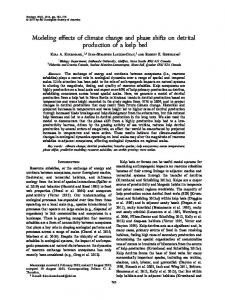
Fig. 1. Proportion of sites where Delphinium barbeyi was present vs. elevation region in 1974 and 2007.

v www.esajournals.org

3

March 2016 v Volume 7(3) v Article 1267

PYKE ET AL.

local area. Associated with such increased average temperatures, snowmelt in the area during spring/summer has tended to occur earlier (Miller-Rushing and Inouye 2009), and the activities of some plants and animals have shifted phenologically toward earlier in the season (Inouye et al. 2000, 2003, Miller-Rushing and Inouye 2009, Lambert et al. 2010). However, as discussed above, we currently have no basis for predicting changes in the phenology of one species relative to another.

circular areas spaced along-side roads (i.e., circle sites) and roughly rectangular lengths along walking tracks or routes between the main road and highest nearby elevations (i.e., transect sites). Sites along roads consisted of areas within about 50 m from central points, while sites along walking routes consisted of the areas within about 25 m on either side of the route for particular segments of the route. These walking segments were either determined naturally by changes in topography and vegetation along the route, or defined by elevation intervals of 500 ft (e.g., 10 500 to 11 000 ft, i.e., 3182 to 3333 m). Further information regarding these sites may be found in earlier publications (Pyke 1982, Pyke et al. 2011, 2012) and location details for these sites and walking routes have been archived at RMBL. This study considers 47 of the sites from 1974 that were re-surveyed in 2007. The identities and locations of all but one of these sites have been presented previously in Appendix Tables A2-1 and A2-2 in Pyke et al. (2012). The identities of those sites that were re-surveyed in 2007 are listed in the appendix to the current article, using previous location codes, along with details for one additional site that was surveyed in both years (see Appendix Section A1). The road-side circle sites traversed topography that was generally flatter and lower in elevation than the transect sites (Pyke et al. 2012; see Appendix Section A1 for details).

Hypothesis 3: Bumble bee abundance was lower in 2007 than in 1974. With increasing temporal disconnect between bumble bees and the plants they visit, we expected declines in bumble bee reproduction, and consequent declines in bumble bee abundance, as discussed above. Changes in abundance, consistent with climate change, have been observed in our study area for various species of plants (Harte and Shaw 1995, de Valpine and Harte 2001, Perfors et al. 2003, Saavedra et al. 2003, Harte et al. 2006, Miller-Rushing and Inouye 2009) and animals (Ozgul et al. 2010).

Methods Study area and sites

This study was carried out near the Rocky Mountain Biological Laboratory (RMBL) in Colorado, USA during 1974 and 2007. In this area elevations may vary by 1,000 m or more over only a few km of horizontal distance (fig. 1 in Pyke et al. 2012). The study area encompassed an elevation range of just over 1000 m from near the town of Crested Butte at 2693 m to mountain tops about 16 km to the north with maximum elevations of ≈3760 m (fig. 1 in Pyke et al. 2012). Within this area the woody vegetation was dominated by sagebrush at the lowest elevations, and by aspen and spruce-fir forest at higher elevations, with willows along streams. Our study focused on sites that were dominated by grasses and herbaceous plants, and occurred throughout the study area. Study sites were established in 1974 to cover the elevation range present in our study area, while using available trails and roads that provided site access and replication for elevation (Pyke 1982, Pyke et al. 2012). Sites consisted of both v www.esajournals.org

Bumble bee and flower surveys

Both years we surveyed as much of the summer flowering season as possible, at intervals sufficiently short to capture seasonal changes. During 1974 most sites were visited about every 8 d during the period between 22 June and 8 September (Pyke 1982); during 2007 they were visited about every 6 d between 20 June and 8 August. The difference in survey period meant that some data collected toward the end of the 1974 season could not be used in comparisons between the 2 yr (see below). Survey methods adopted in the 2 yr were essentially identical (Pyke 1982, Pyke et al. 2011, 2012). In both years, surveys were carried out at each site, generally between about 09:00 and 18:00. As a result of variation in daily start time, initial site, and sequence direction of surveyed sites along transects, each site was surveyed at different times of day over the course of each season.

4


PYKE ET AL.

B. flavifrons, B. frigidus, B. mixtus, B. occidentalis, B. sylvicola) as these species accounted in most cases for over 97% of recorded bumble bees, excluding Region 1, for all castes (i.e., queens, workers, males) in both years (Appendix: Table A1-1).

During survey visits to a site, one to three people walked within the site and separately recorded the identities of any bumble bees observed (i.e., species and caste), along with the identity of any visited flower. In addition, the identities of plant species in flower were recorded for each survey visit to a site. We adopt the plant species names of Hartman and Nelson (2001) and parenthetically include older names used in Pyke (1982). Except for two species of cuckoo bumble bee (B. insularis and B. suckleyi), all bumble bee species could be distinguished in the field (Pyke 1982, Pyke et al. 2011, 2012). Surveys in the 2 yr were also essentially identical in terms of site coverage and duration (See Appendix Section A1).

Measures of bumble bee and plant density

We assume that the number of bumble bees recorded per person hour (i.e., recording rate) is proportional to bumble bee density (Pyke et al. 2011, 2012), and considered each caste separately because they exhibited distinctly different phenologies, with spring queens seasonally earliest, followed by workers, and then males and autumn queens together at the end of the season. It is then relatively straightforward to consider how these recording rates are affected by other variables, such as species, caste, time of day, date period and elevation range (Pyke et al. 2011, 2012), and how these patterns may differ between years (see below). Of course, bumble bee recording rate does not measure actual density of bumble bees. As measures of plant density we took the proportions of sites, within each elevation region, at which particular plant species were recorded as present, as these proportions should be correlated with plant density and variation in them reflected known elevation distributions for the various plant species (e.g., Fig. 1). To compare the 2 yr, we therefore scored presence or absence (1 or 0) for each plant species at a particular site, calculated a presence change value by subtracting the presence score in 1974 from the score in 2007, and then used this presence change value as a dependent variable. In this case, for example, an average change in presence of −0.5 would mean that there had been a net disappearance between years across half the sites. Unfortunately, it was not possible to carry out transect or plot-based counts of flowers or plants in either year.

Spatial and temporal variables

To facilitate analyses, spatial and temporal variables were assigned to discrete categories. For spatial analysis, sites were categorized, as previously (Pyke 1982), into eight equal elevation regions of 500 vertical ft or 152 m (i.e., region 1 = 8500−9000 ft = 2576−2727 m; region 2 = 9000−9500 ft = 2727−2879 m; etc.). Surveys were also categorized into three roughly equal time periods (i.e., before 12 noon, 12 noon to 3 pm, after 3 pm), resulting in reasonable sample sizes for each category. Seasonal analyses were based on date periods that were the first and second halves of each month (e.g., date period 1 was 16–30 June, date period 2 was 1–15 July, etc.). Finer subdivisions of time resulted in too few observations for some date periods and no surveys for some site-period combinations.

Plant species

Twelve plant species in our study, all perennial (Treshow 1975), have been identified as being of particular importance to bumble bees, by virtue either of accounting for high proportions of bumble bees recorded visiting their flowers or being preferred by particular bumble bee species over other plant species (Pyke 1982). For sites surveyed during both 1974 and 2007, these plant species accounted for 74.5% of recorded bumble bees in each year (Table 1). We focus below on these species.

Phenologies

As representations of bumble bee and flowering phenologies, we took the seasonal patterns of bumble bee recording rate and number of plant species in flower, each reaching a peak during the summer season, but with different shapes to their seasonal pattern. Graphs of bumble bee recording rate over time typically

Bumble bee species

We focused on eight bumble bee species (i.e., B. appositus, B. balteatus [kirbyellus], B. bifarius, v www.esajournals.org

5


PYKE ET AL.

Table 1. Twelve plant species considered particularly important to bumble bees are listed in order of decreasing numbers of recorded bumble bees in 1974. Also presented for each of these species are the results of fitting the model CP = A + B*R + C*R2, where CP is change in presence between years, R is Elevational Region and A-C are unknown coefficients). Threshold for significance is P = 0.01. Plant Species

# Bumble bee records 1974

# Bumble bee records 2007

Delphinium barbeyi Hymenoxys (Helenium) hoopsii

2922 1369

800 100

Helianthella quinquenervis

1168

449

Mertensia ciliata Chamerion (Epilobium) angustifolium Aconitum columbianum

891 853

67 224

776

154

Senecio triangularis

695

17

Senecio bigelovii

605

107

Senecio crassulus

582

28

Viguiera multiflora

499

205

Phacelia leucophylla

359

58

Castilleja sulphurea

161

37

Total these species Total all species

10880 (74.5%) 14595

2246 (74.5%) 3013

B & C negative. No significant coefficients (P’s > 0.3) B & C negative. No significant coefficients (P’s > 0.02) B & C negative. No significant coefficients (P’s > 0.3) B & C positive. C = 0.012 (SE = 0.004, P = 0.003) B & C positive. No significant coefficients (P’s > 0.5) B & C negative. No coefficients significant (P’s > 0.2) B & C negative. No significant coefficients (P’s > 0.5) B & C negative. No significant coefficients (P’s > 0.1) B & C positive. No significant coefficients (P’s > 0.05) B & C negative. No significant coefficients (P’s > 0.4) B & C negative. No significant coefficients (P’s > 0.04) B & C positive. No significant coefficients (P’s > 0.04)

flower by assuming that the seasonal patterns of these recording rates are Gaussian and Quadratic functions of date period respectively, where the date of the peak is an unknown parameter. Hence, our models were of the forms BRR = A*EXP(−[P-C]2/B) and NPF = A + B*(P-C)2 respectively, where BRR is bumble bee recording rate, NPF is number of plant species in flower, P is date period, A-C are all unknown, and C is the date of the peak. We considered the possibilities that bumble bee recording rates and numbers of plant species in flower may have varied with Elevation Region (R) and Year, and their interaction, by allowing the unknowns to be functions of Ri,Y and RjY [i,j = 1,2], where Y equals Year/1000. The coefficients of these parameters, with associated standard errors, were estimated using nonlinear regression.

appear bell-shaped, increasing roughly exponentially until reaching maximum levels before declining, rapidly at first, then more slowly (Figs. 2 and 3). On the other hand, phenology in terms of number of plant species in flower (hereafter referred to as community flowering phenology) is generally shaped like an upturned U (Figs. 2 and 3). For both bumble bees and flowering, the dates of the peaks then provide comparative measures of their phenologies across elevation region and year. In the case of bumble bees, we considered queens and workers separately, as they have quite different phenologies, but combined species because earlier analysis had indicated that there are no phenological differences between species in our study area (Pyke et al. 2011). Because our surveys in 2007 ended seasonally earlier than in 1974, we were unable to consider male bumble bees. We focused on plant species used as sources of floral resources by bumble bees. We estimated dates of peak bumble bee recording rate and peak number of plant species in v www.esajournals.org

Directions and significance of coefficients, with probabilities and SE values

Allowance for differences in bumble bee phenology between regions and years

As bumble bee phenology varied with elevation region and year, comparisons of bumble

6


PYKE ET AL.

Fig. 2. Average numbers of plant species in flower and bumble bees recorded per person hour vs. time period for transect surveys carried out in 1974 and 2007.

Fig. 3. Average numbers of plant species in flower and bumble bees recorded per person hour vs. time period for circle surveys within regions 4–5 and carried out in 1974 and 2007.

bee abundance between elevation regions and years were based on the date periods for each region and year when maximum abundances were observed (Pyke et al. 2011). If, for example, a particular bumble bee species reached peak worker abundance at relatively low elevations during the second half of July, but did not reach peak worker abundance at higher elevations until later, then an analysis of the distribution of this bumble bee based on the second half of July would be biased toward the lower elevations. The same problem applies to comparing years if there are similar differences in phenology between years. It is therefore necessary to make phenological restrictions such that recording rates are maximal before comparing bumblebee recording rates across regions and years. However, rather than making separate phenological restrictions for each combination of year v www.esajournals.org

and elevation region, we simplified the process through adoption of a relatively small number of year/region/date period combinations (see Appendix Section A1 for explanation and Table A1- 2 for results). In addition, we separately considered spring queens and workers, but combined all bumble bee species, excluding the cuckoo bumble bees (see Appendix: Section A2).

Elevational distributions of bumble bees and plants

We assumed that recording rates for bumble bee workers (after phenological adjustment as described above) varied with elevation region in a Gaussian manner, while allowing for observed elevations to cover only part of such a distribution. Hence, we included those bumble bee observations that satisfied the identified phenological constraints (see Appendix: Table A1-2) and modelled bumble bee recording

7


PYKE ET AL.

rate (BRR) as BRR = A*EXP(−[R-C]2/B) where R is elevation region, A-C are all unknown but B is assumed to be positive, and C is the region of peak recording rate. We considered the possibility that bumble bee recording rates, and hence dates of peak recording rate, may have varied with Year, by allowing the unknowns to be functions of Y, where Y equals Year/1000. The coefficients of these parameters, with associated standard errors, were estimated using Non-linear Regression. For queen bumble bees, we characterized elevational distributions on the basis of weighted averages of recorded elevations, because sample sizes were small and it was generally impossible to estimate the parameters in the above model. Assuming that bumble bee abundance is proportional to bumble bee recording rate and again applying appropriate phenological constraints (see Appendix Table A1-2), we calculated average elevations from distributions of survey elevations weighted by numbers of bees per person hour across the identified date periods for each elevation region. For completeness, we carried out the same analyses for workers. We assumed that elevational distributions of plants could be described by observed relationships between elevation region and proportion of sites for which particular plant species were recorded as present (e.g., Fig. 1).

Results Testing Hypothesis 1a: Upward shifts in bumble bee distributions

For worker bumble bees, differences between 1974 and 2007 in elevation regions with peak recording rates were partially consistent with expected upward shifts of 317 m. For four bumble bee species (i.e., B. bifarius, B. frigidus, B. mixtus, and B. occidentalis), there were, as expected, significant upward shifts that were not significantly different from 317 m (i.e., C1 significantly positive in assumed Gaussian distribution of recording rate with elevation region; estimates of elevational shift not significantly different from 317 m; Table 2; e.g., Fig. 4 for B. bifarius). Results were equivocal for two species (i.e., B. balteatus, B. sylvicola), in that differences between the 2 yr in elevation with peak recording rates were not significantly different from either zero or an upward shift of 317 m (Table 2). Two species (B. appositus, B. flavifrons), contrary to expectation, exhibited elevational shifts that were not significantly different from zero, but significantly different from upward shifts of 317 m (Table 2; e.g., Fig. 5 for B. flavifrons). As expected, no species declined significantly in elevation with peak recording rate and no species exhibited an upward shift in elevation greater than 317 m (Table 2). For queen bumble bees, the only result was contrary to expectations and queens reached peak recording rate at a higher elevation than workers. For queens of B. flavifrons, the observed difference between years in elevation region with peak recording rate was not significantly different from zero but significantly different from an upward shift of 317 m (Table 2). For queens of the other bumble bee species, sample sizes were small and estimation of model parameters did not converge, and so these cases are omitted from Table 2. The elevation region where queens exhibited peak recording rate was significantly higher for queens than for workers (Table 2; difference = 0.75 regions = 114 m; SE = 33 m, t = 3.45, P = 0.001). For queen bumble bees, considering each species separately, differences between 1974 and 2007 in weighted average elevations were partially consistent with expected upward shifts

Testing hypotheses

Testing hypotheses was then a relatively straightforward matter of comparing elevational and phenological patterns between years, comparing bumble bee and plant flowering phenologies for each year, and assessing possible differences in bumble bee abundance between years (see Appendix Section A2 for further details). We used the General Linear Model (GLM) approach whenever possible, incorporating nonlinear effects through inclusion of quadratic and cubic terms as well as linear terms; when this was not possible we used nonlinear regression. We adopted a forward stepwise approach, assumed that survey visits to the same site could be considered independent of each other, and employed an adjusted threshold P-value of 0.01 for significance at each test (see Appendix Section A2). All analyses were carried out using the software package SYSTAT (Wilkinson 1990). v www.esajournals.org

8


PYKE ET AL.

Table 2. Testing for shifts in elevation and abundance for workers of common bumble bee species, assuming Gaussian distributions of bumble bee recording rate with elevation region. Model was BRR = A*exp(−[R- C]2/B) where BRR is bumble bee recording rate, R is elevation region, and A-C are linear functions of Y (= Year/1000) with unknown coefficients (e.g. A = A0 + A1*Y where Ai are unknown). Estimates for A0 and B0 and are presented in all cases, as neither can be zero in the model; C1 is also always presented, as it is parameter of particular interest; other parameter values are presented only when significant. Important and significant results have * and are in bold. B. mixtus was absent below region 3. Threshold P for significance is 0.01.

Caste and Bumble bee species

Change in elevation No. regions

m†

Difference (m)

t

P