Effects of sea surface temperature and greenhouse gas changes on ...

JOURNAL OF GEOPHYSICAL RESEARCH, VOL. 116, D02124, doi:10.1029/2010JD014520, 2011

Effects of sea surface temperature and greenhouse gas changes on the transport between the stratosphere and troposphere Jianchuan Shu,1 Wenshou Tian,1,2 John Austin,3 Martyn P. Chipperfield,2 Fei Xie,1 and Wuke Wang1 Received 25 May 2010; revised 18 October 2010; accepted 21 October 2010; published 27 January 2011.

[1] The effects of sea surface temperature (SST) and greenhouse gas (GHG) changes on the mean age‐of‐air and water vapor are investigated using a state‐of‐the‐art general circulation model (GCM), and general characteristics of tracer transport between the stratosphere and troposphere are analyzed. Downward tracer transport in the northern midlatitude stratosphere is found to be faster than at southern midlatitudes. The global mean downward transport to the troposphere from stratosphere mainly occurs during northern winter and the downward cross‐tropopause transport is weakest from August to October. The maximum troposphere mean (TM) age‐of‐air, derived from an age tracer released near the stratopause (around 1 hPa), can reach 13 years and is much larger than the maximum stratosphere mean (SM) age‐of‐air derived from an analogous age tracer released in the troposphere, with the SM age‐of‐air in the Northern Hemisphere being younger than in the Southern Hemisphere. Increased SSTs tend to accelerate upward transport through the stratosphere and slow downward transport in midlatitudes and the tropical stratosphere. In the context of effects of GHG increases and the associated SST increases on the stratosphere mean age‐of‐air, the GHG effects dominate, i.e., changes in the stratospheric mean age‐of‐air caused by SST increases only are smaller than those caused by combined changes in SSTs and GHGs. An increase in SSTs enhances the upward Eliasen‐Palm (EP) flux in the extratropics. A 7.7% enhancement of tropical upwelling can be caused by a uniform 1.5 K SST increase. When both SST and GHG values are increased to the 2100 conditions, the meridional heat flux decreases in both winter hemispheres (and statistically significantly in the Southern Hemisphere). Meanwhile, the EP flux in the Northern Hemisphere increases significantly and the tropical upwelling is enhanced by 15% compared to the present‐day conditions. Citation: Shu, J., W. Tian, J. Austin, M. P. Chipperfield, F. Xie, and W. Wang (2011), Effects of sea surface temperature and greenhouse gas changes on the transport between the stratosphere and troposphere, J. Geophys. Res., 116, D02124, doi:10.1029/2010JD014520.

1. Introduction [2] During the last few decades, stratosphere‐troposphere exchange (STE) has been studied extensively using numerical models together with observations [e.g., Haynes et al., 1991; Holton et al., 1995; Meloen et al., 2003; Schoeberl, 2004, and references therein]. However, because of the shortage of high‐resolution in situ measurements, vertical transport in the upper troposphere and lower stratosphere (UTLS) is still a subject of much debate. Consequently, the 1 Key Laboratory for Semi‐Arid Climate Change of the Ministry of Education, College of Atmospheric Sciences, Lanzhou University, Lanzhou, China. 2 ICAS, School of Earth and Environment, University of Leeds, UK. 3 NOAA Geophysical Fluid Dynamics Laboratory, Princeton, New Jersey, USA.

Copyright 2011 by the American Geophysical Union. 0148‐0227/11/2010JD014520

estimated cross tropopause mass exchange, particularly the stratospheric O3 input into the troposphere which is an important source of tropospheric O 3 [e.g., Collins et al., 2003], varies significantly in previous literature [e.g., Wild, 2007, and references therein]. [3] Waugh and Hall [2002] pointed out that the relationship between tracer distributions and transport time scales can be well represented by the age spectrum and mean age‐of‐air. Therefore, diagnosis of the age‐of‐air has been widely used in the STE studies in recent years. Since the global‐scale tracer transport between the stratosphere and troposphere is closely related to the strength of the Brewer‐Dobson (BD) circulation [e.g., Holton et al., 1995; Butchart and Scaife, 2001], it is expected that a decrease in the stratospheric mean age‐of‐air should correspond to an increase in stratospheric water vapor. Austin et al. [2007] discussed the potential connection between the stratospheric water vapor and the mean age‐of‐ air in their long‐term climate model simulations. However, there are uncertainties in the mean age‐of‐air simulated by

D02124

1 of 14

D02124

D02124

SHU ET AL.: EFFECTS OF SST AND GHG ON TRANSPORT

Table 1. Greenhouse Gas Values, Sea Surface Temperatures, and Sea Ice Fields Used in Four Experimentsa Experiment

GHG Values

SSTs and Sea Ice

Passive Tracers

R0

Year 1990 values from IPCC

Ta1, Ta2, Ta3, Ta4, Tc5

R1 R2 R3

Year 1990 values from IPCC Year 1990 values from IPCC Year 2100 values from IPCC

Monthly mean climatologies from 1990 to 2000 (generated from CCMVAL‐2 REF2 SST and sea ice fields) SSTs in run R0 + 0.5 K SSTs in run R0 + 1.5 K Monthly mean climatologies from 2090 to 2099 (generated from CCMVAL‐2 REF2 SST and sea ice fields)

Ta1, Ta4 Ta1, Ta4 Ta1, Ta4

a The passive tracers configured in each experiment are also listed. Ta1, Ta2, Ta3, and Ta4 represent age tracers (see text for more details) released near the stratopause (1 hPa), 50 hPa, 100 hPa, and at the model’s surface, respectively; Tc5 represents a passive tracer released at 1 hPa, keeping a constant value of 0.5 kg/kg and with a sink at model’s surface.

different models. Observations by Engel et al. [2009] do not show a decrease in mean age‐of‐air with time over the past 30 years although many modeling studies predict that age‐of‐ air should have decreased and is likely to continue to decrease in the future. Waugh [2009] pointed out that there are large errors in the mean age‐of‐air measurements and the discrepancies between models and observations are less serious as a few models can generate a similar trend in the mean age‐ of‐air to that observed. Nevertheless, those previous studies suggest that the documentation and diagnosis of transport processes between the stratosphere and troposphere in numerical models need further investigation. [4] In this study, we use a state‐of‐art general circulation model (GCM) to analyze transport properties between the stratosphere and troposphere. In contrast to previous modeling studies in which a passive tracer is generally released in the lower troposphere or near the tropopause region [e.g., Hall et al., 1999; Tian and Chipperfield, 2005; Schoeberl and Douglass, 2005; Austin and Li, 2006; Monge‐Sanz et al., 2007], we simulate tracer transport characteristics by releasing a passive tracer in the upper stratosphere to infer the stratosphere to troposphere transport (STT) properties. We compare this with the corresponding results obtained with passive tracers released at the model’s surface and near the tropopause. We attempt to infer general characteristics of the STT from the behavior of the idealized passive tracers in the model atmosphere and compare the age‐of‐air diagnosed from different model simulations. It should be pointed out that the tracer released in the upper stratosphere has potential implications not only in interpreting tracer transport time scales but also in reflecting the behavior of the dynamics on the production of water from CH4, or on the production of Cly from CFCs and the subsequent cleaning out of the stratosphere as CFC levels subside. [5] We also diagnose the effect of changes in sea surface temperatures (SSTs) and greenhouse gases (GHGs) on the age‐of‐air and on the downward transport from the stratosphere to troposphere. The main motivation of this study is to compare the effects of SST and GHG changes on the STE. We run the model with prescribed changes in SST but keep GHG values unchanged, and then compare the results to these obtained from simulations with changes in both GHG values and SSTs. Although in the real atmosphere SST and GHG changes are intimately connected, the simulations performed in this study can still provide us with useful information on the relative importance of the radiative effect of GHG and SST changes in modulating the circulation in the stratosphere. Section 2 gives a brief

description of the model used in this study. Section 3 presents the results and discussions and section 4 gives our summary and conclusions.

2. Model Description and Numerical Experiments [6] The numerical tool used in this study is the Whole Atmosphere Community Climate Model, version 3 (WACCM3). WACCM3 is a global climate model with 66 vertical levels extending from the ground to 4.5 × 10−6 hPa (∼145 km geometric altitude). The model’s vertical resolution is 3.5 km above about 65 km, 1.75 km around the stratopause (50 km), and 1.1–1.4 km in the lower stratosphere (below 30 km). WACCM3 incorporates a detailed chemistry module for the middle atmosphere with a good performance in various aspects [e.g., Eyring et al., 2006; Garcia et al., 2007]. Because of the importance of interactive chemistry, a finite volume dynamical core is used exclusively in WACCM3. The model currently supports two standard horizontal resolutions: 1.9° × 2.5° and 4° × 5° (latitude × longitude). The simulations presented in this paper have been performed at 1.9° × 2.5° resolution with the interactive chemistry switched off. A parameterized greenhouse gas chemistry is used following Sassi et al. [2002] to save computer time. [7] We conducted four simulations which are listed in Table 1. In control run R0, the GHG values used in the model’s radiation scheme are taken from IPCC A2 scenario for 1990 [World Meteorological Organization, 2003]. The sea surface temperature (SST) and sea ice fields used in run R0 are monthly mean climatologies for the period 1990 to 2000 derived from the SST and sea ice fields prepared for the Chemistry‐Climate Model Validation activity 2 (CCMVal‐2) REF2 simulations [Eyring et al., 2008]. In run R1 and R2 the SSTs used in run R0 are uniformly increased by 0.5 K and 1.5 K, respectively, while other configurations are the same. In run R3, GHGs values for 2100 from IPCC A2 scenario are used. The SST and sea ice fields are monthly mean climatologies for the period 2090 to 2099 calculated from CCMVal‐2 SST and sea ice scenarios for REF2 simulations. In addition, the ozone climatology for the period 2090–2099 is calculated from the ozone time series produced by WACCM for CCMVal‐2 REF2 simulations [e.g., Austin et al., 2010; Gettelman et al., 2010; Gerber et al., 2010; Hegglin et al., 2010; Morgenstern et al., 2010]. Note that the global mean SST in R3 is about 2.0 K higher than in R0, therefore, SSTs in run R1 and R2 were uniformly increased by 0.5 K and 1.5 K to quantify the effect of SST changes on the STE and to compare to corresponding results in run R3. The four simu-

2 of 14

D02124


D02124

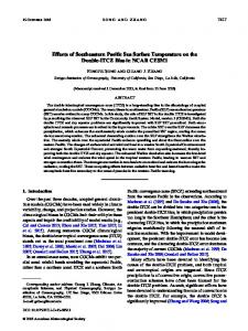
Figure 1. Vertical profiles of the 20 year averaged mean Tc5 mixing ratio (kg/kg) in control run R0. Different lines represent different latitude bands as indicated in the legend. lations were run for 23 years with the first 3 years excluded to account for model spin‐up. [8] The age tracers configured in four experiments are also listed in Table 1. In control run R0, four passive tracers had an arbitrary value of 1 kg/kg in the source region during the first month of the simulation and were then set to zero afterward (hereafter, this kind of tracer is called an age tracer). The four age tracers were released in the model at 1 hPa (Ta1), 50 hPa (Ta2), 100 hPa (Ta3) and at the model’s surface (Ta4), with same latitude range of 90°S to 90°N. A fifth passive tracer (Tc5) was released at 1 hPa with a constant value of 0.5 kg/kg in the source region during the 23 year run. The model’s surface is considered as the Tc5 sink with the surface concentrations set to zero at each time step. The passive tracer, Tc5, can be interpreted as a long‐ lived chemical tracer in stratosphere which can be absorbed at surface. With the help of tracer Tc5 we quantitatively diagnose STT properties between the upper stratosphere and the troposphere. In runs R1, R2 and R3, two age tracers are included with one being released at 1 hPa (Ta1) and the other being released at the model’s surface (Ta4).

3. Results 3.1. Overall Characteristics of Tracer Transport [9] Figure 1 shows the mean mixing ratios of Tc5 at different altitudes and latitudes during 20 years of simulation (i.e., after 3 year spin‐up) in control run R0. Average mixing ratios above 200 hPa exhibit large variations between different latitudes, reflecting regions with different stratospheric downwelling and suggesting large variations in the STT. Tc5 concentrations in the stratosphere increase with height. The lowest stratospheric concentrations are found in the tropics and the highest at southern high latitudes. Tc5 concentrations in northern high latitudes are lower than those in southern high latitudes, possibly because the southern polar vortex is stronger and persists longer than

in the north [e.g., Manney and Zurek, 1993] and the STE in the Northern Hemisphere is faster than that in the south. In the troposphere, Tc5 is well mixed and differences in its concentrations between different latitudes are small. [10] Figure 2 shows the time variation of Tc5 in control run R0 averaged at different latitude bands on three different levels. Consistent with Figure 1, Tc5 concentrations are lowest in the tropics and highest at southern high latitudes with evident latitudinal and seasonal variations at all three levels. Near the Earth’s surface, i.e., 970 hPa (Figure 2a), Tc5 concentrations are lowest in November–December at all latitudes. However, the time when Tc5 concentrations reach a maximum is different in different latitude bands. In the southern midlatitudes to high latitudes, Tc5 concentrations reach their maxima in March–April while in the northern midlatitudes and high latitudes, Tc5 concentrations are highest in June and August, respectively. In the tropics, Tc5 concentrations have their maxima in May. [11] At 50 hPa and 100 hPa, Tc5 concentrations in the Southern Hemisphere are overall out of phase with those in the north because of the seasonal shift of the meridional circulation. Tc5 concentrations are higher in the winter hemisphere than in other seasons because of accumulation of Tc5 by descent from above within the winter polar vortex [Abrams et al., 1996a, 1996b]. After spring, the polar vortex begins to break down, the strong mixing between vortex air and that from midlatitude causes a rapid decrease of Tc5 concentrations until the vortex begins to set up again after autumn. [12] It is interesting that the interannual variability of Tc5 in the southern polar vortex at 100 hPa is larger than at 50 hPa (Figures 2b and 2c). The time variation of Tc5 at high latitude at 50 hPa is more related to the polar vortex isolation and duration while at 100 hPa, which is near the tropopause region, the time variation of Tc5 is also affected by the STE processes which are more variable and irregular in time.

3 of 14

D02124


D02124

Figure 2. Time evolution of the horizontally averaged Tc5 mixing ratio (kg/kg) at (a) 970 hPa, (b) 100 hPa, and (c) 50 hPa during the 20 year integration of control run R0. Lines with different colors represent different latitude bands as marked at the bottom of the plot. [13] Having discussed the vertical distribution of Tc5 concentrations, Figure 3 further shows the horizontal distributions of the 20 year averaged Tc5 concentrations at three different levels. Near the model surface (∼970 hPa) Tc5 concentrations in the southern polar cap (which has high orography) are the largest, while lowest concentrations occur in the northern polar cap and tropics. At midlatitudes, a belt of relatively high Tc5 concentrations is found in both hemispheres at around 45° with much higher Tc5 found at regions with high landmasses, i.e., Tibetan Plateau and Rocky Mountains. Previous studies have pointed out that tropopause fold events, which are thought to be the primary process responsible for the transport of air from the stratosphere to the troposphere in midlatitudes [e.g., Andrews et al., 1987], occur frequently over elevated land surfaces [e.g., Liu et al., 1987; Austin and Midgley, 1994]. Fu et al. [2006] found, from satellite observations, that the Tibetan Plateau provides a main pathway for the STE in this region and argued that the Asian monsoon and the frequent con-

vective activities over TP are responsible for the enhanced STE. The higher Tc5 concentrations over high landmasses are possibly due to the stronger STE over those regions. On the other hand, the near‐surface model data is on a sigma surface so that Tc5 concentrations over those high landmasses will be enhanced because of the elevated surface. At 100 hPa and 50 hPa the latitudinal variations of Tc5 are similar, with Tc5 concentrations at southern high latitudes being about twice as large as those in the northern high latitudes. [14] More details of the localized downward tracer transport in the model can be obtained from the relative rate of change of Tc5 which is defined as Rt ðt2 Þ ¼ ½Cðt2 Þ Cðt1 Þ=Cðt2 Þ

where t1, t2 are two successive time steps and C is the Tc5 mixing ratio. We can infer from Rt the trend and speed of local tracer transport. Negative Rt indicates that local tracer

4 of 14

D02124


Figure 3. Horizontal distributions of the Tc5 mixing ratio (kg/kg) at (a) 970 hPa, (b) 100 hPa, and (c) 50 hPa from control run R0. Data shown are 20 year averaged climatologies.

concentrations decrease and positive Rt indicates an increase, while the value of Rt denotes the rate of change for Tc5 concentrations. Figure 4 shows the seasonal and vertical distributions of Rt in control run R0. On the global average (Figure 4a), the quickest tropospheric increase of Tc5, implying quickest STT, occurs in northern winter. Tc5 concentrations increase near the tropopause region, i.e., at around 100 hPa during April–July while from August to October Tc5 concentrations in the troposphere decrease. [15] In the tropics (Figure 4b), the Tc5 concentrations decrease from January in the upper stratosphere (negative Rt) and the regions with negative Rt propagate downward. However, the local tracer concentrations in the upper stratosphere appear to increase from April and the regions with positive Rt propagate downward until December; from June the tracer concentrations in the upper stratosphere decrease again. Note that downward propagating Rt anomalies from the upper stratosphere seem to stop descending at around 10 hPa. In the tropics, the tracer transport is determined by upwelling, also affected by horizontal mixing in upper stratosphere. Therefore, in the tropical upper stratosphere, the local positive/negative Rt implies

D02124

either that the downward transport of Tc5 from that region is weak/strong or that the horizontal transport of Tc5‐rich air from midlatitudes to tropical is strong/weak. Tc5 concentrations at around 100 hPa increase (positive Rt) from April to August. Similar positive Rt can be noted in December–February. Previous studies [e.g., Gettelman et al., 2009] showed that the tropical tropopause is highest from June–August implying the strongest tropical convective activity. The modeled vertical velocities also indicate that there is evident upward motion at around 100 hPa in the tropics during boreal summer (not shown). Therefore, Tc5 concentrations at ∼100 hPa increase (positive Rt) from April to August, possibly because of stronger convection which tends to recirculate air from below and depress the downward cross‐tropopause movement of Tc5. It is worth noting that the global mean Tc5 variations are in phase with Tc5 variations in tropics. [16] There are evident hemispheric differences in tracer transport properties at midlatitudes. At southern midlatitudes (Figure 4c), the tracer transport is characterized by a continuous downward propagation of the negative Rt regions from the upper stratosphere accompanied by a downward propagation of the positive Rt regions. In the northern midlatitude stratosphere (Figure 4d), there is a downward propagation of the positive anomalous Rt from November to April, while in other seasons, the downward propagation of anomalous Rt from the upper stratosphere is not evident. Local tracer transport is characterized by evident negative Rt (decreasing Tc5) in summer and positive Rt (increasing Tc5) in winter throughout the stratosphere. [17] At southern high latitudes (Figure 4e), Tc5 concentrations in winter increase continuously (positive Rt) in the middle and upper stratosphere because of the isolation of the vortex and strong descent within it from the Tc5 source at 1 hPa. Consequently, Tc5 concentrations below 100 hPa increase with a large positive Rt. During other times of the year, Tc5 concentrations in the southern polar stratosphere decrease overall because of horizontal exchange and mixing of air. A similar feature can be noted at northern high latitudes but out of phase with that in the south (Figure 4f). Note that tracer transport characteristics in Figures 4d and 4f are overall consistent with the results of Appenzeller et al. [1996] which showed that net cross‐tropopause mass transport in the Northern Hemisphere reaches a maximum in late spring and a distinct minimum in Autumn. 3.2. Overall Characteristics of the Mean Age‐of‐Air [18] A more quantitative measure of the STT can be seen in Figure 5 which shows the mean age‐of‐air in control run R0. The stratospheric mean (hereafter SM) age‐of‐air, derived from age tracer Ta4 released at the surface, increases above the tropopause and peaks at about 4.2 years near the stratopause (Figure 5a). This value is in accordance with the stratospheric mean age‐of‐air obtained by Garcia et al. [2007]. Compared with the results in previous SM age‐of‐ air simulations [e.g., Hall et al., 1999; Waugh and Hall, 2002], the values in Figure 4a have similar isopleths to other models, but values are slightly younger than observations presented by Waugh and Hall [2002]. Note also, unlike results of Waugh and Hall [2002], the mean age‐of‐ air is not zero at 100 hPa in the tropics since the age tracer is released at the model’s surface and the approximate value of

5 of 14

D02124


D02124

Figure 4. Seasonal variations of the Tc5 rate of change, Rt (see text for details), from control run R0 at different latitude bands. The data plotted are the 20 year averaged climatologies of Rt.

the mean age‐of‐air at around 100 hPa in tropics is about 0.3 years in our simulation. [19] When an age tracer is initially released near the stratopause (Ta1), the tropospheric mean (hereafter TM) age‐of‐air decreases with height (Figure 5d). The TM age‐ of‐air reaches 13 years in the troposphere and is much larger than the maximum SM age‐of‐air derived from the age tracer released in the troposphere. The differences between the TM and SM age‐of‐air are likely due to different characteristics for downward and upward cross‐tropopause transport processes. Exchange from troposphere to stratosphere will be preferentially in the tropics where the exchange of air across the tropopause is relatively rapid, so the SM age‐of‐air is young in the tropics. The transport from stratosphere to troposphere will occur primarily in the extratropics where transport across the tropopause occurs in both directions on time scales of a few days [Stohl et al., 2003]. Therefore, it is not the difference in time scales of the cross‐tropopause transport that cause the difference in the age‐of‐air between Figures 5a and 5d. Transport of air from the upper stratosphere to the extratropical tropopause

takes longer than transport in the other direction because of the reversed density gradient, so the TM age‐of‐air in Figure 5d is larger than the SM age‐of‐air in Figure 5a. [20] In the long‐term mean the air entering the stratosphere from the troposphere should be balanced by the air masses entering the troposphere from the stratosphere. The results discussed above suggest that downward transport from the stratosphere to the troposphere tends to occur at wider spatial scales than the upward cross‐tropopause transport to maintain mass conservation. In general, upward cross‐tropopause transport is dominated by the tropical upwelling, while downward cross tropopause transport is not only related to the large‐scale BD circulation but also related to local mesoscale processes, such as tropopause fold events, and descent within the polar vortex as well as isentropic mixing. Namely, the asymmetry of global and localized circulations, which takes in air from below at a specific region, but deposits it below at wider places, plays a role in maintaining mass conservation between the troposphere and the stratosphere. Previous studies have shown that the tropopause fold is the primary process responsible for the transport of air from the strato-

6 of 14

D02124


D02124

Figure 5. Mean age‐of‐air (years) in control run R0 derived from the age tracer released at (a) the bottom model level, (b) 100 hPa, (c) 50 hPa, and (d) 1 hPa. sphere to the troposphere in midlatitudes [e.g., Andrews et al., 1987]. Gettelman et al. [1997] pointed out that horizontal mixing of extratropical air into the tropical atmosphere is important in maintaining a global balance of STE and a more reasonable estimate of downward ozone flux from stratosphere and troposphere. [21] In the troposphere, the TM age‐of‐air in the Southern Hemisphere is older than in the north, i.e., the age tracer in the northern high latitudes is transported down to the surface faster than at southern high latitudes because of stronger and more frequent synoptic events in the north. Figures 2 and 3 show that the tropospheric Tc5 is largest in the Southern Hemisphere, also implying that Tc5 remained in the atmosphere longer and maintained to higher concentrations. [22] When the age tracer is initially released at 100 hPa (Ta3) and 50 hPa (Ta2), the SM age‐of‐air in the stratosphere is about 0.7 years younger in Figure 5b and about 1.7 years younger in Figure 5c compared to Figure 5a. It seems that downward tracer transport from 100 hPa to the surface needs on the order of 3.5 years (about 9.5 years younger than in Figure 5d) but about 10 years for the tracer to travel from 50 hPa to the surface (about 3 years younger than that in Figure 5d). Figures 5b and 5c also indicate that the mean tropospheric age‐of‐air is younger in the Northern Hemisphere, which is consistent with Figure 5d.

3.3. Effects of SST and GHG Changes on the Age‐of‐Air 3.3.1. Age‐of‐Air Changes [23] In this section we discuss the effect of SST and GHG changes on the mean age‐of‐air. We start the analysis by comparing the mean age‐of‐air under different configurations of SSTs and age tracers in the model. Figure 6 shows changes in the mean age‐of‐air because of 0.5–1.5 K increases in SSTs. Also shown in Figure 6 are the mean age differences between control run R0 and run R3 (with 2100 GHG and SST conditions). It should be pointed out that the mean age‐of‐air in Figure 6 is derived from the age tracer released at 1 hPa (Ta1) and the age differences can be interpreted as changes in the speed of downward tracer transport. It is evident that the TM age‐of‐air increases in broad regions of the stratosphere and decreases in the troposphere when SSTs are uniformly increased (Figures 6a and 6b). The larger SST increases give rise to a larger mean age‐of‐air in the stratosphere and a smaller mean age‐of‐air in the troposphere. It is suggested that increased SSTs tend to accelerate upward transport because of enhanced convective activity in the troposphere [Rosenlof and Reid, 2008]. Olsen et al. [2007] pointed out that increased SSTs can result in a stronger Brewer‐Dobson (BD) circulation and enhanced tropical upwelling. Stronger

7 of 14

D02124


D02124

that in control run R0. Figure 6c further confirms that the larger SST increases give rise to a larger TM age‐of‐air in the stratosphere and a smaller TM age‐of‐air in the troposphere Also note that changes in the TM age‐of‐air in the troposphere in R3 are more pronounced in the Northern Hemisphere and a decrease in mean age‐of‐air in the northern midlatitude and high latitude stratosphere is evident. [25] Analogous to Figure 6, Figure 7 shows changes of the SM age‐of‐air derived from the age tracer released at the model’s surface (Ta4). The age differences in Figure 7 can be interpreted as changes in the speed of upward tracer transport. We can see that uniform 0.5 K and 1.5 K increases in SST cause an overall decrease in the SM age‐of‐air in the stratosphere, implying that SST increases lead to quicker upward transport (Figures 7a and 7b). This result coincides with a previous study [García‐Herrera et al., 2006]. The changes in the SM age‐of‐air in the stratosphere are not proportional to the SST increases. A uniform 0.5 K increase in SSTs causes a 0.10–0.25 year decrease in the SM age‐of‐ air in the stratosphere, while a 1.5 K SST increase causes a 0.20–0.40 year decrease. In run R3, the SM age‐of‐air in the

Figure 6. Differences (months) in the mean age‐of‐air between (a) control run R0 and run R1, (b) control run R0 and run R2, and (c) control run R0 and run R3. The mean age‐of‐air is derived from the age tracer released at 1 hPa (Ta1). and more frequent convection implies a quicker transport of air masses below the tropopause, and consequently, the TM age‐of‐air decreases when SSTs are increased. In the stratosphere, the TM age‐of‐air increases should be also related to the intensified BD circulation, which accelerates upward transport and, accordingly, slows downward transport in broad regions of lower‐latitude stratosphere. For an age tracer moving from troposphere to stratosphere it will enter the tropical tropopause region and be carried quickly upward. It can then descend slowly, but since that descent is over a larger region (outside the tropical pipe) the descent velocity can be slower. This balances the mass flux of air across the tropopause, but the slower descent leads to higher age for the stratopause age tracer. [24] When the SST and GHG values are both changed to match 2100 conditions, the changes in TM age‐of‐air (Figure 6c) are slightly larger than those in Figure 6b. Recall that the global‐mean SST in run R3 is about 2.0 K higher than

Figure 7. As Figure 6 but for results derived from the age tracer released at the bottom model level (Ta4).

8 of 14

D02124


Figure 8. Temperature differences (K) between (a) runs R0 and R1, (b) runs R0 and R2, and (c) runs R0 and R3. The temperatures are 20 year averaged climatologies. Shaded regions denote differences that are statistically significant at the 95% level. Solid lines represent positive contours, and dashed lines represent negative contours. stratosphere is much younger with a maximum decrease of 0.8 years in the southern upper stratosphere and northern lower stratosphere relative to control run R0 (Figure 7c). This result indicates that changes in the SM age‐of‐air caused by the SST changes alone are not as large as GHG changes. Without changes in GHG values, in run R2 the decrease of the SM age‐of‐air caused by SST changes is about one half of that caused by the combined SST and GHG changes. [26] Previous modeling studies have also found that the SM age‐of‐air in the stratosphere becomes younger in the future climate because of the strengthened BD circulation and tropical upwelling [e.g., Austin et al., 2007; Garcia and Randel, 2008]. It is interesting that changes in the TM age‐ of‐air derived from the age tracer released at 1 hPa (Figures 6) are larger in magnitude than changes in the SM age‐of‐air derived from the age tracer released at the model’s surface (Figure 7). However, the differences between increases in TM age‐of‐air in the stratosphere because of different SST and GHG changes are relatively smaller than the differences

D02124

between decreases in the SM age‐of‐air in the stratosphere caused by different SST and GHG changes. 3.3.2. Dynamical Responses [27] Figure 8 gives the zonal mean temperature differences between control run R0 and runs R1, R2 and R3. The temperature changes caused by a uniform 1.5 K SST increase have a similar spatial pattern as the temperature changes caused by a uniform 0.5 K SST increase. A uniform 0.5 K/1.5 K increase in SSTs warms the troposphere but cools the tropical stratosphere with a maximum warming of 0.8 K/2.5 K in the middle troposphere and a maximum cooling of 0.3 K/0.6 K in the tropical upper stratosphere. Note that SSTs increases in run R1 and R2 cause a warming of the polar stratosphere. Garfinkel and Hartman [2007] also found that SST changes have a significant effect on stratospheric temperatures in winter. [28] It is apparent that the stratospheric responses to SST and GHG increases are quite different. Compared to temperature changes because of a uniform 1.5 K increase in SSTs, the warming of the troposphere and the cooling of the stratosphere because of combined effects of SST and GHG increases are more pronounced and uniform (Figure 8c), with a maximum 3 K warming in the troposphere and a 15 K cooling in the upper stratosphere. The results in Figure 8c are also qualitatively similar to those of Kodama et al. [2007] and Xie et al. [2008]. Note that the 15 K cooling in the upper stratosphere, which seems very large, is an absolute difference, not the temperature trend. If we roughly estimate a trend relative to control run, we get a temperature trend of around −1.4 K/decade at 1 hPa, which is larger than −1.0 K/decade obtained by Eyring et al. [2007]. Note that this trend is estimated from two time slice runs for 2000 and 2100 SST and GHG conditions, respectively, while the trend of Eyring et al. [2007] was derived from temperature time series of transient CCM runs. Uncertainties may exist in the temperature trend estimated from time slice runs. [29] The vertical propagation of planetary waves from the troposphere into the stratosphere plays a significant role in determining temperatures of the stratosphere [e.g., Hardiman et al., 2007]. The wave forcing can be quantified in terms of the meridional heat flux v′T ′ at 100 hPa [e.g., Eyring et al., 2006], which is proportional to the vertical flux of wave activity via the Eliassen‐Palm (EP) wave flux, and the polar cap averaged temperatures are well correlated with the meridional heat flux at 100 hPa [Newman et al., 2001]. Table 2 lists the time‐mean meridional heat fluxes at 100 hPa for both hemisphere winters averaged from 40°– 80° in the four different runs. Compared to the heat flux in Table 2. Time‐Mean Meridional Horizontal Eddy Heat Flux v′T ′ (K m/s) at 100 hPa Averaged Over 40°N–80°N for December, January, February and Averaged Over 40°S–80°S for June, July, Augusta Experiment

v′T ′ (Northern Hemisphere)

v′T ′ (Southern Hemisphere)

R0 R1 R2 R3

8.286 7.999 (−0.287) 7.107 (−1.179) 7.347 (−0.939)

5.459 5.600 (0.141) 5.507 (0.048) 4.542 (−0.917)b

a Values in parentheses indicate the differences between the corresponding run and control run. b Differences that are statistically significant at the 95% level.

9 of 14

D02124


D02124

Figure 9. (a) Annual mean Eliasen‐Palm (EP) flux (kg s−2) vectors from control run R0. The differential EP flux vectors between (b) runs R1 and R0, (c) runs R2 and R0, and (d) runs R3 and R0. The unit vectors are shown to the right of each panel. Note that the vertical unit vectors are different among runs R1, R2, and R3. control run R0, 0.5–1.5 K SST increases in run R1 and R2 cause an increase in meridional heat flux at 100 hPa in the Southern Hemisphere high latitude but a decrease in Northern Hemisphere high latitude. However, the changes in the heat flux in run R1 and R2 are not statistically significant. [30] When both SST and GHG values are increased, the meridional heat flux for the boreal winter decreases. The results here suggest that the responses of the polar stratosphere to SST and GHG increases are different, i.e., SST increases tend to increase the meridional heat flux in the southern high‐latitude stratosphere while GHG increases are likely to decrease it because of the significant cooling of the stratosphere caused by GHG increases. With significant cooling of stratosphere in R3, the vortex is strengthened and planetary wave amplitudes tend to be reduced and the heat flux decreases. In addition, as the polar stratospheric temperature is determined by both radiative and dynamical processes, although the wave forcing change can partly

contribute to the stratospheric temperature changes, the cooling of the stratosphere in run R3 is mainly due to increased GHGs. Garny et al. [2009] pointed out that trends in stratospheric temperature are largely driven by changes in concentrations of GHGs, and that changes in SST have a secondary impact. Li et al. [2008] also pointed out that the polar stratospheric temperature is, in general, determined both by radiation and dynamical processes with radiative processes being dominant in driving the long‐term variations of the Antarctic lower‐stratospheric temperature in Southern Hemisphere spring and summer. [31] Figure 9 further shows anomalous EP flux vectors caused by SST and GHG changes. In the high‐latitude stratosphere, an uniform 0.5–1.5 K SST increase causes an increase in the EP flux in the Southern Hemisphere, but a decrease in the Northern Hemisphere (Figures 9b and 9c). However, when both SST and GHG values are increased in run R3, the EP flux at high latitudes weakens in both hemisphere stratosphere (Figure 9d). It is apparent that EP

10 of 14

D02124


D02124

Figure 10. Differences in stratospheric water vapor (ppmm) between (a) control run R0 and run R2 and (b) control run R0 and run R3. Shaded regions denote differences that are statistically significant at the 95% level. Solid lines represent positive contours, and dashed lines represent negative contours with intervals of 0.05 ppmm. flux changes in the lower latitudes are different from those in the high‐latitude stratosphere. The EP flux strengthens over broad regions of the subtropics and tropics and northern midlatitudes. Previous studies have shown that changes in wave driving at lower latitudes (20°–40°) must be responsible for the BD circulation changes [Fomichev et al., 2007; Butchart et al., 2006], while Garcia and Randel [2008] concluded that the BD circulation strengthened as a result of enhanced EP flux in subtropics even if EP flux was suppressed in midlatitudes and high latitudes. The analysis of the residual circulation reveals that w* at 100 hPa averaged over 30°S–30°N in run R1 and R2 is 2% and 7.7% larger than that in control run R0. [32] It is interesting that when both SST and GHG values are increased in run R3, the enhancement of the upward EP flux is much larger in the lower latitudes compared with those in runs R0, R1 and R2, while downward EP flux is strengthened over the high latitudes stratosphere (Figure 9d). w* at 100 hPa averaged over the tropics increases by about 15% compared to that in run R0. The analysis above suggests that combined effects of GHG and SST changes can cause more evident changes in BD circulation (Figure 9), the SM age‐of‐air (Figure 7) than those caused by SST changes alone. Similar results have been

obtained in previous studies [e.g., Li et al., 2008; Xie et al., 2008]. The GHG increase in run R3 causes troposphere warming and stratosphere cooling (Figure 8c), leading to an enhanced meridional temperature gradient in the upper troposphere and lower stratosphere (UTLS). The increased meridional temperature gradient results in enhanced planetary wave propagation into the stratosphere [e.g., Eichelberger and Hartmann, 2005], which makes a primary contribution to the intensification of the BD circulation [e.g., Haynes et al., 1991]. 3.4. Effect of SST and GHG Changes on Stratospheric H2O [33] We now examine the stratospheric water vapor changes induced by changes in SSTs and GHGs. Figure 10 gives stratospheric water vapor differences between run R2 and R0, and between R3 and R0. A uniform 1.5 K SST increase causes an overall increase of water vapor throughout the stratosphere (Figure 10a). Under the 2100 SST and GHG conditions, the stratospheric water vapor increases more significantly over the stratosphere (Figure 10b) with a different spatial pattern from that in Figure 10a. The stratospheric water vapor increases because of a 1.5 K increase in SSTs are about 0.2–0.3 ppmv and relatively uniform in space.

11 of 14

D02124


Figure 11. (a) Seasonal variation of the tropical cold point tropopause temperature (averaged between 30°N–30°S) in four model runs. (b) Correlations between 100 hPa temperature and the water vapor (solid line) in the tropical lower stratosphere (averaged from 100 hPa to 70 hPa between 30°S–30°N) and (dash‐dotted line) in the tropical upper stratosphere (averaged from 70 hPa to 10 hPa). Under the 2100 SST and GHG condition, GHG increases affect stratospheric water vapor not only by changing the tropopause temperature and transport properties, but also via methane oxidation. Consequently, the stratospheric water vapor increases under the 2100 SST and GHG condition have evident spatial variations with maximum increases occur in the upper stratosphere at high latitudes. An exception is found in the Southern Hemisphere polar stratosphere in Figure 10b, where water vapor is slightly decreased in run R3 despite significant water vapor increases elsewhere. According to Garcia et al. [2007], this water vapor anomaly is possibly due to the dehydration process associated with noticeably low temperatures in the polar vortex. We can see from Figure 8c that the temperatures near 100 hPa at southern high latitudes in run R3 are about 3 K lower than those in run R0, but are about the same between runs R2 and R0 (Figure 8b). Therefore, the dehydration is more likely in run R3 than in R2. [34] The water vapor increases in the northern high latitudes lower stratosphere in run R2 and R3 are larger than those in the southern lower stratosphere, implying that STE in the Northern Hemisphere is stronger than that in the Southern Hemisphere. Another possible reason is more air

D02124

circulates to the north than to the south. This result is consistent with the transport characteristics of age tracers which indicate that SM mean age‐of‐air in the Southern Hemisphere is older than that in the Northern Hemisphere. It is worth noting that the transport of a passive tracer and water vapor between the troposphere and the stratosphere is different. The water vapor entering into the stratosphere is mainly controlled by the tropopause temperature if the chemical contribution from the methane oxidation is excluded. [e.g., Tian and Chipperfield, 2006], but the tracer transport between the troposphere and stratosphere is solely determined by the dynamical processes. [35] Figure 11a gives seasonal variations of the tropical cold point tropopause temperature (averaged between 30°N–30°S) in the four runs. We can see that the tropical cold point tropopause temperature increases as the SST increases. However, the cold point tropopause temperature in run R3 is not the warmest among the four runs, although the global mean SSTs in R3 is about 2.0 K higher than that in control run R0. It is possible that the tropical cold point tropopause temperature in run R3 is suppressed by the adiabatic cooling associated with enhanced tropical upwelling (15% increase in w* at 100 hPa in tropics) [Zhou et al., 2001] and the stratospheric cooling caused by increased GHGs values. Although the cold point tropopause temperature is not the warmest, the stratospheric water vapor in run R3 is the largest (Figure 10) because of the enhanced methane oxidation and tropical upwelling under 2100 conditions. In addition, the cold point tropopause temperature in run R3 is evidently higher than that in run R0 during March to August, but in other months, the differences in tropical cold point tropopause temperatures between run R0 and run R3 are small. Gettelman et al. [2010] found that most chemistry‐ climate model simulations do not produce strong long‐term trends in annual mean tropical cold point tropopause temperature. Figure 11a suggests that responses of tropical cold point tropopause temperature to SST and GHG increases are seasonal‐dependent. [36] Figure 11b further shows that the correlation between the stratospheric water vapor and 100 hPa temperature is nearly linear with a 1 K increase in 100 hPa temperature corresponding a 0.377 ppmm water vapor increase in the tropical lower stratosphere (100–70 hPa) and a 0.290 ppmm increase in the tropical upper stratosphere (70–10 hPa). Note that under the 2100 SST and GHG conditions, stratospheric water vapor changes are partly caused by the methane oxidation, therefore the corresponding data from run R3 is excluded in Figure 11b. It is worth pointing out that an anticorrelation also exists between the stratospheric water vapor and the SM age‐of‐air, but to establish a causal relation between them is not straightforward.

4. Conclusion and Discussion [37] We have investigated the transport characteristics between the stratosphere and troposphere using a state‐of‐ the‐art GCM. There are significant hemispheric differences in tracer transport properties at midlatitudes and high latitudes. The downward tracer transport in the northern midlatitude stratosphere is faster than at southern midlatitudes, whereas the descent is stronger in the southern polar region than in the north. On the global average (Figure 4a), the

12 of 14

D02124


fastest increase of the stratospheric source tracer (Tc5) in the troposphere, implying that most rapid STT occurs in northern winter. Tc5 concentrations increase near the tropopause region during April–July while from August to October Tc5 concentrations in the troposphere decrease, suggesting that the downward transport of Tc5 is weakest during this period. [38] The maximum troposphere mean age‐of‐air derived from an age tracer released in the upper stratosphere can reach 13 years and is much larger than the maximum stratosphere mean age‐of‐air derived from the age tracer released from the troposphere, suggesting that tracer transport from the troposphere to stratosphere is more rapid than from the stratosphere to troposphere. The TM age‐of‐air in the Southern Hemisphere is older than in the Northern Hemisphere, i.e., the age tracer in the northern midlatitudes and high latitudes is transported down to the surface faster than in the southern midlatitude and high latitude because of stronger and more frequent synoptic events in the Northern Hemisphere. [39] In the stratosphere, increased SSTs tend to accelerate upward transport because of enhanced upwelling from the troposphere. Changes in the SM age‐of‐air caused by uniform increases in SSTs are much smaller than those caused by the combined changes in SSTs and GHG values. Increased SSTs tends to slow the downward transport in the stratosphere and cause increases in the TM age‐of‐air. The larger SST increases give rise to a larger TM age‐of‐air in the stratosphere and a smaller TM age‐of‐air in the troposphere. Changes in the TM age‐of‐air caused by increased SSTs are larger in magnitude than corresponding changes in the SM age‐of‐air. However, the differences between increases in TM age‐of‐air in the stratosphere because of different SST and GHG increases are smaller than the differences between decreases in the SM age‐of‐air in the stratosphere caused by different SST and GHG increases. [40] An increase in SSTs enhances the extratropical upward Eliasen‐Palm flux and the tropical upwelling, with a significant 7.7% enhancement in tropical upwelling caused by a uniform 1.5 K SST increase. Uniform SST increases cause an increase in meridional heat flux at 100 hPa in the Southern Hemisphere high latitude but a decrease in Northern Hemisphere high latitude. When both SST and GHG values are increased, the meridional heat flux decreases in both winter hemispheres, although the EP flux increases significantly in broad regions of extratropics and leads to a 15% enhancement in tropical upwelling. The responses of polar stratosphere to SST and GHG increases are different. SST increases tend to increase the meridional heat flux in the southern high‐latitude stratosphere, while GHG increases are likely to decrease it because of the significant stratospheric cooling caused by GHG increases. [41] Acknowledgments. This work was supported by the National Science Foundation of China (40730949) and National Basic Research Program of China (2010CB428604). W.T. also thanks the New Century Young Scientist Support Project and Doctoral Funds of Education Ministry of China. We thank Dan Marsh for providing the WACCM model and the Gansu Computing Center for computing support. We thank three anonymous reviewers for their helpful comments which improve the paper substantially. We thank R. Garcia, A. Gettelman, and D. Kinnison for supplying the WACCM ozone data for 2090–2099 and SPARC CCMval project for providing SST and sea ice fields.

D02124

References Abrams, M. C., et al. (1996a), ATMOS/ATLAS‐3 observations of long‐ lived tracers and descent in the Antarctic vortex in November 1994, Geophys. Res. Lett., 23(17), 2341–2344, doi:10.1029/96GL00705. Abrams, M. C., et al. (1996b), Trace gas transport in the Arctic vortex inferred from ATMOS ATLAS‐2 observations during April 1993, Geophys. Res. Lett., 23(17), 2345–2348, doi:10.1029/96GL00704. Andrews, D. G., J. R. Holton, and C. B. Leovy (1987), Middle Atmosphere Dynamics, Academic, San Diego, Calif. Appenzeller, C., J. R. Holton, and K. H. Rosenlof (1996), Seasonal variation of mass transport across the tropopause, J. Geophys. Res., 101(D10), 15,071–15,078, doi:10.1029/96JD00821. Austin, J., and F. Li (2006), On the relationship between the strength of the Brewer‐Dobson circulation and the age of stratospheric air, Geophys. Res. Lett., 33, L17807, doi:10.1029/2006GL026867. Austin, J. F., and R. P. Midgley (1994), The climatology of the jet stream and stratospheric intrusions of ozone over Japan, Atmos. Environ., 28, 39–52, doi:10.1016/1352-2310(94)90021-3. Austin, J., J. Wilson, F. Li, and H. Vomel (2007), Evolution of water vapor concentrations and stratospheric age of air in coupled chemistry‐climate model simulations, J. Atmos. Sci., 64, 905–921, doi:10.1175/JAS3866.1. Austin, J., et al. (2010), Decline and recovery of total column ozone using a multimodel time series analysis, J. Geophys. Res., 115, D00M10, doi:10.1029/2010JD013857. Butchart, N., and A. A. Scaife (2001), Removal of chlorofluorocarbons by increased mass exchange between the stratosphere and the troposphere in a changing climate, Nature, 410, 799–802, doi:10.1038/35071047. Butchart, N., et al. (2006), Simulations of anthropogenic change in the strength of the Brewer‐Dobson circulation, Clim. Dyn., 27, 727–741, doi:10.1007/s00382-006-0162-4. Collins, W. J., R. G. Derwent, B. Garnier, C. E. Johnson, M. G. Sanderson, and D. S. Stevenson (2003), Effect of stratosphere‐troposphere exchange on the future tropospheric ozone trend, J. Geophys. Res., 108(D12), 8528, doi:10.1029/2002JD002617. Eichelberger, S. J., and D. L. Hartmann (2005), Changes in the strength of the Brewer‐Dobson circulation in a simple AGCM, Geophys. Res. Lett., 32, L15807, doi:10.1029/2005GL022924. Engel, A., et al. (2009), Age of stratospheric air unchanged within uncertainties over the past 30 years, Nature, 2, 28–31, doi:10.1038/ngeo388. Eyring, V., et al. (2006), Assessment of temperature, trace species, and ozone in chemistry‐climate model simulations of the recent past, J. Geophys. Res., 111, D22308, doi:10.1029/2006JD007327. Eyring, V., et al. (2007), Multimodel projections of ozone recovery in the 21st century, J. Geophys. Res., 112, D16303, doi:10.1029/2006JD008332. Eyring, V., et al. (2008), Overview of the new CCMVal reference and sensitivity simulations in support of upcoming ozone and climate assessments and planned SPARC CCMVal, SPARC Newsl., 30, 20–26. Fomichev, V. I., A. I. Jonsson, J. de Grandpré, S. R. Beagley, C. McLandress, K. Semeniuk, and T. G. Shepherd (2007), Response of the middle atmosphere to CO2 doubling: Results from the Canadian Middle Atmosphere Model, J. Clim., 20, 1121–1144, doi:10.1175/JCLI4030.1. Fu, R., et al. (2006), Short circuit of water vapor and polluted air to the global stratosphere by convective transport over the Tibetan Plateau, Proc. Natl. Acad. Sci. U. S. A., 103, 5664–5669, doi:10.1073/pnas.0601584103. Garcia, R. R., and W. J. Randel (2008), Acceleration of the Brewer‐Dobson circulation due to increases in greenhouse gases, J. Atmos. Sci., 65, 2731–2739. doi:10.1175/2008JAS2712.1. Garcia, R. R., D. R. Marsh, D. E. Kinnison, B. A. Boville, and F. Sassi (2007), Simulation of secular trends in the middle atmosphere, 1950–2003, J. Geophys. Res., 112, D09301, doi:10.1029/2006JD007485. García‐Herrera, R., N. Calvo, R. R. Garcia, and M. A. Giorgetta (2006), Propagation of ENSO temperature signals into the middle atmosphere: A comparison of two general circulation models and ERA‐40 reanalysis data, J. Geophys. Res., 111, D06101, doi:10.1029/2005JD006061. Garfinkel, C. I., and D. L. Hartmann (2007), Effects of the El Nino–Southern Oscillation and the Quasi‐Biennial Oscillation on polar temperatures in the stratosphere, J. Geophys. Res., 112, D19112, doi:10.1029/2007JD008481. Garny, H., M. Dameris, and A. Stenke (2009), Impact of prescribed SSTs on climatologies and long‐term trends in CCM simulations, Atmos. Chem. Phys., 9, 6017–6031, doi:10.5194/acp-9-6017-2009. Gerber, E. P., et al. (2010), Stratosphere‐troposphere coupling and annular mode variability in chemistry‐climate models, J. Geophys. Res., 115, D00M06, doi:10.1029/2009JD013770. Gettelman, A., J. R. Holton, and K. H. Rosenlof (1997), Mass fluxes of O3, CH4, N2O and CF2Cl2 in the lower stratosphere calculated from observational data, J. Geophys. Res., 102(D15), 19,149–19,159, doi:10.1029/ 97JD01014. Gettelman, A., et al. (2009), The tropical tropopause layer 1960–2100, Atmos. Chem. Phys., 9, 1621–1637, doi:10.5194/acp-9-1621-2009.

13 of 14

D02124


Gettelman, A., et al. (2010), Multimodel assessment of the upper troposphere and lower stratosphere: Tropics and global trends, J. Geophys. Res., 115, D00M08, doi:10.1029/2009JD013638. Hall, T. M., D. W. Waugh, K. A. Boering, and R. A. Plumb (1999), Evaluation of transport in stratospheric models, J. Geophys. Res., 104(D15), 18,815–18,839, doi:10.1029/1999JD900226. Hardiman, S. C., N. Butchart, P. H. Haynes, and S. H. E. Hare (2007), A note on forced versus internal variability of the stratosphere, Geophys. Res. Lett., 34, L12803, doi:10.1029/2007GL029726. Haynes, P. H., M. E. McIntyre, T. G. Shepherd, C. J. Marks, and K. P. Shine (1991), On the “downward control” principle of extratropical circulations by eddy‐induced mean zonal forces, J. Atmos. Sci., 48, 651–678, doi:10.1175/1520-0469(1991)0482.0.CO;2. Hegglin, M. I., et al. (2010), Multimodel assessment of the upper troposphere and lower stratosphere: Extratropics, J. Geophys. Res., 115, D00M09, doi:10.1029/2010JD013884. Holton, J. R., P. H. Haynes, M. E. McIntyre, A. R. Douglass, R. B. Rood, and L. Pfister (1995), Stratosphere‐troposphere exchange, Rev. Geophys., 33(4), 403–439, doi:10.1029/95RG02097. Kodama, C., T. Iwasaki, K. Shibata, and S. Yukimoto (2007), Changes in the stratospheric mean meridional circulation due to increased CO2: Radiation‐ and sea surface temperature–induced effects, J. Geophys. Res., 112, D16103, doi:10.1029/2006JD008219. Li, F., J. Austin, and J. Wilson (2008), The strength of the Brewer‐Dobson circulation in a changing climate: Coupled chemistry‐climate model simulations, J. Clim., 21, 40–57, doi:10.1175/2007JCLI1663.1. Liu, S. C., M. Trainer, F. C. Fehsenfeld, D. D. Parrish, E. J. Williams, D. W. Fahey, G. Hubler, and P. C. Murphy (1987), Ozone production in the rural troposphere and the implications for regional and global ozone distributions, J. Geophys. Res., 92(D4), 4191–4207, doi:10.1029/ JD092iD04p04191. Manney, G. L., and R. W. Zurek (1993), Interhemispheric comparison of the development of the stratospheric polar vortex during fall: A 3‐dimensional perspective for 1991–1992, Geophys. Res. Lett., 20(12), 1275–1278, doi:10.1029/93GL01111. Meloen, J., et al. (2003), Stratosphere‐troposphere exchange: A model and method intercomparison, J. Geophys. Res., 108(D12), 8526, doi:10.1029/ 2002JD002274. Monge‐Sanz, B., M. P. Chipperfield, A. Simmons, and S. Uppala (2007), Mean age of air and transport in a CTM: Comparison of different ECMWF analyses, Geophys. Res. Lett., 34, L04801, doi:10.1029/2006GL028515. Morgenstern, O., et al. (2010), Review of the formulation of present‐ generation stratospheric chemistry‐climate models and associated external forcings, J. Geophys. Res., 115, D00M02, doi:10.1029/2009JD013728. Newman, P. A., E. R. Nash, and J. E. Rosenfield (2001), What controls the temperature of the Arctic stratosphere during spring?, J. Geophys. Res., 106(D17), 19,999–20,010, doi:10.1029/2000JD000061. Olsen, M. A., M. R. Schoeberl, and J. E. Nielsen (2007), Response of stratospheric circulation and stratosphere‐troposphere exchange to

D02124

changing sea surface temperatures, J. Geophys. Res., 112, D16104, doi:10.1029/2006JD008012. Rosenlof, K. H., and G. C. Reid (2008), Trends in the temperature and water vapor content of the tropical lower stratosphere: Sea surface connection, J. Geophys. Res., 113, D06107, doi:10.1029/2007JD009109. Sassi, F., R. Garcia, B. Boville, and H. Liu (2002), On temperature inversions and the mesospheric surf zone, J. Geophys. Res., 107(D19), 4380, doi:10.1029/2001JD001525. Schoeberl, M. R. (2004), Extratropical stratosphere‐troposphere mass exchange, J. Geophys. Res., 109, D13303, doi:10.1029/2004JD004525. Schoeberl, M. R., and A. R. Douglass (2005), Estimation of stratospheric age spectrum from chemical tracers, J. Geophys. Res., 110, D21303, doi:10.1029/2005JD006125. Stohl, A., et al. (2003), Stratosphere‐troposphere exchange: A review, and what we have learned from STACCATO, J. Geophys. Res., 108(D12), 8516, doi:10.1029/2002JD002490. Tian, W., and M. P. Chipperfield (2005), A new coupled chemistry‐climate model for the stratosphere: The importance of coupling for future O3‐climate predictions, Q. J. R. Meteorol. Soc., 131, 281–303, doi:10.1256/qj.04.05. Tian, W., and M. P. Chipperfield (2006), Stratospheric water vapor trends in a coupled chemistry‐climate model, Geophys. Res. Lett., 33, L06819, doi:10.1029/2005GL024675. Waugh, D. (2009), Atmospheric dynamics: The age of stratospheric air, Nature, 2, 14–16, doi:10.1038/ngeo397. Waugh, D. W., and T. M. Hall (2002), Age of stratospheric air: Theory, observations, and models, Rev. Geophys., 40(4), 1010, doi:10.1029/ 2000RG000101. Wild, O. (2007), Modeling the global tropospheric ozone budget: Exploring the variability in current models, Atmos. Chem. Phys., 7, 2643–2660, doi:10.5194/acp-7-2643-2007. World Meteorological Organization (2003), Scientific assessment of ozone depletion: 2002, Rep. 47, WMO Global Ozone Res. and Monit. Proj., Geneva, Switzerland. Xie, F., W. Tian, and M. P. Chipperfield (2008), Radiative effect of ozone change on stratosphere‐troposphere exchange, J. Geophys. Res., 113, D00B09, doi:10.1029/2008JD009829. Zhou, X.‐L., M. A. Geller, and M. Zhang (2001), Cooling trend of the tropical cold point tropopause temperatures and its implications, J. Geophys. Res., 106(D2), 1511–1522, doi:10.1029/2000JD900472. J. Austin, NOAA Geophysical Fluid Dynamics Laboratory, Princeton Forrestal Campus Rte. 1, 201 Forrestal Rd., Princeton, NJ 08542‐0308, USA. M. P. Chipperfield, ICAS, School of Earth and Environment, University of Leeds, LS2 9JT, UK. J. Shu, W. Tian, W. Wang, and F. Xie, Key Laboratory for Semi‐Arid Climate Change of the Ministry of Education, College of Atmospheric Sciences, Lanzhou University, Lanzhou, Gansu 730000, China. (wstian@ lzu.edu.cn)

14 of 14