efficiency of biomass energy

EFFICIENCY OF BIOMASS ENERGY

EFFICIENCY OF BIOMASS ENERGY An Exergy Approach to Biofuels, Power, and Biorefineries

Krzysztof J. Ptasinski

Copyright  2016 by John Wiley & Sons, Inc. All rights reserved. Published by John Wiley & Sons, Inc., Hoboken, New Jersey. Published simultaneously in Canada. No part of this publication may be reproduced, stored in a retrieval system, or transmitted in any form or by any means, electronic, mechanical, photocopying, recording, scanning, or otherwise, except as permitted under Section 107 or 108 of the 1976 United States Copyright Act, without either the prior written permission of the Publisher, or authorization through payment of the appropriate per-copy fee to the Copyright Clearance Center, Inc., 222 Rosewood Drive, Danvers, MA 01923, (978) 750-8400, fax (978) 750-4470, or on the web at www.copyright.com. Requests to the Publisher for permission should be addressed to the Permissions Department, John Wiley & Sons, Inc., 111 River Street, Hoboken, NJ 07030, (201) 748-6011, fax (201) 748-6008, or online at http://www.wiley.com/go/permission. Limit of Liability/Disclaimer of Warranty: While the publisher and author have used their best efforts in preparing this book, they make no representations or warranties with respect to the accuracy or completeness of the contents of this book and specifically disclaim any implied warranties of merchantability or fitness for a particular purpose. No warranty may be created or extended by sales representatives or written sales materials. The advice and strategies contained herein may not be suitable for your situation. You should consult with a professional where appropriate. Neither the publisher nor author shall be liable for any loss of profit or any other commercial damages, including but not limited to special, incidental, consequential, or other damages. For general information on our other products and services or for technical support, please contact our Customer Care Department within the United States at (800) 762-2974, outside the United States at (317) 572-3993 or fax (317) 572-4002. Wiley also publishes its books in a variety of electronic formats. Some content that appears in print may not be available in electronic formats. For more information about Wiley products, visit our web site at www.wiley.com. Library of Congress Cataloging-in-Publication Data is available. ISBN: 978-1-118-70210-9 Printed in the United States of America 10 9 8 7 6 5 4 3 2 1

Contents Preface xv Acknowledgments xix About the Author xxi

PART I

|

Background and Outline

Chapter 1 | Bioenergy Systems: An Overview

3

1.1

Energy and the Environment 3 1.1.1 Global Energy Consumption 3 1.1.2 Conversion and Utilization of Energy 7 1.1.3 Fossil Fuel Resources 8 1.1.4 Environmental Impact of Fossil Fuels Use 9 1.1.5 Renewable Energy 11 1.2 Biomass as a Renewable Energy Source 13 1.2.1 Introduction 13 1.2.2 Historical Development and Potential of Bioenergy 14 1.2.3 Biomass Resources 16 1.2.4 Biomass Properties 17 1.2.5 Environmental Impact of Bioenergy 19 1.2.6 Economics of Bioenergy 21 1.3 Biomass Conversion Processes 22 1.3.1 Introduction 22 1.3.2 Upgrading Technologies 23 1.3.3 Thermochemical Conversion Processes 24 1.3.4 Biochemical Conversion Processes 25 1.3.5 Chemical Conversion Processes 26 1.4 Utilization of Biomass 27 1.4.1 Introduction 27 1.4.2 Biofuels 29 1.4.3 Electric Power Generation 31 1.4.4 Heat Production 32 1.4.5 Chemical Biorefinery 33 1.5 Closing Remarks 34 References 34

Chapter 2 | Exergy Analysis 2.1

37

Sustainability and Efficiency 37 2.1.1 Sustainable Development 37 2.1.2 Sustainability Methods and Metrics 39 2.1.3 Thermodynamic Approach to Sustainability and Efficiency 40

v

vi

CONTENTS

2.2

Thermodynamic Analysis of Processes 42 2.2.1 Introduction 42 2.2.2 Mass and Energy Rate Balances for a Steady Flow Process – the First Law of Thermodynamics 42 2.2.3 Quality of Energy and Materials 43 2.2.4 Entropy and the Second Law of Thermodynamics 45 2.2.5 Entropy Production 47 2.2.6 Entropy Rate Balance for a Steady Flow Process 50 2.2.7 Maximum Work Obtainable from a Steady Flow Process 51 2.3 Exergy Concept 52 2.3.1 Defining Exergy 52 2.3.2 Exergy Reference Environment 54 2.3.3 Exergy versus Energy 55 2.3.4 Exergy of Work and Heat Transfer 56 2.3.5 Exergy of a Stream of Matter 59 2.3.6 Physical Exergy 60 2.3.7 Chemical Exergy 62 2.4 Exergetic Evaluation of Processes and Technologies 67 2.4.1 Exergy Rate Balance for a Steady Flow Process 67 2.4.2 Internal and External Exergy Losses 68 2.4.3 Exergetic Efficiency 69 2.4.4 Cumulative Exergy Consumption 74 2.4.5 Improvement of Exergetic Performance 76 2.4.6 Economic and Ecological Aspects of Exergy 78 2.5 Renewability of Biofuels 81 2.5.1 Introduction 81 2.5.2 Application of Cumulative Exergy Consumption for Biofuels Production 81 2.5.3 Renewability Indicators 84 2.6 Closing Remarks 86 References 86

PART II

|

Biomass Production and Conversion

Chapter 3 | Photosynthesis 3.1

3.2

3.3

Photosynthesis: An Overview 93 3.1.1 Introduction 93 3.1.2 Basic Concepts of Photosynthesis 94 3.1.3 Light Reactions for the Photochemical Oxidation of Water 95 3.1.4 Dark Reactions for the Synthesis of Sugars 96 3.1.5 Historical Discovery 97 3.1.6 Efficiency of Photosynthesis 98 Exergy of Thermal Radiation 99 3.2.1 Introduction 99 3.2.2 Radiation of Determined Surface (the Leaf) 100 3.2.3 Energy of Solar Radiation 101 3.2.4 Entropy of Solar Radiation 103 3.2.5 Exergy of Solar Radiation 104 3.2.6 Maximum Theoretical Exergetic Efficiency of Photosynthesis 105 Exergy Analysis of Photosynthesis 106 3.3.1 Model and Mass Balance of Photosynthesis for a Leaf Surface 106 3.3.2 Energy Balance of Photosynthesis 109 3.3.3 Exergy Balance of Photosynthesis 112 3.3.4 Relative Exergy Losses in Subprocesses of Photosynthesis 113 3.3.5 Other Exergy Studies on Photosynthesis 116

93

vii

CONTENTS

3.4

Global Photosynthesis 116 3.4.1 Distribution of Exergy Flows above the Earth’s Surface 116 3.4.2 Global Biomass Production 119 3.5 Closing Remarks 120 References 120

Chapter 4 | Biomass Production

123

4.1

Overview 123 4.1.1 Introduction 123 4.1.2 Natural Factors 124 4.1.3 Biomass Yield 126 4.1.4 Fossil Inputs for Biomass Cultivation and Harvesting 127 4.1.5 Biomass Logistics 130 4.1.6 Environmental Impacts of Biomass Cultivation 131 4.1.7 Economics of Biomass Production 132 4.2 Efficiency of Solar Energy Capture 133 4.2.1 Major Terrestrial Biomass Crops 133 4.2.2 Aquatic Biomass 137 4.3 Fossil Inputs for Biomass Cultivation and Harvesting 140 4.3.1 Major Terrestrial Biomass Crops 140 4.3.2 Tropical Tree Plantations 143 4.3.3 Aquatic Biomass 145 4.4 Fossil Inputs for Biomass Logistics 146 4.4.1 Major Terrestrial Biomass Crops 146 4.4.2 Aquatic Biomass 148 4.5 Closing Remarks 150 References 150

Chapter 5 | Thermochemical Conversion: Gasification 5.1

Gasification: An Overview 153 5.1.1 Introduction 153 5.1.2 Historical Development of Gasification 154 5.1.3 Principle of Biomass Gasification 154 5.1.4 Gasification Technology 156 5.1.5 Biomass Gasification Models 160 5.1.6 Gasification Products 164 5.1.7 Application of Biomass Gasification 166 5.2 Gasification of Carbon 171 5.2.1 Introduction 171 5.2.2 Gasification of Solid Carbon with Air 173 5.2.3 Gasification of Solid Carbon with Oxygen 176 5.2.4 Gasification Using Steam/Oxygen Mixtures 179 5.3 Gasification of Biomass 183 5.3.1 Introduction 183 5.3.2 Exergetic Efficiency of Gasification with Air 184 5.3.3 Exergetic Efficiency of Gasification with Steam and Steam/Air Mixtures 188 5.4 Gasification of Typical Fuels 191 5.4.1 Comparison of Gasification Efficiency of Biomass and Coal 191 5.4.2 Other Comparative Studies on Exergetic Efficiency 197 5.5 Closing Remarks 198 References 198

153

viii

CONTENTS

Chapter 6 | Gasification: Parametric Studies and Gasification Systems

203

6.1

Effect of Fuel Chemical Composition on Gasification Performance 203 6.1.1 Biomass versus Coal Gasification 203 6.1.2 Gasifier Fuel Properties 204 6.1.3 Gasification Temperatures and Equivalence Ratio 206 6.1.4 Gasification Efficiencies 207 6.1.5 Exergy Losses 209 6.1.6 Concluding Remarks 211 6.2 Effect of Biomass Moisture Content, Gasification Pressure, and Heat Addition on Gasification Performance 211 6.2.1 Introduction 211 6.2.2 Effect of Biomass Moisture Content 212 6.2.3 Effect of Gasification Pressure 214 6.2.4 Effect of External Heat Addition 215 6.3 Improvement of Gasification Exergetic Efficiency 215 6.3.1 Biomass Torrefaction 216 6.3.2 Predrying of Biomass 223 6.3.3 Preheating of Gasification Air 226 6.4 Gasification Efficiency Using Equilibrium versus Nonequilibrium Models 230 6.4.1 Quasi-Equilibrium Thermodynamic Models 231 6.4.2 Comparison of Gasification Efficiency 231 6.5 Performance of Typical Gasifiers 233 6.5.1 Comparison of FICFB and Viking Gasifiers 233 6.5.2 Fluidized-Bed Gasifiers for the Production of H2-Rich Syngas 238 6.5.3 Downdraft Fixed-Bed Gasifier 241 6.5.4 Updraft Fixed-Bed Gasifier 242 6.6 Plasma Gasification 244 6.6.1 Plasma Gasification Technology 244 6.6.2 Plasma Gasification of Sewage Sludge 244 6.7 Thermochemical Conversion in Sub- and Supercritical Water 246 6.7.1 Conversion of Wet Biomass in Hot Compressed Water 246 6.7.2 Supercritical Water Gasification (SCWG) 247 6.7.3 Hydrothermal Upgrading (HTU) under Subcritical Water Conditions 251 6.8 Closing Remarks 253 References 253

PART III

|

Biofuels First-Generation Biofuels

Chapter 7 | Biodiesel 7.1

Biodiesel: An Overview 261 7.1.1 Introduction 261 7.1.2 Historical Development 262 7.1.3 Chemistry 263 7.1.4 Feedstocks 265 7.1.5 Production Process 266 7.1.6 Biodiesel as Transport Fuel 268 7.1.7 Energy, Environmental, and Economic Performance 269

261

ix

CONTENTS

7.2

Biodiesel from Plant Oils 272 7.2.1 Exergy Analysis of Transesterification 272 7.2.2 Exergy Analysis of Overall Production Chain 275 7.3 Biodiesel from Used Cooking Oil 278 7.3.1 Exergy Analysis of Biodiesel Production 278 7.3.2 Exergy Analysis of Overall Production Chain 281 7.4 Biodiesel from Microalgae 281 7.4.1 Introduction 281 7.4.2 Exergy Analysis of Transesterification of Algal Oil 282 7.4.3 Exergy Analysis of Overall Production Chain of Algal Biodiesel 284 7.5 Closing Remarks 286 References 286

Chapter 8 | Bioethanol

289

8.1

Bioethanol: An Overview 289 8.1.1 Introduction 289 8.1.2 Historical Development 290 8.1.3 Ethanol as Transport Fuel 291 8.1.4 Chemistry 293 8.1.5 Bioethanol Production Methods 295 8.1.6 Energy, Environmental and Economic Aspects 302 8.2 Exergy Analysis of Ethanol from Sugar Crops 305 8.2.1 Introduction 305 8.2.2 Ethanol from Sugarcane 306 8.2.3 Exergetic Performance of Sugarcane Ethanol Plants for Various Cogeneration Configurations 310 8.2.4 Ethanol from Sugar Beets 313 8.2.5 Renewability of Ethanol from Sugar Crops 315 8.3 Exergy Analysis of Ethanol from Starchy Crops 317 8.3.1 Introduction 317 8.3.2 Corn Ethanol: Exergy Analysis 317 8.3.3 Corn Ethanol: Cumulative Exergy Consumption (CExC) and Renewability 319 8.3.4 Wheat Ethanol 322 8.4 Exergy Analysis of Lignocellulosic Ethanol (Second Generation) 323 8.4.1 Introduction 323 8.4.2 Ethanol from Wood (NREL Process) 324 8.4.3 Impact of Biomass Pretreatment and Process Configuration 328 8.4.4 Comparison of Exergetic Efficiency 330 8.4.5 Renewability of Lignocellulosic Ethanol from Tropical Tree Plantations 331 8.5 Alternative Ethanol Processes 332 8.5.1 Fossil Ethanol from Mineral Oil 332 8.5.2 Ethanol via Water Electrolysis 333 8.6 Closing Remarks 334 References 334 Second-Generation Liquid Biofuels

Chapter 9 | Fischer–Tropsch Fuels 9.1

Fischer–Tropsch Synthesis: An Overview 341 9.1.1 Introduction 341 9.1.2 Historical Development 342

341

x

CONTENTS

9.1.3 Process Chemistry 343 9.1.4 Comparison of F-T Fuels to Conventional Transport Fuels 345 9.1.5 Process Design 346 9.1.6 Process Performance 348 9.2 Exergy Analysis of Coal-to-Liquid (CTL) Process 351 9.2.1 Description of CTL Process 351 9.2.2 Mass Balance and Energy Analysis 353 9.2.3 Exergy Analysis 354 9.3 Exergy Analysis of Gas-to-Liquid (GTL) Processes 355 9.3.1 GTL Process with Tail Gas Recycling: Internal and External 356 9.3.2 Impact of Reformer Temperature on GTL Efficiency: External Tail Gas Recycling 361 9.4 Exergy Analysis of Biomass-to-Liquid (BTL) Processes 365 9.4.1 Introduction 365 9.4.2 Once-Through F-T Process 366 9.4.3 Impact of Biomass Feedstock on Process Efficiency 373 9.4.4 Reforming and Recycling of F-T Reactor Tail Gas 377 9.4.5 Recycling of F-T Reactor Tail Gas to Biomass Gasifier 382 9.5 Closing Remarks 383 References 383

Chapter 10

| Methanol

387

10.1 Methanol: An Overview 387 10.1.1 Introduction 387 10.1.2 Historical Development 388 10.1.3 Chemistry 389 10.1.4 Methanol as Transport Fuel 390 10.1.5 Process Design 392 10.1.6 Process Performance 393 10.2 Methanol from Fossil Fuels 396 10.2.1 Methanol from Natural Gas 396 10.2.2 Methanol from Coal 400 10.3 Methanol from Biomass 405 10.3.1 Methanol from Waste Biomass (Sewage Sludge) 405 10.3.2 Other Biomass-Based Methanol Processes 413 10.4 Closing Remarks 414 References 415

Chapter 11

| Thermochemical Ethanol 11.1 Thermochemical Ethanol: An Overview 419 11.1.1 Introduction 419 11.1.2 Process Chemistry 420 11.1.3 Catalysts for Ethanol Synthesis 422 11.1.4 Process Design 423 11.1.5 Energy, Environmental and Economic Aspects 426 11.2 Exergy Analysis 427 11.2.1 Process Description 428 11.2.2 Mass and Energy Balances (Rh-Based Catalyst) 431 11.2.3 Exergy Analysis (Rh-Based Catalyst) 433 11.2.4 Impact of Ethanol Synthesis Catalyst (MoS2-Based Target Catalyst) 435 11.2.5 Impact of Gasification Temperature 438 11.3 Closing Remarks 439 References 440

419

xi

CONTENTS

Second-Generation Gaseous Biofuels

Chapter 12

| Dimethyl Ether (DME)

445

12.1 Dimethyl Ether: An Overview 445 12.1.1 Introduction 445 12.1.2 Historical Development 446 12.1.3 Process Chemistry 447 12.1.4 DME as Energy Carrier 448 12.1.5 Production Technology 449 12.1.6 Energy, Environmental, and Economic Aspects 451 12.2 Dimethyl Ether from Fossil Fuels 452 12.2.1 DME from Natural Gas 452 12.2.2 DME from Coal 458 12.2.3 DME from Co-Feed of Natural Gas and Coal 462 12.3 Dimethyl Ether from Biomass 462 12.3.1 DME via Indirect Steam Gasification 462 12.3.2 Influence of Syngas Preparation Method on Process Efficiency 468 12.4 Closing Remarks 472 References 472

Chapter 13

| Hydrogen 13.1 Hydrogen: An Overview 475 13.1.1 Introduction 475 13.1.2 History: from Discovery to Hydrogen Economy 476 13.1.3 Chemistry of Hydrogen Production 477 13.1.4 Hydrogen Use 479 13.1.5 Hydrogen Storage 480 13.1.6 Production Methods 481 13.1.7 Energy, Environmental, and Economic Performance 482 13.2 Exergy Analysis of Hydrogen from Fossil Fuels 485 13.2.1 Hydrogen from Natural Gas 485 13.2.2 Comparison of Efficiency for Hydrogen-from-Natural Gas Processes 489 13.2.3 Hydrogen-from-Coal Gasification 490 13.2.4 Comparison of Efficiency for Hydrogen-from-Coal Processes 493 13.3 Exergy Analysis of Hydrogen from Water Electrolysis 494 13.3.1 Process Description 494 13.3.2 Mass and Energy Balances 495 13.3.3 Exergy Analysis 495 13.4 Exergy Analysis of Future Hydrogen Production Processes 496 13.4.1 Thermochemical Cycles 497 13.4.2 Geothermal Energy 499 13.4.3 Solar Energy 500 13.5 Exergy Analysis of Hydrogen Production from Biomass Gasification 501 13.5.1 Exergy Analysis of Hydrogen from Wood 501 13.5.2 Influence of Biomass Feedstocks on Exergetic Efficiency 506 13.5.3 Influence of Gasification System Configurations on Exergetic Efficiency 507 13.5.4 Comparison of Efficiency for Hydrogen-from-Biomass Gasification 511 13.6 Exergy Analysis of Biological Hydrogen Production 512 13.6.1 Process Description 512 13.6.2 Mass and Energy Balances 514

475

xii

CONTENTS

13.6.3 Exergy Analysis 515 13.7 Closing Remarks 517 References 517

Chapter 14

| Substitute Natural Gas (SNG)

523

14.1 Substitute Natural Gas: An Overview 523 14.1.1 Introduction 523 14.1.2 Historical Development 524 14.1.3 Chemistry of Methanation 526 14.1.4 Natural Gas as Energy Carrier 527 14.1.5 SNG Production Technology 529 14.1.6 Energy, Environmental and Economic Aspects 530 14.2 SNG from Coal 533 14.2.1 Description of Coal-to-SNG Process 533 14.2.2 Process Modeling 537 14.2.3 Mass and Energy Balances 537 14.2.4 Exergy Analysis 538 14.2.5 Overview of Coal-to-SNG Processes 540 14.3 SNG from Biomass Gasification 540 14.3.1 SNG via Wood Gasification 540 14.3.2 Comparison of SNG Production from Various Biomass Feedstocks 550 14.3.3 Overview of Biomass-to-SNG Processes 555 14.4 Closing Remarks 555 References 556

PART IV

|

Chapter 15

Bioenergy Systems | Thermal Power Plants, Heat Engines, and Heat Production

561

15.1 Biomass-Based Power and Heat Generation: An Overview 561 15.1.1 Introduction 561 15.1.2 Historical Development 563 15.1.3 Technologies for Power Generation from Biomass 564 15.1.4 Biofuels in Internal Combustion Engines and Gas Turbines 567 15.1.5 Biomass Heating Systems 568 15.1.6 Performance and Cost of Power Generation Systems 569 15.1.7 Environmental Aspects 571 15.2 Biomass Combustion Power Systems 571 15.2.1 Introduction 571 15.2.2 Biomass Steam Cogeneration Plant 572 15.2.3 Externally Fired Gas Turbine–Combined Cycle 575 15.2.4 Biomass-Fired Organic Rankine Cycle (ORC) 580 15.3 Biomass Gasification Power Systems 584 15.3.1 Introduction 584 15.3.2 Biomass Integrated Gasification Gas Turbine–Combined Cycle (BIG/GT-CC) 585 15.3.3 Improving Efficiency BIG/GT-CC Plants 588 15.3.4 Biomass Integrated Gasification Internal Combustion Engine–Combined Cycle (BIG/ICE-CC) 589 15.4 Comparison of Various Biomass-Fueled Power Plants 591 15.4.1 Internally and Externally Fired Gas Turbine Simple Cogeneration Cycles 592

xiii

CONTENTS

15.4.2 Internally and Externally Fired Gas Turbine: Simple and Combined Cycles 597 15.4.3 Comparison of Biomass Combustion and Gasification CHP Plants 602 15.5 Biomass-Fueled Internal Combustion Engines and Gas Turbines 608 15.5.1 Ethanol-Fueled Spark-Ignition Engines 609 15.5.2 Biodiesel-Fueled Compression-Ignition Engines 610 15.5.3 Biofuel-Fired Gas Turbines 612 15.6 Polygeneration of Electricity, Heat, and Chemicals 615 15.6.1 Introduction 615 15.6.2 Methanol Synthesis 615 15.6.3 Ethanol Production 621 15.7 Biomass Boilers and Heating Systems 624 15.7.1 Introduction 624 15.7.2 Biomass Boilers 625 15.7.3 Energy Utilization in Buildings 627 15.8 Closing Remarks 628 References 628

Chapter 16

| Biomass-Based Fuel Cell Systems

633

16.1 Biomass-Based Fuel Cell Systems: An Overview 633 16.1.1 Introduction 633 16.1.2 Historical Development 634 16.1.3 Fuel Cell Fundamentals 635 16.1.4 Fuel Cell Types 636 16.1.5 Fuel Cell Thermodynamics 638 16.1.6 Overview of Biomass-Based Fuel Cell Configurations 640 16.1.7 Energy Efficiency, Cost, and Environmental Impact 642 16.2 Biomass Integrated Gasification–Solid Oxide Fuel Cell (BIG/SOFC) Systems 642 16.2.1 Central Power Production Using BIG/SOFC/GT Systems 643 16.2.2 Other Central Power Production Studies Using BIG/SOFC Systems 647 16.2.3 Distributed Power Production Using BIG/SOFC Systems 648 16.2.4 Integration of Supercritical Water Gasification (SCWG) with SOFC/GT Hybrid System 650 16.3 Biomass Integrated Gasification–Proton Exchange Membrane Fuel Cell (BIG/PEMFC) Systems 652 16.3.1 Distributed Combined Heat and Power Generation Based on Central Hydrogen Production 652 16.3.2 Effect of Hydrogen Quality on Efficiency of Distributed CHP Systems 659 16.4 Fuel Cell Systems Fed with Liquid Biofuels 660 16.4.1 Introduction 660 16.4.2 Maximum Electricity Obtainable from Various Fuels 661 16.4.3 Integrated Fuel Processor–Fuel Cell (FP-FC) System 663 16.4.4 Direct Liquid Fuel Cell Systems 668 16.5 Closing Remarks 669 References 669

Chapter 17

| Biorefineries 17.1 Biorefineries: An Overview 673 17.1.1 Introduction 673 17.1.2 Historical Development 674 17.1.3 Chemical Value of Biomass 675

673

xiv

CONTENTS

17.1.4 Biorefinery Systems 677 17.1.5 Biorefinery Technology 679 17.2 Comparison of Various Biomass Utilization Routes 681 17.2.1 Biomass Utilization Routes 681 17.2.2 Power Generation 682 17.2.3 Biofuels Production 683 17.2.4 Chemical Biorefinery 683 17.3 Exergy Inputs to Basic Biorefinery Steps 684 17.3.1 Biorefinery Model 684 17.3.2 Processing Simple Carbohydrates into Fermentable Sugars 686 17.3.3 Processing Complex Carbohydrates into Fermentable Sugars 686 17.3.4 Processing Fermentable Sugars into Ethanol 688 17.3.5 Processing Ethanol into Ethylene 689 17.3.6 Fatty Acids Processing 690 17.3.7 Amino Acids Processing 692 17.3.8 Lignin Processing 695 17.3.9 Ash and Residuals Processing 695 17.4 Optimal Biomass Crops as Biorefinery Feedstock 696 17.4.1 Biomass versus Petrochemical Route for the Production of Bulk Chemicals 696 17.4.2 Cumulative Fossil Fuel Consumption in the Biomass Route 697 17.4.3 Cumulative Fossil Fuel Consumption in the Petrochemical Route 698 17.4.4 Fossil Fuel Savings 699 17.4.5 Optimal Crops for Biorefineries 699 17.5 Closing Remarks 702 References 702 Postface

707

Appendixes Appendix A – Conversion Factors

709

Appendix B – Constants

711

Appendix C – SI Prefixes

713

Glossary of Selected Terms

715

Notation

721

Acknowledgments for Permission to Reproduce Copyrighted Material

729

Author Index

733

Subject Index

745

Preface Today, fossil fuels (coal, petroleum, and natural gas) are the major primary energy sources. Serious global problems related to the use of fossil resources are a fast depletion, environmental damage, and global warming. It is widely acknowl­ edged that the existing fossil fuels should be replaced in future by renewable energy such as biomass, solar, wind, and geothermal. At present biomass is the fourth largest energy resource in the world, after oil, gas and coal. Biomass can be converted into all major energy carriers such as electricity, heat, and transport fuels as well as a wide diversity of chemicals and materials that are at present produced from fossil fuels. The key features of biomass are renewability and neutral CO2 impact. On the other hand, the use of biomass is accompanied by several drawbacks, mainly limitations of land and water and competition with food production. Production of biomass involves high logistics costs due to its low energy density. Moreover, biomass suffers from very low conversion efficiency of sunlight into chemical energy in photosynthesis. For biomass-based systems, a key challenge is thus to develop efficient conversion technologies that can compete economically with fossil fuels and other forms of renewable energy. It is obvious that accurate metrics are required to evaluate the performance of biomass energy systems. In practice, various performance indicators are used, usually grounded in thermodynamics, economics, or environmental issues. The commonly applied energy-based indicators are less suited for the evaluation of biomass energy as they involve only the quantity of energy, not its quality. They are based on the first law of thermodynamics that considers all energy forms such as heat, electricity and chemical as equal. This leads often to the incorrect evaluation of energy systems, for example, energy efficiency of a biomass boiler is high, while combustion of the fuel results in destruction of the high-value chemical energy of biomass into the low-value heat. Thermodynamic process indicators based on the exergy concept (the first and second laws of thermodynamics) are nowadays commonly accepted as the most natural way to measure the performance of various processes, ranging from energy technology, chemical engineering, transportation, agriculture, and so on. The exergy (available energy) takes into account not only the quantity but also the quality of materials and energy flows involved in the energy systems. In all real processes, exergy (the quality of energy) is consumed due to entropy production, while energy is indestructible and remains constant. This is why exergy analysis is usually employed to identify inefficiencies and improve process performance. The book provides a systematic and comprehensive overview of the effi­ ciency of biomass energy systems using the uniform thermodynamic approach based on the exergy concept. The efficiency of all major steps involved in biomass production and conversion to power, biofuels, and chemicals is discussed. The following topics are covered: photosynthesis, biomass cultivation, gasifica­ tion, first-generation biofuels (biodiesel, ethanol), second-generation biofuels (Fischer–Tropsch fuels, methanol, thermochemical ethanol, dimethyl ether (DME), hydrogen, and substitute natural gas (SNG)), power generation involving

xv

xvi

PREFACE

biomass combustion, gasification, and fuel cells, and production of chemicals in biorefineries. This text is the first to discuss the efficiency of all main aspects of biomass energy using the exergy approach. The major features of the book are as follows: • All bioenergy processes are covered in separate chapters that are organized in a logical order, starting from photosynthesis and cultivation of biomass feedstocks and ending with final bioenergy products. • Each chapter begins with a brief introduction including a historical devel­ opment, chemistry, and major technologies, as well as energy, environ­ mental, and economic aspects. This way the book can also serve as an introduction to biomass and bioenergy for students and professionals. • Case studies and illustrative examples are presented for most topics that will help readers understand the practical applications of bioenergy. • The exergetic efficiencies are compared with the corresponding energy efficiencies and the similarities and differences between these two approaches are explained. • The exergetic efficiencies of fuels production and power generation from the biomass are compared with efficiencies of the corresponding traditional fossil fuels-based technologies, which are also extensively covered. The book is divided into four parts. Part I: Background and Outline (Chapters 1 and 2) presents a general intro­ duction to the main subjects of the book: biomass energy and exergy analyses. Chapter 1 provides an overview of bioenergy in relation to global energy and environmental issues, including biomass resources, main conversion processes, and utilization of biomass. Chapter 2 introduces the reader to the exergy concept and analysis via a refreshment of thermodynamics. Similarities and differences between energy and exergy approaches are also explained. Part I forms the basis for exergy analyses of biomass conversion processes and technologies involved in bioenergy chains which are presented in the remaining three parts. Part II: Biomass Production and Conversion (Chapters 3 through 6) presents exergy analyses of the initial steps of bioenergy chains, particularly photosynthesis, biomass production, and the thermochemical conversion—gasification. Chapters 5 and 6 are devoted to the analysis of biomass gasification, discussing various biomass feedstocks and their properties, effect of operating conditions, improve­ ment of gasification performance, and typical and special gasifiers. Part III: Biofuels (Chapters 7 through 14) deals with exergy analyses of biofuels production, including first-generation liquid (biodiesel and bioethanol), secondgeneration liquid (Fischer–Tropsch fuels, methanol, and thermochemical ethanol), and gaseous biofuels (dimethyl ether, hydrogen, and substitute natural gas). Part IV: Bioenergy Systems (Chapters 15 through 17) covers exergy analyses of integrated biomass energy systems, namely, heat and power plants, fuel cells, and biorefineries. The book is intended for a wide audience in the field of energy, particularly renewable energy, biomass, and bioenergy. The content of this book is multi­ disciplinary and it can be useful for advanced undergraduate and graduate students as well as researchers in Energy, Mechanical Engineering, Chemical Engineering, Environmental Engineering, and Agricultural Engineering. The book can be adopted as a textbook for college courses, which deal with renewable energy, environmental engineering, and sustainability.

xvii

PREFACE

The book is also suitable for energy, fuel and automobile, and agricultural professionals who wish to acquire knowledge in the area of specific bioenergy systems. It is also addressed to government employees, particularly energetic, environmental, agricultural, and economic policy makers, interested in under­ standing and evaluation of efficiency of bioenergy systems. KRZYSZTOF J. PTASINSKI

Acknowledgments First and foremost I am very much indebted to Professor Jan Szargut of the Silesian University of Technology, Gliwice, Poland, who with his pioneering work con­ tributed much to the exergy analysis, for introducing me to the subject, and inspiration in my research. My special thanks also go to Professors Andrzej Ziębik, Andrzej Białecki, and Wojciech Stanek of the Silesian University of Technology, Gliwice, for their friendship and many inspiring discussions over the years that stimulated me in writing this book. I wish to express my appreciation to my former coworkers and students from the Eindhoven University of Technology, The Netherlands, who have contributed to my research. Special thanks go to Dr. Mark Prins for his work on exergy analysis of biomass gasification, Dr. Martin Jurašcik ̌ for his contribution to exergy analysis of biomass-to-SNG, and the late Professor Frans Janssen for valuable discussions. The contributions of several past Ph.D. students, namely, Lopamudra Devi, Sreejit Nair, Michiel van der Stelt, Ana Sues, and Erik Delsman, and M.Sc. students, namely, Carlo Hamelinck, Harro van der Heijden, Simon van der Heijden, Tamara Loonen, Fernanda Neira d’Angelo, Anke Pierik, Charles Uju, Caecilia Vitasari, and Johan Venter are acknowledged. I would like to take this opportunity to express my gratitude to all authors whose work helped me to prepare this book. In particular, my special thanks go to Professor Richard Petela of Technology Scientific, Canada, Professor Johan Sanders of the Wageningen University, The Netherlands, Dr Benjamin Brehmer of Evonik Industries, Germany, Dr. Richard Toonssen and Dr. Nico Woudstra of the Delft University of Technology, The Netherlands, and Ryan E. Katofsky, M.Sc., of the Princeton University. Finally, I convey my thanks and gratitude to my wife Danka who has partici­ pated in every stage of this book’s development, for her motivation, support, and patience.

xix

About the Author Krzysztof J. Ptasinski earned his M.Sc. degree in 1969 and a Ph.D. in chemical engineering from the Warsaw University of Technology, Poland, in 1978. He has been on the faculties of the Warsaw University of Technology and the University of Twente, The Netherlands, and most recently of the Eindhoven University of Technology, The Netherlands. After his recent retirement, he has been appointed as visiting professor at the Silesian University of Technology Gliwice, Poland, in the group of Professor Szargut. He has over 40 years of experience in academic teaching and research in chemical engineering and energy technology, particularly biomass conversion, exergy analysis, reaction engineering, and separations. His pioneering research on application of exergy analysis to biomass and bioenergy is internationally acclaimed. For his work in this area, in 2009 he received his D.Sc degree in energy engineering from the Silesian University of Technology, Gliwice. In addition to this book, Dr. Ptasinski is the author or co-author of more than 200 publications, including 19 book chapters and 75 research papers. Currently, he serves as a Subject Editor for biomass and bioenergy of Energy, the International Journal.

xxi

P A R T I

Background and Outline

C H A P T E R

1

Bioenergy Systems: An Overview

The use of fossil fuels that are currently our major energy sources leads to undesired effects such as global warming, environmental pollution, and health damage. Moreover, an increased consumption of fossil energy results in a fast depletion. Therefore, it is desired that renewable energy sources, such as biomass, solar, and geothermal, should replace fossil fuels. Biomass was the first fuel used by people that had dominated the global energy supply until the nineteenth century and is still used mainly in rural areas of developing countries for cooking and heating. However, biomass can be converted into all major energy carriers such as elec­ tricity, heat, and transport fuels as well as a wide diversity of chemicals and materials that are presently produced from fossil fuels. Biomass as a sustainable energy source can significantly contribute to the future world energy supply. This chapter presents a brief introduction to biomass and bioenergy systems. We start this chapter with a discussion of current energy and environmental problems in Section 1.1. Section 1.2 is an introduction to bioenergy systems, including historical development, biomass resources, and their characteristics as well as environmental impact and economics. Biomass conversion processes, including pretreatment, thermochemical, biochemical, and chemical conversion, are reviewed in Section 1.3. Finally, Section 1.4 is devoted to the utilization of biomass for transport fuels, power generation, heating, and chemicals.

1.1 ENERGY AND THE ENVIRONMENT 1.1.1 Global Energy Consumption Energy is commonly considered as one of the most essential elements in the development of human civilization. We need energy for almost all activities, such as food, clothing, shelter, materials, transportation, and communication. The demand for energy has continuously increased since the beginning of human civilization. In the hunter–gatherer society, man used food as the main energy source. After the fire discovery, energy was also used for heat and light as well as cooking and roasting. About 10,000 years ago, the agricultural technology started Efficiency of Biomass Energy: An Exergy Approach to Biofuels, Power, and Biorefineries, First Edition. Krzysztof J. Ptasinski.  2016 John Wiley & Sons, Inc. Published 2016 by John Wiley & Sons, Inc.

3

4

CHAPTER 1

BIOENERGY SYSTEMS: AN OVERVIEW

FIGURE 1.1 World population and primary energy consumption, 1890–2010 (sources: Klass, 1998; UN, 1999; IEA, 2013).

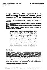
that increased energy demand for field irrigation, soil cultivation and crops production, and nonagricultural purposes, such as tools made from wood and iron. Since the industrial revolution in the nineteenth century, large amounts of energy have been required for new applications, such as steam and internal combustion engines and various electrical equipment. Figure 1.1 illustrates the change of world population and primary energy consumption from 1890 to 2010. In this period, the world population has increased by a factor of more than 4, from 1.6 to 6.8 billion people. On the other hand, the global primary energy consumption has increased by a factor of more than 17, from 31 to 539 EJ/year. Between 1890 and 2010, the per capita consumption of primary energy (expressed as power expenditure) has quadrupled from 0.61 to 2.52 kW/ capita. This amount significantly exceeds the energy of the Western food consump­ tion of about 0.2 kW/capita, which is sufficient for the human existence. However, the regional distribution of energy use is very diverse. Table 1.1 summarizes the 2010 population, total primary energy consumption, and primary energy consumption per capita (expressed as power expenditure) of several countries selected from all continents, including developed and less developed countries. The world’s highest energy consumption per capita relates to the developed countries in North America, such as Canada (12.9) and the United States (10.6), Europe, such as France (5.7), Germany (5.7), and the United Kingdom (4.8), and Asia, such as Japan (5.7 kW/cap). On the other hand, major parts of the world population consume much less energy per capita, particularly in the developing countries such as India (0.63), Bangladesh (0.21), and in Africa, such as Ethiopia (0.053 kW/cap). The highest energy consumers are China and the United States that use 19.8 and 19.3% of the world’s primary energy, respectively. To the world’s 10 highest primary energy consumers also belong Russia (5.7), India (4.3), Japan (4.3), Germany (2.7), Canada (2.5), Brazil (2.2), France (2.2), and the United Kingdom (1.7%). The top 10 countries consume more than one-third of the world’s total primary energy. Table 1.1 also presents the energy intensity of economic output that is expressed as a ratio between the primary energy use and the gross domestic product (GDP) (in US$2005). Generally, more developed countries show lower energy intensity of their economy that is mainly due to the higher efficiency of energy conversion. Some countries, such as Russia, China, and less developed countries consume more primary energy per GDP, which is largely due to a less efficient economic system. However, differences in the energy intensity are also caused by other factors, such as country size, climate, composition of primary energy supply, and differences in an industrial structure (Smil, 2000).

1.1

5

ENERGY AND THE ENVIRONMENT

TABLE 1.1 Energy Characteristics for Several Countries, 2010

Country The United States Canada Mexico Germany France The United Kingdom Russia Brazil Argentina China India Japan Bangladesh Saudi Arabia South Africa Egypt Ethiopia World

Population (million) 309.3 33.8 112.5 81.6 64.9 62.3 142.5 195.8 41.3 1,330.1 1,173.1 127.6 156.1 25.7 49.1 80.5 86.0 6,863.2

Primary Energy Consumption (EJ/year)

Primary Energy Consumption Per Capita (kW/cap)a

Energy Intensity (MJ/US$2005)

103.4 13.7 7.69 14.7 11.6 9.41

10.6 12.9 2.17 5.68 5.71 4.78

7.92 11.4 8.33 5.01 5.28 4.04

30.9 11.9 3.53 106.4 23.1 23.0 1.04 8.28 5.90 3.49 0.144 538.7

6.88 1.93 2.71 2.54 0.625 5.71 0.212 10.2 3.81 1.38 0.053 2.49

34.2 10.9 13.9 27.7 18.5 5.01 13.4 23.0 20.5 27.8 7.16 10.5

Source: EIA (2013a). a Expressed by power expenditure.

It is expected that energy consumption will significantly increase in the future. This is mostly due to two effects, namely, the expected population growth in the future and the increase of energy use per capita in less developed countries. According to the Shell energy scenarios, the global primary energy consumption in 2050 can range between 770 and 880 EJ/year, depending on the future pattern of energy consumption (Shell, 2008). The United Nations Development Program foresees in 2050 the primary energy consumption in the range of 600–1040 EJ/ year and in 2100 in the range of 880–1860, depending on the population and economic growth (UNDP, 2000). Historical energy use shows a very large change not only in the amount of consumed energy, as described above, but also in the pattern of energy sources. Human civilization has used biomass (mainly wood fuel) as a primary energy source for a long time until the beginning of the industrial revolution. The fossil fuels era began at the end of the nineteenth century when coal started to replace wood as the primary fuel. Later, other fossil fuels, such as oil and natural gas, were available in large amounts and low cost. Figure 1.2 illustrates the historical primary energy consumption pattern for the United States for the years 1850, 1930, and 2010. In 1850, wood was the dominant fuel contributing more than 90% to the primary energy consumption in the United States. Eighty years later in 1930, biomass was replaced by coal as the main fuel that contributed 58% to the primary energy consumption. The same year the remaining fossil fuels were oil (25%) and natural gas (8%), whereas the share of biomass was reduced to 6% only. Eighty years later, in 2010, fossil fuels contributed 83% to the primary energy consumption, whereas the remaining primary energy was supplied as nuclear electric (8.6%), biomass (4.4%), and other renewables (3.9%). Figure 1.2 also illustrates that over the period

Carbon Dioxide Emissions (Mton/year) 5,637 547 432 793 389 529 1,642 451 174 7,997 1,601 1,180 57.0 469 473 191 6.45 31,502

6

CHAPTER 1

BIOENERGY SYSTEMS: AN OVERVIEW

FIGURE 1.2 Historical primary energy consumption patterns (%) for the United States (source: EIA, 2011).

1850–2010, the primary energy consumption in the United States has dramatically increased from 2.5 to 103.1 EJ/year, which is due to the availability of fossil fuels. Over the same period, the primary energy consumption per person has increased from 3.4 to 10.6 kW/capita. Figure 1.3 illustrates the share of various energy sources in the global primary energy consumption for the years 1973 and 2011. For both years, the global energy pattern was dominated by fossil fuels that contributed 86.6 and 81.8%, respectively, to the global primary energy consumption. In 1973, oil (46%) was the main fossil fuel, whereas in 2011 its share was reduced to 32%. Over the period 1973–2011, the share of coal increased from 25 to 29% and that of natural gas from 16 to 21%. On the other hand, the contribution of bioenergy remained almost constant, 10.6% in 1973 and 10.0% in 2011. Other energy sources in 2011 were nuclear electric (5.1%) and various renewable energy forms (3.3%), such as hydro, geothermal, solar, and wind. It should be noticed that currently biomass is the fourth fuel in the world that has an average share of 10% in the global primary energy consumption. However, the distribution of biomass consumption is very unequally spread between developed and developing countries. The major part of biomass (about 80% of the world biomass) is consumed in Africa, Asia, and Latin America where it is used mainly for cooking and heating. The largest share of biomass in total primary energy consumption corresponds to Africa (47%), followed by Asia (25%) and Latin America (19%). In some of the least developed countries in these regions, biomass is the dominant fuel whose share is up to 80% of a country primary energy consumption (FAO, 2010). On the other hand, in the developed countries, biomass is mainly consumed for production of power, fuels, and chemicals, which is the main subject of this book.

FIGURE 1.3 Share of energy sources in the global primary energy supply (source: IEA, 2013).

1.1

ENERGY AND THE ENVIRONMENT

1.1.2 Conversion and Utilization of Energy Primary energy is not suitable for a direct use by consumers and is usually converted using an energy system into various secondary energy forms that can be either stored or transported to end users. An energy system is arranged as a chain that comprises a number of stages, as illustrated in Figure 1.4. The energy chain begins with a supply of the primary energy and ends with the final energy users. Primary energy can be supplied from the environment in various forms, such as fossil fuels (coal, oil, and natural gas), nuclear fuels (uranium), and renewable energy, such as biomass, hydropower, wind, solar, and geothermal. Currently, the primary energy is mainly supplied from fossil fuels (81.6% in 2011) (see Fig. 1.3), as mentioned in Section 1.1.1. Conversion of the primary to the secondary energy (also called energy carriers) takes place in various plants and devices, such as power and combustion plants, petro- and biorefineries, and fuel plants. The most common energy carriers are electricity, heat, cold, and various fuels, such as hydrocarbons [gasoline, diesel, or liquefied petroleum gas (LPG)], alcohols, and hydrogen. The share of electricity as an energy carrier has substantially increased over the years, which is due to its easy transmission and use flexibility. Currently, about 40% of fossil fuels is converted into electricity compared to less than 2% in 1900 (Smil, 2000). In 2011, the amount of produced electricity was equal to 79.7 EJ, which was mainly generated in fossil fuel power plants (68.0%), followed by hydroelectric plants (15.8%), nuclear power plants (11.7), and renewable sources (4.5%) (IEA, 2013). Hydrocarbon fuels are other important energy carriers that are produced in oil refineries. In 2011, the amount of 3896 Mton of hydrocarbon fuels were produced, namely, middle distillates (34.7%), motor gasoline (23.1%), fuel oil (13.2%), LPG/ ethane/naphtha (9.5%), aviation fuels (6.4%), and other products (13.1%) (IEA, 2013). The advantage of hydrocarbon fuels is that they can be easily transported and stored, whereas electricity can be easily transmitted but is very difficult to store. In the last stage of the energy chain, energy carriers are consumed by the end users that can be classified into several sectors, as shown in Figure 1.5. This figure illustrates the proportions of the primary energy use in 2010 in four major energy end-use sectors. Notice that Figure 1.5 refers to the primary energy and comprises not only the direct use of energy carriers but also the primary energy consumption required for the production of energy carriers and their transmission and distribu­ tion, including appropriate energy losses, for example, electricity losses. The highest share of the primary energy consumption (51.0%) corresponds to the industrial sector, mainly for the production of bulk materials, such as chemicals,

FIGURE 1.4 Schematic of major stages of an energy chain.

7

8

CHAPTER 1

BIOENERGY SYSTEMS: AN OVERVIEW

FIGURE 1.5 Proportions (%) of primary energy use in 2010 in various world economy sectors (source: EIA, 2013b).

iron and steel, aluminum, pulp and paper, and cement. Transportation sector consumes 19.7% of the primary energy, which almost exclusively (95%) is supplied from oil-based fuels (GEA, 2012). Road transport is responsible for almost 70% of the primary energy consumption in the transportation sector. The remaining amounts of the global primary energy are consumed by the residential (17.4%) and commercial sectors (11.9%). The largest amounts of primary energy in the residential sector are used for space heating (28%) and cooling (15%), water heating (13%), lighting (10%), and electronic devices (8%) (GEA, 2012). In the commercial sector, the largest primary energy share corresponds to lighting (20%), space heating (16%) and cooling (14%), ventilation (9%), and refrigeration (7%).

1.1.3 Fossil Fuel Resources Fossil fuels (coal, petroleum, and natural gas) are at present the major source of energy as they supply more than 80% of the global primary energy. Two serious global problems relate to fossil fuels, namely, the fast depletion due to the increased use and the environmental damage due to atmospheric pollution and global warming. Among fossil fuels, oil (petroleum) has the largest share (32%) in global primary energy supply exceeding that of coal (29%) and natural gas (21%), as indicated in Figure 1.3. Petroleum is a liquid mixture of hydrocarbons and other organic compounds with various molecular weights. Crude oil is found in geological reservoirs under the ground or seabed, mainly in Middle East, North America, Russia, North and West Africa, and South and Central America. Crude oil is refined in refineries into various hydrocarbon fractions that are used either for manufacturing of motor fuels (kerosene, gasoline, diesel, motor oils) or chemicals, mainly plastics. Liquid hydro­ carbons can also be recovered from the unconventional resources, such as oil shales and tar sands. Coal was historically the first fossil fuel that began to replace wood at the end of the nineteenth century. The main combustible substance in coal is carbon whose content varies from about 60% (lignite or brown coal) to more than 90% (anthracite). The remaining constituents are mineral ashes, moisture, and sulfur. Similar to crude oil, coal is found in various parts of the world, mainly in the United States, Russia, China, Australia, Germany, Poland, and South Africa. The principal application of coal is for generation of electricity and heat. Some amounts of coal are liquefied into hydrocarbon fuels or gasified into synthesis gas (syngas) that is used to produce chemicals, such as Fischer-Tropsch (F-T) fuels and methanol. Natural gas primarily contains methane and small amounts of higher alkanes as combustible substances in addition to carbon dioxide, nitrogen, and hydrogen sulfide. Natural gas is found in reservoirs under the ground and in seabed, very often in proximity to crude oil. Unconventional natural gas reservoirs also exist as

1.1

ENERGY AND THE ENVIRONMENT

9

FIGURE 1.6 Global proven fossil fuel reserves and reserves-to-production ratio (R/P) in 2012 (source: BP, 2013).

gas trapped in shale rocks and sandstones as well as at the bottoms of oceans as methane hydrates. In the last years, natural gas became the preferred fossil fuel, mainly due to easy and clean combustion and very high calorific value. The main application of natural gas is generation of electricity in power plants and heat for domestic and residential purposes. Large amounts of natural gas are also used as a chemical feedstock for manufacturing of hydrogen, which is applied to produce ammonia, artificial fertilizers, and methanol. The amounts of fossil fuels are finite and they become depleted due to increased energy consumption, as described in Section 1.1.1. Figure 1.6 illustrates the existing proven reserves of coal, oil, and natural gas as well as reserves-to­ production ratio for these fuels estimated for 2012. According to these estimates, the proven reserves-to-production ratio (R/P) is 109 years for coal, 53 years for oil, and 56 years for natural gas. It should be noticed that the reported R/P ratios are estimated using the reserves and production data known in 2012. However, the prediction of fossil fuels depletion should be treated with some caution due to two future uncertain effects. First, the global energy consumption is expected to increase in the future that can reduce the estimated depletion time. Second, the possibility of new discoveries and exploration of ultimate resources can extend the depletion time. The historical fossil fuels reserves data indicate that over the past 20 years, the R/P ratio for coal has decreased from 229 to the current 109 years, whereas the respective values for oil has increased from 43 to the current value of 53 years and for natural gas the R/P ratio has remained almost constant (58 years in 1992 and 56 years in 2012) (BP, 2013). Finally, it should be noticed that the global nuclear energy resources are more abundant than those for the fossil fuels; however, they are also limited (Fay and Golomb, 2002). The nuclear resource life is estimated about 50 years for high-grade uranium ores and several centuries for low-grade ores. On the other hand, a much longer resource life of several millennia is estimated for the global resources of thorium that can be used in breeder reactors.

1.1.4 Environmental Impact of Fossil Fuels Use The massive use of fossil fuels has deleterious effects on the environment and human health. These effects are associated with all stages of a fossil energy chain, starting from the fossil fuels exploration, through transportation and storage, to the final use, namely, combustion. Moreover, the environmental degradation caused by fossil fuels takes place at various scales where fossil fuels are used, such as households, communities, regional, and global. The first deleterious effects of fossil fuels on the environment already occur during fuel exploration. Mining of coal is associated with numerous fatal accidents

10

CHAPTER 1

BIOENERGY SYSTEMS: AN OVERVIEW

as well as landscape pollution by spoil heaps and water pollution by contaminants, such as heavy metals and acidic compounds. Transport of oil by tankers results in dangerous accidents that lead to serious water pollution problems. The most serious environmental effects of fossil fuels are due to their combus­ tion, namely, air and water pollution and global warming. Air pollution resulting from coal combustion was already observed from the beginning of fossil fuels use in the late nineteenth century as smog in large towns. During fossil fuels combustion, a number of pollutants are formed, such as sulfur dioxide, nitrogen oxides, carbon monoxide, and fine particles, which damage human health. Moreover, the abovementioned primary pollutants can be converted by sunlight to photo-oxidants (ozone, ketones, and aldehydes), which have a negative impact on human health and some materials. Acidic air pollutants, such as sulfur and nitric oxides, can react with water present in the atmosphere to form sulfuric and nitric acids, which are deposited as acid rain on land, lakes, and rivers. Acid rain has harmful effects on soil quality as well as on aquatic life. The use of fossil fuels also results in water and land pollution. Water quality can be deteriorated by acids and heavy metals drainage from coal mines, acid rains containing sulfur and nitrogen oxides from the fuel combustion in power plants, and by heating up surface waters, such as lakes and rivers as a result of heat removal from the power plants. Land pollution is mainly due to deposits from coal mining, particularly from the surface mining. The most serious environmental problem due to the fossil fuel use occurs at the global scale as climate change, namely, the global warming. This problem was already known since the early 1960s, later often called in question, but in recent years widely recognized as caused by human activity. The global warming results in an increase of the average Earth’s surface temperature due to the greenhouse effect. The greenhouse effect is caused by trapping of the outgoing solar radiation from the Earth’s surface by “greenhouse gases” such as water, carbon dioxide, methane, and nitrogen oxides, which accumulate in the atmosphere. The increase of the concentration of greenhouse gases in the atmosphere, mainly carbon dioxide, is a consequence of combustion of fossil fuels. Global carbon dioxide emissions from the consumption of energy increased from 2 billion ton CO2 in 1900 to 19 billion ton CO2 in 1980, and reached more than 31 billion ton CO2 in 2010. Table 1.1 lists the CO2 emissions from the consumption of energy for various countries. The largest CO2 emissions correspond to countries that are the largest energy users as well as countries with the largest share of fossil fuels as primary energy source. In 2010, the largest CO2 amounts were emitted by China (7,997 Mton), the United States (5,637 Mton), Russia (1,642 Mton), India (1,601 Mton), Japan (1,180 Mton), and Germany (793 Mton). Figure 1.7 illustrates the increase of the atmospheric CO2 concentration from 1000 till 2013. The historical data indicate that the atmospheric CO2 concentration

FIGURE 1.7 Atmospheric carbon dioxide concentrations, 1000–2013 (source: CDIAC, 2013).

1.1

ENERGY AND THE ENVIRONMENT

11

was quite stable (about 280 ppm) until the beginning of the industrial revolution when the intensive use of fossil fuels began. Since 1900, the atmospheric CO2 concentration increased gradually until the current level of almost 400 ppm. Based on the projections of the future increase of CO2 concentration, it is expected that the average Earth’s surface temperature can increase in the twenty-first century about 1–3°C (IPCC, 2013). The expected global changes due to this temperature increase are the sea level rise and climatic changes, such as altering precipitation patterns and increased frequency of hurricanes. Global warming can be controlled by reduction of atmospheric CO2 emissions from fossil fuels and replacing fossil with carbon-free renewable energy. Carbon dioxide emissions from fossil fuels can be reduced by energy efficiency improve­ ment as well as CO2 capture and sequestration. In the last years, various CO2 reduction methods are under development, such as oxy-combustion, solvent separation, and membrane separation. After the capture, CO2 can be sequestrated in depleted oil and gas reservoirs or in deep oceans and deep aquifers (Fay and Golomb, 2002).

1.1.5 Renewable Energy In recent years the interest in renewable energy is growing due to serious problems related to fossil fuels use, such as fast depletion and environmental damage. Many sources of renewable energy, such as biomass, hydropower, and wind have been used by humans for a long time before the fossil era began. At present the traditional renewable energy sources are further technologically advanced and new renewable sources, such as direct solar, geothermal, ocean, and tidal are being developed (Lund, 2014; Twidell and Weir, 2015). Compared to fossil fuels, renewable energy has many advantages. Most renew­ able energy forms originate directly or indirectly from the solar radiation, are more uniformly distributed geographically, have a lower environmental impact, and are less subjected to price fluctuations. In 2011, all renewable energy sources were responsible for 13.3% of the global primary energy supply that corresponds to 73 EJ. Figure 1.8 illustrates the shares of various energy sources in the global renewable primary energy supply. Biomass clearly dominates the current renewable energy pattern at a share of 79%. Biomass energy originates from photosynthesis that produces the organic matter present in a variety of plants, crops, algae, and trees. Although biomass energy is mainly limited to the traditional use as a cooking and heating fuel in developing countries, in the last decades biomass is increasingly applied to produce modern energy carriers as electricity, biofuels, and chemicals. The second most significant renewable energy is hydropower at a share of about 18%. Hydropower utilizes the potential energy of water flowing in rivers and streams. Traditionally, hydropower was used to produce mechanical energy for irrigation, and later to drive various machines, mainly industrial mills. Presently,

FIGURE 1.8 Shares (%) of energy sources in the global renewable primary energy supply in 2008 (source: IPCC, 2012).

12

CHAPTER 1

BIOENERGY SYSTEMS: AN OVERVIEW

hydropower is utilized to generate electricity at a variety of scales, ranging from small of few kilowatt to large of several gigawatt. Wind is another traditional renewable energy that in the past was mainly utilized to produce mechanical power for grain milling and propelling ships. At present the kinetic energy of wind is converted in wind turbines to generate electricity and to produce mechanical power for water pumping. The generating capacity of wind turbines has increased from about 30 kW in the 1970s up to several megawatt in recent years. Modern wind farms that consist of many wind turbines are located either onshore or offshore in various parts of the world. Direct solar energy can be utilized in a variety of ways to generate heat and electricity. The most common way to generate heat is by using solar thermal collectors whose surface is heated by irradiation. The produced heat can be either directly utilized for heat purposes, usually a hot water production, or to generate a high-temperature air or steam that can be used to generate electric power. Elec­ tricity can also be directly generated from solar energy using photovoltaic cells. Photovoltaics are currently used in small systems in houses (size 0.05–5 kW) or larger systems in solar power plants (10 kW–500 MW). Geothermal energy can be recovered in many locations from the Earth’s crust. The extracted heat is applied either directly for heating purposes or indirectly to generate electricity. Heat can be recovered at various temperature levels ranging from low (30–100°C) up to high temperatures (above 180°C). The most geothermal power plants operate in the United States, Philippines, Italy, Mexico, Indonesia, and Japan. Various forms of renewable energy are based on effects occurring in the oceans. They include tidal energy, wave energy, and ocean thermal gradient. The tidal energy utilizes the regular tidal rise and fall of the ocean level due to gravitational forces between Earth, Moon, and Sun. Wave energy originates from winds blowing over the ocean whose kinetic energy is converted into wave movement. Ocean thermal gradient is a temperature difference between the temperature of the warmer ocean surface that is directly heated by the sun and much lower temperature in the deep ocean, below 1000 m. The temperature difference of 20–25°C can be utilized to generate electric power. At present several prototypes of tidal and wave energy plants are in operation, whereas there are no plants based on the ocean thermal gradient. Table 1.2 lists the current use (2010) and the global technical potential of renewable sources estimated for 2050. It should be noticed that the reported estimates of the future potential are subjected to a wide range of uncertainties.

TABLE 1.2 Global Potential (2050) of Renewable Energy Sources

Renewable Energy Biomass Hydropower Wind Direct solar Geothermal Ocean Source: IPCC (2012). a

Electricity. Heat.

b

Current Use 2010 (EJ/year)

Potential 2050 (EJ/year)

Current Use 2010/Potential 2050 (%)

Potential 2050/Global Primary Energy Consumption 2010 (%)

55 12.4 1.1 0.54 0.54

50–500 50–52a 85–580a 1,575–49,837 118–1,109a 10–312b 7–331

11–110 24–25 0.2–1.3 0.03–0.001 0.05–0.5 0.2–5 0.03–0.2

9–93 9–10 16–108 292–9,251 22–206 2–58 1–61

0.011

1.2

13

BIOMASS AS A RENEWABLE ENERGY SOURCE

However, it can be concluded that a significant potential exists for all renewable energy sources that substantially exceed the current use. At present biomass and hydropower are the most used energy sources in comparison with their respective future potential. On the other hand, the direct solar and ocean energy show the lowest ratio between the current and potential uses. Finally, it can be concluded that renewable energy sources can significantly cover the future global energy demand. Particularly, the direct solar energy is able to supply several hundreds to thousands percent more energy compared to the present global primary energy consumption (538.7 EJ/year, see Table 1.1). The future energy potential of other renewable sources, particularly biomass, wind, and geothermal, is comparable with the present global primary energy consumption.

1.2 BIOMASS AS A RENEWABLE ENERGY SOURCE 1.2.1 Introduction Biomass is an organic material that is produced in plants (crops, trees, and algae) by photosynthesis. During photosynthesis, atmospheric carbon dioxide and water are converted by sunlight into organic compounds, according to the following general reaction: CO2 ‡ H2 O ‡ light ! …CH2 O† ‡ O2

(1.1)

The primary organic products of photosynthesis are simple carbohydrates (sugars) that are composed from the building blocks (CH2O) and can subsequently be converted into a variety of organic products, such as polysaccharides (starch, cellulose, and hemicellulose), lignin, lipids, proteins, and other compounds. Biomass always has been and is still used by the humanity for food and feed purposes as well as for energy and materials, as shown in Figure 1.9. At present biomass accounts for about 10% of the global primary energy consumption. The majority of biomass is used in the traditional way in the developing countries for cooking and heating. In recent years, there is an increased interest in modern use of biomass as a renewable energy source, which includes power and heat generation as well as production of transport fuels and chemicals. Biomass as an energy source has numerous advantages. First, it is renewable and CO2 neutral. Carbon dioxide that is formed during the final use of biomass is

FIGURE 1.9 Biomass energy chain from growth to end-products.

14

CHAPTER 1

BIOENERGY SYSTEMS: AN OVERVIEW

released to the atmosphere and subsequently fixed back to the plants by photo­ synthesis, as shown in Figure 1.9. Second, biomass is the only renewable carbon source that can replace not only fossil fuels in the production of energy carriers but also many important chemicals. Third, biomass enables energy storage, similarly as fossil fuels, whereas this is not directly possible for many other renewable energy sources, such as wind or solar. Finally, a wide range of biomass resources are available in most parts of the world. On the other hand, the use of biomass is accompanied by possible drawbacks, mainly limitations of land and water, and competition with food production. Therefore, it is attractive to use waste biomass from food, feed, and materials production (see Fig. 1.9) as feedstock for energy production. The production of biomass involves high logistics costs due to the low-energy density of biomass. Moreover, biomass suffers from a very low conversion effi­ ciency of sunlight into chemical energy through photosynthesis. For biomass-based systems, a key challenge is thus to develop efficient conversion technologies that can compete economically with fossil fuels.

1.2.2 Historical Development and Potential of Bioenergy Biomass has always played an important role in the history of humankind. It has been used and will remain the principal source of our food and many materials. Furthermore, biomass was the primary fuel used by humankind for the thousands of years from the beginning of civilization until the nineteenth century when the fossil era began. The major use of biomass was as a fuel for cooking and heating. It is interesting to notice that at the beginning of the nineteenth century, the first automobiles were fueled by biomass-derived fuels, such as ethanol and peanut oil. Since the end of the nineteenth century, biomass was replaced by fossil fuels, first by coal and later in the twentieth century by oil and natural gas. The oil crisis in the 1970s has initiated the renewed interest in biomass and other renewable energy sources such as wind and solar. At present biomass provides 55 EJ/year of the primary energy that corresponds to about 10% of the global primary energy consumption. Figure 1.10 shows the distribution of the primary biomass energy use that can be classified as the traditional as well as modern applications. The traditional biomass use as firewood for heating and cooking (76%) still dominates the current bioenergy pattern. Biomass is the main energy source in many developing countries where it is responsible for the major part of the residential energy use in Africa (85%), Asia (75%), and Latin America (45%) (Sagar and Kartha, 2007). As shown in Figure 1.10, the modern biomass use accounts only for about 25% of the global primary biomass energy consumption. These include mainly a largescale commercial generation of heat and electricity as well as production of

FIGURE 1.10 Primary biomass energy use in 2009 (source: GEA, 2012).

1.2

BIOMASS AS A RENEWABLE ENERGY SOURCE

15

transport fuels such as bioethanol and biodiesel. In the developed countries, modern biomass applications account for 3–4% of the total energy consumption, although in some countries, such as Sweden, Finland, and Austria, biomass contribution reaches 15–20% (GEA, 2012). In future biomass can contribute much more to the global primary energy consumption as the amount of new biomass formed by photosynthesis is significantly larger than the current yearly biomass consumption. Solar radiation is the main source of energy used in the photosynthetic production of biomass. The total amount of energy of the extraterrestrial solar radiation that reaches the Earth is enormous—174,000 TW (about 5.5 mln EJ/year). About half of the extraterrestrial solar radiation is lost in the atmosphere due to reflection and absorption effects. The remaining part of the solar radiation energy equal to 86,000 TW (about 2.7 mln EJ/year) is incident on the Earth’s surface and is used for surface heating and water evaporation as well as it is available for photo­ synthesis. However, only a very small part of the incident solar radiation is transformed by photosynthesis into chemical energy in new biomass that amounts about 2870 EJ/year (90.9 TW), which is defined as the net primary productivity (NPP) (see Section 3.4.1). The terrestrial part of the NPP amounts about 1960 EJ/year that corresponds to 68% of the global NPP. Currently, humans appropriate about 373 EJ/year of biomass, which is about 19% of the terrestrial NPP. Figure 1.11 illustrates the human appropriation of the global terrestrial biomass. Less than 60% of biomass is harvested, namely, as plant-based food (28 EJ/year), feed (129 EJ/year), wood (36 EJ/year), and other uses (26 EJ/year). More than 40% of the remaining part of the biomass (154 EJ/year) is destroyed by human-induced fires or left unused as underground biomass, cropland residues, felling losses in forests, and harvest losses. The final biomass use as food for humans, timber, and paper and bioenergy accounts for about 40% of the harvested biomass. Most energy scenarios refer to 2050 and significantly differ in estimates of the future global bioenergy availability, ranging from low values of about 40 EJ/year up to high values of about 1100 EJ/year. These discrepancies result from different assumptions made regarding future land availability, population growth, food consumption, biomass yield, and bioenergy conversion efficiency. The lowest biomass potential estimate (about 40 EJ/year) corresponds to the pessimistic scenario in which no more land is available for energy farming, whereas the highest estimate (about 1100 EJ/year) corresponds to the optimistic scenario of the intensive agriculture concentrated on better quality soils. The most realistic estimate that is based on the review of several studies assumes the bioenergy potential in 2050 ranging from 250 to 500 EJ/year (Heinimö and Junginger, 2009). According to this estimate, the future biomass feedstocks will be available mainly

FIGURE 1.11 Human appropriation of the global terrestrial biomass in 2000 (source: GEA, 2012).

16

CHAPTER 1

BIOENERGY SYSTEMS: AN OVERVIEW

as energy crops cultivated on current agricultural land, biomass produced on marginal lands, forest and agricultural residues, dung, and organic wastes. The projected potential for biomass will be mainly available in the climate regions that favor biomass growth, such as Latin America, Sub-Saharan Africa, Eastern Europe, and North and North-East Asia, whereas most of the biomass will be converted in industrial OECD countries, such as the United States, Europe, and Japan. This will stimulate the international trade in bioenergy and development of biomass markets.

1.2.3 Biomass Resources Biomass feedstocks are very diverse as they originate from various sources and therefore can be classified in different ways. From the viewpoint of the biomass origin, feedstocks can be classified as virgin (naturally growing terrestrial and aquatic crops) and waste biomass (by-products from biomass processing). Biomass also differs in the content of its constituting components, such as carbohydrates, lignin, lipids, and proteins, which results in a classification into sugar, starch, oil, and lignocellulosic crops. In this section, we classify biomass feedstocks based on their economic competition as an energy source compared to the traditional biomass use for food and materials. Table 1.3 shows the classification of biomass feedstocks that are grouped into first-, second-, and third-generation feedstocks as well as waste biomass. The firstgeneration biomass includes food and fodder crops that are essential for the food chain, such as sugar, starch, and oil crops. At present some of these crops are used for production of biofuels, such as ethanol and biodiesel. The competition between various uses of the first-generation biomass has led in the past to a food versus fuel debate that has negatively influenced the social picture of biofuels. Therefore, more promising are next-generation feedstocks, particularly the second-generation lignocellulosic and the third-generation aquatic biomass. The

TABLE 1.3 Classification of Biomass Feedstocks Feedstock Generation First

Type

Crops

Food and fodder crops

Sugar crops Starch crops Oil crops Fodder

Second

Lignocellulosic crops

Woody

Examples Sugarcane, sugar beet, sweet sorghum Corn, wheat, potato, rye, cassava, triticale Soybean, rapeseed, oil palm, cottonseed, peanut, sunflower Lucerne, grass

Herbaceous

Short-rotation crops: willow, poplar, eucalyptus, acacia Miscanthus, switchgrass, reed canary grass

Third

Aquatic

Microalgae Macroalgae Water plants

Chlorella, Spirullina Seaweed, kelp Water hyacinth, salt marshes, sea grass

Wastes

Natural

Agricultural Forest Municipal

Animal manures, field residues, processing residues Logging residues, excess small pole trees Municipal solid waste (MSW), sewage sludge, demolition wood, food waste, waste oil Pulp and paper industry (black liquor), sludges

Man-made

Industrial

1.2

BIOMASS AS A RENEWABLE ENERGY SOURCE

second-generation lignocellulosic biomass are energy crops that can be cultivated on a large scale. They include short-rotation woody crops, particularly willow, poplar, and eucalyptus, as well as herbaceous crops, particularly fast-growing grasses, such as switchgrass, miscanthus, and reed canary grass. The lignocellulosic biomass does not compete with food crops; however, it requires land that is a scarce resource and large energy plantation can have a negative environmental impact due to the land use change. Aquatic biomass is an attractive energy source as it does not compete with food and land use. It includes various categories, such as microalgae, macroalgae, and water plants. Cultivation of microalgae is particularly promising due to very high yields exceeding that of most terrestrial crops. Biomass wastes are the last group of feedstocks that can be divided into natural and man-made wastes. Large volumes of agricultural wastes are generated during harvesting and processing of crops, such as straw and corn stover as well as from livestock farming such as animal manures. Forest residues are a significant source of lignocellulosic biomass that is collected as logging residues or forest slash. Manmade waste biomass, such as residential wastes (municipal solid waste (MSW) and sewage sludge) as well as various industrial wastes, particularly from the paper and pulp industry (black liquor), are abundant and nonexpensive biomass feedstocks.

1.2.4 Biomass Properties The most important biomass properties that determine the suitability of feedstocks for conversion process are proximate and ultimate analysis, energy content, and chemical composition. Table 1.4 lists the above-mentioned parameters for typical biomass feedstocks, including woody and herbaceous biomass, aquatic biomass, and biomass residues and wastes. Proximate analysis specifies a content of moisture, organic matter, and ash in biomass feedstocks. The moisture content in fresh biomass (as received) is usually quite high, typically about 50% for green wood, 50–80% for green crops, such as maize, sugarcane, and rapeseed, and very high (more than 80%) for aquatic biomass and liquid wastes. Moisture content in wet biomass is usually reduced to few percent either by natural or thermal drying. On the other hand, a slightly wet biomass is a suitable feedstock for steam gasification or even a wet biomass for the supercritical water (SCW) gasification (see Section 6.7). Ash content is typically about 1% for woody biomass, several percents for herbaceous and aquatic biomass, and much higher for biomass wastes and resi­ dues. During biomass conversion, the high ash content can cause serious operating problems, such as ash melting and sintering during combustion of herbaceous biomass (grasses and straw). Ash contains many metal oxides, particularly calcium, potassium, phosphorus, magnesium, and silicium. Organic fraction of biomass is a source of crucial elements, such as carbon and hydrogen, and energy for all chemical and biochemical conversion processes. It is quite interesting to note that carbon, hydrogen, and oxygen content of most terrestrial biomass feedstocks fall in a relatively narrow range, despite a wide variety of plants, wood, and crop species. Carbon content for the virgin terrestrial biomass varies in the interval of 48–52 wt%, oxygen: 40–44 wt%, and hydrogen 5–7 wt%. On the other hand, aquatic and waste biomass feedstocks contain more nitrogen and sulfur and less oxygen compared to the virgin biomass. Energy content of biomass feedstocks is usually expressed either as the lower heating value (LHV) or the higher heating value (HHV). The difference between both heating values is due to various assumptions regarding the reference state of water in biomass combustion products that is either vapor (LHV) or liquid (HHV).

17

18

CHAPTER 1

BIOENERGY SYSTEMS: AN OVERVIEW

TABLE 1.4 Typical Proximate and Ultimate Analysis and HHV of Biomass Feedstocks Proximate Analysis (wt% ar) Feedstock

Ultimate Analysis (wt% daf) C

H

O

N

S

HHV (MJ/kg dry)

0.5 5.5 2.0 0.5 1.4

50.6 52.8 51.6 52.3 49.8

6.1 6.1 6.1 6.1 6.1

42.9 40.5 41.7 41.2 43.4

0.3 0.5 0.6 0.3 0.6

0.1 0.1 0 0.1 0.1

20.1 19.5 20.0 20.5 29.8

85.9 84.1 83.6

2.7 8.2 4.5

49.2 49.4 49.7

6.0 6.3 6.1

44.2 42.7 43.4

0.4 1.5 0.7

0.2 0.2 0.1

20.1 18.9 19.8

12.4 10.6 10.4 43.6 6.4

81.1 73.3 87.7 39.2 50.3

9.5 16.1 1.9 17.2 43.3

48.8 49.3 49.8 50.2 50.9

5.6 6.1 6.0 6.5 7.3

44.5 43.7 43.9 34.6 33.4

1.0 0.8 0.2 5.2 6.1

0.1 0.1 0.1 0.9 2.3

17.1 16.0 19.4 14.2 10.7

90.0 90.0

7.8 6.1

2.2 3.9

53.0 45.3

6.8 6.1

37.2 46.1

2.5 2.0

0.5 0.6

16.0 10.0

7.3 0

84.6 100

8.1 0

75.6 44.4

5.9 6.2

15.7 49.3

1.8 0

1.1 0

28.3 17.5

Moisture

Organic Matter

Ash

Wood Oak wood Pine chips Poplar Spruce wood Willow

6.5 7.6 6.8 6.7 10.1

93.0 86.9 91.2 92.8 88.5

Grass Miscanthus Reed canary grass Switchgrass

11.4 7.7 11.9

Residues and wastes Straw Rice husks Sugarcane bagasse Manure Sewage sludge Aquatic Water hyacinth Giant brown kelp Other Bituminous coal Pure cellulose

Sources: Klass (1998); Ptasinski et al. (2007); Song et al. (2011); Vassilev et al. (2010).

For most biomass feedstocks, typical HHV values range from 10 to 20 MJ/kg of dry feedstock, whereas the lower values correspond to aquatic and waste biomass and the higher values to virgin terrestrial feedstocks. The energy content of biomass feedstocks can be estimated from several correlations based on the ultimate analysis of biomass. The HHV of biomass (in MJ/kg dry) can be estimated with a reasonably good accuracy (+/ 3%, but worse for wastes) from a simple correlation (Klass, 1998): HHV ˆ 45:71 zC

2:7

…MJ=kg dry†

(1.2)

where zC is the mass fraction of carbon in biomass on dry basis. A more accurate correlation (absolute error 1.5%) for biomass fuels having a wide range of elemental composition is proposed by Channiwala and Parikh (2002): HHV ˆ 34:91 zC ‡ 117:83 zH ‡ 10:05 zS

10:34 zO

1:51 zN

2:11 zA

…MJ=kg dry† (1.3)

where zi denote the mass fractions of C, H, S, O, N, and ash in biomass on dry basis. Chemical composition of biomass is important for biochemical conversion processes, such as production of biofuels (ethanol and biodiesel) and biorefinery

1.2

19

BIOMASS AS A RENEWABLE ENERGY SOURCE

TABLE 1.5 Chemical Components of Selected Biomass Feedstocks (wt%) Component Simple carbohydrates Complex carbohydrates C6 Complex carbohydrates C5 Lignin Proteins Lipids Ash

Sugarcane

Maize

Rapeseed

Oil Palm

Grass

Willow Tree

33.4 27.6 22.6 4.8 2.9 1.3 7.4

32.3 23.9 14.8 9.7 10.6 1.7 7.1

1.7 25.4 16.8 5.7 26.3 16.0 8.1

0 28.0 10.4 11.1 3.1 38.1 9.4

10.9 29.8 21.3 2.9 19.2 4.3 11.6

0 49.5 22.8 22.9 2.0 0 2.9

Source: Brehmer (2008).

processes. Table 1.5 summarizes main chemical components of typical biomass feedstocks. Most biomass is composed of carbohydrates (saccharides) that exist in biomass as various chemical compounds, such as simple carbohydrates (sucrose, fructose, and starch) and complex carbohydrates (cellulose, hemicellulose, and pectin). The classification of carbohydrates into simple and complex corresponds to their processing ability by fermentation to ethanol (Brehmer, 2008). Carbohydrates can be further divided into C6 and C5 carbohydrates depending on the number of carbon atoms in simple sugar molecules, which are the buildings blocks of complex carbohydrates. Most terrestrial biomass feedstocks shown in Table 1.5 are composed of cellulose (C6 carbohydrates) and hemicellulose (mixture of C6 and C5 carbohydrates). Woody biomass has the highest cellulose and hemicellulose content and is also rich in lignin (aromatic polymers). On the other hand, sugar and starchy crops, such as sugarcane, sugar beet, and corn, are abundant in simple carbohydrates and therefore are used as feedstocks for bioethanol production. Chemistry of processing of simple and complex carbohydrates into ethanol is described in more detail in Section 8.1.4. Other important chemical biomass compounds are proteins and lipids. Proteins are large complex compounds built from amino acids whose carboxyl (-COOH) and amino ( NH2) groups are held together by peptide bonds. Protein-rich biomass feedstocks are rapeseed, sunflower, lucerne, and grasses. Proteins derived from biomass can play an essential role in the production of nitrogen compounds in future biorefineries (see Chapter 17). Lipids are various chemical compounds, mainly triglycerides of fatty acids, which are used for production of biodiesel fuels (see Chapter 7). The most important triglycerides are present in vegetable oils of crops such as rapeseed, soybean, sunflower, and oil palm. The chemistry of triglycerides is discussed in more detail in Section 7.1.3.

1.2.5 Environmental Impact of Bioenergy Biomass as a renewable energy source has several positive environmental impacts. The most important environmental effects result from the replacement of fossil fuels and the associated benefits, such as reduction of greenhouse gases (GHG) emis­ sions, environmental pollution, and saving depletable fossil energy. However, the use of biomass, similarly as other renewable energy, also has some negative impact on the environment, which should be quantified using preferably the life cycle assessment (LCA) if the renewable energy would replace fossil fuels in the future. Biomass should be completely carbon neutral as carbon dioxide generated from the final use of bioenergy, which is principally combustion, is fixed back to crops by

20

CHAPTER 1

BIOENERGY SYSTEMS: AN OVERVIEW

FIGURE 1.12 Carbon flows for bioenergy systems.

photosynthesis. However, at present fossil fuels and related fossil carbon flows are also used in all stages of bioenergy chain, as illustrated in Figure 1.12. During biomass cultivation and harvesting, fossil energy is used for the production of fertilizers and pesticides, as well as a fuel for water management systems (irrigation and drainage) and harvesting machinery. Subsequently, biomass feedstocks are usually transported to processing facilities where they are converted into electricity, heat, biofuels, or biochemicals. Transport of biomass feedstocks requires fossil fuels for trucks, trains, and ships. During biomass conversion, an additional fossil energy is used as heat or electricity. All the above-mentioned fossil carbon flows result in the atmospheric carbon dioxide emissions from bioenergy chains in addition to the main CO2 flows due to combustion and photosynthesis, indicated in Figure 1.12 with the gray arrows. The majority of fossil CO2 emissions from bioenergy chains originate from the produc­ tion of fertilizers and pesticides, as discussed in Chapter 4. It is generally recognized that life cycle GHG emissions from bioenergy chains are remarkably lower than the corresponding emissions from fossil energy chains. The lowest GHG emissions are from the generation of bioelectricity that are about 15–30 g CO2 eq/MJ compared to the range of 100–200, 200–300, and 300–500 g CO2 eq/MJ for the electricity generated from natural gas, oil, and coal, respectively (IPCC, 2012). Similar results are obtained for heat generation from biomass where the GHG emissions are in the range of 5–20 g CO2 eq/MJ compared to 70–85, 90–120, and 100–200 g CO2 eq/MJ for heat generated from natural gas, oil, and coal, respectively. In case of biofuels, GHG emissions are also reduced compared to fossil fuels but the reductions are lower than those for electricity and heat. Life cycle GHG emissions for sugarcane ethanol and corn ethanol ranges from 15 to 70 g CO2 eq/MJ compared to that for petroleum gasoline of 85–110 g CO2 eq/MJ. Similarly, life cycle GHG emissions from biodiesel range from 25 to 125 g CO2 eq/MJ, whereas that for petroleum diesel are 75–120 g CO2 eq/MJ. The above-described GHG emissions do not account for the additional CO2 emissions due to land use changes when biomass growing on the existing land is replaced by the new one. The global amounts of carbon fixed in the soil are twice that of the carbon present in the atmospheric CO2 and the land use change can result in a significant altering of the carbon balance. The additional carbon emissions occur when land with natural biomass is converted into intensive agriculture with annual crops. On the other hand, conversion of land with annual crops into land with perennial crops results in more carbon deposit into the soil. Generally, waste biomass feedstocks perform environmentally better than the virgin biomass that is due to two effects. First, use of wastes as biomass feedstocks

1.2

BIOMASS AS A RENEWABLE ENERGY SOURCE

solves the waste disposal problems. Second, energy content of waste biomass is quite high that results in a generation of the additional energy. Moreover, waste biomass feedstocks do not require new land and do not compete with food production.

1.2.6 Economics of Bioenergy An exact comparison between costs of bioenergy and fossil energy is quite difficult. First, biomass feedstocks and conversion technologies are very diverse and have different costs and benefits. Second, fossil fuel prices are subjected in last decades to frequent and great fluctuations due to various factors, such as economic development and regional or political situation. Finally, the current fossil prices do not represent the true cost as some negative externalities associated with fossil energy due to environmental and health impact, military actions, cannot be exactly quantified. Generally, currently made bioenergy products are more expensive than the fossil ones. However, some biofuels, such as sugarcane ethanol, as well as electricity and heat generated from waste biomass are already competitive with fossil energy. On the other hand, bioenergy is expected to offer several economic and social advantages when it will replace on a full scale fossil fuels in future. The develop­ ment of new biomass production and conversion facilities will stimulate employ­ ment in agriculture, forestry, and chemical processing. Biomass production and conversion are more geographically distributed than fossil fuels and, therefore, more countries will profit from this new economic development. Feedstock costs represent a major part for most bioenergy products, such as electricity, heat, and biofuels. The range of biomass feedstock cost is relatively wide, typically from €1 to 16/GJ, depending on feedstock type, its supply cost, produc­ tion scale, and world region. Typical first-generation feedstock costs in Europe range from €5–15/GJ for starch, sugar, and oil crops and €1.5–4.5/GJ for the second-generation lignocellulosic energy crops (de Wit and Faaij, 2010). The cost range for agricultural residues is €1–7/GJ, whereas that for the forest residue is €2–4/GJ. This can be compared with fossil fuel prices that in the last 5 years have fluctuated in the range of €1.8–3.0/GJ for coal and €2.0–6.5/GJ for natural gas. On the other hand, waste biomass costs, such as of municipal and organic household wastes or manure, are very low or sometimes even negative due to tipping fees. The estimated production costs of bioenergy products, such as electricity, heat, and biofuels also vary significantly, depending on feedstock types, conversion method, and production scale. Typical levelized costs of electricity generation from commercial power plants range from 3 to 32 UScents2005/kWh (about US$20058–89/GJ). The lowest values correspond to power generation from cofiring plants and combined heat and power (CHP)–internal combustion engine (ICE) plants and the highest to CHP–organic Rankine cycle (ORC) plants (IPCC, 2012). The costs of heat generation range from US$20052 to 78/GJ, with the lowest cost corresponding to CHP plants that are fueled by municipal solid wastes (MSW) and the highest to domestic wood pellet heating systems. The levelized cost of first-generation biofuels is from US$20054 to 42/GJ for ethanol and from US$20059 to 48/GJ for biodiesel. The lowest costs correspond to sugarcane ethanol produced in Brazil in the integrated plants that also produce sugar and electricity. The highest costs correspond to biodiesel that is produced from palm oil (IPCC, 2012). Sugarcane ethanol produced in Brazil can be competi­ tive with petroleum gasoline for the crude oil prices above US$35/barrel, while corn ethanol produced in the United States for the oil prices higher than US$55/ barrel (Worldwatch Institute, 2007). Transport biofuels that are produced in Europe can be competitive with petroleum fuels for the oil prices above US$90/barrel in case of biodiesel and above US$75–100/barrel for ethanol.

21

22

CHAPTER 1

BIOENERGY SYSTEMS: AN OVERVIEW

Future bioenergy costs are expected to decline over the near- to midterm. This is due to several effects, such as expected lower costs of biomass energy feedstocks and reduced processing costs due to the development of more advanced technol­ ogies. The projected production costs for 2020–2030 range from US$200513 to 19/GJ for electricity generated from the biomass integrated gasification combined cycle (BIG/CC), from US$20056 to 30/GJ for liquid biofuels produced from lignocellulosic feedstocks, and from US$20056 to 12/GJ for gaseous biofuels, such as substitute natural gas (SNG) and hydrogen. In case of biofuels and chemicals produced from aquatic biomass, the expected future costs are very high, ranging from US$200530 to 140/GJ, due to high production and conversion costs (IPCC, 2012).

1.3 BIOMASS CONVERSION PROCESSES 1.3.1 Introduction Biomass feedstocks are very diverse, which is reflected in a variety of conversion processes. Figure 1.13 presents main conversion routes of biomass to final products, such as heat, electricity, fuels, and chemicals. Some biomass properties are not ideal for common conversion processes and usually have to be upgraded by an appropriate method, which can include size reduction, densification, drying, and torrefaction. The primary biomass conversion pathways can be classified as thermochemical, biochemical, and chemical methods. Currently, dominant biomass conversion methods are based on thermo­ chemical processing that include combustion, gasification, and pyrolysis. Com­ pared to biochemical and chemical methods, thermochemical conversion methods are less specific from the point of view of chemical biomass composition as they can process almost any kind of (dry) biomass either into heat (combustion) or simpler

FIGURE 1.13 Main biomass conversion methods.

1.3

BIOMASS CONVERSION PROCESSES

chemical molecules (gasification). Thermochemical biomass conversion can lead to many final products, including heat, electricity, fuels, and chemicals. Biochemical conversion methods use microorganisms, such as yeasts and bacteria, for partial decomposition and conversion of biomass into useful chemical compounds. Typical examples of biochemical conversion are fermentation of sugars into ethanol and production of methane or hydrogen-rich biogas by fermentation or digestion. Chemical methods are specific for selected components of biomass feedstocks that are converted by chemical reactions into more valuable semi or final products. The most common chemical conversion methods are transesterification of trigly­ cerides of fatty acids present in vegetable oils and animal fats by alcohols into biodiesel, and hydrolysis of hemicellulose and cellulose present in lignocellulosic feedstocks, such as wood, by acids or bases into sugars, which subsequently can be fermented into ethanol.

1.3.2 Upgrading Technologies The advantages of biomass as a chemical feedstock are the convenient chemical composition such as a relatively high carbon and hydrogen content in addition to a variety of chemical compounds, such as carbohydrates, lipids, and proteins. However, some physical biomass properties, such as low bulk and energy density and high moisture content are inconvenient for biomass logistics and processing. Moreover, from the point of view of chemical composition, biomass differs from the common fossil fuels (coal, oil, and natural gas) as it contains more oxygen. Biomass properties can be upgraded using various physical processes, such as size reduc­ tion, densification, drying, and thermochemical treatment, such as torrefaction. Size reduction of biomass is practiced in order to facilitate transportation and prepare biomass for a direct use in a specific conversion equipment. The most popular biomass size reduction methods are cutting, crushing, and shearing (Klass, 1998; Brehmer, 2008; McGowan et al., 2009). For some agricultural crops, the initial size reduction is already applied during harvesting. The final size reduction is performed in a variety of equipment, including grinders, shredders, and chippers. Compared to cutting, crushing and shearing lead to finer feedstock particles, typically below 1 cm. Typical crushing and shearing equipment include various hammer and burr mills. Generally, size reduction of biomass is an energy-intensive step as it consumes 0.08–1.1 GJ per ton of the processed feedstock. Most biomass feedstocks have a low bulk density that in combination with a low energy density results in high transportation costs. Particularly, harvested agricultural crops have a very low bulk density, such as 18 kg/m3 for loose wheat straw or 50 kg/m3 for corn stover, which can be compared with a bulk density of coal of 750 kg/m3. Bulk density of agricultural crops can be increased by baling or pelletizing, which results in a much higher bulk density, such as about 100 kg/m3 for baled straw or 600 kg/m3 for straw pellets. The most popular are wood chips and pellets that have a bulk density of about 250 and 650 kg/m3, respectively, and become commonly traded bioenergy commodities. Many biomass feedstocks have high moisture content and dewatering and drying enable their economic utilization. Particularly wet feedstocks are waste biomass streams, such as sewage sludge or manure as well as aquatic biomass whose moisture content exceeds 95 wt%. The moisture content of agricultural crops at harvested conditions ranges from relatively low values of 10–30 wt% for switch­ grass, soybean, and rapeseed up to high values of 70–85 wt% for cassava, potato, grass, and sugarcane (Brehmer, 2008). Green trees also contain a lot of moisture that ranges from 50 wt% in trunks up to 90 wt% in leaves. High moisture content in

23

24

CHAPTER 1

BIOENERGY SYSTEMS: AN OVERVIEW

biomass results in high transportation costs, storage difficulties, and reduced thermal efficiency of energy conversion (Liu et al., 2012). Typical dewatering and drying methods include mechanical dewatering using filters, centrifuges, or hydrocyclones as well as drying using natural air or thermal dryers. On the other hand, some biomass conversion methods such as supercritical water gasification or anaerobic digestion are suitable for wet biomass feedstocks. Torrefaction is a recently developed biomass upgrading method that results in improving many physical and chemical biomass properties (Prins et al., 2006a, 2006b, 2006c; van der Stelt et al., 2011). During torrefaction, biomass is heated at temperatures 230–300°C under an inert atmosphere that results mainly in removing of some amounts of water and carbon dioxide. This can lead to mass losses of about 30%, whereas energy losses are limited to about 10% and consequently improves an energy density of biomass with 10–30%. From the chemical viewpoint, the most important is that the oxygen content in the torrefied biomass decreases, which improves chemical biomass properties, as discussed in Section 6.3.1. Due to the reduced oxygen content, the efficiency of gasification of torrefied biomass is also improved. Moreover, the torrefied biomass is more hydrophobic than the virgin one that improves its handling, storage, and transportation properties.

1.3.3 Thermochemical Conversion Processes Currently, the most common conversion of biomass into useful products is by thermochemical processes, such as combustion, gasification, and pyrolysis. All these processes have in common that they are carried out at high temperatures (450–1200°C); however, they substantially differ in the amount of applied oxygen. Biomass combustion involves a complete fuel oxidation, gasification—only a partial oxidation, and pyrolysis is a thermal biomass degradation in the absence of oxygen. Combustion is the oldest thermochemical biomass conversion method that is practiced from the early discovery of fire. During biomass combustion, carbon and hydrogen are completely oxidized to carbon dioxide and water, respectively, that result in the release of large amounts of heat. It means that the chemical energy of organic compounds from a biomass fuel is converted into the thermal energy that has a lower quality and, therefore, the efficiencies of combustion systems are also relatively low. Biomass combustion produces hot gases at a temperature of 800–1000°C, which can be used either directly for heating purposes or indirectly to generate steam and subsequently electric power. The scale of biomass combustion ranges from smallscale woodstoves through medium-scale incinerators up to large-scale modern boiler systems. A classical application of biomass combustion is for the domestic and district heating, particularly in Scandinavian countries, Austria, Germany, and France. Currently, biomass combustion using a Rankine cycle is the dominant method for bioelectricity generation. For this purpose, biomass can also be cocom­ busted with coal in the traditional coal-fueled power plants. In developing countr­ ies, biomass is still traditionally burnt for heating and cooking purposes. Gasification is a partial oxidation of biomass at a temperature range of 750–1100°C using oxidizers, such as air (oxygen), water (steam), or carbon dioxide. The main product of biomass gasification is a synthesis gas (syngas) that contains carbon monoxide, hydrogen, and methane as the main components, together with carbon dioxide, water, and nitrogen when air is used as a gasification agent. The history of gasification is almost 200 years old and began with coal gasification. The development of biomass gasification has started before and during the Second World War due to a fuel shortage in Europe.

1.3

BIOMASS CONVERSION PROCESSES

Biomass gasification can be successfully applied for various purposes, which include generation of electricity and production of fuels such as methanol, ethanol, Fischer–Tropsch hydrocarbons, dimethyl ether (DME), hydrogen, and substitute natural gas (SNG). Moreover, almost all biomass feedstocks can be gasified provided they are sufficiently dry. Typical biomass gasifiers include a small-scale fixed-bed as well as a large-scale fluidized-bed and entrained flow gasifiers. A disadvantage of biomass gasification is the presence of contaminants in syngas, such as tars and ashes, which must be removed by a gas cleaning system (Devi et al., 2002). Currently, biomass gasification is mostly applied for electricity generation using a variety of systems, ranging from small-scale fixed-bed gasifiers integrated with internal combustion engines up to large-scale fluidized-bed gasifiers inte­ grated with gas turbines, such as biomass integrated gasification combined cycle (BIG/CC) systems. The efficiency of the latter systems is much higher compared to the combustion-based Rankine systems. The efficiency of electricity generation can still be improved by the integration of biomass gasification with fuel cells. Biomass pyrolysis is a thermal degradation of organic matter present in biomass in the absence of oxygen. Pyrolysis can be carried out at a wide range of temperatures, such as 300–1000°C, commonly at 500–600°C (Albertazzi et al., 2007; Babu, 2008). During this process, usually three various product fractions are formed, such as solids (char), liquid (bio-oil), and gas. The relative amounts of solid, liquid, and gaseous fractions depend mainly on the biomass heating rate, in addition to temperature and reaction time. At slow pyrolysis (heating rate of 30°C/min, reaction time minutes to hours), mainly charcoal is formed (up to 35%), whereas at fast pyrolysis (heating rate of 300°C/min, reaction time few seconds or less) mainly liquid fraction is formed (50–60%) in addition to solid (20–30%) and gaseous (20–30%) fractions. The most valuable product from the fast pyrolysis is bio-oil, which is a homogeneous mixture of (mainly) oxygenated organic compounds and water. However, due to the high concentration of oxygenated compounds (organic acids), bio-oil is highly corrosive to common construction materials. After stabilization or upgrading, bio-oil can be combusted in boilers, engines, or turbines to produce heat or electricity or converted to transport fuels or chemicals (Bridgwater, 2003).

1.3.4 Biochemical Conversion Processes In biochemical conversion processes, various enzymes and microorganisms, such as yeasts and bacteria, are used for breakdown and conversion of organic com­ pounds present in biomass feedstocks into valuable chemicals. The mechanism of biochemical processes is quite complex and is usually a part of the microorganisms’ metabolic function. Compared to thermochemical and chemical methods, bio­ chemical conversion processes are carried out at lower temperatures but also at lower conversion rates. The advantages of biochemical processes are a low consumption of energy and additional chemicals as well as the nonpolluting character. There are two main biochemical routes that are applied commercially on a large scale: fermentation of sugars present in biomass crops to ethanol and anaerobic digestion (AD) of biomass wastes to methane. Many other biochemical conversion processes are under development, such as hydrogen production from biomass by a combination of dark fermentation and photofermentation. The oldest but also the largest-scale biochemical process is ethanol production from various biomass feedstocks by anaerobic fermentation. The traditional ethanol fermentation applies sugar crops, such as sugarcane, sugar beets, or sweet sorghum, from which simple carbohydrates (sugars) such as saccharose are extracted and fermented to ethanol by yeasts and bacteria. Most of the commercial fermentation processes are carried out at room temperature and atmospheric pressure and apply

25

26

CHAPTER 1

BIOENERGY SYSTEMS: AN OVERVIEW

yeasts such as Saccharomyces ceveresiae or bacteria Zymomonas mobilis. Ethanol can also be produced from starchy crops, such as corn or wheat as well as lignocellulosic biomass, such as wood, but complex carbohydrates present in these crops must first be converted into simpler sugars before they can be fermented to ethanol. Anaerobic digestion (AD) of various wet biomass feedstocks is applied for many years to produce a methane-rich biogas. Typical biomass feedstocks for the AD are animal manures, food-processing wastes, organic fraction of MSW, and agricultural residues. Numerous microorganisms are involved in AD, such as bacteria, archaea, fungi, and protozoa (Yu et al., 2010). Most AD reactors apply wet feedstocks with a solid content lower than 15% and operate at a temperature range of 37–55°C. The mechanism of the AD comprises several stages, such as hydrolysis of polymeric biomass (polysaccharides, proteins, and lipids), followed by fermenta­ tion to organic intermediates and H2, and final methanation to CH4 and CO2. The produced biogas is a mixture of methane (50–70%) and CO2, and also contains small amounts of ammonia and H2S. The lower heating value (LHV) of biogas is about 20–25 MJ/Nm3. The biogas can be used either directly for cooking and heating or indirectly to generate electricity using internal combustion engines, gas turbines, and microturbines. Moreover, biogas can be injected to the natural gas grid after upgrading by methane enrichment and desulfurization. Microorganisms can also produce hydrogen from biomass and currently various biochemical hydrogen methods are under development (Das and Veziroğlu, 2001; Hallenbeck and Benemann, 2002; Nath and Das, 2004). Moreover, some micro­ organisms, such as algae and cyanobacteria, are capable of catalyzing water splitting using sunlight to hydrogen and oxygen. In this case, organic substances from biomass feedstocks are not involved in the biochemical conversion process. Two main processes for the biochemical hydrogen production based on the fermentation of organic compounds present in biomass comprise photofermenta­ tion and dark fermentation. The preferred feedstocks for both processes are wet and waste biomass streams. In the dark fermentation, anaerobic bacteria (e.g., from the genus Clostridium) convert carbohydrates present in the biomass in the absence of oxygen into hydrogen, CO2, and organic acids. Contrary to the dark fermentation, the photofermentation requires input of light energy for conversion of organic compounds (preferably organic acids) to hydrogen and CO2 using photosynthetic bacteria, such as Rhodobacter capsulatus. The most promising process is a combina­ tion of dark fermentation and photofermentation as it results in a high conversion degree of biomass into hydrogen (Claassen and de Vrije, 2006).

1.3.5 Chemical Conversion Processes Biomass is composed of a variety of chemical components, such as carbohydrates, lipids, proteins, and lignins, and many other organics, such as alkaloids, pigments, resins, terpenes, and waxes, which are present in some biomass feedstocks. A wide range of chemical processes are used for selective conversion of chemical com­ pounds present in the biomass either directly into valuable final products or indirectly into intermediates that can be further processed by biochemical or chemical methods into useful chemicals. The most commercially significant direct chemical conversion process is the transesterification of triglycerides of fatty acids present in oil crops into biodiesel. The important indirect chemical conversion is the hydrolysis of hemicellulose and cellu­ lose to simple sugars that can be subsequently fermented to ethanol. Moreover, in recent years, a number of new chemical conversion routes that aim to synthesize important bulk and specialty chemicals from biomass is under development in the context of chemical biorefinery concept, as discussed in Section 1.4.5 and Chapter 17.

1.4

UTILIZATION OF BIOMASS

Biodiesel is produced from triglycerides of fatty acids (lipids) present in oilseed crops (soybean, rapeseed, and sunflower) and animal fats (tallow). Triglycerides are esters of glycerol and three (different) fatty acids and cannot be directly used as a fuel in a diesel engine due to their high viscosity caused by their high molecular weight. The common way to improve properties of triglycerides is the transesterification with alcohols, mainly methanol or ethanol. During the transester­ ification reaction, alkyl (methyl or ethyl) esters of fatty acids are formed (called biodiesel) that are suitable as a fuel in compression-ignition engines. The biodiesel production process begins with an extraction of vegetable oils from oilseed crops that contain triglycerides. In the next stage, triglycerides are converted to biodiesel by the transesterification with alcohol, catalyzed by acids and alkalis. A by-product of transesterification is glycerol that can be used in pharmaceutical, cosmetic, and food applications. At present biodiesel production is a well-established technology. In Europe the preferred biodiesel feedstock is rapeseed oil, whereas in the United States biodiesel is mainly produced from soybean oil. Biodiesel is usually blended (5–30%) with the conventional diesel; however, a straight use of biodiesel is also possible after some engine modification. The hydrolysis of hemicellulose and cellulose present in large amounts in lignocellulosic biomass, such as wood or grass, is a promising method for efficient ethanol production. Hemicellulose and cellulose are complex carbohydrates (poly­ saccharides)—polymers of simple sugars. Cellulose is built from C6 glucose units, whereas hemicellulose from C5 pentoses (xylose and arabinose) and C6 hexoses (galactose, glucose, and mannose). Contrary to simple C6 and C5 sugars, complex carbohydrates cannot be fermented to ethanol. In recent years, there is an increased interest in the development of chemical hydrolysis of polysaccharides to simple sugars that subsequently can be used for ethanol production. Hydrolysis of polysaccharides takes place in the presence of excess water and is catalyzed by acids and bases (Lange, 2007). Hemicellulose with an amorphous structure can be easily hydrolyzed compared to cellulose that is highly crystalline and moreover protected in biomass by a complex structure of hemicellulose and lignin. The best results are achieved by hydrolysis using diluted or concentrated inorganic acids (H2SO4) that proceeds in two steps. In the first step, lignin and hemicellulose are removed from the biomass matrix and hemicellulose is hydro­ lyzed into C5 and C6 sugars. In the second step, cellulose is hydrolyzed into glucose. Finally, simple C5 and C6 sugars are fermented to ethanol, but the fermentation of pentoses (C5) sugars is quite difficult compared to the traditional easy fermentation of hexoses (C6) sugars. In recent years, several demonstration plants have been operational in the United States, Canada, and Europe (Denmark, Germany, and Spain) for conversion of lignocellulosic biomass to ethanol (Viikari et al., 2012). The capacities of these plants are about several million liters ethanol per year. The main advantage of lignocellulosic ethanol is that this method does not compete with food production; however, the present production costs are higher compared to ethanol from sugar and starch crops.

1.4 UTILIZATION OF BIOMASS 1.4.1 Introduction A large variety of biomass feedstocks and their conversion methods make biomass a versatile fuel. Biomass can be used to produce almost all commonly used energy carriers, including not only the traditional ones as heat and electricity but also a number of modern transport fuels and chemicals. Biomass can be utilized in

27

28

CHAPTER 1

BIOENERGY SYSTEMS: AN OVERVIEW

FIGURE 1.14 Main end uses of biomass for energy and chemicals.

different scales, ranging from small-scale household uses up to large-scale indus­ trial applications. A variety of products that can be obtained from biomass make it unique from among other renewable energy sources, which usually can be con­ verted only to a single-energy carrier, such as electricity in case of hydro- or wind power. Moreover, biomass is the only renewable carbon source and this way has a potential to replace in future fossil fuels and fossil-derived chemicals. In Section 1.2, we mentioned that currently about three-fourths of the global primary biomass energy is used in the developing countries for traditional cooking and heating purposes. The remaining one-fourth of the global biomass primary energy is used for modern applications and converted into biofuels, energy carriers (electricity and heat), and chemicals, as illustrated in Figure 1.14. A number of biofuels can be produced from biomass and interest in biofuels is still growing as they can replace conventional fossil transport fuels (gasoline and diesel). Biofuels are usually classified as first-, second-, and third-generation fuels, depending on the nature of a biomass feedstock used for their production. The firstgeneration biofuels, such as biodiesel and ethanol, are produced from edible biomass, such as soybean or sugarcane, and currently dominate the commercial biofuel production. The main disadvantage of the first-generation biofuels is their competi­ tion with food production. This is not the case for the second-generation fuels that are produced from lignocellulosic and waste biomass feedstocks. At present production methods of various second-generation biofuels, including liquid (methanol, ligno­ cellulosic, and thermochemical ethanol, and Fischer–Tropsch fuels) as well as gaseous fuels (DME, hydrogen, and SNG), are under development. Finally, the third-generation biofuels include fuels produced from aquatic biomass, such as algae, which do not compete with the terrestrial biomass production. Heat and power generation from biomass is the oldest end use as it dates back to the discovery of fire (heat) and the industrial revolution (power). The main conversion route for power and heat generation from biomass is based on thermo­ chemical conversion, mainly combustion. The majority of biomass-fueled power plants operate using a relatively low-efficient steam Rankine cycle that applies steam turbines. More efficient power generation from biomass includes biomass gasifica­ tion and gas turbines, particularly the biomass integrated gasification combined cycle (BIG/CC). Recent developments in bioelectricity generation include fuel cells where biomass-derived fuels, such as syngas or hydrogen, are directly converted to electricity by electrochemical oxidation that results in high energy efficiency. Finally, numerous chemicals can be produced from biomass that comprises the entire range of organic compounds currently produced from the fossil fuels. These

1.4

29

UTILIZATION OF BIOMASS

include commodities, such as methanol, ethanol, ethylene oxide, glycerol, lactic acid, and acetone, and specialties, such as lubricants, flavors, food additives, and surfactants. Moreover, a variety of materials can be obtained from biomass, such as plant fibers, isolated and modified biopolymers (cellulose and its derivatives), composites, and biodegradable plastics.

1.4.2 Biofuels Biofuels can play an important role in the future energy pattern as transportation sector is responsible for about 21% of the world’s primary and 27% of the secondary energy consumption (Hamelinck and Faaij, 2006). Currently, transport fuels are almost exclusively produced from fossil fuels, mainly oil, whereas the share of biofuels in transportation sector is limited to about 1.5% (Mandil and Shihab-Eldin, 2010). Future energy scenarios foresee that biofuels use will increase to about 7 and 12% of road fuels in 2020 and 2030, respectively, and about 15% of aviation fuels in 2030 (IEA, 2009). Table 1.6 summarizes current and future biofuels that are classified into first-, second-, and third-generation, depending on the nature of the biomass feedstock used for the biofuels production. Current biofuels are dominated by the firstgeneration biofuels (ethanol and biodiesel) that are produced from edible biomass. Production of the first-generation biofuels involves either biochemical methods, such as fermentation of sugar crops, or chemical conversion methods, such as transesterification of triglycerides of fatty acids derived from oilseed crops. The most familiar currently produced biofuel is ethanol whose share is about 94% of the global biofuels production. The largest ethanol producers are Brazil and the United States that produce more than 79% of the world ethanol. Biodiesel is the second large biofuel produced today, mainly in Europe (Germany, France, and Italy) where it is made from rapeseed and in the United States where soybean is the primary feedstock. The second-generation biofuels are considered as future transport fuels as they can be produced from lignocellulosic (wood and grasses) and waste biomass (forestry and agricultural residues). Various second-generation biofuels are cur­ rently under development that include liquids, such as methanol, ethanol, and

TABLE 1.6 First-, Second-, and Third-Generation Biofuels Biofuel First-generation Biodiesel

Biomass Feedstock

Production Method

Oilseed crops Animal fats Sugar and starch crops

Transesterification Hydrogenation Fermentation

Substitute natural gas (SNG)

Lignocellulosic and wastes Lignocellulosic and wastes Lignocellulosic Lignocellulosic and wastes Lignocellulosic and wastes Lignocellulosic and wastes Wastes Lignocellulosic and wastes

Gasification and chemical synthesis Gasification and chemical synthesis Hydrolysis and fermentation Gasification and chemical synthesis Gasification and chemical synthesis Gasification and chemical synthesis Fermentation Gasification and chemical synthesis

Third-generation Biodiesel

Algae

Transesterification

Ethanol Second-generation F-T fuels Methanol Lignocellulosic ethanol Thermochemical ethanol Dimethyl ether (DME) Hydrogen

30

CHAPTER 1

BIOENERGY SYSTEMS: AN OVERVIEW

FIGURE 1.15 Schematic flow sheet of the thermochemical biomass-to­ biofuel conversion.

Fischer–Tropsch hydrocarbons, as well as gaseous fuels, such as DME, hydrogen, and SNG. The most promising production method of the second-generation biofuels is a two-stage process that integrates thermochemical and chemical biomass conver­ sion, as illustrated in Figure 1.15. In the first stage, biomass after drying is gasified with air, oxygen, or/and steam into synthesis gas (syngas). The main components present in syngas are CO, H2, CO2, CH4, H2O, and N2. Carbon monoxide and hydrogen are the building blocks to synthesize different biofuels. In the second stage, syngas reacts in a catalytic synthesis reactor where specific biofuels, such as Fischer–Tropsch hydrocarbons or methanol are produced. The synthesis of most biofuels from syngas is usually a high-pressure process and, therefore, syngas after a cleaning unit is compressed up to the desired reactor pressure. In case of hydrogen production, only a water-gas-shift (WGS) reactor is sufficient and no further specific synthesis reactors are needed. The biofuel formed in the synthesis reactor is separated from the by-products in a separation unit. The remaining by-products usually have high energy content and they can be used to produce electricity in a power generation unit or process steam in a heat integration unit. The heat recovery is particularly desired as in the overall process the syngas is cooled from a high temperature in the gasifier to much lower temperature in the biofuel synthesis reactor. The second-generation lignocellulosic ethanol is produced by a combination of chemical and biochemical conversion processes that comprise a two-stage process, namely, a combination of hydrolysis of hemicellulose and cellulose to simple sugars and subsequent fermentation of sugars to ethanol. A variety of hydrolysis processes that are catalyzed by acids, bases, or enzymes are currently under development, particularly in the United States. In the second fermentation stage, the well-known technology is applied to convert sugars into ethanol. Methanol and ethanol (alcohols) are oxygenated fuels that can be used in sparkignition internal combustion engines (Otto cycle), either blended with gasoline or as pure (neat) fuels. Fischer–Tropsch fuels are mixtures of hydrocarbons that are compatible with the currently produced traditional fossil fuels (gasoline or diesel). Dimethyl ether (DME) is the simplest organic ether with the formula CH3OCH3 whose properties are very similar to LPG. DME is a flexible fuel as it can be used as a transport, household cooking, and gas turbine fuel for power generation. Hydrogen is considered as a universal energy carrier in the future hydrogen economy concept, due to its wide application range that includes a transport fuel, generation of mobile and stationary power, and important chemical for a variety of chemical processes. SNG contains mainly methane and can be used as a renewable replacement of natural gas.

1.4

31

UTILIZATION OF BIOMASS

The third-generation biofuels use algae as a feedstock and do not compete with terrestrial biomass production. Algae are microorganisms that are cultivated in water using sunlight, carbon dioxide, and some simple nutrients. Compared to the terrestrial biomass, algae grow very fast and produce large amounts of triglycerides of fatty acids that can be used as a feedstock for biodiesel production. The additional advantage of algae is that industrial carbon dioxide streams (e.g., commonly emitted from power plants to the atmosphere) can be utilized for algae cultivation.

1.4.3 Electric Power Generation Generation of electric power from biomass has a history longer than two centuries that began after the discovery of the steam engine. The first biomass fuel used for power generation was wood that dominated till the end of the nineteenth century when it was replaced by coal and later by oil and natural gas. Currently, more than two-thirds of the world’s electricity is generated from fossil fuels, namely, coal (41%), natural gas (22%), and oil (5%), followed by hydro (16%), nuclear (13%), and renewable sources (3.7%) (IEA, 2009). The present share of biomass in the genera­ tion of global electricity is about 2% and is stable over the last 20 years (Evans et al., 2010). Most of the electricity from biomass is generated in the developed countries such as the United States, Germany, and Japan whose contribution to the global production is 26, 15, and 7%, respectively. Table 1.7 summarizes the main electric power generation methods from biomass and indicates that the thermochemical biomass conversion methods dominate the present technology. A small amount of electricity is generated based on the bio­ chemical biomass conversion, which is the anaerobic digestion of waste biomass to biogas. The principal technology for generating electric power from biomass today is a Rankine cycle that comprises biomass combustion in a boiler and expansion of the high-pressure steam through steam turbines. Unfortunately, this technology has a very low efficiency of about 20% that can be improved by cogeneration of heat in combined heat and power (CHP) plants. Heat from biomass combustion that has lower temperature compared to fossil fuels combustion can be conveniently utilized for the electricity generation using an organic Rankine cycle (ORC) or directly in a Stirling engine. An interesting option is the use of externally fired gas TABLE 1.7 Electric Power and Heat Production Methods from Biomass Biomass conversion

Intermediate Fuel

Power Prime Mover

Heat Generation

Combustion

Flue gas

Steam turbine (Rankine cycle) Organic Rankine cycle (ORC) Stirling engine Externally fired gas turbine (EFGT)

Boiler

Gasification

Syngas

Gas turbine Externally fired gas turbine (EFGT) Internal combustion engine (ICE) Fuel cell

Pyrolysis

Bio-oil

Gas turbine Internal combustion engine (ICE)

Boiler

Digestion

Biogas

Steam turbine Internal combustion engine (ICE) Gas turbine

Boiler

32

CHAPTER 1

BIOENERGY SYSTEMS: AN OVERVIEW

turbines (EFGT) in which the combustion heat is used to produce a hot air that is expanded through a gas turbine. Alternatively, biomass can be cofired with coal in existing power plants. Such biomass utilization offers low investment costs as only small plant modifications are required, whereas the relatively high overall effi­ ciency can still be attained. The most promising technology for a large-scale generation of electricity from biomass is based on biomass gasification integrated with gas turbines, such as the BIG/CC. Biomass gasification and gas turbines substantially improve electrical generation efficiency, but syngas has to be carefully cleaned from various impurities before it can enter gas turbines that increases investment costs. Biomass gasification can also be applied for electricity generation using other prime movers, such as internal combustion engines and EFGT. Finally, biomass gasification can also be integrated with a fuel cell where chemical energy of syngas or hydrogen derived from the syngas is converted directly to electricity using an electrochemical gas oxidation. This way a very high overall electricity generation can be obtained; moreover, fuel cells are solid-state devices, without mechanical parts and noise production. The applications of fuel cells for electricity generation comprise stationary systems based on a hightemperature solid oxide fuel cell (SOFC) and mobile applications based on a low-temperature proton exchange membrane fuel cell (PEMFC).

1.4.4 Heat Production Today, heat production for various purposes (cooking, residential heating, and industrial steam production) is clearly the largest application of biomass as a fuel. There are two ways of using biomass fuel for heating: a traditional use by house­ holds in the developing countries, mainly in cook stoves and open fires, and the modern use in the developed countries for residential heating. Currently, more than three-fourths of the global biomass fuel is simply combusted in developing countries for cooking, space heating, and lighting. Biomass is the principal fuel for about one-third of the world’s population (Sagar and Kartha, 2007). A variety of biomass fuels is applied, such as agricultural and animal wastes (dung), as well as wood. All these fuels are burned very inefficiently that contributes to an indoor air pollution, specifically by the increased carbon monoxide and particulate matter concentrations. Such emissions negatively relate to health problems, such as acute respiratory infections and increased mortality (Tyagi et al., 2013). There are various approaches to eliminate the negative impact of an inefficient biomass combustion in the developing countries, such as the devel­ opment of improved cook stoves, replacement of traditional biomass fuels by biogas from anaerobic digestion, or modern fuels (LPG or DME). Biomass is also applied as a fuel for residential heating in the developed countries that corresponds to about 10% of the global biomass primary energy consumption. Biomass-fueled domestic and district heating systems are particu­ larly used in countries with colder climate (Scandinavia, Austria, and Germany). To this end, a variety of systems are applied that range from fireplaces and small furnaces used for domestic heating to complex boiler systems and combined heat and power (CHP) generation for district heating (Faaij, 2006). Modern domestic heating systems apply a quite advanced technology, including high level of automation and gas cleaning, and standardized fuels, such as wood pellets. However, the use of biomass for the residential heating remains the least efficient way of using this fuel. The main problem is an incorrect match between the quality of energy supply and demand, which means that heat from biomass combustion has a higher quality (temperature) than that needed for a space heating.

1.4

UTILIZATION OF BIOMASS

33

A significant part of the industrial energy consumption is devoted to a process steam production, particularly in sectors such as food processing, pulp and paper, and chemicals. Similarly, biofuels production involves various high-temperature processes that require process steam for heating. To this end, fossil fuels can be combusted, but this will negatively impact the renewability of biofuels due to the increased overall input of fossil energy to a biofuel production. Various industrial process residues provide a more efficient alternative for the process steam genera­ tion. The classical example is the steam (and power) generation in the ethanol industry using sugarcane bagasse as a fuel, which is a lignocellulosic feedstock and cannot be used for ethanol production in the fermentation process.

1.4.5 Chemical Biorefinery The present use of biomass is mainly limited to a fuel for heat and power generation and feedstock for transport biofuels. Such biomass applications do not fully utilize its chemical value that results from a variety of chemical constituents containing renewable carbon. It should be noticed that many other renewable energy sources, such as hydro, wind, geothermal, and solar, are also suitable for production of heat and power for the stationary and mobile applications, whereas they do not represent any chemical value. On the other hand, the core of our current chemical industry is a transformation of organic compounds that are present in fossil fuels into more valuable carbonbased chemicals and materials. Currently, conversion of carbon compounds takes place in many petrochemical refineries. The disadvantages of fossil-derived chem­ icals remain the same as those for fossil fuels, namely, a fast depletion and negative environmental impact. In the 1990s, the idea of a “biorefinery” has arisen as an answer to more sustainable chemical production. The principle of biorefinery is illustrated in Figure 1.16 and is based on the same concept as existing petrorefineries. In a biorefinery, various biomass feedstocks are upgraded into a variety of valuable products, such as food and feed, power and heat, fuels, and chemicals. It should be noticed that in this integrated biomass utilization, the emphasis is on the chemical value of biomass feedstocks that are converted into commodity and specialty chemicals, whereas generated energy (power and heat) are considered as by-products. In recent years, various biorefinery concepts have been proposed that mainly depend on the biomass feedstocks used (Kamm et al., 2010). In many biorefineries, food and feed production will have the top priority, whereas the remaining materials can be processed into non-food applications that can be arranged into

FIGURE 1.16 Simplified schematic diagram of a biorefinery.

34

CHAPTER 1

BIOENERGY SYSTEMS: AN OVERVIEW

two stages. First, biomass can be separated into the constituent chemical compo­ nents (carbohydrates, lignin, proteins, and lipids), which subsequently can be converted into valuable chemicals as main products and power and heat as byproducts. Generally, biorefinery processes will involve all kinds of conversion methods such as thermochemical, biochemical, and chemical. Lignocellulosic feedstocks that are the most promising for future large-scale biorefineries can be converted using chemical methods into a variety of products and materials, including important chemicals such as levulinic acid and furfural—a starting material for nylon 6.

1.5 CLOSING REMARKS Biomass is a sustainable energy source that can replace currently used fossil fuels. Nowadays it is the fourth largest energy resource in the world, after oil, gas, and coal. Biomass can be converted to power, heat, transport fuels, and chemicals using various thermochemical and biochemical methods. The key features of biomass are renewability and neutral CO2 impact. Moreover, biomass is the only renewable carbon source and enables energy storage contrary to other sustainable energy forms, such as wind or solar. However, the use of biomass is accompanied by several drawbacks, such as limitation of land and water and competition with food production. Therefore, a key challenge is to develop efficient conversion technol­ ogies that can compete with fossil fuels and other renewable energy forms.

REFERENCES Albertazzi S, Basile F, Fornasari G, Trifirò F, Vaccari A (2007). Thermal biomass conversion. In: Centi G, van Santen RA, editors. Catalysis for renewables. New York: John Wiley & Sons, Inc. Babu BV (2008). Biomass pyrolysis: a state-of-the-art review. Biofuels, Bioproducts and Biorefining 2:393–414. BP (2013). BP Statistical review of world energy June 2013. Available at http://www.bp.com/ content/dam/bp/pdf/statistical-review/statistical_review_of_world_energy_2013.pdf. Brehmer B (2008). Chemical biorefinery perspectives. Dissertation Report. Agrotechnology and Food Sciences Group. Wageningen, The Netherlands: Wageningen University. Bridgwater AV (2003). Renewable fuels and chemicals by thermal processing of biomass. Chemical Engineering Journal 91:87–102. CDIAC (2013). Carbon Dioxide Information Analysis Center. Oak Ridge, TN: Oak Ridge National Laboratory. Available at http://cdiac.ornl.gov/. Channiwala SA, Parikh PP (2002). A unified correlation for estimating HHV of solid, liquid and gaseous fuels. Fuel 81:1051–1063. Claassen PAM, de Vrije T (2006). Non-thermal production of pure hydrogen from biomass: HYVOLUTION. International Journal of Hydrogen Energy 31:1416–1423. Das D, Veziroğlu TN (2001). Hydrogen production by biological processes: a survey of literature. International Journal of Hydrogen Energy 26:13–28. Devi L, Ptasinski KJ, Janssen FJJG (2002). A review of the primary measures for tar elimination in biomass gasification processes. Biomass & Bioenergy 2:125–140. de Wit M, Faaij A (2010). European biomass resource potential and costs. Biomass & Bioenergy 34:188–202. EIA (2011). Annual Energy Review 2011. Report of U.S. Energy Information Administration. Washington, DC. Available at http://www.eia.gov/totalenergy/data/annual/pdf/aer .pdf.

REFERENCES EIA (2013a). International energy statistics. U.S. Energy Information Administration. Available at http://www.eia.gov/cfapps/ipdbproject/iedindex3.cfm. EIA (2013b). Annual energy outlook 2013. U.S. Energy Information Administration. Available at http://www.eia.gov/forecasts/aeo/. Evans A, Strezov V, Evans T (2010). Sustainability consideration for electricity generation from biomass. Renewable and Sustainable Energy Reviews 14:1419–1427. FAO (2010). What woodfuels can do to mitigate climate change. FAO Forestry Paper 162. Rome, Italy. Available at http://www.fao.org/docrep/013/i1756e/i1756e00.htm. Faaij A (2006) Modern biomass conversion technologies. Mitigation and Adaptation Strategies for Global Change 11:343–375. Fay JA, Golomb DS (2002). Energy and the environment. Oxford: Oxford University Press. GEA (2012). Global Energy Assessment. Report International Institute for Applied Systems Analysis, Laxenburg, Austria. Cambridge, U.K.: Cambridge University Press. Available at http://www.iiasa.ac.at/web/home/research/Flagship-Projects/Global-EnergyAssessment/Home-GEA.en.html. Hallenbeck PC, Benemann JR (2002). Biological hydrogen production; fundamentals and limiting processes. International Journal of Hydrogen Energy 27:1185–1193. Hamelinck CN, Faaij APC (2006). Outlook for advanced biofuels. Energy Policy 34:3268–3283. Heinimö J, Junginger M (2009). Production and trading of biomass for energy: an overview of the global status. Biomass & Bioenergy 33:1310–1320. IEA (2009). World energy outlook. Report of International Energy Agency, Paris. Available at http://www.worldenergyoutlook.org/media/weowebsite/2009/WEO2009.pdf. IEA (2013). Key world energy statistics 2013. Report of International Energy Agency, Paris. Available at http://www.iea.org/publications/freepublications/publication/ KeyWorld2013_FINAL_WEB.pdf. IPCC (2012). Renewable energy sources and climate change mitigation. Special Report of the Intergovernmental Panel on Climate Change. Cambridge: Cambridge University Press. IPCC (2013). Climate change 2013: the physical science basis. 5th Assessment Report of the Intergovernmental Panel on Climate Change. Available at http://www.ipcc.ch/report/ ar5/wg1/. Kamm B, Gruber PR, Kamm M, editors. (2010). Biorefineries: industrial processes and products. Weinheim: Wiley-VCH Verlag GmbH. Klass DL (1998). Biomass for renewable energy, fuels, and chemicals. San Diego, FL: Academic Press. Lange J-P (2007). Lignocellulose conversion: an introduction to chemistry, process and economics. Biofuels, Bioproducts and Biorefining 1:39–48. Liu Y, Aziz M, Fushimi C, Kansha Y, Mochidzuki K, Kaneko S, Tsutsumi A, Yokohama K, Myoyo K, Oura K, Matsuo K, Sawa S, Shinoda K (2012). Exergy analysis of biomass drying based on self-heat recuperation technology and its application to industry: a simulation and experimental study. Industrial and Engineering Chemistry Research 51:9997–10007. Lund H (2014). Renewable energy systems. Burlington, MA: Academic Press. Mandil C, Shihab-Eldin A (2010). Assessment of biofuels potential and limitations. Report of International Energy Forum. Available at http://www.ief.org/_resources/files/ content/news/presentations/ief-report-biofuels-potentials-and-limitations-february­ 2010.pdf. McGowan TF, Brown ML, Bulpitt WS, Walsh, Jr., JL (2009). Biomass and alternate fuel systems. New York: John Wiley & Sons, Inc. Nath K, Das D (2004). Improvement of fermentative hydrogen production: various approaches. Applied Microbiology and Biotechnology 65:520–529. Prins MJ, Ptasinski KJ, Janssen FJJG (2006a). More efficient biomass gasification via torre­ faction. Energy 31:3458–3470.

35

36

CHAPTER 1

BIOENERGY SYSTEMS: AN OVERVIEW

Prins MJ, Ptasinski KJ, Janssen FJJG (2006b). Torrefaction of wood. Part 1: weight loss kinetics. Journal of Analytical Applied Pyrolysis 77:28–34. Prins MJ, Ptasinski KJ, Janssen FJJG (2006c). Torrefaction of wood. Part 2: analysis of products. Journal of Analytical Applied Pyrolysis 77:35–40. Ptasinski KJ, Prins MJ, Pierik A (2007). Exergetic evaluation of biomass gasification. Energy 32:568–574. Sagar AD, Kartha S (2007). Bioenergy and sustainable development? Annual Reviews of Environment and Resources 32:131–167. Shell (2008). Shell energy scenarios to 2050. Shell International BV, The Hague, The Netherlands. Available at http://www-static.shell.com/content/dam/shell/static/ aboutshell/downloadsaboutshell/signals-signposts.pdf. Smil V (2000). Energy in the twentieth century: resources, conversion, costs, uses, and consequences. Annual Review of Energy and the Environment 25:21–51. Song G, Shen L, Xiao J (2011). Estimating specific chemical exergy of biomass from basic analysis data. Industrial and Engineering Chemistry Research 50:9758–9766. Twidell J, Weir T (2015). Renewable energy resources. London: Routledge. Tyagi SK, Pandey AK, Sahu S, Bajala V, Rajput JPS (2013). Experimental study and performance evaluation of various cook stove models on energy and exergy analysis. Journal of Thermal Analysis and Calorimetry: 111:1791–1799. UN (1999). The world at six billion. Report of Population Division Department of Economic and Social Affairs United Nations Secretariat. Report No. ESA/P/WP.154. New York. Available at http://www.un.org/esa/population/publications/sixbillion/sixbillion .htm. UNDP (2000). World energy assessment: energy and the challenge of sustainability. United Nations Development Programme. New York. Available at http://www.undp.org/content/ dam/aplaws/publication/en/publications/environment-energy/www-ee-library/ sustainable-energy/world-energy-assessment-energy-and-the-challenge-of-sustainability/ World%20Energy%20Assessment-2000.pdf. van der Stelt MJC, Gerhauser H, Kiel JHA, Ptasinski KJ (2011). Biomass upgrading by torrefaction for the production of biofuels: a review. Biomass & Bioenergy 35:3748–3762. Vassilev SV, Baxter D, Andersen LK, Vassileva G (2010). An overview of the chemical composition of biomass. Fuel 89:913–933. Viikari L, Vehmaanperä J, Koivula A (2012). Lignocellulosic ethanol: from science to industry. Biomass & Bioenergy 46:13–24. Worldwatch Institute (2007). Biofuels for transport. Global potential and implications for sustain­ able energy and agriculture. Prepared by Worldwatch Institute for the German Ministry of Food, Agriculture and Consumer Protection (BMELV). London: Earthscan. Yu Z, Morrison M, Schanbacher FL (2010). Production and utilization of methane biogas as renewable fuel. In: Vertès AA, Quereshi N, Blaschek HP, Yukawa H, editors. Biomass for biofuels: strategies for global industries. New York: John Wiley & Sons, Inc. pp 403–434.

C H A P T E R

2

Exergy Analysis

It is widely acknowledged that our current economic system is not sustainable. Since the industrial revolution, the humanity is faced with a stress between the population growth, economic development, depletion of resources, and environ­ mental degradation. In the last decades, a number of sustainability methods and metrics have been developed, such as life cycle assessment (LCA), industrial ecology, clean technology, and green chemistry, in order to manage selected aspects of sustainability. Thermodynamics offers a great help in studying sustainable development due to its wide applicability in all fields of science and engineering. The exergy concept is particularly useful in analyzing various sustainability issues as it takes into account not only the quantity but also the quality of materials and energy flows. In this chapter, we introduce the concept of exergy that is based on the first and second laws of thermodynamics. The presentation begins with an over­ view of current sustainability and efficiency issues in Section 2.1. Section 2.2 presents the fundamentals of thermodynamics that help understand how the exergy concept is defined. Exergy fundamentals are summarized in Sections 2.3, and Section 2.4 describes the basics of exergy applications in analysis of processes and technologies. Section 2.5 concludes the chapter with a discussion of renewabil­ ity assessment of biofuels based on the exergy concept.

2.1 SUSTAINABILITY AND EFFICIENCY 2.1.1 Sustainable Development Technological development has always played an important role in the history of humankind. The main historical stages in the improvement of the quality of our life are tool use, the agricultural revolution, and the industrial revolution. However, technological development has been all the times accompanied with the population growth and negative environmental impact. In the last three centuries, particularly after the industrial revolution, these problems have become significantly bigger leading to a disturbed relationship between the industrial activities and the Earth’s environment. Since 1990, the human population has quadrupled from 1.7 to almost Efficiency of Biomass Energy: An Exergy Approach to Biofuels, Power, and Biorefineries, First Edition. Krzysztof J. Ptasinski.  2016 John Wiley & Sons, Inc. Published 2016 by John Wiley & Sons, Inc.

37

38

CHAPTER 2

EXERGY ANALYSIS

7 billions, whereas the world’s industrial production has increased more than 100­ fold and the global consumption of fossil fuels has increased by a factor of 50 (Graedel and Allenby, 2003). Our industrial production is almost completely based on nonrenewable resources, namely, fossil fuels (coal, oil, and natural gas) and nonfuel minerals, such as construction materials and metals. Many natural resources, mainly fuels (oil and natural gas) and minerals, especially those containing indium, silver, anti­ mony, tin, and gold, are depleting due to their high consumption rate (Valero et al., 2010). Particularly dangerous is the depletion of nonfuel minerals as they cannot be replaced by renewable resources. Industrial production, besides the depletion of the nonrenewable resources, also contributes to severe environmental problems, namely, pollution and global warming, as described in Section 1.1.4. Finally, it should be noted that the benefits of the technological progress are availed by only a limited number of people (about one billion) in the developed countries, whereas another one billion people in the developing countries still lives in poverty. One of the first publications that indicated the disturbed relationship between the economic growth and the natural environment was the report Limits to Growth, published in 1972 by the Club of Rome (Meadows et al., 1972). The idea of sustainable development emerged in the 1980s, and in the last decades it received a wide social and business acceptance. A mile step in the development of sustainability concept was the publication in 1987 of the report Our Common Future by the World Commission on Environment and Development (WCED), known as the Brundtland Report (WCED, 1987). In this report, the sustainable development was defined in quite general terms as the “development that meets the needs of the present without compromising the ability of future generations to meet their own needs”. The practical implementation of this definition is not so clear, but it is commonly accepted that the sustainable development should provide the balance between social, environmental, and economic goals. Sustainability concepts should be translated into sustainable production meth­ ods that have to be developed using appropriate metrics. Three central implications of sustainable production involve using renewable natural resources, achieving high process efficiency, and no environmental degradation, as shown in Figure 2.1. Renewable resources can be used as energy as well as material sources. Renewable energy includes a variety of sources such as hydro, wind, geothermal, solar, and biomass energy; however, the renewable material sources are limited to biomass that is the only renewable carbon source. No environmental degradation implies production processes that either do not release pollutants and wastes or produced wastes can be recycled. Finally, high process efficiency comprises an efficient use of energy and material resources.

FIGURE 2.1 Elements of sustainable production.

2.1

SUSTAINABILITY AND EFFICIENCY

2.1.2 Sustainability Methods and Metrics It is now widely accepted that sustainable development should be guided by appropriate methods and metrics that are able to qualitatively and quantitatively measure the progress and performance of technology. Sustainability metrics, particularly quantitatively accurate, are of great help in the improvement of processes, as “what gets measured gets managed” (Graedel and Allenby, 2003). At present, a huge number of various sustainability methods and metrics are used that are usually grounded in economics, social and environmental sciences, and thermodynamics. Social sustainability metrics concern various aspects such as employment, health, and education, whereas economic sustainability indicators relate to aspects such as cost of material and energy resources, production quality, and profitability. The most popular are environmental sustainability methods and metrics, such as the life cycle assessment, ecological footprint, green chemistry and engineering, and sustainable process index (SPI). Thermodynamic indicators, particularly based on the second law of thermodynamics, namely, exergy, are nowadays commonly accepted as the most natural way to measure the performance of different processes in energy technology, chemical engineering, transportation, agriculture, and so on. In this section, we describe several environmental sustainability methods and metrics, and thermodynamic sustainability metrics are discussed in the remaining sections of this chapter. Life cycle assessment (LCA) is a well-established environmental metric that dates back to the1960s and is currently standardized by the ISO 14040-14043 standards (ISO, 1997; Azapagic, 1999; Burgess and Brennan, 2001; Dommett, 2008; Muench and Guenther, 2013). The LCA quantifies the environmental impact of a product within its life cycle stretching from “cradle to grave,” that is, starting from the production of raw materials to the final disposal. Various environmental impact categories are analyzed, including acidification, eutrophication, human and eco-toxicity, photochemical oxidant formation, global warming, impacts of land use, and depletion of fossil resources. Ecological footprint (EF) is an indicator that measures the extent of our consumption in units of the land and sea areas that are required to supply resources and accumulate wastes (Wiedmann and Barrett, 2010; Kharrazi et al., 2014). EF indicators can be evaluated for individual countries as well as for the entire Earth. Recent studies show that the world average EF is 2.3 ha per person. This can be compared with an average of 1.9 ha per person, which is calculated as a ratio of all of the Earth’s productive land and sea to the global population (Perdan, 2004). It means that currently the humanity consumes more natural resources than the biosphere is able to supply. The highest EF corresponds to the Americans who require 9.6 ha per person to support their consumption. Industrial ecology (IE) is a design and production idea based on the analogy between industrial systems and biological ecosystems (Ayres and Ayres, 2002; Graedel and Allenby, 2003). Ecosystems are sustainable systems, mainly due to the efficient use of materials and energy, in which a waste from one organism becomes a food for another. Within the IE concept, the entire industrial activity should be organized as a network of industrial processes as in the biosphere where materials and energy flows are essentially cyclic. Industrial ecology is aimed to integrate various sustainability metrics, mainly environmental, economic, and thermodynamic. Green chemistry is a chemical approach formulated in the 1990s that aims to produce chemicals using environment-friendly principles (Anastas and Warner, 1999; Clark and Macquarrie, 2002). Green chemistry principles include the maxi­ mum conversion of reagents, minimization of wastes, use of renewable resources,

39

40

CHAPTER 2

EXERGY ANALYSIS

and energy-efficient and inherently safe processes. The green chemistry idea was later extended to the green engineering approach whose goal is the environ­ mentally conscious design of chemical processes (Allen and Shonnard, 2002).

2.1.3 Thermodynamic Approach to Sustainability and Efficiency Sustainable development could be managed through a reduction of our production and growth, but this option is not acceptable for most societies. A much better way for sustainability is through the improvement of sustainable production that is based on essential sustainability elements, such as renewable resources, no environ­ mental degradation, and high process efficiency, as illustrated in Figure 2.1. The first two elements can be quantified using appropriate environmental metrics, such as the life cycle assessment, as discussed in Section 2.1.2. On the other hand, process efficiency can be best measured by thermodynamic metrics as other measures, such as environmental, economic, social, are less suitable for this purpose. Process efficiency is a useful sustainability metric as it helps obtain answer of several important questions (Coatanéa et al., 2006): • Does the production of a given product by method A utilize less natural resources than those used by method B? • What is the minimum consumption of natural resources (materials and energy) to make a given product? • Can we produce the same goods at equal cost but using less natural resources? It is clear that answers to these questions require an accurate definition of process efficiency. Usually, process efficiency can be judged based on some subjective grounds, such as engineering experience or common sense; however, they are not able to quantify the efficiency concept. To this end, objective efficiency evaluation methods have to be used that are based on material and energy flows within a production process. Thermodynamics is of a great help in the quantifica­ tion of the efficiency concept as it applies for all fields of science and engineering. The concept of “efficiency” seems to be quite easy for the intuitive under­ standing, but its exact definition requires more caution. Generally, the “efficiency” of a process can be defined as efficiency ˆ

useful output of a process input into a process

(2.1)

using measurable output(s) and input(s) for a process or a plant. A meaningful definition of efficiency requires two additional requirements: the use of homoge­ neous quantities from the operative (not only from metrical) viewpoint as input and output flows and also the lower and upper limits that are 0 and 1, respectively (Bisio, 1989). The first requirement is not always fulfilled, for example, when the mass efficiency of the metal ore conversion (a heterogeneous material) is defined using the metal as the output stream and the ore that contains the metal and the ballast material as the input stream. Obviously, this requirement is also not fulfilled for conversion of various energy forms, such as heat into work. The second requirement of the efficiency definition corresponds to both efficiency limits: “no useful effect” (effi­ ciency is zero) and “the maximum useful effect” (efficiency is one). Traditionally, efficiency is evaluated using mass and energy balances. How­ ever, mass and energy balances are conservation laws and the mass- or energy­

2.1

SUSTAINABILITY AND EFFICIENCY

based efficiency should always be 1, provided the balances are properly done. In the best case, the mass- or energy-based efficiency can be lower than 1 when the external losses are taken into account. The main disadvantages of the so defined efficiencies are that the quality of material and energy flows is not involved and no environmental reference is used. The shortcomings of the traditional definitions of efficiency have their roots in the first historical efficiency definitions used in applied mechanics by French scientists L. Carnot, L. Navier, and J. Poncelet in the late eighteenth century (Brodyansky et al., 1994). The efficiency of mechanical systems existing in those days, such as a water turbine or transmission gear, was defined as the ratio of the useful work produced to the work spent. The work output was lower than the input only due to mechanical losses, mainly friction. Such definition of efficiency was solely based on the energy balance, that is, the first law of thermodynamics. After the discovery of the heat engine in the nineteenth century, this efficiency definition became less clear as the work output from the engine was much lower than the heat input and the difference was caused not by external losses but primarily due to the difference in energy quality between work and heat. In the nineteenth century, thermodynamics was extended by L. Carnot and R. Clausius with new concepts, namely, entropy and the second law of thermo­ dynamics, which take into account different quality of heat and work. It was discovered that only a part of heat (later called available energy) can be converted into mechanical work, whereas for the conversion in the reverse direction holds that all mechanical work without any restriction can be converted into heat. However, the notion of entropy is considered as less practical to describe the quality of materials, energy, and their conversion, for at least two reasons. The first relates to the intrinsic difficulty of the entropy concept. The second reason is that the entropy can only increase in a real (adiabatic) process. On the other hand, the idea that something can be consumed in a real process is useful, and in the twentieth century the concept of “exergy” was born based on the first law (energy) and second law (entropy) of thermodynamics (Moran and Sciubba, 1994). In the abovedescribed example of the heat engine, the exergy represents the available energy present in heat that can be converted into the useful energy (work). It means that heat as an energy form has lower quality than mechanical work. The exact definition of exergy is presented in Section 2.3 following some thermodynamic background described in Section 2.2. The exergy is aimed to measure the quality of various materials and energy forms. Moreover, the defini­ tion of exergy is based on the natural environment as the reference system. This way exergy represents a uniform approach to materials and energy that enables to use only one efficiency definition in a process in which the same material, such as biomass, is used as a matter (chemical feedstock) and energy source (fuel). In real processes, contrary to mass and energy, exergy is not conserved but consumed. Exergy analysis enables to quantify not only external process losses but also internal losses that are due to the degradation of materials and energy in all real processes. There is an increased interest toward applications of exergy for efficiency improvement of processes in various fields, such as energy, chemical technology, agriculture, and transportation. Traditionally, the exergy concept was restricted only to thermodynamics, whereas economic and environmental aspects were not involved. In recent decades, exergy-based indicators, originally used as “one­ dimensional” thermodynamic indicators, have been coupled with life cycle assess­ ment concepts to become “two-dimensional” indicators, such as the cumulative exergy consumption (CExC) proposed by Szargut et al. (1988). The CExC approach enables the evaluation of exergy consumption over the entire life of the manufac­ tured product, from natural resources to the final product.

41

42

CHAPTER 2

EXERGY ANALYSIS

An important development to couple exergy and economy was the formulation of “exergoeconomy” where efficiencies are calculated via the exergy analysis and “nonenergetic expenditures” (financial, labor and environmental remediation costs) (Tsatsaronis and Winhold, 1985; Bejan et al., 1996). Another advanced indicator based on the CExC has been proposed by Sciubba, (2001) as the extended exergy accounting (EEA) that considers economic aspects and environmental effects related to various systems, including single products, industrial sectors, and entire national economies. The advantage of the EEA indicator is that it can be used as an exergetic as well as monetary metric.

2.2 THERMODYNAMIC ANALYSIS OF PROCESSES 2.2.1 Introduction In Section 2.2 we provide the essential background of engineering thermodynamics required for understanding of the exergy concept and analysis, which are described in Sections 2.3 and 2.4, respectively. We assume the reader has had an introduction to the fundamentals of thermodynamics. Hence, thermodynamic principles are described only briefly in order to refresh understanding. Section 2.2.2 introduces the first of law of thermodynamics for a steady-flow process that describes the conservation of energy. Section 2.2.3 discusses the thermodynamic quality of energy and materials that cannot be handled by the first law. Section 2.2.4 presents entropy as a useful thermodynamic concept that is able to distinguish between systems with the same mass and energy content but various thermodynamic quality. In this section, we also discuss the second law of thermodynamics that determines the entropy production in real (irreversible) processes. In Section 2.2.5 we will link the engineering and nonequilibrium thermodynamics by relating the entropy production rate to driving forces and fluxes in transport phenomena, including flow, heat and mass transfer, and chemical reactions. Section 2.2.6 presents the entropy balance for a steady process. Section 2.2 concludes with Section 2.2.7 describing the maximum work that can be obtained from a steady flow process that forms a background for the definition of the exergy concept.

2.2.2 Mass and Energy Rate Balances for a Steady Flow Process – the First Law of Thermodynamics The discussion of mass, energy, and entropy balances presented in Section 2.2 is restricted to simple systems in order to facilitate an easy understanding of the topics covered. Obviously, the presented thermodynamic fundamentals do apply, after the necessary modifications, also for more complex systems. Figure 2.2 illustrates a simple case of an one-inlet, one-exit open system that is enclosed by a control volume.

FIGURE 2.2 Mass and energy flows in an open system.

2.2

43

THERMODYNAMIC ANALYSIS OF PROCESSES

_ i and m _ e denote the mass flow Matter flows through the system and the terms m rate of the matter entering and exiting the system, respectively, which are expressed in kg/s (SI units). The mass balance for the system shown in Figure 2.2 describes the conservation of mass principle: _i ˆm _e m (2.2) The mass balance is the simplest conservation principle as the total mass cannot be created or destroyed. When chemical reactions take place within the system, it is useful to set up the additional mass balances either for individual species or chemical elements. For further information on this topic, the interested reader is referred to Bird et al. (2002) and Rosner (1986). The law of energy conservation, which is also the first law of thermodynamics, states that energy cannot be created or destroyed but can be transformed from one form into another. The energy balance for the open system shown in Figure 2.2 includes enthalpy, kinetic, and potential energy of the mass streams entering and exiting the system as well as the net rate of energy transfer by heat and work: _ i hi ‡ m

vi2 ‡ gZi 2

_ ‡Q r

v _xˆm _ e he ‡ e ‡ gZe W 2 2

(2.3)

where hi and he denote the specific enthalpy, v2i =2 and ve2 =2 denote the specific kinetic energy, and gZi and gZe denote the specific potential energy of the entering and exiting streams, respectively, which are expressed in J/kg (SI units). _ x is the net _ r represents the net rate of energy transfer by heat and W The term Q rate of energy transfer by work across the system boundary. It should be noticed _ x refers to the useful work only, such as associated with a rotating shaft or that W electrical work. The sign convention used here and in engineering thermodynamics for heat and work is that the heat transfer from the surroundings to the system is taken as positive and the work transferred from the system to the surroundings is also positive. (However, in some cases, such as biofuels production plants, it is convenient to regard the work transferred to the system as positive, as such convention is adopted in mechanics and chemical engineering. To avoid confusion, the direction of the work transfer is indicated on flow sheets in the following chapters by an arrow and work is considered positive in this direction). At a steady state, the mass flow rates of the entering and the exiting streams are equal and the energy balance equation (Eq. 2.3) reduces to _ Δ h‡ m

v2 ‡ gZ 2

_ ˆQ r

_x W

(2.4)

where Δ represents the difference between the corresponding values of the exiting and entering streams. More information on various forms of energy balances can be found in Moran and Shapiro (2010).

2.2.3 Quality of Energy and Materials In Section 2.1.3 we mentioned that various energy forms, such as mechanical work and heat, have different quality, as one form cannot be converted into the other to the same extent. It is worth stressing that the different energy quality refers not only to the systems with various energy forms but also to the systems that have the same energy form but differing in properties, such as temperature, pressure, and concentration. In order to illustrate this point, let us consider few examples of systems (or states) that have the same energy quantity but differing in its quality.

44

CHAPTER 2

EXERGY ANALYSIS

FIGURE 2.3 Two systems with the same quantity, but different quality of thermal energy.

The first example is a perfect gas (air) compressed to 100 bar that has the same energy (enthalpy) as air at 1 bar at the same temperature; however, the quality of both systems is different as the compressed air is more useful (Bisio, 1989). The second example is a pressure reduction of a gas stream through an adiabatic throttling valve in which the energy (enthalpy) does not change, whereas the quality of the gas stream before and after the throttling process significantly differs (Tsatsaronis and Valero, 1989). In the last example, we consider two streams of hot water: the first one at 80°C and a flow rate of 20 kg/h and the second one at 40°C and a flow rate of 60 kg/h. It is evident that both water streams have the same energy (enthalpy with reference to the ambient temperature of 20°C), whereas their energy quality differs as the hotter stream enables heating over a wider range of tempera­ tures and therefore is more useful (Yi et al., 2004). Now we will analyze in more detail systems that have different energy quality and to this end consider two batch systems that have the same mass and energy but differ in energy quality, as shown in Figure 2.3. Both systems A and B are isolated and contain water in separate vessels, 1 liter each. In system A, the water vessels have different temperatures, 35 and 5°C, respectively; whereas in system B, the water temperature in both vessels is the same and equals 20°C. It is clear that both systems A and B have the same amounts of mass and energy. However, system A is in several aspects more useful than system B. First of all, both water vessels in system A have an ability to heat or cool, respectively, other systems. Second, both water vessels in system A can be utilized as heat reservoirs and a heat engine can operate between them and produce work. The difference in quality of energy was expressed by Sussmann (1980) as “All joules are equal but some joules are more equal than others”, paraphrasing a famous statement from a novel Animal Farm by Orwell (1945). Similar conclusions can be drawn considering another isolated batch systems in which the chemical energy of a fuel is converted into thermal energy. This example is taken from Moran and Shapiro (2010). Figure 2.4 shows an initial system A that contains a fuel surrounded by air. In the intermediate system B, the fuel burns and in the final system C all fuel is converted into thermal energy of gaseous mixture containing air and combustion products. It is also evident that the mass and energy content of all systems is the same, whereas the energy quality degrades from system

FIGURE 2.4 Three systems with the same quantity but different quality of chemical/thermal energy (from Moran and Shapiro, 2010).

2.2

THERMODYNAMIC ANALYSIS OF PROCESSES

45

FIGURE 2.5 Quality index for various (a) heat levels and (b) materials (carbon compounds).

A through B up to the system C. System A is the most useful as the fuel can be utilized for more purposes than a hot gas in system C. Similarly, as in the example shown in Figure 2.3, in this case mechanical work or electricity could be produced from system A but practically not from system C. All the above-mentioned examples indicate that it is useful to develop a quality index of energy that can characterize the usefulness of various energy forms and materials. In case of heat, the higher quality corresponds to the higher heat temperature, as presented in Figure 2.5a. The quality of heat in this figure is expressed with reference to the environmental temperature of 20°C. Therefore, the quality index of heat at the environmental temperature is zero as such heat is unlimited available from the atmosphere. A similar quality index can be developed for materials, as shown in Figure 2.5b for the carbon-containing compounds. It is also clear that the quality index for the atmospheric carbon dioxide should be zero due to free availability of this compound. On the other hand, other carbon-containing compounds, such as carbon monoxide, methanol, or methane, have higher quality as these compounds have ability to produce useful energy, particularly mechanical or electrical work. Such quality index of energy and materials is called exergy and in Section 2.3 we will present its exact definition.

2.2.4 Entropy and the Second Law of Thermodynamics In the previous section, we demonstrated several systems that have the same amount of mass and energy but differ in their quality. The distinction between such systems can be described using the concept “entropy”. Entropy as well as energy is a fundamental concept and plays an important role in thermodynamics; however, it is quite often considered as a difficult and “dark notion”. One of the reasons is that entropy is usually explained for reversible processes that do not exist in reality and therefore is difficult to understand. In this section, we demonstrate the role of entropy in real (irreversible) processes. Figure 2.6 illustrates several common processes such as heat transfer, flow, mass transfer, and chemical reaction that are the core of all industrial transforma­ tions (Denbigh, 1981). The processes are assumed to proceed between two states A and B, which are characterized by the same mass m and (internal) energy U, similar to that shown in Figures 2.3 and 2.4. It is assumed that all systems are isolated, meaning neither mass nor energy is exchanged with the surroundings. The system (a) comprises two copper blocks (of the same mass), which at the initial state A have temperatures of 30°C and 20°C, respectively. In this system, heat conduction will occur and after some time the final state B is reached in which both copper blocks have the same temperature of 25°C. The system (b) contains in the

46

CHAPTER 2

EXERGY ANALYSIS

FIGURE 2.6 Entropy production in natural (irreversible) processes (isolated systems: mA = mB and UA = UB) (based on Denbigh, 1981).

initial state gas A in the left container, whereas the right container is empty. After removing the wall between both containers, gas A will expand into the whole space. The system (c) also comprises two containers that in the initial state are filled with gases A and B. After removing the wall between both containers, diffusion will occur and at the final state the gas mixture (A + B) will occupy the whole space. Finally, the system (d) contains in the initial state A oxygen, hydrogen, and a catalyst, such as platinum. Then, the chemical reaction can take place and the state B is reached that is composed of water as a reaction product and unreacted oxygen and hydrogen. For all the above-described systems, it can be stated that the mass and internal energy remain the same for the states A and B: mA = mB and UA = UB. On the other hand, the entropy of the state B is always higher than the entropy in the respective state A: SA < SB as the latter is characterized by a higher degree of the molecular randomness or disorder. The entropy difference (SB SA) can be calculated using standard thermodynamic relationships and known properties of both states A and B, such as volume, temperature, pressure, and concentration. In Section 2.2.4, we will demonstrate the calculation of entropy change associated with heat conduction. The above-mentioned entropy changes mean that the entropy is produced in systems due to irreversible processes, such as heat transfer, flow, mass transfer, and chemical reactions. All these processes are irreversible as they can only proceed in the natural way from the state A to the state B, whereas the reverse route (from B to A) is not possible due to the so-called entropy barrier. The entropy concept relates to the second law of thermodynamics that can be formulated in many equivalent ways (Smith and Van Ness, 1987; Kondepudi and Prigogine, 1998; Moran and Shapiro, 2010). The traditional statements of the second law are the Kelvin–Planck statement: “It is impossible to construct an engine which will work in a complete cycle and convert all the heat it absorbs from a reservoir into mechanical work” and the Clausius statement: “Heat cannot by itself pass from a colder to a hotter body”. We will now formulate the second law of thermodynamics for an open system, which is shown in Figure 2.7. In the open system, the changes of entropy dS can be expressed as a sum of two terms (Kondepudi and Prigogine, 1998): dS ˆ de S ‡ di S

(2.5)

The first term de S corresponds to the entropy change due to interaction with the surroundings, whereas the second term di S expresses the entropy change due to irreversible processes, such as heat transfer, flow, mass transfer, and chemical reactions, which can take place inside the system.

2.2

47

THERMODYNAMIC ANALYSIS OF PROCESSES

FIGURE 2.7 Entropy changes in an open system due to irreversible processes and exchange with the surroundings.

The entropy change de S due to interactions of the system with its surroundings accounts only for the exchange of matter and heat (the disordered energy forms) but no work (the ordered energy form). The term de S can be either positive or negative or zero, depending on the exchange of matter and heat. On the other hand, the entropy change di S due to the natural processes inside the systems is always positive as it expresses the entropy production in the irreversible processes: di S  0

(2.6)

In case of so-called reversible processes that are a limit of natural (irreversible) processes, the entropy production equals zero. Equation 2.6 is the statement of the second law of thermodynamics in its most general form. Now we are able to express both the first and second law of thermodynamics in an analogous way by using the notation shown for an open system in Figure 2.7. The first law: The second law:

dEn ˆ de En ‡ di En dS ˆ de S ‡ di S

di En ˆ 0

(2.7)

di S  0

(2.8)

The first law expresses the conservation principle as energy cannot be created or destroyed …di En ˆ 0†, whereas the second law states that entropy is always pro­ duced …di S  0† in real (irreversible) processes.

2.2.5 Entropy Production According to the second law of thermodynamics, the entropy change diS due to irreversible processes inside the system is always positive. In this section, we demonstrate how this entropy change, also called the entropy production, relates to driving forces and fluxes due to transport phenomena, such as heat and mass transfer, flow, and chemical reactions. To illustrate the entropy production in irreversible processes, we will first consider the entropy production caused by heat flow due to a finite temperature difference (see Figure 2.8). The system consists of two large heat reservoirs A and B that are connected with a bridge. Both heat reservoirs have constant temperatures

FIGURE 2.8 Entropy production due to heat flow.

48

CHAPTER 2

EXERGY ANALYSIS

TA and TB, respectively, with TA > TB, so heat is conducted from the reservoir A through the bridge to B. We assume that each heat reservoir is internally in thermal equilibrium, which means no temperature gradients exist within the reservoirs. The heat flow takes place over the bridge that is assumed to have the negligible mass compared to the heat reservoirs. The whole system (both heat reservoirs and the bridge) is isolated and mass and heat exchange with the surroundings is excluded. The entropy change for the whole system according to the second law of thermodynamics, Eq. 2.8, is dS ˆ de S ‡ di S ˆ di S

(2.9)

as the isolated system does not exchange entropy with the surroundings: deS = 0. On the other hand, entropy is an extensive property and the entropy change of the whole system dS is the sum of entropy changes in each part of the system; in this case in both heat reservoirs A and B, but not in the bridge as we assumed the negligible mass of the bridge compared to the reservoirs: dS ˆ …dS†A ‡ …dS†B

(2.10)

The entropy change in each reservoir …dS†A and …dS†B can be calculated using the second law of thermodynamics, Eq. 2.8, for each reservoir: …dS†A ˆ …de S†A ‡ …di S†A ˆ …de S†A ˆ

δQ TA

(2.11)

…dS†B ˆ …de S†B ‡ …di S†B ˆ …de S†B ˆ ‡

δQ TB

(2.12)

In Eqs. 2.11 and 2.12, the entropy changes …di S†A and …di S†B due to irreversible processes (in this case the heat flow) within both reservoirs are zero as they are in the internal thermal equilibrium. The entropy changes in both reservoirs …de S†A and …de S†B correspond to the exchange of the differential amount of heat δQ between the respective reservoir and the bridge and are represented by the ratio between the amount of heat δQ (taking negative sign for the reservoir A and positive for B) and the respective reservoir temperature. By substituting Eqs. 2.10 through 2.12 into Eq. 2.9, we get di S ˆ δQ

TA TB TA TB

(2.13)

The entropy production due to heat flow di S is positive as heat …δQ > 0† flows from the higher to the lower temperature …T A > TB †. In continuous systems, we can express the local entropy production rate σ per unit volume dV and unit time dt as σ

di S 0 dV
dt

(2.14)

Equation 2.14 represents a local form of the second law of thermodynamics as σ  0. By substituting di S from Eq. 2.13 and the volume dV ˆ ΩdL into Eq. 2.14, one gets σˆ

δQ 1 TA TB Ω dt T A T B dL

(2.15)

2.2

49

THERMODYNAMIC ANALYSIS OF PROCESSES

where Ω is the cross-sectional area and dL denotes the differential length of the bridge. The first term in Eq. 2.15 represents the heat flux J q : Jq ˆ

δQ Ω dt

(2.16)

For the remaining two terms in Eq. 2.15 containing temperatures and in the limit as the temperature difference …TA TB † goes to zero, we find 1 TA TB ˆ T A T B dL

1 dT ˆ T2 dL

1 rT T2

(2.17)

where rT denotes the temperature gradient. Substitution of Eqs. 2.16 and 2.17 into Eq. 2.15 gives finally σ ˆ Jq

1 rT T2

(2.18)

This result gives the local entropy production rate due to the heat flow as a product of the thermodynamic heat flux J q and the thermodynamic driving force for the heat conduction rT=T 2 . The expression for the entropy production rate due to the heat flow given by Eq. 2.18 can be generalized for other irreversible processes, including transport phenomena and chemical reactions. According to linear nonequilibrium thermo­ dynamics, the entropy production rate can be written as σˆ

J F k k k

(2.19)

in which J k are the thermodynamic fluxes and Fk are the thermodynamic forces corresponding to individual irreversible processes k (Kondepudi and Prigogine, 1998). Table 2.1 summarizes the thermodynamic fluxes and forces for transport phenomena and chemical reactions. The thermodynamic flux J q and force rT=T2 corresponding to heat conduction are already explained in this section (see Eq. 2.18). Diffusion flux J i of the i component in a mixture relates to the thermodynamic force rμi =T that contains the gradient of the chemical potential rμi of this component. Fluid flow is characterized by the viscous momentum stress tensor τ as the thermodynamic flux and the thermodynamic force rv=T that comprises the velocity gradient rv. Finally, the thermodynamic flux related to the s chemical reaction corresponds to the chemical reaction rate rs and the thermodynamic force As =T, which contains the chemical affinity As of the reaction (As ˆ i νi μi , where νi is the stoichiometric

TABLE 2.1 Thermodynamic Fluxes and Forces Irreversible Process Heat conduction Mass diffusion (component i) Fluid flow Chemical reaction (reaction s) Source: Bird et al. (2002).

Thermodynamic Flux Jq Ji τ rs

Thermodynamic Force rT=T2 rμi =T rv=T As =T

50

CHAPTER 2

EXERGY ANALYSIS

coefficient and μi is the chemical potential of chemical reactants in the s reaction). It should be noticed that the total entropy production rate due to the mass diffusion and chemical reactions is a sum of contribution of all components and reactions, respec­ tively. For further details on the nonequilibrium thermodynamics, the interested reader is advised to refer to de Groot and Mazur (1984) and Kondepudi and Prigogine (1998).

2.2.6 Entropy Rate Balance for a Steady Flow Process In this section, the entropy rate balance for an open steady flow system shown in Figure 2.9 is considered. The entropy balance is an application of the second law of thermodynamics for the system, similarly as the energy balance presented in Section 2.2.2 is the application of the first law of thermodynamics.

FIGURE 2.9 Schematic model of an open system to develop the entropy balance.

Applying the local form of the second law of thermodynamics (Eq. 2.8) for the system shown in Figure 2.9 gives dS ˆ de S ‡ di S ˆ 0

(2.20)

The total entropy change of the system dS is zero as the system is at steady state. The entropy change de S between the system and the surroundings is due to the exchange of mass and heat: δQ (2.21) de S ˆ …si dmi se dme † ‡ r Tr where si and se denote the specific entropy of the inlet and exit material streams, respectively, and δQr is heat exchanged between the system and the heat reservoir at temperature T r .The entropy change due to irreversible processes taking place within the system di S is denoted here as the differential entropy production δΠ, which according to the second law of thermodynamics is positive (being zero for a reversible process): di S ˆ δΠ  0

(2.22)

Substitution of the expressions given by Eqs. 2.21 and 2.22 into Eq. 2.20 gives the differential form of the entropy balance for the one-inlet, one-exit system under the steady conditions: …se dme

si dmi †

δQr ˆ δΠ Tr

(2.23)

In the general case, there are several inlet and exit material streams as well as several heat flows at various temperatures. Applying this generalization and dividing Eq. 2.23 by the time interval dt leads to the entropy rate balance for the open system at the steady state: _ sm out e e

_ sm in i i

_ Q r ˆ Π_ r T r

(2.24)

2.2

51

THERMODYNAMIC ANALYSIS OF PROCESSES

where Π_ is the entropy production rate in the system due to irreversible processes. In case of the simple one-inlet, one-exit open system (see Figure 2.9), Eq. 2.24 simplifies to _ Q r ˆ Π_ Tr

_ Δs m

(2.25)

where Δs is the difference between specific entropy at the exit and inlet material streams.

2.2.7 Maximum Work Obtainable from a Steady Flow Process In this section, we consider an open one-inlet, one-exit steady-state system, which is schematically shown in Figures 2.2 and 2.9. The purpose is to derive the expression for the rate of the useful work that can be obtained from the system and this will be helpful in defining the exergy concept. For the system under the stationary conditions, we apply two fundamental balances, namely, the energy and entropy rate balances, which are the first and second laws of thermodynamics, respectively: _ Δ h‡ m

v2 ‡ gZ 2

_ ˆQ r

_x W

(2.4)

_r Q ˆ Π_ Tr

_ Δs m

(2.25)

_ between these equations leads after some Eliminating the rate of heat flow Q r _ x: rearrangement to the expression for the rate of the useful work W v _xˆ m _ Δ h ‡ ‡ gZ W 2 2

T r Δs

Tr Π_

(2.26)

It is worth to observe that the expression for the rate of the useful work contains two terms. The first one is determined by the properties of the inlet and exit streams, particularly mass flow rate, enthalpy, kinetic and potential energy, and entropy as well as the temperature of the heat reservoir Tr . The second term is described by the rate of entropy production Π_ in the system and the temperature T r . Consider now that the system delivers the useful work to the surroundings; then according to the sign convention used for heat and work, the rate of the useful _x _ x > 0. The maximum work W that can be obtained from the work is positive W max system for the given properties of the inlet and exit streams corresponds to the rate of entropy production that is equal to zero (this is the case of an ideal reversible process) and then Eq. 2.26 reduces to _x W

max

_ Δ h‡ ˆ m

v2 ‡ gZ 2

Tr Δs

(2.27)

In the real irreversible processes, the useful work obtained from the system for the same properties of the inlet and exit streams is always lower than the maximum work given by Eq. 2.27, as the rate of entropy production present in the second term in Eq. 2.26 is always positive. On the other hand, if we consider a system that consumes work from the _ x < 0. In this surroundings, then the rate of the consumed useful work is negative W

52

CHAPTER 2

EXERGY ANALYSIS

_x case, the expression Eq. 2.27 represents the minimum rate of work W that min must be delivered from the surroundings to the ideal reversible system in order to change the given properties of the inlet and exit streams. In real systems, the absolute value of the delivered work is higher than the minimum due to process irreversibilities described by the rate of entropy production in Eq. 2.26.

2.3 EXERGY CONCEPT In this section, we define exergy and describe exergy components associated with heat and work transfer as well as materials streams. The reference environment that plays an important role in the definition of exergy is discussed in detail together with a related concept of the dead state.

2.3.1 Defining Exergy In previous sections we saw that during real processes, the quality of energy and materials is progressively degraded, while the quantities remain constant. Further­ more, the quality index was postulated that could express a thermodynamic value of various energy forms and materials, as is illustrated in Figure 2.5. The quality index of energy and materials is represented by the exergy concept that is based on the first and second laws of thermodynamics. The concept of exergy as a thermodynamic value is defined on similar grounds as economic values of products and services in real economy. It is worth to observe that an economic value requires an exchange potential that is normally expressed in monetary units. It should also be noticed that it is preferred to use a stable money to describe a monetary value of products as the prices then remain relatively steady. The role of the exchange potential in thermodynamics can be played by the useful work, heat, or material streams that can be exchanged between a system and its surroundings, as indicated in Figure 2.2. Analogous to the stable money as a measure of the exchange potential, the useful work is selected to measure the thermodynamic value and quality of energy and materials. This is because the work is the ordered energy form, whereas heat is the disordered energy and materials contain some disordered (due to the heat content) and ordered (due to the composition) parts. The thermodynamic value of energy and materials that is based on a potential work exchange is measured with reference to the exergy reference environment that is a conceptual natural environment. The exergy reference environment is com­ posed of common substances, selected for each chemical element, which represent the lowest thermodynamic value of the element, such as carbon dioxide for the carbon element. Furthermore, the reference environment is characterized by the environmental temperature and pressure, T0, and P0, respectively. On the basis of the above reasoning, the exergy is defined as the maximum amount of useful work that can be obtained from a system (heat, work, or matter), which is brought into thermodynamic equilibrium with the reference environment while interacting only with the environment. Note that exergy is expressed in the same units as energy. According to this definition, the exergy concept is characterized by the following aspects: • Exergy values are always positive as they measure the departure of the system from the reference environment. When the system properties

2.3

53

EXERGY CONCEPT

correspond to the reference environment, that is called the dead state, then the exergy equals zero. • In real processes, exergy is not conserved, contrary to mass and energy, but consumed because of the degradation of quality of energy and materials. On the other hand, exergy, such as mass and energy, is an extensive property and, therefore, exergy balances can be written for various systems, including batch and flow processes, conversion technologies, and even the whole economies. Figure 2.10 illustrates the components of the exergy balance for an open steady flow system. In this book we apply the exergy concept principally for open steady flow systems, whereas applications of exergy to closed (batch) systems require a slight modification, as discussed by Moran and Shapiro (2010).

FIGURE 2.10 Schematic model of an open system to develop the exergy balance.

Exergy values are associated with all energy and mass flows in the systems, Wx Q namely, the exergy of useful work transfer E_ , the exergy of heat transfer E_ , called the thermal exergy, and the exergy of inlet and exit material streams, E_ i and E_ e , respectively. For the system shown in Figure 2.10, the following balances can be written: mass balance: in

energy balance: in

exergy balance: in

_ …mass †i ˆ _ energy ˆ i _ exergy ˆ i

out

_ …mass †e _ energy

out

out

(2.28)

e

_ exergy ‡ I_ e

(2.29) (2.30)

in which all energy and exergy flow rates entering and leaving the system (indicated by subscripts in and out, respectively) refer to all inlet and exit matter streams, work, and heat transfers. Contrary to mass and energy, exergy is not conserved and the sum of all leaving exergy flows is always lower than the sum of all entering exergy flows. The difference between the exergy entering and leaving the system is called the exergy loss or the irreversibility rate I_ . In real processes, the exergy loss is due to transport phenomena, such as heat and mass transfer, flow, and chemical reactions that take place inside the system. Figure 2.11 illustrates the exergy balance for a steady flow system. We conclude this section with a short note on history of the exergy concept that originates from the notion of “maximum work” introduced by Josiah Willard Gibbs

FIGURE 2.11 Exergy balance for a steady flow process.

54

CHAPTER 2

EXERGY ANALYSIS

at the end of the nineteenth century and called it later the “available energy” (Szargut et al., 1988; Sciubba and Wall, 2007). In the same period, L.G. Gouy (1889) and A. Stodola (1898) independently discovered the law of the loss of maximum work. The initial development of exergy analysis dates back to the 1930s and can be attributed to J.H. Keenan in the United States and F. Bošnjakovic ́ in Europe. The term “exergy” was proposed by Zoran Rant in 1956 and was commonly accepted in Europe, whereas the terms “available energy” and “availability analysis” were initially used in the United States. In the first decades after the Second World War, many applications of exergy analysis were performed in the area of energy technology and mechanical engineering. The application of exergy analysis (called the second law analysis) to chemical processes was initiated by K.G. Denbigh in the 1950s (Denbigh, 1956). The first monograph on exergy analysis was published by Szargut and Petela (1965). The important step in the development of exergy analysis was the intro­ duction and tabulation of the standard chemical exergy of common chemical substances by J. Szargut in the 1960s that substantially contributed to the popular­ ization of exergy analysis. In the 1980s, the exergy analysis was combined with the economic analysis by G. Tsatsaronis and A. Valero as the exergoeconomics (Bejan et al., 1996) as well as with life cycle assessment by J. Szargut as the cumulative exergy consumption (Szargut et al., 1988; Szargut, 2005). In the last decades, a number of valuable reference books in the area of exergy analysis have been published by Moran (1982), Szargut et al. (1988), and Kotas (1995), as well as recent books on various applications of exergy analysis, for example, by Dincer and Rosen (2007) and de Oliveira Jr. (2013). Nowadays exergy concept is broadly integrated with the engineering thermodynamics and effective chapters on exergy analysis are present in the standard engineering textbooks, including mechanical engineering thermodynamics by Bejan (2006) and Moran and Shapiro (2010) and chemical engineering thermodynamics by Tassios (1993), Levenspiel (1996), de Swaan Arons et al. (2004), and Theodore et al. (2009).

2.3.2 Exergy Reference Environment Exergy concept is defined as the maximum work obtained from a system with respect to the environment being used as the reference state. The natural environ­ ment is too complex to be used in thermodynamic calculations as the exergy reference environment. Exergy is evaluated with reference to the conceptual environment, which is an idealized model of the real environment. The exergy reference environment is characterized by the uniform environ­ mental temperature T0 and pressure P0 (25°C and 1 bar, respectively) and the system of reference chemical species that are selected for each chemical element (Szargut et al., 1988). As our technological activities involve terrestrial applications, the reference species are selected from among commonly existing substances in the atmosphere, the seas, and the Earth’s crust. Table 2.2 illustrates reference species and their concentrations for selected chemical elements. The reference species represent the lowest thermodynamic values for each chemical element. To illustrate this point, the reference species for carbon is CO2 at the environmental temperature of 25°C and the mean environmental pressure of 0.0335 kPa. The exergy of CO2 at these conditions is zero as this carbon species is commonly available and cannot deliver useful work with respect to the environment. On the other hand, other carbon-containing species, such as CO, CH3OH, and CH4, which are indicated in Figure 2.5b, have positive exergy values, as useful work can be obtained from these species with respect to the environment.

2.3

55

EXERGY CONCEPT

TABLE 2.2 Reference Species and Their Concentration for Selected Chemical Elements in the Exergy Reference Environment Reference Species Component of the Environment

Chemical Element

Concentration

Chemical Formula

Symbol

Standard State

Value

Unit

Ar C H2 N2 O2

g s, graphite g g g

Ar, g CO2, g H2O, g N2, g O2, g

0.906 0.0335 2.2 75.78 20.39

Ca Cl2 Cu Na S

s g s s s, rhombic

Ca2+ Cl Cu2+ Na+ SO42

9.6 × 10 3 0.5657 7.3 × 10 10 0.474 1.17 × 10 2

Al Fe Mg P Si

s s s s s

Al2SiO5 (sillimanite) Fe2O3 CaCO3
MgCO3 Ca3(PO4)2 SiO2

2 × 10 3 1.3 × 10 2.3 × 10 4 × 10 4 0.472

Atmospherea

Seawater

Earth’s crustb

kPa

Source: Szargut et al. (1988). a

Conventional mean pressure in the environment 99.31 kPa. Idealized model of solid environment.

b

It is also assumed that the exergy reference environment is in a perfect state of equilibrium, which means an absence of any gradients or differences in tempera­ ture, pressure, and kinetic and potential energy as well as chemical composition (the latter condition refers to a component of the environment, such as atmosphere, sea water, and Earth’s crust). A peculiar concept related to the reference environment is the dead state that represents an equilibrium between a given system and the reference environment. It should be noticed that a specific resource, (e.g., CH4), which is the main component of natural gas, can be maximally utilized by converting it to the dead state, where carbon and hydrogen originated from CH4 are present as CO2 and H2O at the concentrations corresponding to those listed in Table 2.2. Finally, it is interesting to notice that Szargut et al. (1988) proposed to use the dead state as a reference to also evaluate the enthalpy of materials (the so-called enthalpy of devaluation). As an example, the devaluation enthalpy of CO2 is zero contrary to a positive value of the chemical enthalpy of this compound, tradition­ ally evaluated with reference to pure elements (C and O2).

2.3.3 Exergy versus Energy After defining the exergy concept, we will review in this section the main similarities and differences between energy and exergy. Table 2.3 presents the comparison between key properties of energy and exergy. The main reason of

mole/kg H2O

mole fraction 3 3

56

CHAPTER 2

EXERGY ANALYSIS

TABLE 2.3 Comparison of Energy and Exergy* Energy

Exergy

Correct scientific concept, but can be confusing in engineering applications A measure of energy quantity Based on the first law of thermodynamics Energy is always conserved and can neither be consumed nor produced Defined only by properties of energy or matter flow Positive values (different from zero) Energy analysis indicates only external losses Expressed in energy units

Correct scientific and engineering concepts and useful in various applications A measure of quality of energy and matter Based on the first and second laws of thermodynamics Exergy is consumed in real processes Defined by properties of energy or matter flow as well as by the environmental conditions Positive values and equal zero at the dead state Exergy analysis indicates internal and external losses Expressed in energy units

*Based on Brodyansky et al. (1994); Wall and Gong (2001); Dincer and Rosen (2007).

introducing the exergy concept was that although energy is a correct scientific concept, it is sometimes incorrectly used and can be confusing in engineering applications. The term “energy consumption” is commonly used in everyday life, whereas energy is always conserved and can neither be consumed nor produced. The other main difference between energy and exergy is that the exergy concept can be applied to characterize not only energy but also matter. This way a process efficiency can be evaluated using a single balance equation instead of separate traditional mass and energy balances. Moreover, exergy measures not only quan­ tities of energy and matter but also their qualities. The more universal nature of exergy is due to its deeper background, which are the first and second laws of thermodynamics. Furthermore, exergy depends not only on the properties of energy or matter streams but also on the environmental parameters that refer to the terrestrial environment where all industrial activities occur. This way the thermodynamic value of natural resources is estimated with reference to the natural environment. Finally, the principal similarity between both concepts, energy and exergy, is that they are expressed in the same units, namely, joules (energy and exergy) or watts (energy and exergy rate). Exergy is measured in the same units as energy, although being totally different concept, because it is defined as “maximum work” (the ordered energy form).

2.3.4 Exergy of Work and Heat Transfer Wx between a system and the The exergy rate associated with a work transfer E_ surroundings (the exergy reference environment) is equal to the amount of _ x , according to the definition of exergy as the maximum useful the work W work (see Section 2.3.1). Therefore, it can be written Wx _x E_  W

max

_x ˆW

(2.31)

It means that the exergy rate of every form of the useful work, such as shaft work Wx _x or electrical work, equals the work transfer rate. Hence, both symbols E_ and W can be used equivalently in writing exergy balances.

2.3

57

EXERGY CONCEPT

FIGURE 2.12 Schematic model to determine thermal exergy.

The exergy rate of a heat transfer between a system and the surroundings Q (the exergy reference environment), called the thermal exergy rate E_ , can also be determined using the definition of exergy. The thermal exergy equals the maximum _ at the temperature T r with respect to useful work obtained from the heat transfer Q r the environment at the temperature T0. Figure 2.12 shows a schematic model to determine the thermal exergy associated with a heat transfer for the case when Tr > T0. The maximum amount of the useful work from a heat transfer rate can be obtained by applying a reversible heat engine (RHE) that uses a Carnot cycle. The Carnot cycle operates between the heat reservoir at the temperature Tr and the reference environment at the temperature T0. According to the second law of thermodynamics, only a part of the heat transfer rate determined by the Carnot efficiency τ, τˆ1

T0 Tr

(2.32)

_ must be can be converted into the useful work, whereas the remaining part Q 0 rejected to the environment. Therefore, the thermal exergy of the heat transfer rate equals Q _x E_  W

max

_ ˆ ˆτQ r

1

T0 _ Qr Tr

(2.33)

It is worth noting that the thermal exergy is positive if heat is transferred at temperatures higher than the environmental temperature (Tr > T0), but also if heat is transferred at temperatures lower than the environmental temperature (Tr < T0). In the latter case, the direction of the heat flow shown in Figure 2.12 is reversed, _ from the environment to the which means that the heat flows at the transfer rate Q 0 RHE where it is converted into the useful work, whereas the heat leaving the RHE _ . In this enters the heat reservoir at temperature T r at the transfer rate equal to Q r case, both the Carnot efficiency and the heat transfer rate are negative, so the thermal exergy is positive. According to Eq. 2.33, the thermal exergy increases with the heat temperature Tr. For heat temperatures higher than the environmental temperature (Tr > T0), the thermal exergy rate is always lower than the corresponding heat transfer rate. On the other hand, for heat temperatures lower than the environmental temperature (Tr < T0), the thermal exergy rate can either be lower than the corresponding heat transfer rate or even higher for very low values of Tr (Kotas, 1995).

58

CHAPTER 2

EXERGY ANALYSIS

_ at the environmental tempera­ The thermal exergy of the heat transfer rate Q r ture T0 is equal to zero as in this case, according to Eq. 2.32, the Carnot efficiency equals zero, and no work can be obtained from this heat flow transferred to the environment. To illustrate differences between the heat transfer and thermal exergy rates at different temperatures, we present an example of a simple steady-state heat exchanger.

EXAMPLE 2.1 Steady-state heat exchanger In a steady-state heat exchanger shown in Figure E2.1, liquid ethanol is evaporated at temperature Tr,1 = 78.4 °C using heat from steam condensation at temperature Tr,2 = 110°C. The heat transfer rate from the steam _ ˆ 300 kW. Determine the thermal exergy rates for condensation space to the ethanol evaporation space is Q r the heat flow leaving the steam condensation space and entering the ethanol evaporation space. Calculate the exergy loss due to the heat transfer through the heat exchanger wall. The environmental temperature is T0 = 293 K.

FIGURE E2.1 Heat transfer and thermal exergy in a steady-state heat exchanger.

Solution Thermal exergy rate for both heat flows are calculated using Eq. 2.33 that gives Q _ 1 E_ r;1 ˆ Q r

T0 Tr;1

ˆ 300 1

293 383:2

ˆ 70:6 kW

Q _ 1 E_ r;2 ˆ Q r

T0 Tr;2

ˆ 300 1

293 351:6

ˆ 50:0 kW

The exergy loss due to the heat transfer over the heat exchanger wall is from Eq. 2.30: I_ ˆ 70:6

50:0 ˆ 20:6 kW

The results of the thermal exergy rates are compared in Figure E2.1 in the same size scale (the arrows’ thickness) with the value of the heat transfer rate. In this particular example, about 29% (20.6 kW) of the thermal exergy that enters the wall from the steam condensation space is lost to overcome the heat transfer resistance and to create a driving force for the heat transfer. The remaining 71% (50.0 kW) of the entering thermal exergy is transferred to and utilized in the ethanol evaporation space. Note that during heat transfer, the energy flows remain the same.

2.3

59

EXERGY CONCEPT

FIGURE 2.13 Schematic model to determine exergy of a stream of matter.

2.3.5 Exergy of a Stream of Matter Exergy of a stream of matter is defined as the maximum work that can be obtained when the stream is brought from its initial state to the state of mechanical, thermal, and chemical equilibrium with the environment, called the dead state (Kotas, 1995). The exergy of a stream of matter comprises four components, namely, kinetic, potential, physical, and chemical exergy: kin pot ph ch E_ ˆ E_ ‡ E_ ‡ E_ ‡ E_

(2.34)

which are illustrated in Figure 2.13. Consider a steady stream of matter, such as a flowing methane gas, whose initial state is characterized by pressure and temperature values P and T, as well as velocity vi and altitude Zi with reference to the sea level. The schematic model shown in Figure 2.13 comprises three ideal modules: X, Y, and Z, which can be applied to obtain the maximum work corresponding to various exergy compo­ nents. In the first module X that operates as a physical reversible device, the kinetic energy (KE) and potential energy (PE) of the stream of matter are recovered. Kinetic and potential energy represent the ordered energy forms and, therefore, the maximum work obtained from the module X is equal to the kinetic and potential exergy, respectively. kin The kinetic exergy of a stream of matter E_ is expressed as v kin _ i E_ ˆ m 2

(2.35)

pot _ i E_ ˆ mgZ

(2.36)

2

pot whereas the potential exergy E_

_ denotes the mass flow rate of the stream, g is the gravitational acceleration, where m and vi and Zi represent the velocity and altitude of the stream with reference to the sea level, respectively. The stream of matter leaving the module X enters the module Y at a pressure P and temperature T where by means of reversible physical processes, its pressure and temperatures are brought to the environmental values P0 and T0. The final state of the stream leaving the module X is called the environmental state. The maximum

60

CHAPTER 2

EXERGY ANALYSIS

work obtained from the stream in the module Y between its initial state (P, T) ph and the environmental state (P0, T0) is called the physical exergy E_ . In Section 2.3.6, the physical exergy of a stream of matter is described in detail. Finally, the stream of matter enters the module Z where it is transformed from its initial environmental state to the dead state, which means the thermal and chemical equilibrium with the environment. In case of methane (CH4) gas, as considered in this section, in the module Z methane is converted into environ­ mental species CO2 and H2O, whose concentration in the reference environment is shown in Table 2.2. The maximum work obtained in the module Z between ch the environmental (P0, T0) and the dead state is called the chemical exergy E_ of the stream of matter and is described in detail in Section 2.3.7.

2.3.6 Physical Exergy Physical exergy of a stream of matter is equal to the maximum work that can be obtained from the stream when its state is changed from the initial state (pressure P and temperature T) to the environmental state defined by the environmental pressure P0 and temperature T0. Figure 2.14 shows a model comprising an ideal module Y in which a stream of matter is brought through reversible physical processes from the initial to the environmental state.

FIGURE 2.14 Schematic model to determine physical exergy of a stream of matter.

The maximum work obtained from the module Y per kilogram of the stream …wx †max (specific physical exergy eph ) can be determined from Eq. 2.27, which can be rewritten for the unit mass flow rate of a stream of matter. Neglecting kinetic and potential energy in Eq. 2.27 and taking T r ˆ T 0 as heat is transferred between the module Y and the environment lead to …wx †max  eph ˆ …h

h0 †

T 0 …s

s0 † ˆ Δh

T0 Δs

J=kg

(2.37)

where h and h0 are the specific enthalpy of the matter at the initial and the environmental states, respectively, s and s0 are the specific entropy of the matter at the initial and the environmental states, respectively, and T 0 denotes the environmental temperature. The physical exergy depends only on the enthalpy and entropy of the matter at the initial and environmental states. Generally, enthalpy and entropy functions depend on the temperature and pressure. For solids and liquids, the specific physical exergy can be calculated from the following expression (Kotas, 1995), assuming constant mean specific heat cPm and mean specific volume vm (within a small range of temperature and pressure): eph ˆ cPm …T

T0 †

T 0 ln

T ‡ vm …P T0

P0 †

(2.38)

2.3

61

EXERGY CONCEPT

For the perfect gas, the expression Eq. 2.37 for the physical exergy takes the following form: eph ˆ cPm …T

T0 †

T 0 ln

T P ‡ RT 0 ln T0 P0

(2.39)

EXAMPLE 2.2 Physical exergy of a perfect gas Calculate the specific physical exergy of methane at pressure P1 = 3 bar and temperature T1 = 150°C. Take the environmental parameters P0 = 1 bar and T0 = 20°C. Solution The specific physical exergy of methane can be calculated from Eq. 2.39, assuming methane as a perfect gas: e ph ˆ 2:45 …423:15

293:15†

293:15 ln

ˆ 54:88 ‡ 167:47 ˆ 222:35 kJ=kg

423:15 3 ‡ 0:52  293:15 ln 293:15 1

where the mean specific heat for methane cPm ˆ 2:45 kJ=kg
K and the specific gas constant R = 0.52 kJ/kg
K. It is worth noting that the physical exergy comprises two components, namely, the thermal and pressure components, which in this case are of the same order of magnitude.

EXAMPLE 2.3 Mixing two water streams Calculation of physical exergy of a liquid is illustrated in this example for the mixing of hot and cold water streams that is shown in Figure E2.3. The example is taken from Sussmann (1980). The hot water stream at _2ˆ _ 1 ˆ 0:5 kg=s and temperature t1 ˆ 95°C is mixed with the cold water stream at flow rate m flow rate m _ 3 ˆ 1:0 kg=s and 0:5 kg=s and temperature t2 ˆ 5°C. The mixing produces a stream of water at flow rate m temperature t1 ˆ 50°C. Estimate the specific physical exergy of all streams. Also estimate the exergy loss for the mixing process. Take the mean specific heat of water cPm ˆ 4:186 kJ=kg
K and the environmental temper­ ature t0 = 20°C.

FIGURE E2.3 Exergy diagram for the mixing of hot and cold water streams.

62

CHAPTER 2

EXERGY ANALYSIS

Solution The specific physical exergy of a water stream can be calculated from Eq. 2.38 in which the pressure term can be neglected as all water streams are at the atmospheric pressure. For the hot water stream, we get ph

e1 ˆ 4:186 …368:15

293:15†

293:15  ln

kJ 368:15 ˆ 34:40 293:15 kg ph

Using Eq. 2.38 for the two remaining water streams leads to the following values of the physical exergy: e2 ˆ ph

1:66 kJ=kg for the cold water stream and e3 ˆ 6:02 kJ=kg for the mixed water stream. The exergy rate of all water streams involved in the mixing process can be represented only by the physical exergy, as chemical reactions and heat and work transfer are not involved in this process. Therefore, the rate of the entering exergy is

in

_ 1 eph _ 2 eph E_ i ˆ m 1 ‡m 2 ˆ 0:5  34:40 ‡ 0:5  1:66 ˆ 17:20 ‡ 0:83 ˆ 18:03 kW

whereas the rate of the leaving exergy is

out

_ 3 eph E_ i ˆ m 3 ˆ 1:0  6:02 ˆ 6:02 kW

The exergy losses during the mixing process then follow from Eq. 2.30: E_ i

I_ ˆ in

E_ i ˆ 18:03

6:02 ˆ 12:01 kW

out

Notice that about 67% of the entering exergy of the hot and cold water streams is lost that is principally due to the heat transfer over a relatively large temperature difference. Finally, it should be observed that in this steady-state flow process, contrary to exergy, mass and energy (enthalpy) are conserved.

2.3.7 Chemical Exergy Chemical Exergy of Pure Substances Chemical exergy of a stream of matter is equal to the maximum work that can be obtained from the stream when its state is changed from the environmental state (defined by the environmental pressure P0 and temperature T0) to the dead state that is characterized by P0, T0, and the reference species at the concentrations described by the exergy reference environment (see Section 2.3.2). Figure 2.15 shows a model comprising an ideal module Z in which a stream of matter (gaseous CH4 in this example) is brought through reversible processes from the environ­ mental to the dead state. The reference species for CH4 are CO2, H2O, and O2, which are present in the exergy reference environment at the environmental temperature T0 and the con­ centrations (partial pressures pi,00) equal 0.0335, 2.2, and 20.39 kPa, respectively, as listed in Table 2.2. The ideal module Z comprises two reversible isothermal submodules, inside which physical and chemical processes take place separately. In the first submodule, the chemical reaction (called the reference reaction) takes place in which CH4 reacts at the environmental pressure P0 and temperature T0 with O2 to produce CO2 and H2O: CH4 ‡ 2 O2 ! CO2 ‡ 2 H2 O

(2.40)

2.3

63

EXERGY CONCEPT

FIGURE 2.15 Schematic model to determine chemical exergy of a stream of matter (gaseous CH4).

In the second module, the concentrations of reactants (O2) and products (CO2 and H2O) involved in the reference reaction are changed by reversible compression and expansion, respectively. In order to ensure the reversible operation of the latter submodule, the reference species are exchanged with the environment through single semipermeable membranes. The maximum work from the first submodule corresponds to the maximum work of a chemical reaction that is equal to the standard change of free energy of chemical reaction Eq. 2.40, as described in detail in Section 16.1.5. The maximum work associated with the isothermal change of concentration in the second submodule is equal to the sum of changes of the chemical potentials between the environmental and the dead state calculated for each reference species, in this case for O2, CO2, and H2O (Szargut et al., 1988; Moran and Shapiro, 2010). The chemical exergy of a chemical substance, in this case CH4, is the sum of the maximum work obtained from both submodules. The above-mentioned description of the ideal module Z simplifies to the second submodule only in case of the evaluation of the chemical exergy of a stream of matter that consists of a reference substance at the environmental state, such as CO2, O2, or H2O. In such case, the chemical exergy of a reference species, such as O2, is equal to the maximum work due to isothermal concentration change, namely, the reversible expansion of O2 from the atmospheric pressure P0 to the partial pressure of O2 in the reference environment pO2 ;00 ˆ 20:39 kPa. Chemical exergies of chemical compounds are tabulated as so-called standard chemical exergies corresponding to the standard environmental pressure P0 = 101.325 kPa and temperature T0 = 298.15 K as well as to the exergy reference environment, described in Section 2.3.2 (Szargut et al., 1988). Table 2.4 lists the values of the standard chemical exergy for several inorganic and organic com­ pounds that are taken from Szargut et al. (1988). For most common chemical compounds, the chemical exergy can be found in the above cited book by Szargut et al. (1988) where data are present for about 500 inorganic and organic compounds. Moreover, the chemical exergy of numerous chemical compounds can be estimated using the Exergy Calculator available at the Exergoecology Portal (2014) maintained by the University of Zaragoza. Alternatively, the molar specific chemical exergy ~ech of a chemical compound can be calculated from the following equation that can be derived using a modified thermodynamic scheme of the ideal model shown in Figure 2.15 (Szargut et al., 1988): ~ech ˆ Δf g~o ‡

υ ~ech el el el

(2.41)

64

CHAPTER 2

EXERGY ANALYSIS

TABLE 2.4 Standard Chemical Exergy of Selected Chemical Compounds (P0 = 1.013 bar; T0 = 298.15 K) Inorganic Compounds Substance C CO CO2 CaCO3 Cl2 H2 H2O H2O H2SO4 N2 NH3 NaCl NaOH O2 S

Organic Compounds ch

State

e (MJ/kg)

s, graphite g g s, aragonite g g l g l g g s s g s, rhombic

34.16 9.821 0.451 0.010 1.743 117.1 0.050 0.527 1.666 0.026 19.84 0.245 1.873 0.124 19.01

Substance Methane Propane n-Octane Ethylene Acetylene Benzene Toluene Methanol Ethanol Phenol Dimethyl ether Acetone α-D-Galactose Saccharose Urea

State

Formula

ech (MJ/kg)

g g l g g l l l l s g l s s s

CH4 C3H8 C8H18 C2H4 C2H2 C6H6 C6H5-CH3 CH3OH C2H5OH C6H5-OH CH3-O-CH3 CH3-CO-CH3 C6H12O6 C12H22O11 CO(NH2)2

51.84 48.85 47.39 48.52 48.61 42.23 42.66 22.41 29.47 33.24 30.81 30.79 16.26 17.55 11.47

Source: Szargut et al. (1988).

go is the standard free energy of formation of the considered chemical where Δf ~ compound and υel and ~ech el denote the numbers of moles and chemical exergies, respectively, of chemical elements in the chemical compound under consideration. For structurally complicated organic compounds, such as carbohydrates or amino acids, the chemical exergy can be calculated using the group contribution method (Shieh and Fan, 1982). This method requires the known chemical structure of a compound and the data for about 180 exergy contributions for various parts of chemical structures, such as single, multiple, or aromatic carbon bonds or methyl, hydroxyl, amino groups, can be found in the original publication by Shieh and Fan (1982) as well as in the book by Szargut et al. (1988). Chemical Exergy of a (Molecular) Mixture Molecular mixtures, such as gaseous and liquid solutions, are common matter streams in many applications. The chemical exergy of a mixture is lower than the sum of the chemical exergies of the constituting mixture components. This can be explained by simply considering the exergy concept as a quality index. For example, it should be preferred to have separately two different liquids, such as ethanol and water, compared to an aqueous ethanol solution, which requires the use of a separation process to get back both pure components. From the thermo­ dynamic point of view, the mixing is a real irreversible process that is accompanied by the entropy production and exergy loss. The chemical exergy of a (molecular) mixture is expressed by the following equation: ~ech M ˆ

i

xi~ech i ‡ RT 0

xi ln γ i xi

(2.42)

i

ch denotes the molar specific chemical exergy of the mixture and ~eich , xi , and where ~eM γ i are the molar specific chemical exergy, mole fraction, and activity coefficient, respectively, of the i species in the mixture.

2.3

65

EXERGY CONCEPT

It should be noted that the second term on the right-hand side of Eq. 2.42 is always negative and, therefore, the chemical exergy of the mixture is lower than the sum of the chemical exergies of the constituting components. Furthermore, for ideal solutions, the activity coefficients in Eq. 2.42 are equal to unity (Smith and Van Ness, 1987) and then the second term contains only mole fractions.

EXAMPLE 2.4 Chemical exergy of a biogas Biogas is composed of 60 vol% CH4 and 40 vol% CO2. Calculate the molar specific chemical exergy of this biogas. Solution The molar specific exergy of both biogas components is (see Table 2.4) ch ~ech CH4 ˆ MCH4  eCH4 ˆ 16:04 kg=kmole  51:85 MJ=kg ˆ 831:7 MJ=kmole

ch ~ech CO2 ˆ MCO2  eCO2 ˆ 44:01 kg=kmole  0:451 MJ=kg ˆ 19:85 MJ=kmole

Therefore, the molar specific chemical exergy of the biogas from Eq. 2.42 is ~ech biogas ˆ …0:6  831:7 ‡ 0:4  19:85† ‡ 8:314  10 3 293:15 …0:6 ln 0:6 ‡ 0:4 ln 0:4† ˆ 506:96

1:64 ˆ 505:32 MJ=kmole

Chemical Exergy of Technical Fuels and Biomass In many applications, various technical fuels, such as natural gas, oil, coal, coke, peat, and renewable biomass, are used that often contain a number of compounds with unknown chemical formulas and content. In such case, the chemical exergy of a fuel can be evaluated using statistical correlations provided the ultimate and proximate analyses are known, in addition to the lower heating value (LHV) of the fuel under consideration. Statistical methods to evaluate the chemical exergy of various technical fuels were proposed by Szargut and Styrylska (1964). The authors analyzed for numer­ ous organic compounds the ratio β between the chemical exergy and the LHV: β

ech i;org LVH i;org

(2.43)

where ech i;org and LVH i;org denote the chemical exergy and the LHV, respectively, of an organic compound. Regression analysis performed for a large number of organic compounds resulted in a number of correlations for the factor β that are valid for various groups of organic compounds. In the following, we present some important correlations, while the remaining can be found in Szargut et al. (1988): For liquid C, H, O compounds (O=C  1): ⠈ 1:0374 ‡ 0:0159

H O ‡ 0:0567 C C

(2.44a)

66

CHAPTER 2

EXERGY ANALYSIS

For solid C, H, O, N compounds (O=C  2): βˆ

1:044 ‡ 0:0160 …H=C†

0:3493 …O=C† 1 ‡ 0:0531…H=C† ‡ 0:0493 …N=C† 1 0:4124 …O=C† (2.44b)

For wood (zO =zC  1): βˆ

1:0412 ‡ 0:2160 …zH =zC †

0:2499 …zO =zC † 1 ‡ 0:7884 …zH =zC † ‡ 0:0450 …zN =zC † 1 0:3035 …zO =zC † (2.44c)

where H/C, O/C, and N/C denote atomic ratios of the elements and zi represents mass fractions of the elements in an organic compound. The chemical exergy of a wet fuel ech wf (expressed in MJ/kg wet fuel) depends on the exergy contributions of the combustible substance (organic matter), water, ash, and sulfur in a technical fuel according to the following equation (Szargut et al., 1988): ch ch ch * ech wf ˆ β …LHV†cs ‡ zH2 O eH2 O ‡ zash eash ‡ zS eS

LHV S

…MJ=kg wet fuel† (2.45)

ch ch where ech H2 O , eash , eS denote the chemical exergy of liquid water, ash and sulfur, respectively, zH2 O , zash , zS denote mass fractions of water, ash, and sulfur in the wet fuel, respectively, and LHV S ˆ 9:257 MJ=kg is the lower heating value of sulfur. The lower heating value of the combustible substance …LHV†*cs in the fuel is expressed per unit mass of the wet fuel, according to the following relationship: ev * ‡z * …LHV†*cs ˆ …LHV†wf H2 O ΔH H2 O ˆ …HHV†wf

9 zH ΔH ev H2 O

…MJ=kg wet fuel† (2.46)

where …LHV†*wf and …HHV†*wf are the LHV and HHV of the wet fuel, respectively (per unit mass of wet fuel), and ΔH ev H2 O is the enthalpy of water vaporization (2.442 MJ/ kg water). For most technical fuels, the values of the factor β are higher than 1, which means that the chemical exergy is higher than the corresponding LHV. The average β value for wood is 1.15, for hard coal, lignite, and coke is 1.06–1.17, for liquid hydrocarbon fuels is about 1.07, and for the natural gas is 1.04. Recently, Song et al. (2011) proposed a new correlation to estimate the specific chemical exergy ech db of dry biomass: ch edb ˆ 1:8125 ‡ 29:5606 zC ‡ 58:7354 zH ‡ 1:7506 zO ‡ 1:7735 zN

‡ 9:5615 zS ‡ 3:18 zash

…MJ=kg dry biomass†

(2.47)

where zi denotes mass fractions of elements C, H, O, N, S, and ash in biomass. The correlation was applied to 86 varieties of biomass whose specific chemical exergy varies between 11.5 and 24.2 MJ/kg dry biomass, whereas the ratio between the specific chemical exergy and HHV of dry biomass varies between 1.013 and 1.078 (the average value of the ratio is 1.047). The agreement between Eq. 2.47 and the above-described method by Szargut and Styrylska is within +/ 2% for a variety of biomass. Therefore, the following simple method to estimate the specific chemical exergy of dry biomass is proposed by Song et al. (2011): ech db ˆ 1:047 HHV db where HHV db denotes the higher heating value of dry biomass.

(2.48)

2.4

67

EXERGETIC EVALUATION OF PROCESSES AND TECHNOLOGIES

EXAMPLE 2.5 Chemical exergy of wood Calculate the chemical exergy of a wet wood, for which the ultimate and proximate analyses are listed in Table E2.5. The lower heating value of the wet wood is 15.32 MJ/kg wet wood and the specific chemical exergy of ash is 1.7 MJ/kg ash.

TABLE E2.5 Ultimate and Proximate Analysis of a Wet Wood Ultimate Analysis Chemical Element

Proximate Analysis Mass Percent

C H O N S

50.41 6.15 43.31 0.12 0

Component Combustible substance Moisture Ash LHV (MJ/kg wet wood) Chemical exergy ash (MJ/kg ash)

Mass Percent 84.5 15 0.5 15.32 1.7

Source: Szargut et al. (1988).

Solution The factor β for the wood is given by Eq. 2.44c: βˆ

1:0412 ‡ 0:216 …6:15=50:41†

0:2499 …43:31=50:41† 1 ‡ 0:7884…6:15=50:41† ‡ 0:0450 …0:12=50:41† ˆ 1:126 1 0:3035 …43:31=50:41†

The lower heating value of the combustible substance …LHV†*cs in the wet wood, which is expressed per unit mass of the wet wood, is given by Eq. 2.46: ev * ‡z …LHV†*cs ˆ …LHV†wf H2 O ΔH H2 O ˆ 15:32 ‡ 0:15  2:442 ˆ 15:69 MJ=kg wet wood

where ΔH ev H2 O equals 2.442 MJ/kg water. Finally, the chemical exergy of the wet wood is estimated from Eq. 2.45 (the chemical exergy of liquid water equal to 0.05 MJ/kg is taken from Table 2.4): ech wf ˆ 1:126  15:69 ‡ 0:15  0:05 ‡ 0:005  1:7 ˆ 17:67 ‡ 0:008 ‡ 0:009 ˆ 17:82 MJ=kg wet wood

2.4 EXERGETIC EVALUATION OF PROCESSES AND TECHNOLOGIES 2.4.1 Exergy Rate Balance for a Steady Flow Process Exergy, such as mass, energy, or entropy, is an extensive property and an exergy balance can be written for an overall steady flow process, as shown in Figure 2.16a as well as for a single component of a complex process, as illustrated in Figure 2.16b. The fundamental difference between mass and energy balances and the exergy balance is that in real processes mass and energy are conserved, whereas exergy is consumed.

68

CHAPTER 2

EXERGY ANALYSIS

FIGURE 2.16 Steady flow process. (a) Overall exergy balance. (b) Exergy balance for the kth process component and overall exergy balance.

The exergy rate balance for an overall steady flow process, which is shown in Figure 2.16a, comprises terms that express the exergy rates of all inlet and exit material streams, heat and work transfers, and exergy loss (irreversibility rate): E_ i ‡ i;in

j;in

Q E_ j

_ x;k ˆ W k;in

E_ e ‡ e;out

j;out

Q E_ j

_ x;k ‡ I_ W

(2.49)

k;out

where E_ i and E_ e denote the exergy flow rate of the inlet and exit material streams, Q respectively, E_ j denotes the thermal exergy rate of all incoming and exiting heat _ x;k denotes the exergy rate of all incoming and exiting work transfers, transfers, W and I_ represents the exergy rate loss due to real irreversible processes that take place inside the system. It should be noted that the minus sign before the work transfer term in the exergy balance, Eq. 2.49, corresponds to the sign convention used for heat and work, which is mentioned in Section 2.2.2. The rates of the thermal exergy and work transfer can be evaluated, as described in Section 2.3.4, whereas the exergy rates of material streams can be evaluated, as presented in Sections 2.3.5 through 2.3.7. The exergy rate balance for a steady flow process, given by Eq. 2.49, expresses the fundamental feature of the exergy concept that describes the quality degrada­ tion of energy and materials in all real processes. In a steady flow process the exergy flow rate entering the system is always greater than that leaving the system. The difference between all the incoming and exiting exergy streams is called the exergy rate loss or irreversibility rate.

2.4.2 Internal and External Exergy Losses The fundamental exergy loss in a steady flow process, which is illustrated in Figure 2.16a, is due to the quality degradation of energy and materials and is indicated in Eq. 2.49 as the irreversibility rate. The irreversibility rate is also called the internal exergy loss as it follows from the inherent nature of the exergy concept that describes the quality loss as a result of (irreversible) real processes taking place inside the system. The irreversibility rate I_ relates to the entropy production rate Π_ in the system according to the following equation: I_ ˆ T 0 Π_

(2.50)

2.4

69

EXERGETIC EVALUATION OF PROCESSES AND TECHNOLOGIES

where T 0 denotes the environmental temperature. Equation 2.50 is called the Gouy– Stodola law and can be derived from Eqs 2.26 and 2.27, which describe the useful and maximum work, respectively, in a steady flow process, by substituting in these equations the heat reservoir temperature T r by the environmental temperature T0 . The other names for the internal exergy loss are the exergy destruction or lost work. The internal exergy losses can be calculated either from the exergy balance, Eq. 2.49, or from the Gouy–Stodola law in which the entropy production rate can be substituted from the entropy balance Eq. 2.24 that leads to S_ e

I_ ˆ T 0 out

S_ i r

in

_ Q r Tr

(2.51)

where S_ i and S_ e denote the entropy rate of the inlet and exit material streams, _ and Tr denote the heat transfer rate and the temperature of heat respectively, and Q r flows, respectively. In case of a complex process, as shown in Figure 2.16b, the overall internal exergy losses I_ overall are the sum of the internal exergy losses I_ k in all process components: I_ k

I_ overall ˆ

(2.52)

k

The additivity of the internal exergy losses follows from the extensive character of exergy. Internal exergy losses in plant components I_ k can be expressed in relation to the overall internal exergy losses I_ overall and such distribution is called relative exergy losses. (Sometimes relative exergy losses are also expressed in relation to the exergy input to the process.) The irreversibility rate (internal exergy losses) is a measure of the thermo­ dynamic imperfection of a process. Exergy analysis discloses irreversibility rates in various plant components and shows in which components the greatest exergy losses occur. However, such a specification does not indicate directly the potential for the practical improvement as it should be distinguished between the intrinsic and the avoidable irreversibility rate (exergy losses) (Kotas, 1995). The intrinsic exergy losses are due to limiting physical, chemical, or economic constraints; for example, uncontrolled chemical reactions that produce heat cannot be always performed in a fuel cell type reactor where more useful work could be produced. Similarly, an irreversible throttling in the gas liquefaction process cannot be avoided as an inherent feature of the process. On the other hand, the avoidable exergy losses result from the technical imperfection of a process, such as too extensive temperature differences between streams in a heat exchanger or a gas throttling that could be replaced by a work recovery using a gas turbine. In addition to the internal exergy losses (irreversibility rate) that are caused by the quality degradation of energy and materials, external exergy losses can also take place in a process. The external losses are due to the losses of energy and material streams that are not practically utilized but rejected to the environment. Typical examples of external losses are exergy loss of flue gases from the power plants or exergy loss of wastes from various chemical processes.

2.4.3 Exergetic Efficiency Process efficiency is a useful tool to compare various processes and technologies as well as to quantify a degree of the process improvement. In Section 2.1.3, we discussed the process efficiency that is defined according to Eq. 2.1 as the ratio of the useful output from the process to the input to the process. Furthermore, we

70

CHAPTER 2

EXERGY ANALYSIS

concluded that the correct definition of the efficiency should satisfy two additional criteria, namely, the use of homogeneous quantities as inputs and outputs and the efficiency limits between 0 and 1. It is clear that the exergy-based efficiency satisfies all requirements as a scientifically based performance indicator. First, the exergy concept is grounded in thermodynamics, namely, the first and the second laws of thermodynamics, which apply for all systems and processes. Second, exergy enables the uniform approach to various input and output streams, such as heat, work, and materials. Finally, the limits of the exergy-based efficiency are always between 0 and 1 because the exergy output from a process is always lower than the exergy input, and zero corresponds to no useful output (a fully dissipative process). The starting point to define the exergy efficiency for a particular process is the exergy balance, which is expressed by Eq. 2.49. However, in defining exergy efficiency, one should exactly specify which exergy terms are identified as the process input and which as the useful output; simply taking all the incoming streams as the process input and all the exiting streams as the process output can lead to an incorrect interpretation of the process performance. To this end, all exergy terms in the exergy balance (Eq. 2.49) should be assigned to one of the following four groups: the exergy of necessary process input ΔE_ in , the exergy of desired process output (products) ΔE_ out; products , the external exergy _ as losses (wastes) ΔE_ out; wastes , and the internal exergy losses (irreversibility) I, proposed by Szargut et al. (1988). Therefore, the exergy balance can be expressed in the following form: ΔE_ in ˆ

ΔE_ out; products ‡

ΔE_ out; wastes ‡ I_

(2.53)

Then the exergetic efficiency that is called the rational efficiency η is defined as ηˆ

ΔE_ out; products ΔE_ in

(2.54)

The equivalent expression for the rational exergetic efficiency can be obtained from Eq. 2.54 after some rearrangement: ηˆ1

ΔE_ out; wastes ‡ I_ ΔE_ in

(2.55)

In Example 2.6, the exergy balance and the definition of the rational exergetic efficiency are illustrated for a steady-state heat exchanger.

EXAMPLE 2.6 Exergetic efficiency of a heat exchanger A cold water stream is heated in a steady-state heat exchanger from the temperature tw1 = 20°C to the temperature tw2 = 90°C, as shown in Figure E2.6. The heat for water heating is provided by a condensation of the saturated steam that enters the heat exchanger at the temperature ts1 = 150°C and the pressure Ps = 4.76 bar. The condensate leaves the heat exchanger at the same temperature and pressure as the saturated steam. _ s ˆ 0:3 kg=s. _ w ˆ 2:163 kg=s, whereas that of the saturated steam m The mass flow rate of the water stream is m Take the environmental temperature T0 = 293.15 K.

2.4

71

EXERGETIC EVALUATION OF PROCESSES AND TECHNOLOGIES

FIGURE E2.6 Schematic of a steady-state heat exchanger for water heating.

Determine the following for the heat exchanger (assuming no external heat losses): a. The energy balance b. The exergy balance and the exergy loss (irreversibility) c. The rational exergetic efficiency The enthalpy and entropy data for the water, steam, and condensate streams are summarized in Table E2.6. TABLE E2.6 Properties of the Matter Streams for Example 2.6 Stream Property Temperature Pressure Enthalpy Entropy

Symbol

Unit

Cold Water

Hot Water

Steam

Condensate

T P h s

°C bar kJ/kg kJ/kg
K

20 1 83.86 0.296

90 1 376.91 1.1925

150 4.76 2745.4 6.8358

150 4.76 632.1 1.8416

Source: Smith and Van Ness (1987).

Solution (a) The energy balance for the heat exchanger can be written as _ w hw1 ‡ m _ c hc2 _ s hs1 ˆ m _ w hw2 ‡ m m or more conveniently as _ w …hw2 m

_ s …hs1 hw1 † ˆ m

hc2 †

Inserting values from Table E2.6, 2:163 kg=s …376:91

83:86† kJ=kg ˆ 0:3 kg=s …2745:4

632:1† kJ=kg

gives 633:99 kW ˆ 633:99 kW (b) The exergy balance for the heat exchanger can be written as _ w ew1 ‡ m _ s es1 ˆ m _ w ew2 ‡ m _ c ec2 ‡ I_ m where ew1 and ew2 denote the specific physical exergy of the cold and hot water streams, respectively; es1 and ec2 denote the specific physical exergy of the saturated steam and condensate, respectively; and I_ denotes the

72

CHAPTER 2

EXERGY ANALYSIS

internal exergy loss (irreversibility rate). The exergy balance can be expressed, similarly as the above-shown energy balance, in a more convenient form as _ s …es1 m

_ w …ew2 ec2 † ˆ m

ew1 † ‡ I_

The above-written form of the exergy balance corresponds to the exergy balance Eq. 2.53, in which the exergy rate of the necessary process input is defined as _ s …es1 ΔE_ in ˆ m

ec2 †

whereas the exergy rate of the desired process output (products) is defined as _ w …ew2 ΔE_ out; products ˆ m

ew1 †

Applying Eq. 2.37 that defines the physical exergy gives _ s …es1 ΔE_ in ˆ m

_ s ‰…hs1 ec2 † ˆ m

ˆ 0:3 kg=s ‰…2745:4 _ w …ew2 ΔE_ out; products ˆ m

hc2 †

632:1†

sc2 †Š

293:15 …6:8358

_ w ‰…hw2 ew1 † ˆ m

ˆ 2:163 kg=s ‰…376:9

T 0 …ss1

83:86†

hw1 †

1:8416†Š kJ=kg ˆ 194:8 kW

T 0 …sw2

293:15 …1:1925

sw1 †Š 0:296†Š kJ=kg ˆ 65:4 kW

The exergy loss follows from the exergy balance: I_ ˆ

ΔE_ in

ΔE_ out; products ˆ 194:8

65:4 ˆ 129:4 kW

It is worth observing that the exergy rate provided by the steam condensation can also be calculated using the definition of the thermal exergy, given by Eq. 2.33, as in this case the heat transfer takes place at the constant temperature of 150°C: Q _ 1 ΔE_ in ˆ E_ ˆ Q r

T0 Tr

ˆ 633:99 1

293:15 423:15

ˆ 194:8 kW

(c) The rational exergetic efficiency is estimated from Eq. 2.54: ηˆ

ΔE_ out; products 65:4 ˆ ˆ 0:336 _ 194:8 ΔEin

EXAMPLE 2.7 Comparing energy and exergy efficiencies of a gas furnace in a domestic central heating system A domestic heating system shown in Figure E2.7 is equipped with a natural gas furnace that operates at steady state. Natural gas is supplied to the furnace at a nominal power of 20 kW based on the lower heating value. A hot water is provided to radiators at a temperature of 80°C. Assume that the heat losses of the flue gas are 10% of the heat supplied by natural gas, whereas the corresponding exergy losses of the flue gas are 9% of the exergy of natural gas. Take the environmental temperature T0 = 293.15 K. Write the exergy and energy balances for the gas furnace and determine the energy and exergy efficiencies of the furnace.

2.4

73

EXERGETIC EVALUATION OF PROCESSES AND TECHNOLOGIES

FIGURE E2.7 Comparing energy and exergy balances for a gas furnace in a domestic central heating system.

Solution An energy balance for the furnace can be expressed as _ ng ˆ Q _w‡Q _ fg Q _ ng denotes the heat rate supplied by natural gas, Q _ w denotes the heat rate provided by hot water to where Q _ denotes the heat rate of heat losses of the flue gas. radiators, and Q fg

The heat rate provided by the hot water to radiators, which is a useful product of the gas furnace, is _ ˆQ _ Q w ng

_ ˆ 20 kW Q fg

2 kW ˆ 18 kW

Then the energy efficiency of the gas furnace is calculated as ηEN ˆ

_ 18 kW Q w ˆ ˆ 0:90 _ 20 kW Q ng

An exergy balance for the furnace can be written as Q E_ ng ˆ E_ w ‡ E_ f g ‡ I_ Q where E_ ng denotes the exergy rate supplied by natural gas, E_ w denotes the thermal exergy rate provided by hot water to radiators, E_ f g denotes the exergy rate of external losses of the flue gas, and I_ denotes the internal exergy losses (irreversibility rate). The exergy of natural gas consists only of the chemical exergy as natural gas is supplied at the environmental temperature and pressure. The chemical exergy of natural gas is estimated from Eq. 2.43 using the value of β = 1.04, as described in Section 2.3.7:

E_ ng ˆ 1:04  20 kW ˆ 20:8 kW The thermal exergy rate provided by hot water to radiators is estimated from Eq. 2.33 for the hot water temperature of 80°C: Q _ E_ w ˆ Q w 1

T0 Tw

ˆ 18 1

293:15 353:15

ˆ 3:1 kW

The exergy rate of the external losses of the flue gas is equal to 9% of the natural gas exergy: E_ f g ˆ 0:09  20:8 kW ˆ 1:9 kW Then the internal exergy losses can be calculated from the exergy balance: I_ ˆ E_ ng

Q E_ w

E_ f g ˆ 20:8

3:1

1:9 ˆ 15:8 kW

74

CHAPTER 2

EXERGY ANALYSIS

and the corresponding exergy efficiency is ηˆ

Q E_ w 3:1 kW ˆ ˆ 0:15 _Eng 20:8 kW

The comparison between both efficiency values shows that the exergy efficiency of 0.15 is much lower than the energy efficiency of 0.90. The energy balance shows that only 10% of the natural gas energy is lost with the flue gas. On the other hand, the exergy balance indicates that 85% of the natural gas exergy is lost, which can be divided into the external loss of only 9% associated with the exergy of the flue gas and the internal loss (irreversibility) of 76%, which is the major exergy loss. It can be concluded that the central heating system equipped with the natural gas furnace represents an inefficient way of fuel utilization. This is due to the following reasons: first, the chemical energy of natural gas is converted by combustion to the thermal energy, which is an energy form of a lower quality, and second, natural gas combustion has a flame temperature of about 1000°C, whereas the radiators require only a much lower temperature of 80°C.

2.4.4 Cumulative Exergy Consumption Traditionally, exergy analysis has been applied for the evaluation of final stages of production processes in which specific products are manufactured. Certainly, such analysis is useful to compare exergetic efficiencies of various production processes and to identify the process stages in which the largest exergy losses occur that forms the basis for process improvement. However, most products are manufactured in a complex chain of production processes that starts from natural resources and leads to a final product. Therefore, it is also useful to quantify the overall exergy consumption of natural resources in the entire life cycle of a product (the so-called from cradle-to­ factory gate) using the methodology similar to the life cycle assessment. The life cycle assessment based on exergy as a single metric was originally proposed by Szargut as the cumulative exergy consumption (CExC) analysis (Szargut et al., 1988). The calculation of the CExC is similar to the method of cumulative energy consumption (CEnC) that originates from the 1970s (Chapman, 1974). However, the application of the exergy concept to evaluate the cumulative consumption of natural resources offers more advantages than the energy approach, as in the former case the consumption of all natural resources (fuels and nonenergetic raw materials) is included, whereas the latter case only comprises the consumption of fuels. The CExC is evaluated as the sum of the exergy of all natural resources entering all stages of the overall production chain of a product i, in relation to the unit of its production rate: …CExC†i ˆ

_

in Ei;s

_i m

(2.56)

where E_ i;s denotes the exergy of natural resources delivered to the s production step _ i is the net production rate of the i product. of the i product, and m The calculation of the CExC is facilitated by dividing the overall production chain into several levels, as presented in Table 2.5 (Szargut et al., 1988). Level 1 involves the final step of the production chain, level 2 involves the steps in which the intermediate products are manufactured, and levels 3 and 4 involve steps in which machines for the final step (level 1) as well as for the intermediate products (level 2) are manufactured, respectively. For each step, the exergy consumption of fuels and nonenergetic raw materials used in the respective step are taken into account (including transportation)

2.4

75

EXERGETIC EVALUATION OF PROCESSES AND TECHNOLOGIES

TABLE 2.5 Levels of the Production Chain to Evaluate the Cumulative Exergy Consumption (CExC) Level

Process Step

Exergy Consumption

1

Final step

2

Intermediate products

3

Machines for the level 1

4

Machines for the level 2 and for the extraction and transportation of fuels and raw materials

Fuels and raw materials used in the final step Transportation Fuels and raw materials used to make intermediate products Transportation Extraction, transportation, and storage of fuels and raw materials for the level 1 Fuels and raw materials used to make machines for the level 1 Transportation Extraction, transportation, and storage of fuels and raw materials for the level 2 Fuels and raw materials used to make machines for the level 2 Transportation Extraction, transportation, and storage of fuels and raw materials for the level 3

Source: Szargut et al. (1988).

as well as the exergy consumption due to the extraction, transportation, and storage of fuels and raw materials (for the levels 1, 2, and 3). Usually it is sufficient to limit the calculation of the CExC only for the levels 1 and 2, as for most production chains these steps account for 90–95% of the entire CExC. The exergy efficiency of the entire production chain can be expressed by the cumulative degree of perfection (CDP), which is defined by Szargut et al. (1988) as the ratio of the chemical exergy of the final product under consideration, ech i , to the cumulative exergy consumption of natural resources in the entire production chain …CExC†i : …CDP†i ˆ

ech i …CExC†i

(2.57)

Table 2.6 lists for several products typical values of the cumulative exergy consumption and the corresponding values of the cumulative degree of perfection that are taken from Szargut et al. (1988). This table indicates that high CDP values TABLE 2.6 Cumulative Exergy Consumption (CExC) and Cumulative Degree of Perfection (CDP) for the Production of Selected Products Product Cement Coal Diesel oil Electricity Gasoline Glass Gold Natural gas Oxygen (liquid) Paper Steel Sulfuric acid

Exergy Units

Specific Exergy

CExC

CDP ( )

Production Method

MJ/kg MJ/kg MJ/kg MJ MJ/l MJ/kg MJ/kg MJ/kmole MJ/kg MJ/kg MJ/kg MJ/kg

0.635 29.0 44.4 1 35.6 0.174 0.078 812 0.815 16.5 7.1 1.666

6.18 30.44 53.2 4.17 42.4 21.1 6,671 926 6.3 59.9 45.9 9.1

0.103 0.953 0.835 0.24 0.84 0.008 0.000012 0.875 0.129 0.275 0.155 0.183

Portland cement, dry method Typical value Typical value Typical value Mean value From materials in the ground From copper anode slime Typical value From air Integrated plant from timber From ore, blast furnace Frasch process, S combustion

Source: Szargut et al. (1988).

76

CHAPTER 2

EXERGY ANALYSIS

correspond to products that are manufactured in relatively short production chains, such as fuels (coal or natural gas). On the other hand, low CDP values are associated with products (e.g., gold or sulfuric acid) that are manufactured in long production chains with some less efficient steps. The procedure for the CExC calculation requires a proper allocation method and system boundary definition (Dewulf et al., 2008). Moreover, the consumption of natural resources can include the exergy of the nonrenewable as well as the renewable resources, as discussed in Section 2.5. The exergy consumption can also comprise the additional consumption of resources due to the harmful effect of production processes on the environment, mainly as a result of waste products rejected to the environment, as described in Section 2.4.6 (Szargut, 2005). On the other hand, in the procedure to calculate the CExC of useful products, it is not necessary to account for the exergy of human work, because it is already included in the total consumption of primary energy, as explained by Szargut (2005). Finally, it should be mentioned that Lozano and Valero (1993) proposed the “exergy cost” theory that to some extent is an equivalent approach to the CExC method. A simple interpretation of the exergy cost of a product is just the reciprocal of the cumulative degree of perfection, which is defined by Eq. 2.57. For example, the exergy cost of steel (CDP = 0.155) (see Table 2.6) is 6.5, which means that 6.5 exergy units of natural resources are needed to produce one exergy unit of steel. Note that from among the products listed in Table 2.6, gold represents the highest exergy cost that equals 85,500 as this metal is manufactured in a very long production chain.

2.4.5 Improvement of Exergetic Performance Exergy is a popular tool for the analysis of various processes in the field of energy technology, chemical engineering, agriculture, and transportation. Exergy analysis reveals the relative magnitude and nature of irreversibilities for various plant components and this information forms a potential for improving existing pro­ cesses as well as design of new plants. To this end, various approaches are used that can be broadly classified into two categories. The first category comprises various practical rules, guidelines, and recommendations, which are based on the second law of thermodynamics as well as common sense. The second category comprises several rigorous optimization methods that are grounded in the thermodynamics of irreversible processes. Table 2.7 summarizes practical guidelines for improving exergetic efficiency that have been originally arranged by Sama (1995) and Kenney (1984) and later supplemented by Leites et al. (2003) and Szargut (2005). It should be stressed that the main purpose of the guidelines is to improve the exergetic efficiency (thermo­ dynamic effectiveness) of a process that should be considered together with other design criteria, such as economics, reliability, safety, operability, which are often conflicting. The guidelines presented in Table 2.7 relate to fluid flow, heat transfer, separations, and chemical reactions as these are the primary sources of exergy losses. Additionally, the guidelines are supplemented by some general and process integration rules. In general, a high exergetic efficiency (low exergy losses) can be achieved in processes in which the thermodynamic driving forces (see Table 2.1) (such as the temperature differences between streams in a heat exchanger) are not too large, to avoid large exergy losses due to the increased entropy production, see Eqs. 2.19 and 2.50, but also not too small to avoid the high heat transfer area and high investment cost. In the field of fluid flow, it is important to avoid the pressure drop by throttling or to replace it by expanders that can produce useful work.

2.4

77

EXERGETIC EVALUATION OF PROCESSES AND TECHNOLOGIES

TABLE 2.7 Practical Guidelines for Improving Exergetic Efficiency* Perform General Countercurrent processes instead of cocurrent Accept exergy losses only if they can contribute to reduce equipment cost Consider reduction of exergy losses for the plant components where they are the greatest Fluid flow Use expanders instead of throttling valves Place compressors in the coolest place of the process Heat transfer Match streams for a heat exchange with the similar heat capacities Match streams for a heat exchange that the final temperature of one is similar to the initial temperature of the other

Avoid

Excessive thermodynamic driving forces Too long process chains Mixing streams with different temperature, pressure, or chemical composition Pressure drops in the processing units Compression of the previously compressed steam of gas medium Discarding the high temperature heat to the ambient or to cooling water Use of intermediate heat transfer fluids

Separations Carry out separations at conditions that maximize separation efficiency Maximize heat reuse (evaporation, distillation) by using multiple effects systems and heat pumps Chemical reactors Carry out exothermic reactions at the highest possible temperature, whereas the endothermic at the lowest possible

Using diluents in both exo- and endothermic reactions

Process integration Integrate separation process into a chemical reactor Integrate exo- and endothermic reactions in the same reactor *Based on Kenney (1984); Sama (1995); Leites et al. (2003); Szargut (2005).

The guidelines for heat transfer emphasize that a high-temperature heat is more valuable as well as maintaining the uniform temperature differences between streams in a heat exchanger. Separation processes that are driven by heat, such as evaporation or distillation, can be favorably performed by max­ imizing the heat reuse. The efficient heat management of chemical reactors requires either a high-temperature operation of exothermic reactors to increase the value of the produced heat or a low-temperature operation of endothermic reactors to use a low-temperature heat. Finally, a high exergetic efficiency is facilitated by process integration, such as incorporation of separations and chemical reactions or carry­ ing out several chemical reactions in the same process unit as well as avoiding too long process chains. Besides the practical guidelines, the second approach used for improving thermodynamic efficiency involves rigorous thermodynamic optimization meth­ ods of processes and plants that are grounded in the second law of thermodynamics and indirectly relate to the exergy analysis. The starting point for these methods is the recognition that the limit of 100% of exergetic efficiency is a theoretical one that cannot be achieved in the engineering practice. This limit could only be achieved for an idealized process without exergy losses (irreversibilities) that correspond to the situations when all driving forces, such as temperature or concentration differences between streams, and consequently heat and mass flow rates, approach zero. This would require long times and large equipment to perform such processes.

78

CHAPTER 2

EXERGY ANALYSIS

In recent decades, various methods have been proposed that aim to minimize exergy losses (entropy production) in the real, so-called finite-size devices and finite-size processes. The interested reader is directed to the excellent review on this subject by Sieniutycz and Shiner (1994). One of the first methods of thermodynamic optimization is the entropy generation minimization (EGM) developed by Bejan in the 1970s (Bejan, 2006). In the EGM, the entropy production (exergy losses) in real processes, particularly involving fluid flow and heat transfer, is calculated and subsequently minimized based on transport phenomena relationships and the geometrical configuration of a system. An important principle called “the principle of equipartition of entropy production” has been developed in the 1990s by Tondeur and Kvaalen (1987). The principle states that the total entropy production (irreversibility) in a device, such as a heat exchanger or distillation column, is minimal when the local rate of entropy production is uniformly distributed (equipartitioned) along the space and time variables of the process. According to this principle, a countercurrent heat exchanger is more efficient than a cocurrent one, as in the former the temperature differences between the streams (the driving forces) are more uniformly distributed. The principle of equipartition of entropy production also implies more economically efficient processes and devices as in the consid­ ered case the heat transfer area as well as the cost of the countercurrent heat exchanger are lower. The validity of the principle of equipartition of entropy production is within the linear nonequilibrium thermodynamics where the thermodynamic fluxes are linear functions of the thermodynamic forces, as given by Eq. 2.19. In the region outside the linear nonequilibrium thermodynamics, an analogous principle can be applied, which was developed by the group of Kjelstrup as the principle of equipartition of forces (Sauar et al., 1996). The principle of equipartition of forces has been applied to design heat exchangers, distillation columns, and chemical reactors, in order to minimize exergy losses in the equipment (Kjelstrup et al., 2010).

2.4.6 Economic and Ecological Aspects of Exergy Assessment and design of energy and chemical plants require the consideration of various fields, including thermodynamics, kinetics, catalysis, materials, and safety. However, for the operation and design of power and chemical plants, the knowl­ edge of the economic and ecological performance is also important. The exergy analysis provides a useful information for the improvement and design of plants from the point of view of thermodynamic efficiency. Exergy represents the ther­ modynamic value of materials and energy, but also relates to the environment and, therefore, it is an appropriate concept to be used in combination with principles of economy and ecology for the analysis of the plant performance. In this section, we briefly describe the exergoeconomics and the exergetic life cycle assessment (ELCA) as the most important methods that combine exergy with economic and ecological aspects, respectively. Exergoeconomics Exergy is a useful concept in macro- and microeconomics. The application of thermodynamics in the macroeconomics was initiated in the 1970s by GeorgescuRoegen (1971) who focused on the role of entropy in economic growth. The significance of exergy in macroeconomics is underlined by Ayres (1998) who considers exergy as a production factor, along with capital and labor. However, most applications of thermodynamics and exergy in economics relate to

2.4

EXERGETIC EVALUATION OF PROCESSES AND TECHNOLOGIES

microeconomics, which is called thermoeconomics or exergoeconomics (Lozano and Valero, 1993; Tsatsaronis, 1996). Several detailed reviews on exergoeconomics are available, including Szargut et al. (1988), Kotas (1995), and Bejan et al. (1996). Exergoeconomics combines exergy analysis and economic considerations in order to assign monetary costs to the exergy of material and energy streams as well as to the exergy losses. It means that costs are assigned to the exergy content contrary to mass or energy, as in traditional economic evaluations. The monetary costs are based on exergy as it represents a useful part of energy for which users pay the price. Subsequently, the costs can be applied for a thermoeconomic optimiza­ tion of plants. Monetary costs per unit of exergy are particularly relevant in plants that produce various products, such as power and heat in a cogeneration plant, in order to properly charge the potential users. The costs are calculated from cost (monetary) balances that are written for a plant in addition to the traditional mass, energy, and exergy balances. The costs increase in the successive steps of the process, starting from raw materials (fuels) up to final products, as in these steps the capital and operating costs “add to the value” (Dewulf et al., 2008). For example, in a coal-fired steam power plant, the monetary cost per unit of exergy of the generated power is higher than that of the high-pressure steam, which in turn is higher than the cost per unit of exergy of coal. The exergoeconomic optimization of a plant differs from the thermodynamic optimization. The objective of the latter method is to maximize the exergetic efficiency and minimize the related exergy losses. On the other hand, the exergoeconomic optimization aims at minimizing costs, including operational costs related to all process streams, capital expenses, and internal and external exergy losses. Usually the total cost resulting from the exergoeconomic optimization is lower than the corre­ sponding cost associated with the thermodynamic optimization. As an example of the exergoeconomic optimization, consider the heat exchanger that is described in Example 2.6. The annualized total cost of the heat exchanger is the sum of the capital cost and the annual fuel cost that is required to generate steam used for water heating. We assume that the water stream is heated within the fixed inlet and outlet temperatures, whereas the steam temperature, and consequently the average temperature difference between the water and steam streams, can be varied. The capital cost of the heat exchanger decreases with the average temperature difference between the streams that is due to the lower surface area corresponding to the higher average temperature difference. On the other hand, the annual fuel cost increases with the average temperature difference between the streams that is due to the higher exergy losses (entropy production) corresponding to the heat transfer at the higher heat driving force. Thus, there is a trade-off between the capital and fuel costs and, therefore, the total cost of the heat exchanger exhibits a minimum for an optimal value of the average temperature difference between the streams and the corresponding optimal steam temperature. Exergetic Life Cycle Assessment Nowadays, environmental assessment is increasingly important for evaluating and improving the environmental performance of energy and chemical plants. The exergy concept that is based on the natural (conceptual) environment as the reference state is well suited for the use as an indicator of the process performance from the viewpoint of environmental, ecological, and sustainability issues. There are two main approaches to link the exergy with the environmental aspects of production. The first one relates to the application of exergy to measure the environmental impact of emissions and wastes generated by production plants,

79

80

CHAPTER 2

EXERGY ANALYSIS

whereas the second one links the exergy to the consumption of natural resources in production processes. Regarding the application of exergy to assess the environmental impact of wastes and emissions, the usual starting point is to consider the chemical exergy of a waste or emission stream as a measure of its environmental impact, as suggested by Ayres (1998). Although this assumption applies correctly the exergy value of a waste stream that is not in equilibrium with the environment, the exergy does not represent the true environmental impact that is frequently due to other reasons, such as ecophysio­ logical or biochemical interaction between a waste stream and the environment (Dewulf et al., 2008). According to other approaches, the environmental impact of an emission stream can be represented by the exergy consumption required to neutralize the environmental harm of the stream. However, such methods also suffer from the same problem as using the chemical exergy of a waste stream. Finally, it can be concluded that at present, the environmental impact of emissions and wastes is quite adequately represented by the traditional life cycle assessment where various environmental impact categories are quantified (Allen and Shonnard, 2002). A much more effort is needed to develop a comparable assessment method based on the exergy concept. On the contrary, the application of the exergy concept to assess the use of natural resources in production processes has many advantages compared with similar approaches that are traditionally based on energy. The most successful in this field is the method based on the cumulative exergy consumption (CExC), which is presented in Section 2.4.4. As described in Section 2.4.4, the CExC represents the sum of the exergy of all natural resources entering all stages of the overall production chain of a product under consideration. Based on the CExC, Szargut (2005) introduced the concept of the thermo­ ecological cost, which is the sum of CExC of nonrenewable resources used in the process and the additional consumption of nonrenewable resources due to the harmful effects of production processes on the environment. The additional consumption of the natural resources is a result of wastes rejected to the environ­ ment and it comprises three main effects. They include a partial destruction of natural resources (forest, waters), additional consumption of natural resources for the restoration of useful products destroyed by the aggressive pollutants (corro­ sion), and increased exergy consumption by individuals as an effect of aggressive wastes on human activity (disability days). The concepts of CExC and thermo-ecological costs are considered as the exergetic life cycle assessment (ELCA) as this method accounts for the consumption of natural resources according to the “cradle-to-gate” methodology, which is also applied by the classical LCA method. It should be noted that the name ELCA was proposed somewhat later by Cornelissen (1997) who extended the CExC according to the “cradle-to-grave” methodology. This also accounts for the exergy losses associated with the disposal of the product and the influence of recycling that cause changes in the exergy losses. The environmental aspects of production are also taken into account by the Extended Exergy Accounting (EEA) theory developed by Sciubba (2001). The EEA includes the exergy consumption of natural resources required to manufacture a product over its entire life, including capital, labor, and environmental remediation. Finally, it is interesting to note that exergy is proposed by several authors as a basis for various environmental taxes, such as Entropy Added Tax (Hirs, 1992), Proecological Tax (Szargut, 2002), and Carbon Exergy Tax (Traverso et al., 2003). According to these proposals, an exergy-based environmental tax could contribute more to an efficient use of natural resources than the currently used Value Added Tax (VAT).

2.5

RENEWABILITY OF BIOFUELS

2.5 RENEWABILITY OF BIOFUELS 2.5.1 Introduction Application of exergy analysis to measure the performance of biofuels refers usually to the evaluation of the exergetic efficiency of biomass-to-biofuel conver­ sion processes, similar to the traditional evaluation of energy conversion processes and plants, such as power or gasification plants. Usually the exergetic efficiency is defined as a ratio of the biofuel exergy to the exergy inputs to the biofuel manufacturing process and indicates how much input exergy is lost in the conversion process. The evaluation of the exergetic efficiency and exergy losses in plant components is one of the fundamental tools for improving biomass-to­ biofuel conversion processes. However, exergetic inputs used for the biomass-to-biofuel conversion process consist of various resources, including renewable and nonrenewable resources. Although biofuels are produced from renewable biomass, the cultivation of biomass and its subsequent conversion to biofuels require a number of non­ renewable resources. For this reason, the renewability degree of bioenergy pro­ cesses cannot be 100%. The sustainability and renewability of bioenergy processes, for example, biofuels, is a complicated issue and difficult to evaluate for various reasons. First, the sustainability issue involves not only the use of nonrenewable resources but also many environmental and ecological aspects, such as emissions of greenhouse gases or land use changes. Second, various metrics can be applied to measure sustainability, including subjective multicriteria methods such as tradi­ tional environmental assessments methods (e.g., the life cycle assessment) and more objective methods, such as energy balances. Finally, economic aspects of sustainability are also very relevant, but currently there is no consensus about the coupling between technical, environmental, and economic issues of sustainability. In this section, we focus on the degree of the nonrenewable resources use as a measure of the renewability of bioenergy, particularly biofuels. Usually the renew­ ability is evaluated based on the traditional energy accounting methods. However, the application of energy analysis for the sustainability aspects is often criticized as energy includes only the quantity but not the quality of various energy streams involved in the production of biofuels. Moreover, according to the first law of thermodynamics, energy is conserved and it impossible to calculate correctly the “energy yield”. The exergy concept, which measures not only quantity but also the quality of energy and materials streams, became recently a key factor for various sustainability metrics used for biofuels production (Berthiaume et al., 2001; Patzek, 2004; Dewulf et al., 2005; Velásquez et al., 2007; Baral and Bakshi, 2010; Piekarczyk et al., 2013). In order to quantify the degree of nonrenewable resources in biofuel conversion processes, the exergy accounting should be performed over the entire bioenergy life cycle, which means starting from the crop cultivation until the final biofuel is obtained in the industrial conversion process. From this point of view, the cumulative exergy consumption plays a primary role in the development of exergy­ based renewability criteria for biofuels.

2.5.2 Application of Cumulative Exergy Consumption for Biofuels Production Cumulative exergy consumption (CExC), as described in Section 2.4.4, expresses the sum of all nonrenewable resources consumed in all process steps involved in

81

82

CHAPTER 2

EXERGY ANALYSIS

FIGURE 2.17 Overview of a biomass-to­ biofuel production chain.

biofuel production. Figure 2.17 shows the overview of the entire biomass-to-biofuel production chain. It consists of two processes: an agricultural, where a biomass crop is produced, and subsequent industrial process, which involves conversion of the produced biomass feedstock into a biofuel. The exergy inputs to the agricultural process comprises renewable inputs, mainly solar irradiation, and nonrenewable inputs, such as fertilizers, pesticides, and fuels consumed during crop cultivation. The exergy of other renewable inputs such as carbon dioxide and water used as reactants in the photosynthesis can be neglected as these compounds are delivered at the environmental conditions. The seeding material contains renewable and nonrenewable exergy, but it is usually considered as principally renewable (Dewulf et al., 2005). The contribution of exergy of the seeds to the renewable exergy input can be neglected as the exergy of seeds is very small compared to the exergy of irradiation. Usually only a part of the crop produced in the agricultural process, called here the biomass feedstock, is used in the industrial process for the biofuel production. The remaining by-products can be used as a fodder or for energy generation. In case of the corn ethanol, the corn kernels form the biomass feedstock, whereas the corn stover is a by-product. The inputs to the industrial process are mainly nonrenewable resources, such as fuels, electricity, steam, and chemicals. When electricity required in the process is produced from renewable resources, such as hydroelectric generation or wind energy, only a part can be considered as nonrenewable, which arises mainly from the construction stage of the equipment (dam or wind mill construction). The final product of the industrial process is the biofuel, but also some useful by-products can be formed, such as distillers dried grains with solubles (DDGS) in case of corn ethanol. The renewability of the biofuel production can be assessed by the exergy breeding factor that expresses how much renewable resources are bred from nonrenewable resources. The exergy breeding factor ExB is evaluated as a ratio of the biofuel exergy to the cumulative exergy consumption of the nonrenewable

2.5

83

RENEWABILITY OF BIOFUELS

resources used in the biofuel production processes. However, not all exergy consumed in these processes has to be attributed to the biofuel as other by-products are also formed. In order to estimate a part of exergy consumption attributed to the biofuel, various exergy allocation methods can be applied, such as the co-product allocation or replacement method (Shapouri et al., 2006). According to the co-product allocation method, only a fraction of the cumula­ tive exergy consumption of the nonrenewable resources used in the agricultural process aA BF can be allocated to the biomass feedstock: aA BF ˆ

E_ BF

(2.58)

_A i EBp;i

E_ BF ‡

A where E_ BF and E_ Bp;i represent the exergy rate of the biomass feedstock and by­ products, respectively, formed in the agricultural process. Analogously, a fraction of the cumulative exergy consumption of the nonrenewable resources used in the industrial process aIP that can be allocated to the biofuel is

aIP ˆ

E_ P E_ P ‡

(2.59)

_I j EBp;j

where E_ P and EIBp;j represent the exergy rate of the biofuel and by-products, respectively, formed in the industrial process. With Eqs. 2.58 and 2.59, the overall CExC rate of the nonrenewable resources P _ that can be allocated to the biofuel becomes CExC NR

_ CExC

P NR

_ ˆ aIP aA BF CExC

A NR

_ ‡ CExC

I NR

(2.60)

A I _ _ are the cumulative exergy consumption rates of where CExC and CExC NR NR the nonrenewable resources in the agricultural and industrial processes, respectively. Finally, the exergy breeding factor ExB can be evaluated according to the following definition:

ExB ˆ

E_ P _ CExC

(2.61)

P NR P

_ allocated to where the overall CExC rate of the nonrenewable resources CExC NR the biofuel is given by Eq. 2.60. Specific cases can be mentioned depending on the range of ExB values: P

_ ˆ0 • ExB → 1 for a fully renewable process where CExC NR • 1 < ExB < 1 for a partially renewable process that produces more biofuel exergy than the exergy of consumed nonrenewable resources. • ExB = 1 for a process where the overall cumulative exergy consumption of the nonrenewable resources and biofuel exergy are equal. • ExB < 1 for a nonrenewable process that consumes more exergy of the nonrenewable resources than the produced biofuel exergy. In Chapters 7 and 8, the concept of the exergy breeding factor is illustrated for the production of biodiesel and ethanol, respectively.

84

CHAPTER 2

EXERGY ANALYSIS

2.5.3 Renewability Indicators Various renewability indicators of biofuel production are proposed based on exergy and the cumulative exergy consumption of the nonrenewable resources. The exergy breeding factor ExB, which is discussed in Section 2.5.2, compares the exergy of produced biofuel with the overall input of CExC of nonrenewable resources. A more stringent renewability indicator than the breeding factor compares the overall input of CExC of nonrenewable resources not with the biofuel exergy but with a net amount of work obtained from the produced biofuel (Berthiaume et al., 2001). Figure 2.18 illustrates the exergy diagram of a biofuel production cycle, including an additional step of biofuel conversion to work. The biofuel production chain indicated by gray color in Figure 2.18 corresponds to the agricultural and industrials processes shown in Figure 2.17. According to the diagram shown in Figure 2.18, the final output of the bioenergy system is not the biofuel itself but the useful work. To this end, various conversion systems can be considered, including _ P , which can be combustion engines or fuel cells. The amount of useful work W obtained from the biofuel product, is always lower than the biofuel exergy E_ P due to exergy losses in the conversion process. In a renewable biofuel production cycle, a part of the useful work obtained from the biofuel has to be delivered to restore the degraded nonrenewable resources _ R is equal to the consumed in the biofuel production cycle. The restoration work W P _ used in cumulative exergy consumption rate of nonrenewable resources CExC NR

the biofuel production cycle, which is given by Eq. 2.60: _ R ˆ CExC _ W

P NR

(2.62)

_ P and The net amount of work obtained from a biofuel is the difference between W _ W R and the renewability indicator Ir is proposed as follows: Ir ˆ

_P W

_R W

_P W

FIGURE 2.18 Exergy diagram of a biofuel production cycle including restoration work (based on Berthiaume et al., 2001).

(2.63)

2.5

85

RENEWABILITY OF BIOFUELS

Typical values of the renewability indicator Ir corresponds to the following renew­ ability degrees: • Ir = 1 for a fully renewable process, without input of the nonrenewable resources. • 0 < Ir < 1 for a partially renewable process. • Ir = 0 for a process that is neutral from the renewability point of view. • Ir < 0 for a nonrenewable process that needs more restoration work than it produces. The renewability indicator based on the cumulative exergy consumption of the nonrenewable resources in a biofuel cycle can be extended to include some additional aspects of process performance, particularly related to the environment and process irreversibility (Velásquez et al., 2007, 2013). The first aspect relates to the additional consumption of the nonrenewable resources needed for treating the waste streams formed during the biofuel production process. The exergy needed for waste treatment should deactivate waste streams, which means their conversion into the equilibrium state with the environment. Moreover, in case when some waste streams are not treated or deactivated, their exergy should be accounted for as an additional exergy consumption in the biofuel cycle. The second aspect relates to the process efficiency and includes the exergy destroyed due to irreversibilities within the system. Figure 2.19 illustrates the diagram of a biofuel production cycle, extended with the waste treatment and emissions. Based on the cumulative exergy consumption of the nonrenewable resources in the biofuel production cycle, extended with the above-mentioned environmental and irreversibility aspects, the following definition of the renewability performance indicator λ is proposed: λˆ j

_ CExC

i

‡ NR;j

k

E_ P

E_ WT

i k

‡

l

E_ e l ‡ I_ system

_ where E_ P is the exergy of products and by-products, CExC

NR;j

(2.64) accounts for the

cumulative exergy consumption rate of the nonrenewable resources in the biofuel production process, E_ WT accounts for the exergy required for waste treatment, E_ e represents the exergy of untreated emissions, and I_ system is the exergy destroyed in the system due to irreversibilities.

FIGURE 2.19 Diagram of a biofuel production cycle including waste treatment (based on Velásquez et al., 2013).

86

CHAPTER 2

EXERGY ANALYSIS

Significant cases may be identified for different range of the renewability performance indicator: • λ → 1 for a fully renewable and reversible process without wastes generation. • 1 < λ < 1 for the environmentally favorable process that is (partially) renewable. • λ = 1 for the environmentally neutral process with nonrenewable inputs. • 0 < λ < 1 for the environmentally unfavorable process. It should be noted that the renewability performance indicator defined by Eq. 2.64 intends to include various aspects of renewability to indicate the environ­ ment-friendliness of the analyzed process. However, the presence of the irreversibility term in the definition given by Eq. 2.64 introduces some double counting of nonrenewable resources and the additional counting of the exergy loss from the renewable resources. From this point of view, it is difficult to compare the values predicted by this indicator with values obtained from the previously described renewability indicators, such as exergy breeding factor ExB and the renewability indicator Ir.

2.6 CLOSING REMARKS Thermodynamics plays an important role in the evaluation of engineering systems due to its wide applicability in all fields of science and engineering. Commonly used energy-based indicators are less suited for this purpose as they involve only the quantity of energy, not its quality. They are based on the first law of thermo­ dynamics that considers all forms of energy, such as heat, electricity, or chemical, as equal. The exergy concept is based on the first and second laws of thermodynamics and takes into account not only the quantity but also the quality of materials and energy. In real processes, exergy is consumed as the quality of materials and energy degrades due to entropy production. On the other hand, energy is indestructible and remains constant. Exergy analysis indicates internal and external process losses, which helps understand and improve the efficiency of bioenergy processes. Moreover, exergy concept provides a uniform approach for valuation of energy and materials (fuels and chemicals).

REFERENCES Allen DT, Shonnard DR (2002). Green engineering: environmentally conscious design of chemical processes. Upper Saddle River, NJ: Prentice Hall. Anastas PT, Warner JC (1999). Green chemistry: theory and practice. Oxford: Oxford University Press. Ayres RU (1998). Eco-thermodynamics: economics and the second law. Ecological Economics 26:189–209. Ayres RU, Ayres LW, (editors) (2002). A handbook of industrial ecology. Cheltenham: Edward Elgar. Azapagic A (1999). Life cycle assessment and its application to process selection, design and optimization. Chemical Engineering Journal 73:1–21. Baral A, Bakshi BR (2010). Thermodynamic metrics for aggregation of natural resources in life cycle analysis: insight via application to some transportation biofuels. Environmental Science Technology 44:800–807.

REFERENCES Bejan A (2006). Advanced engineering thermodynamics. New York: John Wiley & Sons, Inc. Bejan A, Tsatsaronis G, Moran MJ (1996). Thermal design and optimization. New York: John Wiley & Sons, Inc. Berthiaume R, Bouchard C, Rosen MA (2001). Exergetic evaluation of the renewability of a biofuel. Exergy International Journal 1:256–268. Bird RB, Stewart WE, Lightfoot EN (2002). Transport phenomena. New York: John Wiley & Sons, Inc. Bisio G (1989). On a general statement for efficiency. Chemical Engineering Communications 81:177–195. Brodyansky VM, Sorin MV, Le Goff P (1994). The efficiency of industrial processes: exergy analysis and optimization. Amsterdam: Elsevier. Burgess AA, Brennan DJ (2001). Application of life cycle assessment to chemical processes. Chemical Engineering Science 56:2589–2604. Chapman PF (1974). Energy costs: a review of methods. Energy Policy 2:91–103. Clark J, Macquarrie D, (editors) (2002). Handbook of green chemistry and technology. Berlin: Blackwell Publishing. Coatanéa E, Kuuva M, Makkonnen PE, Saarelainen T, Castillón-Solano MO (2006). Analysis of the concept of sustainability: definition of conditions for using exergy as a uniform environmental metric. In: Duflou JR, Dewulf W, Willems B, Devoldere T, editors. Proceedings of the 13th CIRP International Conference on Life Cycle Engineering. May 31–June 2, 2006, Leuven, Belgium. pp 81–86. Cornelissen RL (1997). Thermodynamics and sustainable development: the use of exergy analysis and the reduction of irreversibility. PhD thesis. Enschede, The Netherlands: University of Twente. de Groot SR, Mazur P (1984). Non-equilibrium thermodynamics. New York: Dover Publications. Denbigh KG (1956). The second-law efficiency of chemical processes. Chemical Engineering Science 6:1–9. Denbigh KG (1981). The principles of chemical equilibrium. Cambridge: Cambridge University Press. de Oliveira S, Jr. (2013). Exergy: production, cost and renewability. London: Springer. de Swaan Arons J, van der Kooi H, Sankaranarayanan K (2004). Efficiency and sustainability in the energy and chemical industries. New York: Marcel Dekker. Dewulf J, Van Langenhove H, Van De Velde B (2005). Exergy-based and renewability assessment of biofuel production. Environmental Science Technology 39:3878–3882. Dewulf J, Van Langenhove H, Muys B, Bruers S, Bakshi BR, Grubb GF, Paulus DM, Sciubba E (2008). Exergy: its potential and limitations in environmental science and technology. Environmental Science and Technology 42:2221–2232. Dincer I, Rosen MA (2007). Exergy: energy, environment and sustainable development. Amster­ dam: Elsevier. Dommett L (2008). An introduction to life cycle assessment. Biofuels, Bioproducts and Biorefining 2:385–388. Exergoecology Portal (2014). University of Zaragoza, Spain. Available at http://www .exergoecology.com/. Georgescu-Roegen N (1971). The entropy law and the economic process. Cambridge, MA: Harvard University Press. Graedel TE, Allenby BR (2003). Industrial ecology. Upper Saddle River, NJ: Pearson Education. Hirs G (1992). Exergy loss: a basis for energy taxing. In: Pilavachi PA, editor. Energy efficiency in process technology. Amsterdam: Elsevier Applied Science. ISO (1997). Environmental management—Life cycle assessment—Principles and framework. Geneva: The International Organization for Standardization. Kenney WF (1984). Energy conservation in the process industries. Orlando, FL: Academic Press.

87

88

CHAPTER 2

EXERGY ANALYSIS

Kharrazi A, Kraines S, Hoang L, Yarime M (2014). Advancing quantification methods of sustainability: a critical examination of emergy, exergy, ecological footprint, and ecological information-based approaches. Ecological Indicators 37 (A):81–89. Kjelstrup S, Bedeaux D, Johannessen E, Gross J (2010). Non-equilibrium thermodynamics for engineers. New Jersey: World Scientific. Kondepudi D, Prigogine I (1998). Modern thermodynamics: from heat engines to dissipative structures. New York: John Wiley & Sons, Inc. Kotas TJ (1995). The exergy method of thermal plant analysis. Malabar, FL: Krieger Publishing Company. Leites IL, Sama DA, Lior N (2003). The theory and practice of energy saving in the chemical industry: some methods for reducing thermodynamic irreversibility in chemical technol­ ogy processes. Energy 28:55–97. Levenspiel O (1996). Understanding engineering thermodynamics. Upper Saddle River, NJ: Prentice Hall. Lozano MA, Valero A (1993). Theory of the exergetic cost. Energy 18:939–960. Meadows DH, Meadows DL, Randers J, Berens WW, III (1972). The limits to growth: a report for the Club of Rome’s project on the predicament of mankind. New York: Universe Books. Moran M (1982). Availability analysis: a guide to efficient energy use. Engelwood Cliffs: PrenticeHall. Moran MJ, Sciubba E (1994). Exergy analysis: principles and practice. Journal of Engineering for Gas Turbines and Power 116:285–290. Moran MJ, Shapiro HN (2010). Fundamentals of engineering thermodynamics. New York: John Wiley & Sons, Inc. Muench S, Guenther E (2013). A systematic review of bioenergy life cycle assessments. Applied Energy 112:257–273. Orwell G (1945). Animal farm. London: Longman Publishing Company. Patzek TW (2004). Thermodynamics of the corn-ethanol biofuel cycle. Critical Reviews in Plant Sciences 23:519–567. Perdan S (2004). Introduction to sustainable development. In: Azapagic A, Perdan S, Clift R, editors. Sustainable development in practice. New York: John Wiley & Sons, Inc. pp 3–28. Piekarczyk W, Czarnowska L, Ptasinski K, Stanek W (2013). Thermodynamic evaluation of biomass-to-biofuels production systems. Energy 62:95–104. Rosner DE (1986). Transport processes in chemically reacting flow systems. Boston: Butterworths. Sama DA (1995). Use of the second law of thermodynamics in process design. Journal of Energy Resources Technology, Transactions of the ASME 117:179–185. Sauar E, Kjelstrup Ratkje S, Lien KM (1996). Equipartition of forces: a new principle for process design and optimization. Industrial and Engineering Chemistry Research 35:4147–4153. Sciubba E (2001). Beyond thermodynamics? The concept of extended exergy accounting and its application to the analysis and design of thermal systems. Exergy International Journal 1:68–84. Sciubba E, Wall G (2007). A brief commented history of exergy from the beginning to 2004. International Journal of Thermodynamics 10:1–26. Shapouri H, Wang M, Duffield JA (2006). Net energy balancing and fuel-cycle analysis. In: Dewulf J, Van Langenhove H, editors. Renewables-based technology: sustainability assess­ ment. New York: John Wiley & Sons, Inc. pp 73–86. Shieh JH, Fan LT (1982). Estimation of energy (enthalpy) and exergy (availability) contents in structurally complicated materials. Energy Sources 6:1–46. Sieniutycz S, Shiner JS (1994). Thermodynamics of irreversible processes and its relation to chemical engineering: second law analyses and finite time thermodynamics. Journal of Non-Equilibrium Thermodynamics 19:303–348. Smith JM, Van Ness HC (1987). Introduction to chemical engineering thermodynamics. New York: McGraw-Hill Book Company.

REFERENCES Song G, Shen L, Xiao J (2011). Estimating specific chemical exergy of biomass from basic analysis data. Industrial and Engineering Chemistry Research 50:9758–9766. Sussmann MV (1980). Availability (exergy) analysis. Lexington, MA: Mulliken House. Szargut J, Petela R (1965). Egzergia (in Polish). Warsaw: WNT. Szargut J, Styrylska T (1964). Approximate evaluation of the exergy of fuels (in German). Brennstoff-Wärme-Kraft 16:589–596. Szargut J, Morris DR, Steward FR (1988). Exergy analysis of thermal, chemical and metallurgical processes. New York: Hemisphere Publishing Corporation. Szargut J (2002). Application of exergy for the determination of the proecological tax replacing the actual personal taxes. Energy 27:379–389. Szargut J (2005). Exergy method: technical and ecological applications. Southampton: WIT Press. Tassios DP (1993). Applied chemical engineering thermodynamics. Berlin: Springer. Theodore L, Ricci F, Vanvliet T (2009). Thermodynamics for the practicing engineer. New York: John Wiley & Sons, Inc. Tondeur D, Kvaalen E (1987). Equipartition of entropy production: an optimality criterion for transfer and separation processes. Industrial and Engineering Chemistry Research 26:50–56. Traverso A, Massardo AF, Santarelli M, Call M (2003). A new generalized carbon exergy tax: an effective rule to control global warming. Journal of Engineering for Gas Turbines and Power 125:972–978. Tsatsaronis G (1996). Exergoeconomics: is it only a new name? Chemical Engineering & Technology 19:163–169. Tsatsaronis G, Winhold M (1985). Exergoeconomic analysis and evaluation of energy conversion plants. 1. A new general methodology. Energy 10:69–80. Tsatsaronis G, Valero A (1989). Thermodynamics meets economics. Mechanical Engineering August 1989:84–86. Valero A, Valero A, Martinez A (2010). Inventory of the exergy resources on Earth including its mineral capital. Energy 35:989–995. Velásquez HI, Benjumea P, de Oliveira S, Jr (2007). Exergy and environmental analysis of the palm oil biodiesel production process. In: Mirandola A, Arnas O, Lazzaretto A, editors. Proceedings of ECOS 2007: 20th International Conference on Efficiency, Cost, Optimization, Simulation, and Environmental Impact of Energy Systems. June 25–28, 2007, Padova, Italy. pp 777–784. Velásquez HI, de Oliveira S, Benjumea P, Pellegrini LF (2013). Exergo-environmental evaluation of liquid biofuel production processes. Energy 54:97–103. Wall G, Gong M (2001). On exergy and sustainable development—Part 1: Conditions and concepts. Exergy International Journal 1:128–145. WCED (1987). Our common future. World Commission on Environment and Development. Oxford: Oxford University Press. Wiedmann T, Barrett J (2010). A review of the ecological footprint indicator: perceptions and methods. Sustainability 2:1645–1693. Yi H, Hau JL, Ukidwe NU, Bakshi BR (2004). Hierarchical thermodynamic metrics for evaluating the environmental sustainability of industrial processes. Environmental Progress 23:302–314.

89

P A R T I I

Biomass Production and Conversion

C H A P T E R

3

Photosynthesis

In this chapter, we initiate the presentation of the exergy analysis of biomass energy starting with photosynthesis, which is the first step in the overall bioenergy chain. All biomass is produced by photosynthesis and this process supplies most of the energy necessary for all life on Earth. The presentation begins with an overview of photosynthesis fundamentals in Section 3.1. Subsequently, in Section 3.2, we discuss the exergy of solar radiation, which is an essential energy input to photosynthesis. In Section 3.3, the exergy analysis of photosynthesis in a green leaf is considered. Section 3.4 concludes the chapter with the presentation of global photosynthesis and biomass production on Earth.

3.1 PHOTOSYNTHESIS: AN OVERVIEW 3.1.1 Introduction Photosynthesis is a process in which inorganic compounds, carbon dioxide, and water are converted using light energy into organic chemicals, mainly hexose carbohydrates, such as glucose, according to the following overall reaction: 6 CO2 ‡ 6 H2 O ‡ light ! C6 H12 O6 ‡ 6 O2

(3.1)

The photosynthesis reaction (Eq. 3.1) is one of the most important biochemical reactions and it occurs in all autotrophic biological organisms such as plants, algae, and some bacteria. The initial photosynthesis products are monosaccharides, such as glucose, which are subsequently converted to various compounds, including polysaccharides (starch, cellulose, and hemicellulose), lipids, proteins, and a variety of organic compounds. This way photosynthesis is a first step in the food chain of heterotrophic organisms, which cannot photosynthesize and obtain carbon either from autotrophic organisms and/or from other heterotrophs. Most energy we use also originates either directly or indirectly from photo­ synthesis. Fossil fuels (coal, oil, and natural gas) were all formed in the past from the Efficiency of Biomass Energy: An Exergy Approach to Biofuels, Power, and Biorefineries, First Edition. Krzysztof J. Ptasinski.  2016 John Wiley & Sons, Inc. Published 2016 by John Wiley & Sons, Inc.

93

94

CHAPTER 3

PHOTOSYNTHESIS

remains of plants and living organisms. All bioenergy, including biomass-based electricity and heat, biofuels, and biorefinery chemicals, comes directly from various biomass sources, which all are produced by photosynthesis. Finally, photosynthesis is responsible for the carbon and oxygen balance on Earth. Carbon dioxide that is formed during oxidation of all organic compounds and released to the atmosphere is fixed back by photosynthesis. Photosynthesis is also a major source of oxygen in the atmosphere; probably atmospheric oxygen started to be formed 3.5 billion years ago when the first photosynthetic species have appeared.

3.1.2 Basic Concepts of Photosynthesis The overall process of photosynthesis is quite complex as it involves a complicated network of chemical reactions, in addition to radiation and transport phenomena. In plants, photosynthesis takes place within green leaves that are exposed to solar radiation. Figure 3.1 illustrates mass and energy flows occurring in the photo­ synthesis process in a green leaf (Petela, 2008). The cellular sites of photosynthesis reaction are chloroplasts that are large organelles within a leaf of about 5 μm in size (Weaire, 1994). Chloroplasts contain pigment called chlorophyll that is able to absorb light energy, which drives the overall photosynthesis reaction (Eq. 3.1). Chlorophyll can absorb only a part of solar radiation that falls on a leaf, specifically in the wavelength range of 400 700 nm, called photosynthetically active radiation (PAR). The PAR represents about 50% of the total solar radiation. The input of solar radiation is needed as the photosynthesis reaction has a positive change of Gibbs free energy ΔG of 3,020 kJ/mole (Jørgensen and Svirezhev, 2004). Solar photons from the PAR initiate in the chloroplasts a complex network of chemical reactions in which sugar is produced from carbon dioxide and water according to the overall reaction scheme given by Eq. 3.1. The chemical mechanism of photosynthesis involves two stages that are schematically illustrated in Figure 3.2. The first stage comprises a series of reactions called the light reactions of photo­ synthesis (Stryer, 1988; Mathews et al., 1999). In the light reactions, the solar radiation splits water into hydrogen (protons) and oxygen, which react with chloroplast components and finally two intermediate chemical compounds involved in the photosynthesis process are produced, namely, a reductant nicotinamide adenine dinucleotide phosphate (NADPH) and a high energy agent adenosine triphosphate (ATP). NADPH and ATP are reactants in a second stage, called dark reactions of photosynthesis. In the network of these reactions, carbon dioxide is reduced using NADPH and energy is supplied by ATP that results in production of sugar (biomass). The chemistry of light and dark reactions is explained in Sections 3.1.3 and 3.1.4.

FIGURE 3.1 Schematic model of photosynthesis process in a green leaf.

3.1

95

PHOTOSYNTHESIS: AN OVERVIEW

FIGURE 3.2 The two stages of photosynthesis.

The reactants for photosynthesis, namely, carbon dioxide and water, are taken from the environment, as shown in Figure 3.1. Carbon dioxide is transported by diffusion from atmosphere to a leaf surface and subsequently through stomata to the chloroplasts. The amount of liquid water supplied to photosynthesis is much higher than predicted by the stoichiometry of photosynthesis reaction Eq. 3.1. The humidity of chloroplasts is very high as carbon dioxide can be assimilated only in a soluble form. The excess water diffuses from a leaf to atmosphere as a vapor in the process called transpiration. Transpiration is also needed to remove the metabolic heat of photosynthesis reactions (the change of enthalpy of reaction Eq. 3.1 is ΔH = 2820 kJ/mole) (Jørgensen and Svirezhev, 2004). Oxygen formed in the chloroplasts is transported by diffusion through stomata to the leaf surface and next to the atmosphere. The leaf temperature T is usually few degrees higher than the environmental temperature T0, which gives rise to several energy flows from the leaf surface to the atmosphere, such as convective heat and much smaller leaf surface radiation.

3.1.3 Light Reactions for the Photochemical Oxidation of Water The overall chemical mechanism of the photosynthesis reaction given by Eq. 3.1 involves two stages, namely, light and dark reactions that are shown in Figure 3.2. Light and dark reactions take place in different regions within the chloroplast; specifically, light reactions occur in thylakoid membranes that contain the chloro­ phyll, whereas dark reactions occur in the stroma that occupy the main part of the chloroplast bulk. The function of the light reactions, besides water splitting, is to produce a reducing agent NADPH and high energy agent ATP that are utilized for the carbon dioxide fixation in the dark reactions. The light reactions involve three main reaction networks, namely, photosystem I (PSI), photosystem II (PSII), and synthesis of high-energy agent ATP, in a process called phosphorylation. Photosystem II captures light of wavelength shorter than 680 nm, which is used for splitting water into protons, oxygen, and electrons, according to the following overall chemical reaction: 2 H2 O ‡ 4 hν ! 4 H‡ ‡ 4 e ‡ O2

(3.2)

where hν represents the photon energy. Oxygen formed in the PSII is transported to the environment, whereas electrons and protons to the photosystem I and the ATP synthesis, respectively. PSI captures light energy of the wavelength shorter than 700 nm and use electrons from the PSII to produce the reduced form of the NADPH, according to the following general reaction: 4 e ‡ 2 H‡ ‡ 2 NADP‡ ‡ 4 hν ! 2 NADPH

(3.3)

96

CHAPTER 3

PHOTOSYNTHESIS

The overall chemical reaction of the PSI and PSII is a summation of the reactions given by Eqs. 3.2 and 3.3: 2 H2 O ‡ 2 NADP‡ ‡ 8 hν ! 2 H‡ ‡ O2 ‡ 2 NADPH

(3.4)

The oxidized form NADP+ comes from the dark reaction stage. In the third subsystem of the light reactions, a high-energy agent ATP is synthesized from adenosine diphosphate (ADP) and inorganic orthophosphate Pi that are recycled from the dark reactions: ADP ‡ Pi ‡ H‡ ! ATP ‡ H2 O

(3.5)

In the dark reactions, 18 mole ATP (for C3 plants) and 30 mole ATP (for C4 plants) along with 12 mole NADPH are required to form 1 mole glucose (see Eqs. 3.7 and 3.9, respectively). Adding Eqs. 3.4 and 3.5, one gets the overall chemical reaction of the light reactions stage for C3 plants, which corresponds to the formation of 1 mole glucose C6H12O6 in the photosynthesis reaction Eq. 3.1: 12 NADP‡ ‡ 18 ADP ‡ 18 Pi ‡ 6 H‡ ‡ 48 hν ! 6 O2 ‡ 12 NADPH ‡ 18 ATP ‡ 6 H2 O

(3.6)

3.1.4 Dark Reactions for the Synthesis of Sugars In the dark reactions, carbohydrates (glucose) are produced from carbon dioxide using the NADPH reduction ability and ATP energy. The dark reactions can follow one of the three different chemical cyclic mechanisms that is specific for a given plant, namely, a C3 cycle, C4 cycle, or crassulacean acid metabolism (CAM) (Klass, 1998). Most of known plants (about 85%) follow the C3 cycle (Calvin cycle) in which the first produced stable carbon molecule contains three carbon atoms. The C3 plants are mostly trees, cereal grains (wheat, rice, barley, and oats), soybeans, cotton, and sugar beets. The C4 cycle occur in some tropical grassy plants, such as sugarcane, sorghum, and in corn. The CAM mechanism is less common and occurs in arid plants, such as cactuses, and succulents, for example, pineapple. The C3 Calvin cycle consists of two stages: the carbon fixation and sugar production using the acceptor compound (stage I) and the regeneration of the acceptor compound (stage II). The acceptor compound for the CO2 fixation is a fivecarbon compound ribulose-1,5-bisphosphate (RuBP), whereas the three-carbon intermediate compound is 3-phosphoglyceric acid (3-PGA). In the first stage, the acceptor RuBP reacts with CO2 to form the intermediate 3-PGA, and later hexose sugar (glucose). In this stage, the reducing agent NADPH (12 molecules NADPH per 1 mole glucose) and the energy agent ATP (12 molecules ATP per 1 mole glucose) are utilized that are produced in the light reactions. The reaction between the acceptor RuBP and CO2 is catalyzed by the enzyme ribu­ lose-1,5-biphosphate carboxylase, also known as rubisco. In the second stage of the C3 cycle, the acceptor RuBP is regenerated from the intermediate carbon compounds formed in the first stage. In the second stage also, the energy of ATP produced in the light reactions is utilized (6 molecules ATP per 1 mole glucose). The overall dark reaction can be written as 6 CO2 ‡ 18 ATP ‡ 12 NADPH ‡ 12 H2 O ! C6 H12 O6 ‡ 18 ADP ‡ 18 Pi ‡ 12 NADP‡ ‡ 6 H‡

(3.7)

3.1

97

PHOTOSYNTHESIS: AN OVERVIEW

Adding the overall dark reaction (Eq. 3.7) to the overall light reaction (Eq. 3.6) results in the overall photosynthesis reaction (Eq. 3.1), which can alternatively be written as 6 CO2 ‡ 6 H2 O ‡ 48 hν ! C6 H12 O6 ‡ 6 O2

(3.8)

In this reaction 48 photons are required for the synthesis of one sugar molecule. The hexose sugars formed in the dark reactions are later converted to other polysac­ charides, such as starches, celluloses, and hemicelluloses. The above-described chemical mechanism of photosynthesis in C3 plants is accompanied by a negative phenomenon of photorespiration, which reduces the overall process efficiency. During photorespiration, a substantial part (about 30%) of the already fixed CO2 in the form of carbon intermediates is oxidized by the enzyme rubisco (Hall et al., 1993). The photorespiration is enhanced by low CO2 and high O2 concentrations. The photorespiration is absent in C4 plants, which, therefore, show a higher productivity. This is due to the high local CO2 concentration at the sites of dark reactions in these plants, which is achieved by the additional consumption of 12 molecules of ATP per 1 mole of hexose in comparison to the C3 cycle where only 18 molecules of ATP per 1 mole of hexose are consumed (see Eq. 3.7). The overall dark reaction for the C4 cycle is 6 CO2 ‡ 30 ATP ‡ 12 NADPH ‡ 12 H2 O ! C6 H12 O6 ‡ 30 ADP ‡ 18 Pi ‡ 12 NADP‡ ‡ 18 H‡

(3.9)

Finally, the CAM photosynthesis mechanism operates in arid plants that are adapted to water shortage conditions. In these plants, the stomata is closed during the day to prevent water losses. Carbon dioxide is absorbed and stored during the night and subsequently converted to sugar during the day.

3.1.5 Historical Discovery The basic understanding of photosynthesis dates back to the eighteen century, but the exact mechanism of light and dark reactions were elucidated just after the Second World War (Govindjee and Krogmann, 2004). The understanding of photosynthesis basics began with the discovery of chemical compounds that play an active role in photosynthesis. The first step was done by a Flemish physician and chemist Jan Baptist van Helmont (1580–1644) who discovered after growing of willow tree in the period of 5 years that the net mass gain due to plant growth came from minerals taken from soil, particularly water. The first evidence of participation of gases in photosynthesis dates back to 1780 when an English scientist Joseph Priestley (1733–1804) discovered that oxygen was produced during the growth of green plants. He observed that a burning candle or a mouse can survive several days in a sealed chamber that was connected to a glass chamber containing a growing green plant. The essential role of carbon dioxide in photosynthesis was elucidated by a Swiss pastor and botanist from Geneva Jean Sénébier (1742–1809) who has shown that plants absorb carbon dioxide and release oxygen during their growth. A Dutch physician Jan Ingenhousz (1730–1799) has demonstrated in 1778 that plants can grow only when illuminated. He repeated the experiment by Priestley and showed that the above-described survival effects of candle and

98

CHAPTER 3

PHOTOSYNTHESIS

mouse were only possible when the plant was exposed to light. In 1804, a Swiss chemist Nicolas-Théodore de Saussure (1767–1845) has confirmed that water is an essential reactant in the photosynthesis. He has demonstrated that the amounts of produced organic material and evolved oxygen by plants were higher than the amount of consumed carbon dioxide and the difference must be due to water. The phenomenon of conversion of solar energy into the chemical one was explained in 1842 by a German surgeon Julius Robert Mayer (1814–1878) who discovered the law of conservation of energy. The idea that the overall process of photosynthesis proceeds in separate stages of light and dark reactions was demonstrated by a British biochemist Robert (Robin) Hill (1899–1991) from the University of Cambridge. The mechanism of dark reactions in photosynthesis was elucidated in 1946 by an American chemist Melvin Calvin (1911–1997) from the University of California Berkeley along with Andrew Benson and James Bassham. For his discovery, Calvin was awarded in 1961 the Nobel Prize in Chemistry. The chemistry of light reaction in chloroplasts was explained in 1954 by a Polish-born American biochemist Daniel Arnon (1910–1994), together with his coworkers Allen and Whatley.

3.1.6 Efficiency of Photosynthesis During photosynthesis, the energy of solar radiation is converted into chemical energy of sugar (glucose), as described by Eq. 3.1. The efficiency of photosynthesis can be defined in several ways depending on how quantities of solar radiation and sugar are evaluated, which can be based on either energy or exergy concepts. In this section, we discuss the photosynthetic efficiency based on energy, whereas the exergy-based evaluation is presented in Sections 3.2 through 3.4. On a molecular level, the theoretical energy efficiency of photosynthesis can be evaluated using the overall chemical reaction of photosynthesis given by Eq. 3.8. According to this equation, the energy input of 48 photons is required for the synthesis of 1 molecule of glucose that leads to the following definition of the molecular energy efficiency of photosynthesis …ηEN †molecular : …ηEN †molecular ˆ

LHV glucose 48 N A …en†photon

(3.10)

where LHV glucose is the lower heating value of glucose (2.82 MJ/mole), …en†photon is the energy of one photon, and N A is the Avogadro constant (6.02 × 1023 mole 1). The photon energy …en†photon is the following function of its wavelength λ: …en†photon ˆ

hc λ

(3.11)

where h is the Planck’s constant (6.624 × 10 34 J
s) and c is the speed of light (3.0 × 108 m/s). The majority of solar light that reaches the Earth’s surface corre­ sponds to the spectral range of visible and near-infrared radiation (wavelength 400–1100 nm). The PAR corresponds to the wavelength between 400 and 700 nm and for the estimation of the molecular photosynthetic efficiency, usually an assumption is made based on the wavelength of 575 nm (Klass, 1998). According to Eq. 3.11, the energy of 1 mole photons at the wavelength of 575 nm is N A …en†photon ˆ 6:02  1023

6:624  10

34

575  10

3:0  108 9

ˆ 0:208 MJ=mole (3.12)

3.2

99

EXERGY OF THERMAL RADIATION

Using the LHV of glucose and the above-calculated energy of photons, the maximum molecular energy efficiency of photosynthesis …ηEN †molecular is calculated from Eq. 3.10 to be …ηEN †molecular ˆ

2:82 ˆ 0:282 48  0:208

(3.13)

The real photosynthetic efficiency is lower than the above-calculated maximum molecular efficiency of 28.2%, which is due to several factors (Hall et al., 1993). First, the photosynthetically active radiation (PAR) represents only about 50% of the total solar radiation that arrives at the Earth’s surface. Second, a fraction of about 80% of the incident light is absorbed by green leaves and the remaining fraction is lost by reflection, transmission, and absorption by the nonphotosynthetic part of leaves. Third, a fraction of about 40% of the solar energy trapped as chemical energy is used by the plant to sustain its metabolic processes (dark respiration) and only the remaining 60% is retained as the nonrespired energy. These three factors reduce the molecular photosynthesis efficiency of 28.2% to the maximum value of only 6.7% as calculated in Eq. 3.14: …ηEN †max ˆ 0:282  0:50  0:80  0:60 ˆ 0:067

(3.14)

The maximum value of 6.7% relates to C4 plants, whereas in C3 plants the maximum efficiency is further reduced by photorespiration, as described in Section 3.1.4. The efficiency losses due to photorespiration in C3 plants are caused by two factors. First, about 30% of the fixed CO2 is lost due to oxidation of carbon intermediates by the enzyme rubisco during the Calvin cycle. Second, C3 plants saturate at medium radiation conditions and cannot utilize about 30% of the light absorbed by chloro­ phyll (C4 plants do not saturate even under high radiation conditions). Therefore, the maximum photosynthetic efficiency in C3 plants is reduced to 3.3% as calculated in Eq. 3.15: …ηEN †max;C3 ˆ 0:067  0:70  0:70 ˆ 0:033

(3.15)

In practice, the real efficiencies of photosynthesis are much lower (below 1%), which is due to several reasons such as the shortage of water or nutrients and limited plant grow in some seasons of the year (Kheshgi et al., 2000). Moreover, the photosynthesis efficiency can be limited by heat and mass transport phenomena between a plant (a leaf) and the environment, as described in Section 3.3. The real photosynthetic efficiencies and global productivity of biomass are discussed in Section 3.4.

3.2 EXERGY OF THERMAL RADIATION 3.2.1 Introduction Thermal radiation plays an important role in photosynthesis and various thermal radiation fluxes are involved in this process, as shown in Figure 3.1. Solar radiation is the main energy input to photosynthesis, but also the leaf surface emits thermal radiation to the environment as it is done by all bodies whose temperature is higher than the absolute zero. In the analysis of thermal radiation, two different situations are considered. The first one refers to the radiation from a surface whose temperature and properties are

100

CHAPTER 3

PHOTOSYNTHESIS

known, which is called the radiation of determined surface, such as the leaf. In the second situation, the temperature and properties of the radiation source are unknown and such radiation is called arbitrary radiation. The incident solar radiation that falls on the leaf can be considered as the arbitrary radiation. In this section, we describe thermodynamic properties, including energy, entropy, and exergy of thermal radiation for the both above-mentioned situations. The presentation begins in Section 3.2.2 where thermodynamic properties of the radiation of determined surface (the leaf) are discussed. In the next sections, we focus on the solar radiation (the arbitrary radiation), particularly on its energy (Section 3.2.3), entropy (Section 3.2.4), and exergy (Section 3.2.5). We assume that the reader is familiar with the basic concepts of thermal radiation. An excellent and comprehensive introduction and analysis are available in the book Engineering thermodynamics of thermal radiation by Petela (2010). Most of the presentation in this section is based on this book, and moreover on the papers by this author on exergy of thermal radiation (Petela, 1964) and exergy analysis of photosynthesis (Petela, 2008) as well as on exergy books by Szargut and Petela (1965) and Szargut et al. (1988).

3.2.2 Radiation of Determined Surface (the Leaf) All solid bodies at the temperature higher than the absolute zero emit thermal radiation (photons). First, we describe the radiation properties for a blackbody (which does not reflect radiation) that forms a fundamental background for the radiation of gray bodies (e.g., a leaf), as discussed later in this section. The energy _ R (W/m2) depends flux related to radiation from a surface of the blackbody En b only on its temperature, according to the Stefan–Boltzmann law: _ En

R b

ˆ σT4

(3.16)

where σ ˆ 5:67  10 8 W=m2
K4 is the Stefan–Boltzmann constant. R The entropy flux related to the radiation from a surface of the blackbody S_ b (W/m2
K)) depends also on its temperature as shown in Eq. 3.17: 4 R S_ b ˆ 3

_ En T

R b

ˆ

4 σT3 3

(3.17)

The energy of thermal radiation can be converted into the useful work whose R quantity is expressed by the exergy flux of thermal radiation E_ b (W/m2). The expression for the exergy of thermal radiation was obtained for the first time by Petela (1964) and there are several methods for its derivation (Petela, 2010). The most didactic derivation method is based on the analogy to the definition of physical exergy, as given by Eq. 2.37, in which the substance enthalpy corresponds to the energy of radiation and the substance entropy corresponds to the entropy of radiation, as expressed in Eq. 3.18: R E_ b ˆ R

R

_ En

R b

_ En

R 0

R T 0 S_ b

R S_ 0

(3.18)

_ where En and S_ 0 represent the energy and entropy fluxes of the environmental 0 thermal radiation at temperature T0 and for environmental emissivity ε0 ˆ 1.

3.2

101

EXERGY OF THERMAL RADIATION

Substitution of the expressions for energy and entropy fluxes given by Eqs. 3.16 and 3.17, respectively, for the radiation of the blackbody (at temperature T) and the environmental radiation (at temperature T 0 ) into Eq. 3.18 gives the following expression for the exergy flux related to the radiation from a surface of the R blackbody E_ (W/m2): b

4 3 1 T T 0 ‡ T40 3 3

R E_ b ˆ σ T4

(3.19)

The exergy of the blackbody radiation given by Eq. 3.19 is positive for T > T0 as well as for T < T0, whereas it equals zero (a minimum value) at the environmental temperature T0. In the temperature range T > T0, the exergy of the blackbody radiation increases with temperature, whereas in the temperature range T < T0 it decreases with temperature. For gray bodies, the expressions for the energy, entropy, and exergy fluxes of the blackbody given by Eqs. 3.16, 3.17, and 3.19, respectively, are modified by the emissivity ε of the gray body surface: _ En

R

ˆ εσT4

(3.20)

4 R S_ ˆ ε σT 3 3

(3.21)

R E_ ˆ εσ T 4

4 3 1 T T 0 ‡ T 40 3 3

(3.22)

Equation 3.19 for the exergy of the blackbody radiation, which was proposed by Petela (1964), is the most used in the thermodynamic literature. However, various other expressions for the exergy of radiation have been proposed in the literature that are based on different assumptions than those used by Petela (1964). The main focus is on the formula derived by Spanner (1964): σ T4 4 3 T3 T0 , and by Jeter (1981): σ T 4 T 3 T0 , which are obtained by considering the ideal conversion of the blackbody radiation into work. The controversy between these three expressions is discussed by Bejan (1987, 2006) who concludes that all approaches are correct, although each of them represents a different output that can be obtained from the thermal radiation. The output in the expression by Spanner is an unavailable absolute work and in the expression by Jeter it is a net work of a heat engine cycle, whereas in the expression by Petela it is a useful work that corresponds to the radiation exergy (Petela, 2010).

3.2.3 Energy of Solar Radiation Solar radiation is considered as the arbitrary radiation because the temperature and properties of the radiation source are unknown. The thermodynamic properties of solar radiation can be determined from its measured spectrum that describes the energy intensity of all wavelengths (frequencies), which contribute to the considered range of the radiation. Petela (2010) reports that the extraterrestrial solar radiation constitutes 7% of the ultraviolet wavelengths (below 380 nm), 47% of the visible light wavelengths (380–780 nm), and 46% of the infrared wavelengths (above 780 nm). The radiosity j (W/m2) that represents the radiation energy flux of an arbitrary monochromatic polarized radiation can be determined according to Planck as jˆ

λ

Kλ ‡ K´λ dλ

(3.23)

102

CHAPTER 3

PHOTOSYNTHESIS

where Kλ and K´λ are the smallest and the greatest component intensity values that depend on the radiation wavelengths λ. In case of an unpolarized radiation, both Kλ and K´λ components are equal and Eq. 3.23 simplifies to jˆ2

λ

Kλ dλ

(3.24)

The radiosity of the incident solar radiation on the Earth js depends on the intensity of the radiation spectrum as well as on the geometrical configuration between the Sun and the Earth: js ˆ 2

θ

φ

cos θ sin θ dθdφ

λ

Kλ dλ

(3.25)

where θ and φ represent the angle coordinates (the declination and the azimuth, respectively), which describe the solid angle in which the Sun is seen from a point on the Earth, as schematically illustrated in Figure 3.3. The double integral in Eq. 3.25 can be analytically solved for the uniform radiation, which means that the monochromatic radiation properties are indepen­ dent of the geometrical configuration (the angle coordinates θ and φ). The integra­ tion limits in this integral are (0 θs ) for the angle declination θ and (0–2π) for the angle azimuth φ. The value of θs can be approximately evaluated from the geometrical configuration between the Sun and the Earth (see Fig. 3.3): sin2 θs ˆ …Rs =Ls †2

(3.26)

where Rs = 695,500 km is the radius of the Sun and Ls = 149,500,000 km is the mean distance between the Sun and the Earth. The solution of this integral is given by Petela (1964): θs 0

2π

cos θ sin θ dθdφ ˆ

0

Rs Ls

2

π ˆ 2:16  10 5 π

(3.27)

The second integral in Eq. 3.25 can only be solved numerically for the real spectrum of the solar radiation using the measured values of the monochromic radiation intensity Kλ , which depend on the wavelength λ. Substitution of the numerical value given by Eq. 3.27 into Eq. 3.25 gives the numerical expression for the solar radiosity: js ˆ 4:329  10 5 π

1 0

Kλ dλ ˆ 4:329  10

5

π

n

…Kλ Δλ†n

(3.28)

where Kλ represents the intensity of monochromatic radiosity for the wavelength intervals Δλ specified by the successive numbers n within the considered radiation

FIGURE 3.3 Solar radiation on the Earth (based on Szargut and Petela, 1965).

3.2

103

EXERGY OF THERMAL RADIATION

range. The numerical values of Kλ , which are reported by Kondratyev (1954), are used by Petela (1964, 2010) to calculate the numerical values of the sums n …Kλ Δλ†n for two specified ranges of solar radiation. For the total wavelength range λ: (0 to 1) of the solar radiation, the following value is calculated: λ ˆ f0

1gs :

n

…Kλ Δλ†n ˆ 10:062  106 W=m2
sr

(3.29)

For the wavelength range λ: (400–700 nm), which corresponds to PAR, λ ˆ f400

700 nmgPAR :

n

…Kλ Δλ†n ˆ 4:013  106 W=m2
sr

(3.30)

Using the numerical values of the sum from Eq. 3.29 for the total solar radiation in Eq. 3.28 gives the total solar radiation radiosity (energy flux): js ˆ 1367:8 W=m2

(3.31)

By analogy, the radiosity of the photosynthetically active radiation (PAR) is eval­ uated to be (3.32) jPAR ˆ 544:6 W=m2 It should be noticed that both radiosity values refer to the extraterrestrial solar radiation incident on the surface perpendicular to the Sun. The intensity of the solar radiation that reaches the Earth’s surface is reduced by 30–50% due to reflection and absorption in the atmosphere, as discussed in Section 3.4.1.

3.2.4 Entropy of Solar Radiation R The entropy flux of solar radiation S_ s (W/m2
K) can be derived using a similar methodology as that described in Section 3.2.3 for the energy flux. According to Planck, the entropy flux of an unpolarized monochromatic radiation can be expressed analogically to Eq. 3.24: R S_ ˆ 2

λ

Lλ dλ

(3.33)

where Lλ represents the entropy component of the monochromatic intensity of radiation which depends on the wavelength λ. The entropy component of the monochromatic intensity of radiation Lλ is related to the energy component of the monochromatic intensity of radiation Kλ according to the following expression: Lλ ˆ

ck ‰…1 ‡ Y† ln …1 ‡ Y† λ2

Y ln YŠ

(3.34)

in which the parameter Y is defined as Y  λ5 Kλ = c2 h

(3.35)

where c = 3.0 × 108 m/s is the speed of light, k = 1.3803 × 10 23 J/K is the Boltzmann constant, and h = 6.624 × 10 34 J
s is the Planck’s constant. R The entropy flux S_ s of the incident solar radiation on the Earth depends on the intensity of the radiation spectrum as well as on the geometrical configuration

104

CHAPTER 3

PHOTOSYNTHESIS

between the Sun and the Earth, similarly as the energy flux (see Eq. 3.25): R S_ s ˆ 2

θ

φ

cos θ sin θ dθ dφ

λ

Lλ dλ

(3.36)

Using the value of the double integral in Eq. 3.36, which is given by Eq. 3.27, and the R numerical method to calculate the second integral in Eq. 3.36, the entropy flux S_ s

can be evaluated as R S_ s ˆ 4:329  10

5

1

π 0

Lλ dλ ˆ 4:329  10 5 π

n

…Lλ Δλ†n

(3.37)

The values of the sums n …Lλ Δλ†n present in Eq. 3.37 have been calculated by Petela (1964, 2010), using the numerical values of Kλ reported by Kondratyev (1954), for two specified ranges of solar radiation: λ ˆ f0 λ ˆ f400

1gs :

n

700 nmgPAR :

…Lλ Δλ†n ˆ 2:257  103 W=m2
K
sr

(3.38)

…Lλ Δλ†n ˆ 0:832  103 W=m2
K
sr

(3.39)

n

Finally, the entropy flux of the solar radiation is calculated using Eqs. 3.37 and 3.38 to be R (3.40) S_ ˆ 0:307 W=m2
K s

and analogously using Eqs. 3.37 and 3.39, the entropy flux of the photosynthetically active radiation (PAR): R S_ PAR ˆ 0:113 W=m2
K

(3.41)

3.2.5 Exergy of Solar Radiation The exergy of the solar radiation can be calculated using the analogy to the physical exergy (see Eq. 2.37), similar to as applied in Eq. 3.18 for the exergy of thermal radiation emitted by the blackbody: R E_ s ˆ js

R T 0 S_ s

j0

R S_ 0

(3.42)

R where js and S_ s represent the radiosity and the entropy flux of the solar radiation, R respectively, and j and S_ are the radiosity and its entropy for radiation at the 0

0

environmental temperature T0 , respectively. Equation 3.42 can be rearranged to separate the term

j0

R

T0 S_ 0 , which

contains the radiosity and entropy for the radiation at the environmental tempera­ ture T0 : R E_ s ˆ

The value of the term j0

js

R

T 0 S_ s

j0

R

T0 S_ 0

(3.43)

R

T0 S_ 0 is relatively low and, according to Petela (2008), it

equals 4.8 W/m2 for the environmental temperature T 0 ˆ 293 K and assuming the

3.2

105

EXERGY OF THERMAL RADIATION

environment as a blackbody surface from which the radiosity j0 propagates uniformly. R The exergy of the total solar radiation E_ s is calculated from Eq. 3.43 using the values of the radiosity and entropy fluxes of the total solar radiation given by Eqs. 3.31 and 3.40: R E_ s ˆ 1283:5 W=m2

(3.44)

By analogy, the exergy of the photosynthetically active radiation (PAR) is R E_ PAR ˆ 515:5 W=m2

(3.45)

Comparison between the obtained values of the exergy and the radiosity demonstrates that the ratio of exergy to energy for the total solar radiation is R E_ s ˆ 0:938 js

(3.46)

whereas the analogous ratio for the PAR is R E_ PAR ˆ 0:947 jPAR

(3.47)

3.2.6 Maximum Theoretical Exergetic Efficiency of Photosynthesis The maximum theoretical exergetic efficiency of photosynthesis can be estimated analogously as the maximum theoretical energy efficiency, which is defined by Eq. 3.10. Substituting in Eq. 3.10 the lower heating value of glucose by its chemical exergy and the energy of photon by its exergy gives the following definition of the maximum theoretical exergetic efficiency of photosynthesis: ηmax ˆ

~ech glucose 48 N A ephoton

(3.48)

where ~ech glucose ˆ 2:94 MJ=mole is the chemical exergy of glucose (Petela, 2008) and N A ephoton is the exergy of 1 mole of solar photons. Assuming the average wavelength of the PAR to be 575 nm (similarly as in Section 3.1.6) and using Eq. 3.47, the exergy of 1 mole of solar photons is N A ephoton ˆ 0:947 N A …en†photon ˆ 0:947  0:208 ˆ 0:197 MJ=mole

(3.49)

where N A …en†photon ˆ 0:208 MJ=mole is the energy of 1 mole photons corresponding to the wavelength of 575 nm, as calculated in Eq. 3.12. Finally, the maximum theoretical exergetic efficiency of photosynthesis is calculated using Eq. 3.48 ηmax ˆ

~ech glucose 48 N A ephoton

ˆ

2:94 ˆ 0:311 48  0:197

(3.50)

106

CHAPTER 3

PHOTOSYNTHESIS

Note that the maximum theoretical exergetic efficiency of photosynthesis is higher than the corresponding maximum theoretical energy efficiency (0.282) calculated by Eq. 3.13, which is due to the higher chemical exergy of glucose than its LHV and the lower exergy of photons than their energy.

3.3 EXERGY ANALYSIS OF PHOTOSYNTHESIS Photosynthesis is a complex process as it involves different phenomena, includ­ ing (bio)chemical reactions, mass, and heat transfers inside a green plant and between the plant and the environment. In this section, we describe the exergy analysis of a photosynthesis process that takes place within a green leaf. The photosynthesis model and the exergy analysis presented in this section are taken from Petela (2008, 2010).

3.3.1 Model and Mass Balance of Photosynthesis for a Leaf Surface Exergy analysis is presented for photosynthesis in a green leaf using a thermo­ dynamic model of a vegetation layer described by Jørgensen and Svirezhev (2004) and later developed in detail by Petela (2008). According to this model, photo­ synthesis takes place in the diffusive range where the overall rate of photo­ synthesis (sugar production) is controlled by the diffusive fluxes of carbon dioxide and water, whereas the rate of the chemical reaction given by Eq. 3.1 does not affect the overall rate of photosynthesis. The diffusive model of photo­ synthesis corresponds to the environmental temperatures that are close to or higher than 25°C, which is considered by Jørgensen and Svirezhev (2004) as the optimal photosynthesis temperature. Figure 3.4 presents mass and energy fluxes that are involved in the photo­ synthesis model of a green leaf. The overall reaction of photosynthesis in the leaf is described by Eq. 3.1, whereas the detailed mechanism of this reaction is here not considered. The main product of photosynthesis is sugar (glucose) whose produc­ tion rate n_ s (kmole/m2
s) is related to 1 m2 of the leaf surface. The other compo­ nents that are involved in photosynthesis are liquid water and carbon dioxide that are transported from the environment to the leaf, whereas oxygen and water vapor are transported from the leaf surface to the environment.

FIGURE 3.4 Mass and energy fluxes in photosynthesis process in a green leaf (based on Petela, 2008).

3.3

107

EXERGY ANALYSIS OF PHOTOSYNTHESIS

The fluxes of carbon dioxide n_ CO2 and oxygen n_ O2 are related to the molar flux of sugar n_ s according to the stoichiometry of chemical reaction Eq. 3.1: n_ CO2 ˆ n_ O2 ˆ 6n_ s

(3.51)

Contrary to the fluxes of CO2 and O2, the flux of liquid water that is consumed in the photosynthesis is much higher than the corresponding flux resulting from the stoichiometry of the chemical reaction (Eq. 3.1). As discussed in Section 3.1.2, the excess water is required to keep the chloroplast humid and to remove heat from the leaf to the environment by evaporation (transpiration). Moreover, some liquid water is also required as a constituent of produced biomass, which is an aqueous sugar solution. Therefore, the total flux of liquid water n_ H2 O…l†;tot comprises three components: n_ H2 O…l†;tot ˆ n_ H2 O…l†;r ‡ n_ H2 O…l†;b ‡ n_ H2 O…g†;ev

(3.52)

where n_ H2 O…l†;r is the flux of liquid water used as a reagent in the chemical reaction (Eq. 3.1), n_ H2 O…l†;b is the flux of liquid water present in the sugar solution (biomass), and n_ H2 O…g†;ev is the flux of water vapor that is evaporated from the leaf surface to the environment. Both fluxes of liquid water that are present in Eq. 3.52 can be related to the flux of produced sugar. The flux n_ H2 O…l†;r is determined by the stoichiometry of the chemical reaction (Eq. 3.1): n_ H2 O…l†;r ˆ 6n_ s

(3.53)

whereas the flux n_ H2 O…l†;b is determined by the sugar concentration in the produced biomass: n_ H2 O…l†;b ˆ

xs

1 xs

n_ s

(3.54)

where xs is the mole fraction of glucose in the biomass (glucose) solution. The flux of water vapor n_ H2 O…g†;ev can be related to the flux of CO2, and this way to the flux of sugar, by considering the diffusive transport mechanism for water vapor and CO2 during photosynthesis. Water vapor diffuses inside the leaf from the wet internal chloroplast surface via stomata and intercellular space to the external leaf surface, and next through the boundary layer from the leaf surface to the atmosphere. Carbon dioxide diffuses in the opposite direction from the environ­ ment to the external leaf surface and next to the internal chloroplast surface. The ratio of the diffusive fluxes of water vapor and CO2 plays an important role in the mechanism of photosynthesis. Both fluxes are proportional to the respective generalized diffusion coefficients and the driving forces, which are the concentra­ tion difference (mole fractions) of both components between the internal side of the leaf and that in the environment. The molar ratio r of the water vapor and CO2 fluxes can be expressed as

rˆ

n_ H2 O…g†;ev DH2 O…g† xH2 O…g†;lf ;i xH2 O…g†;0 ˆ n_ CO2 DCO2 xCO2 ;0 xCO2 ;lf ;i

(3.55)

where DH2 O…g† and DCO2 denote the generalized diffusion coefficients for water vapor and CO2, respectively, xH2 O…g†;lf ;i and xCO2 ;lf ;i are the mole fractions of water

108

CHAPTER 3

PHOTOSYNTHESIS

and CO2 at the internal side of the leaf, respectively, and xH2 O…g†;0 and xCO2 ;0 are the mole fractions of water and CO2 in the environment, respectively. (Note that Eq. 3.55 differs from the corresponding Eq. 3.12 reported by Petela (2008) due to the erroneous presence of the term containing molecular weight of both components in the latter equation). The ratio of the generalized diffusion coefficients is estimated by Jørgensen and Svirezhev (2004) as DH2 O…g† =DCO2 ˆ 1:32. To evaluate the driving force for the diffusion of water vapor, it is assumed that the water concentration at the internal side of the leaf is close to the saturated water vapor at the leaf temperature T: xH2 O…g†;lf ;i

xH2 O…g†;0 ˆ

p0H2 O;T

φ0 p0H2 O;T0 P0

(3.56)

where p0H2 O;T and p0H2 O;T0 are the saturated water vapor pressures at the leaf temperature T and environmental temperature T0, respectively, whereas φ0 denote the relative air humidity in the environment. The driving force for the diffusion of CO2 is assumed to be 10% of the CO2 concentration in the atmosphere xCO2 ;0 : xCO2 ;0

xCO2 ;lf ;i ˆ 0:1xCO2 ;0

(3.57)

Substitution of the numerical value of the ratio of the generalized diffusion coefficients and driving forces for the diffusion of water and CO2 given by Eqs. 3.56 and 3.57 into Eq. 3.55 gives the expression for the molar ratio r: r ˆ 1:32

p0H2 O;T

φ0 p0H2 O;T0

0:1xCO2 ;0 P0

(3.58)

where the factor 1.32 is the ratio of the generalized diffusion coefficients DH2 O…g† =DCO2 as described above. Figure 3.5 shows the effect of the environmental temperature T0 and the relative humidity φ0 on the molar ratio r of the evaporated water flux to the CO2 flux calculated according to Eq. 3.58 for the assumed temperature difference of 5°C between the leaf and the environmental temperature, CO2 mole fraction in the atmosphere equal to 4 × 10 4 (400 ppm), and the environmental pressure P0 = 1.013 bar.

FIGURE 3.5 Molar ratio of the evaporated water flux to the carbon dioxide flux for various environmental temperatures T0 and relative air humidity φ0 (adapted from Petela, 2008).

3.3

109

EXERGY ANALYSIS OF PHOTOSYNTHESIS

Finally, the total flux of liquid water n_ H2 O…l†;tot that enters the photosynthesis process can be related to the flux of sugar by substituting Eqs. 3.53 through 3.55 in Eq. 3.52: n_ H2 O…l†;tot ˆ

6‡

xs

1 xs

‡ 6r

n_ s

(3.59)

3.3.2 Energy Balance of Photosynthesis Energy fluxes for the photosynthesis process in a green leaf, schematically shown in Figure 3.4, include radiation, heat, and enthalpy fluxes. The energy is supplied by solar radiation that can be split into photosynthetically active radiation (PAR) _ R _ R and non-PAR flux En . Moreover, the energy is delivered flux En PAR;in non PAR;in with the enthalpy of carbon dioxide and liquid water, which are supplied at temperature T0 from the environment to the leaf. The energy removed from the _ R and the leaf comprises the radiation flux from the leaf to the environment En lf ;out

convective heat flux qc due to the temperature difference (T T0) between the leaf and the environment. The removed energy also include the enthalpy fluxes of the produced sugar and oxygen as well as of water present as a constituent of the biomass solution and water evaporated from the leaf to the atmosphere. Using the above-mentioned mass and energy fluxes, an energy balance for the system shown in Figure 3.4, which comprises the green leaf and the boundary layer, can be written as _ En

R PAR;in

_ ‡ En

R non PAR;in

‡

~ ˆ

~ ‡ q ‡ En _ c

n_ h out j j

n_ h in i i

R lf ;out

(3.60)

The sum of both solar radiation energy fluxes in the energy balance (Eq. 3.60) can be expressed as _ En

R PAR;in

_ ‡ En

R non PAR;in

ˆ ζ R αPAR jPAR ‡ αlf js

jPAR

(3.61)

where jPAR ˆ 544:6 W=m2 is the radiosity of the PAR and js ˆ 1367:8 W=m2 is the radiosity of the total solar radiation, which are given by Eqs. 3.32 and 3.31, respectively, αPAR and αlf are the leaf absorptivities within the PAR and beyond the PAR range, respectively, and ζ R is the radiation weakening factor. The radiation weakening factor ζ R in Eq. 3.61 accounts for the reduced radiation at the leaf surface with respect to the extraterrestrial radiation (expressed by the fluxes js and jPAR ) that is due to the radiation losses by reflection and absorption in the atmosphere. The convective heat flux qc from the leaf surface to the environment is due to the temperature difference (T T0) between the leaf and the environment: qc ˆ αc …T

T0 †

(3.62)

where αc denotes the convective heat transfer coefficient. _ R The radiation energy flux from the leaf surface En is the difference lf ;out between the leaf emission and the radiation from the environment: _ En

R lf ;out

ˆ αlf σ T 4

T40

(3.63)

The enthalpy fluxes of substances that are consumed (“i” molar fluxes: n_ H2 O…l†;tot and n_ CO2 ) and produced (“j” molar fluxes: n_ s , n_ H2 O…l†;b , n_ O2 , and n_ H2 O…g†;ev ) in the

110

CHAPTER 3

PHOTOSYNTHESIS

TABLE 3.1 Main Assumptions of the Photosynthesis Model of the Green Leaf∗ Property

Unit

Value

Radiation Radiation weakening factor ζR Leaf absorptivity within PAR αPAR Leaf absorptivity beyond PAR αlf

– – –

0.7 0.88 0.05

Convective heat transfer coefficient αc

W/m2
K

3.0

Substance properties Sugar devaluation enthalpy ~ hs Sugar specific heat Sugar mole fraction in biomass xs

kJ/kmole kJ/kmole
K –

2,529,590 430.23 0.08

Leaf temperature T

°C

25

Environment Temperature Pressure

°C bar

20 1.013

∗

Based on Petela (2008).

photosynthesis process (see Fig. 3.4) are calculated using the specific molar enthalpy h~i , (~hj ) of liquid water, CO2, sugar, O2, and water vapor, respectively. The energy balance (Eq. 3.60) can be solved together with Eqs. 3.61 through 3.63 and the mass balance relationships that relate the molar fluxes of CO2, O2, liquid water, and water vapor to the flux of sugar n_ s and the molar ratio r are described in Section 3.3.1. The solution is obtained by Petela (2008) using the model assumptions that are summarized in Table 3.1. Molar enthalpies of the substances involved in photosynthesis are taken as the devaluation enthalpies according to Szargut et al. (1988), as described in Section 2.3.2. It means that enthalpies of CO2 and O2 are zero as they are taken from the environment. For water, the reference phase is water vapor. The total enthalpy of the biomass (the glucose solution) is calculated as the sum of both component contributions. Figure 3.6 shows the sugar production rates in the green leaf that are calculated for the model assumptions listed in Table 3.1 and for various values of the molar ratio r of the evaporated water to the carbon dioxide assimilated during photo­ synthesis. This figure clearly illustrates that sugar production rate decreases with the ratio r that corresponds to a higher water evaporation rate in relation to the CO2

FIGURE 3.6 Sugar production rate ns and exergetic efficiency η for various ratios r (based on Petela, 2008).

3.3

111

EXERGY ANALYSIS OF PHOTOSYNTHESIS

TABLE 3.2 Percentage Distribution of Energy, Exergy, and Entropy Balances for the Photosynthesis in the Green Leaf for the Molar Ratio r = 401∗ Flux

Energy (%)

Inputs PAR Non-PAR Liquid water CO2 Total inputs Outputs Sugar Liquid water in biomass O2 Water vapor Convection heat Radiation of leaf surface Loss Total outputs Production

Exergy (%)

Entropy (%)

1459.8 125.4 1485.2 0 100

87.76 7.43 4.81 0 100

11.06 1.08 87.0 0.86 100

35.4 7.1 0 0 65.3 6.4 0 100

2.608 0.023 0 0 0 0.003 97.366 100

1.113 0.41 0.670 280.5 8.16 0.79 – 291.643

–

–

191.643

∗

From Petela (2008).

assimilation rate. This means that more solar energy is consumed by water evaporation and less energy is provided for the sugar synthesis. The values of molar ratios r depend on the leaf and environmental tempera­ tures as well as on the relative humidity, as shown in Figure 3.5. For the tempera­ tures of the leaf and environment of T = 25°C and T0 = 20°C, respectively, the ratios r range from about 400 to 900 for the relative humidity range φ0 of 0.2–0.8. This means that the plant evaporates 400–900 kmole water to assimilate 1 kmole of CO2 that corresponds to the evaporation of 600–1350 l water per 1 kg biomass carbon produced. The distribution of energy balances calculated using the assumptions listed in Table 3.1 and for the value of molar ratio r = 401 is presented in Table 3.2. According to Figure 3.5, the selected value of r = 401 corresponds to various combinations of the environmental temperature T0 (as well as the leaf temperature T = T0 + 5°C) and the relative air humidity φ0 (e.g., T0 = 20°C, T = 25°C, and φ0 = 0.83). The total energy inputs and outputs are standardized as 100%. Note that the enthalpy of liquid water is negative, which is due to the chosen water vapor as the reference state for water. Table 3.2 clearly illustrates that the PAR is the major energy input to photosynthesis where the main energy output is due to produced sugar, whereas a substantial fraction of input energy is lost mainly as the convection heat. The energy efficiency of photosynthesis can be defined as the ratio of the enthalpy of the produced sugar to the sum of both radiation fluxes: ηEN ˆ

_ En

R PAR;in

n_ s ~hs _ ‡ En

R non PAR;in

and is calculated to be 2.23% for the molar ratio r = 401.

(3.64)

112

CHAPTER 3

PHOTOSYNTHESIS

3.3.3 Exergy Balance of Photosynthesis An overall exergy balance for photosynthesis in the green leaf (see Fig. 3.4) can be written as R R E_ PAR;in ‡ E_ non

PAR;in

‡

n_ ~e in i i

ˆ

n_ ~e out j j

Q

R

‡ E_ c ‡ E_ lf ;out ‡ I_ overall

(3.65)

The sum of both solar radiation exergy fluxes in the exergy balance (Eq. 3.65) can be expressed (analogously to Eq. 3.61) as R R E_ PAR;in ‡ E_ non

PAR;in

R R ˆ ζ R αPAR E_ PAR ‡ αlf E_ s

R E_ PAR

(3.66)

R R where E_ PAR ˆ 515:5 W=m2 is the exergy of the PAR and E_ s ˆ 1283:5 W=m2 is the exergy of the total solar radiation, which are given by Eqs. 3.45 and 3.44, respectively. The thermal exergy flux due to the convective heat flux qc from the leaf surface to the environment is zero as this heat is delivered to the environment at T0. The R can be expressed using Eq. 3.22 as radiation exergy flux from the leaf surface E_ lf ;out

R E_ lf ;out ˆ αlf σ T4

4 3 1 T T 0 ‡ T40 3 3

(3.67)

Exergy fluxes of substances that are consumed (“i” molar fluxes: n_ H2 O…l†;tot and n_ CO2 ) and produced (“j” molar fluxes: n_ s , n_ H2 O…l†;b , n_ O2 , and n_ H2 O…g†;ev ) in the photosynthesis process (see Fig. 3.4) are calculated using the specific molar exergy ~ei , ~ej of liquid water, CO2, sugar, O2, and water vapor, respectively. The overall exergy losses in the photosynthesis process, which are due to the entropy production, are denoted in the exergy balance (Eq. 3.65) as I_ overall . The exergy analysis of photosynthesis is performed according the methodology proposed by Szargut et al. (1988). The specific molar chemical exergy of sugar (glucose) is 2,942,570 kJ/kmole. The total exergy of the biomass (the glucose solution) is calculated as the sum of components contribution (the so-called mixing exergy is neglected). The exergetic efficiency of photosynthesis can be calculated analogously as the energy efficiency given by Eq. 3.64: ηˆ

n_ s~es _ER _R PAR;in ‡ Enon

(3.68) PAR;in

The exergetic efficiency of photosynthesis is higher than the corresponding energy efficiency due to the same reasons as discussed in Section 3.2.6 for the maximum energy and exergy efficiency. Figure 3.6 presents the exergetic efficiency of photosynthesis calculated using the process assumptions listed in Table 3.1 and for various values of the molar ratio r between the fluxes of evaporated water and carbon dioxide. The exergetic efficiencies shown in Figure 3.6 are relatively low and lower than the maximum molecular energy efficiency (6.7%), which is calculated in Eq. 3.14. The real photosynthesis efficiencies are even lower (below 1%), as mentioned in Sections 3.1.6 and 3.4.2. The relation between the exergetic efficiency and the ratio r is similar to that between the sugar production and the ratio r, as according to Eq. 3.68, the

3.3

113

EXERGY ANALYSIS OF PHOTOSYNTHESIS

exergy of produced sugar is the only process output, whereas the inputs do not depend on the ratio r. Table 3.2 presents the distribution of the exergy balances that are shown in relation to the standardized overall exergy input of 100% and calculated for the molar ratio r = 401. The inspection of the exergy balances presented in Table 3.2 shows that the PAR radiation is the main exergetic input to photosynthesis, similar to the energy distribution. On the other hand, the distribution of the exergetic process outputs looks different from that for the energy outputs. In case of the exergy balances, the main output is due to the produced sugar, whereas the exergy of liquid water in biomass and radiation from the leaf are much smaller, and the exergy of oxygen, water vapor, and convection heat are zero as these fluxes are at the environmental temperature. A significant fraction of exergy is lost in the process as internal exergy losses, whereas in case of the energy balance there are no internal but only the external losses. The exergy efficiency of photosynthesis calculated from the exergy balance shown in Table 3.2 for the molar ratio r = 401 is equal to 2.61% and is higher than the above-mentioned energy efficiency of 2.23% (see Eq. 3.64). Finally, the exergetic efficiency of photosynthesis is influenced by many input parameters that are present in the thermodynamic model of photosynthesis in the green leaf considered here. The responsive trend that is indicated by a specific parameter on the exergetic efficiency can be evaluated by keeping the other input parameters constant. Such analysis shows that the exergetic efficiency increases with the relative humidity, mole fraction CO2 in the atmosphere, radiation weakening factor, and surface absorptivities for both radiation ranges PAR and non-PAR. On the other hand, the exergetic efficiency decreases with the environmental temperature, temperature difference between the leaf and the environment, and convective heat transfer coefficient. It appears that the sugar concentration xs has almost no effect on the exergetic efficiency.

3.3.4 Relative Exergy Losses in Subprocesses of Photosynthesis The overall photosynthesis process comprises several subprocesses for which individual exergy losses can be calculated. The following subprocesses are speci­ fied: chemical reaction, water evaporation, and energy transport from the leaf to the environment by convection and radiation. Exergy losses I_ k for each subprocess k can be calculated from the entropy production Π_ k in a specific subprocess according to the Gouy–Stodola law (see Eq. 2.50) as I_ k ˆ T 0 Π_ k

(3.69)

The sum of exergy losses and entropy production for all subprocesses also satisfies the following relationship (see Eq. 2.52): I_ overall ˆ

_ ˆ T0

I k k

k

Π_ k ˆ T 0 Π_ overall

(3.70)

where I_ overall and Π_ overall are the overall exergy losses and entropy production, respectively, and T 0 denotes the environmental temperature. We will first write an overall entropy balance for the photosynthesis process. Subsequently, the overall entropy balance will be split into three entropy balances

114

CHAPTER 3

PHOTOSYNTHESIS

for each subprocess in order to calculate the entropy production Π_ k in each subprocess. Finally, the exergy losses for each subprocess can be calculated using Eq. 3.69. For the overall photosynthesis process in the green leaf, which is shown in Figure 3.4, an entropy balance can be written as (see Eq. 2.25) Π_ ˆ

n_ ~s out j j

R ‡ S_ q ‡ S_ lf ;out

R R S_ PAR;in ‡ S_ non

PAR;in

n_ ~s in i i

‡

(3.71)

The sum of both solar radiation entropy fluxes in the entropy balance (Eq. 3.71) can be expressed (analogously to Eq. 3.61) as R R S_ PAR;in ‡ S_ non

PAR;in

R R ˆ ζ R αPAR S_ PAR ‡ αlf S_ s

R

R S_ PAR

(3.72)

R

where S_ PAR ˆ 0:113 W=m2
K is the entropy of the PAR and S_ s ˆ 0:307 W=m2
K is the entropy of the total solar radiation, which are expressed by Eqs. 3.41 and 3.40, respectively. The entropy flux S_ q of the convective heat from the leaf is qc =T0 , whereas the R entropy flux S_ of radiation of the leaf is determined using Eq. 3.21 as lf ;out

4 R σ T3 S_ lf ;out ˆ αlf 3

T 30

(3.73)

Entropy fluxes of the substances that are consumed (“i” molar fluxes: n_ H2 O…l†;tot and n_ CO2 ) and produced (“j” molar fluxes: n_ s , n_ H2 O…l†;b , n_ O2 , and n_ H2 O…g†;ev ) in the photosynthesis process (see Fig. 3.4) are calculated using the molar absolute entropy ~si , (~sj ) of liquid water, CO2, sugar, O2, and water vapor, respectively. The absolute standard entropy of sugar (glucose) is 2164.6 kJ/kmole
K. The total entropy of the biomass (the glucose solution) is calculated as the sum of compo­ nents contribution (the mixing entropy is neglected). The distribution of entropy balances calculated using the assumptions listed in Table 3.1 and for the value of the molar ratio r = 401 is presented in Table 3.2. Note that the entropy is produced in the system that is contrary to the corresponding energy and exergy balances. We now split the overall entropy balance shown in Eq. 3.71 into three individual entropy balances for each above-mentioned subprocesses, which comprise the chemical reaction, evaporation of water, and energy transport. To this end, R R ‡ S_ in Eq. 3.71 the overall entropy flux due to solar radiation S_ PAR;in

non PAR;in

has to be split into three individual entropy fluxes. This is done in proportion to the spilt of energy used in the individual subprocesses and expressed by the energy distribution factors ξk specific for each subprocesses (see Eqs. 3.77 through 3.79). The entropy balance for the chemical reaction is Π_ chem:react ˆ n_ s~ss ‡ n_ O2 ~sO2 R R ξchem:react S_ ‡ S_ PAR;in

non PAR;in

(3.74)

‡ n_ CO2 ~sCO2 ‡ n_ H2 O…l†;r~sH2 O…l†

where Π_ chem:react is the entropy production due to chemical reaction. The entropy balance for the water evaporation can be expressed as Π_ H2 O evap ˆ n_ H2 O…g†;ev ~sH2 O…g†

~sH2 O…l†

R R ξH2 O; evap S_ PAR;in ‡ S_ non

PAR;in

(3.75)

3.3

115

EXERGY ANALYSIS OF PHOTOSYNTHESIS

where Π_ H2 O evap is the entropy production due to water evaporation. Finally, the entropy balance for the energy transport can be written as R R Π_ en:tr ˆ ξen:tr S_ PAR;in ‡ S_ non

PAR;in

R S_ q ‡ S_ lf ;out

(3.76)

where Π_ en:tr is the entropy production due to energy transport by heat convection and radiation. The energy distribution factors ξk are calculated for each subprocess according _ R _ R ‡ En into to the distribution of the overall solar energy flux En PAR;in

non PAR;in

specific energy requirements of each subprocess as determined from the overall energy balance (Eq. 3.60). The following expressions for the distribution factors are obtained from Eq. 3.60:

ξchem:react ˆ

n_ s ~ hs ‡ n_ O2 ~ hO 2 _ En

ξH2 O evap ˆ

ξH2 O en:tr ˆ

n_ CO2 ~hCO2 ‡ n_ H2 O…l†;r ~hH2 O…l† R PAR;in

_ ‡ En

n_ H2 O…g†;ev ~ hH2 O…g† _ En

R PAR;in

_ ‡ En

R non PAR;in

~hH O…l† 2

(3.78)

R non PAR;in

R lf ;out _En R non PAR;in

_ qc ‡ En _ En

R PAR;in

‡

(3.77)

(3.79)

Table 3.3 presents the energy distribution factors and the relative exergy losses for the subprocesses of photosynthesis in the green leaf that are calculated using the process assumptions listed in Table 3.1 and for the value of the molar ratio between the fluxes of evaporated water and carbon dioxide r = 401. Table 3.3 clearly illustrates that the major exergy losses take place during water evaporation, followed by the energy transport (mainly convective heat), whereas the exergy losses related to the chemical reaction are quite small. The relative exergy losses listed in Table 3.3 are calculated in relation to the overall exergy input, which is standardized as 100%. The sum of the relative exergy losses reported in Table 3.3 is 97.3% that agrees with the value calculated for the same process condition in Table 3.2. The distribution of the exergy losses follows the same pattern as the energy distribution factors for various subprocesses. It can be concluded that in this case the highest energy flux (due to the evaporation of water) also results in most exergy destruction.

TABLE 3.3 Energy Distribution Factors and Exergy Losses for Subprocesses of Photosynthesis in the Green Leaf for the Molar Ratio r = 401∗ Subprocess Chemical reaction Water evaporation Energy transport Overall ∗

Based on Petela (2008).

Energy Distribution Factor ξk ( ) 0.025 0.929 0.045 1

Relative Exergy Loss I_ k = 0.2 93.1 4.0 97.3

E_ in (%)

116

CHAPTER 3

PHOTOSYNTHESIS

3.3.5 Other Exergy Studies on Photosynthesis A considerable literature exists on application of thermodynamics to determine the efficiency of photosynthesis. In most studies that have appeared over the last five decades, this topic is discussed using the entropy concept (Ross and Calvin, 1967; Knox, 1969; Jørgensen and Svirezhev, 2004; Jennings et al., 2005; Knox and Parson, 2007). The application of the exergy concept to analyze the photosynthesis process has a shorter history of about two decades. The available studies discuss several interesting aspects of photosynthesis, but they are less comprehensive compared to the outstanding study by Petela (2008), which is presented in this section. One of the first papers on the exergy analysis of photosynthesis was written by Bisio and Bisio (1998) who evaluated exergy losses for various phases of photosynthesis, including solar radiation, various chemical processes of photosynthesis, metabo­ lism, respiration, and transport. They concluded that most of the solar radiation exergy is lost as a low-grade heat. In a recent study, Lems et al. (2010) performed an exergy analysis of biochemical reactions of photosynthesis, including the light and dark reactions (see Sections 3.1.3 and 3.1.4). Their analysis shows that the light reactions are less efficient compared to the dark reactions. The exergy analysis of photosynthesis is extended by Reis and Miguel (2006) to include the plant metabolism during nighttime when plants use the exergy of glucose stored during daytime. A study on exergy analysis of alternative photosynthesis pathways was conducted by Ozturk (2012). The alternative pathways are used by green and purple bacteria that synthesize glucose from carbon dioxide and various organic compounds, such as ethanol or methanol, which are alternative sources of hydrogen in place of water.

3.4 GLOBAL PHOTOSYNTHESIS In this section, we turn our attention to global photosynthesis issues that are discussed from the point of view of the global solar energy input to photosynthesis as well as global biomass production. In Section 3.4.1 we describe the fate of the solar radiation above the Earth’s surface. Later, in Section 3.4.2 we focus on the distribution of global biomass, including its production and standing biomass.

3.4.1 Distribution of Exergy Flows above the Earth’s Surface Solar radiation supports all life processes on the Earth and moreover it supplies energy for other renewable energy forms, such as wind power, solar photovoltaics, solar thermal, and tidal power. Photosynthesis converts solar energy into chemical energy and biomass production is strongly effected by insolation. Only a part of the extraterrestrial solar radiation can reach the Earth’s surface. In this section we describe the distribution of solar radiation above the Earth’s surface, which is based on the analysis presented by Szargut (2003). The energy intensity of solar radiation reaching the Earth is 1367.8 W/m2, whereas the corresponding exergy intensity is 1283.5 W/m2, as given by Eqs. 3.31 and 3.44, respectively. The total flow rate at which solar energy enters the Earth’s atmosphere can be estimated as a product of the energy intensity (1367.8 W/m2) and the area of the central cross section of the Earth’s surface (1.274 × 1014 m2), which is calculated to be 174,200 TW. The corresponding total flow rate of exergy of solar radiation is 163,500 TW (calculated from the exergy intensity of 1283.5 W/m2).

3.4

GLOBAL PHOTOSYNTHESIS

117

FIGURE 3.7 Distribution of exergy flows above the Earth’s surface (in TW) (based on Szargut, 2003).

However, not all solar energy (exergy) that enters the terrestrial environment is available for photosynthesis as some parts are reflected and absorbed. Figure 3.7 illustrates the distribution of exergy flows above the Earth’s surface. First, of the total amount of extraterrestrial solar radiation exergy (163,500 TW), about 30% is immediately reflected from the upper layers of the atmosphere into the cosmic space, which corresponds to about 49,000 TW. The reflection of this part of radiation is not associated with any exergy losses. Second, about 20% of solar exergy (32,600 TW) is absorbed by the atmosphere, mainly by air and partially by clouds, and reemitted as infrared radiation. The absorbed solar exergy is totally destroyed, which is associated with the correspond­ ing exergy losses of atmospheric absorption of 32,600 TW. The remaining part of the solar radiation exergy (81,900 TW), which corresponds to about 50% of the extraterrestrial radiation entering the Earth, is incident on the Earth’s surface. The incident radiation is utilized for the surface heating (43,500 TW) as well as for the evaporation of water (38,400 TW). Of the 43,500 TW solar radiation dedicated for the surface heating, the major part (35,200 TW) is converted into thermal energy in the land and oceans, whereas a small part (8300 TW) is reflected from the surface into the space. Subsequently, the major part of the solar radiation exergy used for heating land and oceans is lost as it is transformed into the infrared radiation of the Earth and emitted to the atmo­ sphere and space. A small fraction of the exergy flow dedicated for surface heating is converted into mechanical exergy of wind, waves, and sea currents (370 TW). A part of the emitted infrared radiation is absorbed by the atmosphere and reemitted to the Earth’s surface as the secondary radiation, which contributes to the

118

CHAPTER 3

PHOTOSYNTHESIS

greenhouse effect. The secondary radiation is not shown in Figure 3.7 where only the net radiation flows are indicated. Another part of the incident radiation (38,400 TW) is used for the evaporation of water. The prevailing fraction of this exergy flow is lost and only a small fraction is converted into a useful effect, namely, the potential exergy of water droplets and ice in clouds, which is accounted to be 300 TW. The major part of the exergy contained in clouds is lost during precipitation and the final exergy effects obtained from the water evaporation are the potential exergy of water in rivers (5 TW) and chemical exergy of sweet (fresh) water (6 TW), which is produced via the evaporation of the seawater (the exergy of the seawater is zero as a reference level of chemical exergy). The incident solar radiation that is classified as the surface heating and the evaporation of water is also transformed into chemical exergy by photosynthesis in plants on land as well as in algae and phytoplankton in oceans. The global net photosynthetic production of land and marine biomass is about 77.5 × 1012 kg carbon/year (Klass, 1998), which is also termed as the net primary productivity (NPP) of biomass. This corresponds to the exergy flow rate of 100 TW, which is calculated assuming the ratio of 2 kg dry biomass/kg carbon and the biomass exergy of 20.4 MJ/kg. The global biomass production is discussed in more detail in Section 3.4.2. Different estimations of the global net photosynthetic production can be found in the literature, which differ due to a variety of definitions. The reported corre­ sponding exergy flows due to the global net biomass production range from low values of about 3 TW (Szargut, 2003) up to high values of about 300 TW (Lawlor, 1993; Weaire, 1994). Most reported estimations of the exergy flows due to the global net biomass production are about 100 TW (Field et al., 1998; Hermann, 2006) as indicated in this section. Summarizing, it can be concluded that from the point of view of the energy balance, the Earth is in equilibrium as all incoming solar radiation energy equals all outgoing energy in form of the reflected solar radiation, emitted infrared radiation, and produced energy of air and water movement as well as in the new biomass. However, from a point of exergy, the fate of solar radiation is quite dissipative as only a small fraction of exergy equal to 481 TW remains as a useful exergetic effect from the incident solar exergy radiation of 81,900 TW (see Fig. 3.7). This corre­ sponds to an efficiency of about 0.6%, whereas the remaining 99.4% of the exergy of incident solar radiation is lost. Finally, based on the above-described distribution of exergy flows of solar radiation, we can estimate the average exergy flux of the primary solar radiation reaching the Earth’s surface. Figure 3.7 indicates that the total exergy flow of the primary solar radiation reaching the Earth’s surface is 81,900 TW. The exergy flux per unit area of the Earth’s surface can be estimated by dividing this exergy flow by the total surface area of the Earth (5.095 × 1014 m2) that equals 161 W/m2. Note that this value is much smaller than the extraterrestrial exergy intensity (1283.5 W/m2), which is given by Eq. 3.44, due to two reasons. First, the value of 161 W/m2 is calculated per unit area of the Earth’s surface, which is four times larger than the area of the central cross section of the Earth’s surface (1.274 × 1014 m2) and this relates to the extraterrestrial value of 1283.5 W/m2. Second, the value of 161 W/m2 results only from the solar radiation reaching the Earth’s surface, which remains after the reflection and absorption of a part of the extraterrestrial solar radiation in the atmosphere. The corresponding average energy flux of primary solar radiation reaching the Earth’s surface is 171 W/m2, as calculated from Eq. 3.46, which expresses the ratio between exergy and energy fluxes of solar radiation.

3.4

GLOBAL PHOTOSYNTHESIS

119

3.4.2 Global Biomass Production In Section 3.4.1 we stated that the global net primary productivity (NPP) of biomass expressed as the exergy flow is 100 TW, which is estimated from the net bio­ mass carbon production in the Earth’s biosphere. The corresponding NPP of biomass expressed as the energy flow is 90.9 TW, assuming for biomass the value of β equals 1.1 (see Eq. 2.43). Figure 3.8a illustrates the percentage distribution of the global biomass productivity between different ecosystems of land and oceans. The major part of biomass is produced on land (about 68%) that corresponds to exergy flow of 68.2 TW, whereas oceans are responsible for the remaining part (32%) that corresponds to the exergy flow of 31.8 TW. Figure 3.8a clearly illustrates that forests (particularly tropical forests) are the main sources of biomass as they are responsible for 42.9% of the biomass growth, followed by grassland (including savannas and temperate grassland), which contributes 11.0% to the biomass production. It is interesting to note that biomass production on the cultivated land contributes only 5.3% to the global biomass production, whereas the remaining 94.7% is due to the nature (outside the human activities). The distribution of the marine biomass production reveals that the major fraction is produced in open oceans (24.0 TW), whereas a smaller fraction is produced in other marine subsystems (7.8 TW) such as the continental shell, estuaries, and algae beds and reefs. Figure 3.8b shows the percentage distribution of the global standing biomass, which is defined as biomass on the Earth’s surface (excluding the underground biomass) and the marine biomass. The global standing biomass is estimated as 34,000 EJ. The comparison between the standing biomass and the yearly biomass production shows that the average global biomass turnover is about 11 years. The dominant reserves of the standing biomass are available on land (99.5%), whereas the remaining 0.5% is available as the marine biomass. The large discrepancy between the distribution of the biomass production and the standing biomass is a consequence of the much higher turnover of the marine biomass (an average of 57 days) compared to that of the land biomass (an average of 13 years). The exergy flows of the global biomass production (100 TW) can also be expressed per unit area of the Earth’s surface. This gives the average value of 0.20 W/m2 for the global biomass production per overall Earth’s surface. The corresponding average value for the land biomass per unit area of the Earth’s land surface (29% of the Earth’s surface) is 0.46 W/m2, whereas that for the marine biomass per unit area of the Earth’s water surface (71% of the Earth’s surface) is 0.09 W/m2. These values can be compared with the average exergy flux of the solar radiation reaching the Earth’s surface (161 W/m2), as estimated in Section 3.4.1. The ratio between the exergy flow associated with the biomass production and the exergy flux of the solar radiation reaching the Earth’s surface represents the

FIGURE 3.8 Percentage distribution of global biomass exergy flows. (a) Net bio­ mass productivity. (b) Standing biomass (source: Klass, 1998).

120

CHAPTER 3

PHOTOSYNTHESIS

efficiency of the solar exergy capture during photosynthesis. The calculated average capture efficiency for the global biomass is 0.12%, whereas the corresponding values for the land and marine biomass are 0.29% and 0.06%, respectively. The energy based sun-to-biomass capture efficiencies are about 15% lower than the corresponding above-mentioned exergy-based efficiencies. This is due to the lower biomass energy (LHV) than its exergy (factor β of about 1.1) and the higher energy of solar radiation than its exergy (factor of 0.938, see Eq. 3.46). The efficiencies of solar energy (exergy) capture are significantly lower than the maximum photosynthetic efficiencies, which are given by Eqs. 3.14 and 3.15. The discrepancy between the maximum and the real photosynthetic efficiencies is due to several factors, mainly the limited water availability and lower CO2 concentration than theoretically assumed. The above-calculated sun-to-biomass efficiencies are lower than the corre­ sponding efficiencies for other solar energy conversion technologies, as reported by Agrawal and Singh (2010). The efficiencies of solar heat up to 70% have been demonstrated, whereas that of solar electricity by a solar thermal process or photovolatics is in the range of 10–42%. Hydrogen can be produced from water electrolysis, which is driven by solar electricity at efficiencies of 5–15%. Nevertheless, though biomass photosynthesis occurs at a relatively low effi­ ciency, it is the only current and future source of renewable carbon. It should also be noted that the net biomass production of 100 TW significantly exceeds the current global energy consumption from the nonrenewable resources (fossil fuels and nuclear), which is amounted to about 15 TW in 2012 (BP, 2013).

3.5 CLOSING REMARKS All biomass is produced by photosynthesis from carbon dioxide and water using solar radiation. The maximum theoretical exergetic efficiency of photosynthesis is about 31%. The real efficiencies are much lower (below few percent), which is due to several factors. First of all, only a small part of the extraterrestrial solar radiation is available for photosynthesis, while the remaining part is reflected and absorbed in the atmosphere. Second, large exergy losses take place during photosynthesis in green leaves due to evaporation of large amounts of water (transpiration). The global net biomass exergy production of about 100 TW exceeds the current global energy consumption from fossil and nuclear sources, which amounts to 15 TW.

REFERENCES Agrawal R, Singh NR (2010). Solar energy to biofuels. Annual Reviews Chemical and Biomolecular Engineering 1:343–364. Bejan A (1987). Unification of three different theories concerning the ideal conversion of enclosed radiation. Journal of Solar Energy Engineering 109:46–51. Bejan A (2006). Advanced engineering thermodynamics, 3rd edition. New York: John Wiley & Sons, Inc. Bisio G, Bisio A (1998). Some thermodynamic remarks on photosynthetic energy conversion. Energy Conversion and Management 39:741–748. BP (2013). British Petroleum statistical review of world energy. Available at bp.com/ statisticalreview. Field CB, Behrenfeld MJ, Randerson JT, Falkowski P (1998). Primary production of the biosphere: integrating terrestrial and oceanic components. Science 281:237–240.

REFERENCES Govindjee, Krogmann, D (2004). Discoveries in oxygenic photosynthesis (1727–2003): a perspective. Photosynthesis Research 80:15–58. Hall DO, Rosillo-Calle F, Williams RH, Woods J (1993). Biomass for energy: supply prospects. In: Johansson TB, Kelly H, Reddy AKN, Williams RH, editors. Renewable energy: sources for fuels and electricity. London: Earthscan. pp 593–651. Hermann WA (2006). Quantifying global exergy resources. Energy 31:1349–1366. Jennings RC, Engelmann E, Garlaschi F, Casazza AP, Zucchelli G (2005). Photosynthesis and negative entropy production. Biochimica et Biophysica Acta-Bioenergetics 1709:251–255. Jeter SM (1981). Maximum conversion efficiency for the utilization of direct solar radiation. Solar Energy 26:231–236. Jørgensen SE, Svirezhev YM (2004). Towards a thermodynamic theory for ecological systems. Amsterdam: Elsevier. Kheshgi HS, Prince RC, Marland G (2000). The potential of biomass fuels in the context of global climate change: focus on transportation fuels. Annual Review of Energy and the Environment 25:199–244. Klass DL (1998). Biomass for renewable energy, fuels, and chemicals. San Diego, FL: Academic Press. Knox RS (1969). Thermodynamics and the primary processes of photosynthesis. Biophysical Journal 9:1351–1362. Knox RS, Parson WW (2007). Entropy production and the second law in photosynthesis. Biochimica et Biophysica Acta-Bioenergetics 1767:1189–1193. Kondratyev KJ (1954). Radiation energy of the sun (in Russian). Leningrad: Gidrometeoizdat. Lawlor DW (1993). Photosynthesis: molecular, physiological and environmental process. Essex: Longmann Scientific and Technological. Lems S, van der Kooi HJ, de Swaan Arons J (2010). Exergy analyses of the biochemical processes of photosynthesis. International Journal of Exergy 7:333–351. Mathews CK, van Holde KE, Ahjern KG (1999). Biochemistry. San Francisco: Benjamin Cummings. Ozturk M (2012). An exergy analysis of biological energy conversion. Energy Sources, Part A: Recovery, Utilization and Environmental Effects 34:1974–1983. Petela R (1964). Exergy of heat radiation. Journal of Heat Transfer 86:187–192. Petela R (2008). An approach to the exergy analysis of photosynthesis. Solar Energy 82:311–328. Petela R (2010). Engineering thermodynamics of thermal radiation. New York: McGraw-Hill. Reis AH, Miguel AF (2006). Analysis of the exergy balance of green leaves. International Journal of Exergy 3:231–238. Ross RT, Calvin M (1967). Thermodynamics of light emission and free-energy storage in photosynthesis. Biophysical Journal 7:595–614. Spanner DC (1964). Introduction to thermodynamics. London: Academic Press. Stryer L (1988). Biochemistry. New York: W.H. Freeman and Company. Szargut J, Petela R (1965). Egzergia (in Polish). Warsaw: WNT. Szargut JT (2003). Anthropogenic and natural exergy losses (exergy balance of the Earth’s surface and atmosphere). Energy 28:1047–1054. Szargut J, Morris DR, Steward FR (1988). Exergy analysis of thermal, chemical and metallurgical processes. New York: Hemisphere Publishing Corporation. Weaire PJ (1994). Photosynthesis. London: The Biochemical Society.

121

C H A P T E R

4

Biomass Production

In this chapter, we continue the presentation of the exergy analysis of biomass production that was initiated by the analysis of photosynthesis in the previous chapter. The main focus here is on the efficiency of solar energy capture and fossil fuel inputs for biomass production. After the introductory Section 4.1, Section 4.2 discusses the solar radiation capture efficiency for typical terrestrial and aquatic biomass feedstocks. The next two sections deal with fossil energy/exergy inputs to various steps of biomass production, including biomass cultivation and harvesting (Section 4.3) and logistics (Section 4.4). The energy/exergy inputs are evaluated using the concepts of the cumulative energy/exergy consumption.

4.1 OVERVIEW 4.1.1 Introduction In Chapter 3 we described photosynthesis as a natural process in which biomass is synthesized from water and carbon dioxide using sunlight as the main source of energy. It is obvious that the fundamental mechanism of photosynthesis involves only renewable resources (sunlight, carbon dioxide, and water). However, we saw that the photosynthetic efficiency is quite low: the maximum efficiency is limited to a few percents and real solar capture efficiencies are even lower. In order to increase the efficiency of biomass production, additional energy is needed, which is usually in the form of fossil energy. On the other hand, high biomass production efficiency is required to avoid the competition between energy and food applications as some crops (e.g. sugarcane, corn) can be used for both purposes. The competition between food and fuel can be avoided by using new-generation biomass feedstocks, such as lignocellulosic biomass, various agricultural and forest residues, and biomass wastes. Biomass feedstocks are produced by an agricultural process that combines renewable natural resources and nonrenewable fossil resources. The use of the latter reduces the “sustainable character” of biomass production and should be quantified in order to evaluate the net energy output from an overall biomass energy chain. Efficiency of Biomass Energy: An Exergy Approach to Biofuels, Power, and Biorefineries, First Edition. Krzysztof J. Ptasinski.  2016 John Wiley & Sons, Inc. Published 2016 by John Wiley & Sons, Inc.

123

124

CHAPTER 4

BIOMASS PRODUCTION

FIGURE 4.1 Basic natural factors and stages of biomass production.

Figure 4.1 illustrates basic natural factors and agricultural production stages involved in biomass production. The main stages in biomass feedstock production are cultivation, harvesting, and logistics. Biomass cultivation is affected by several natural climatic and environmental factors, namely, insolation, precipitation, temperature, air humidity, and soil quality. The cultivation stage comprises several production steps that require fossil fuels for manufacturing of artificial fertilizers, pesticides, water management (irrigation or drainage), as well as various farming techniques, such as tillage, planting, and soil treatment. In the next stage of biomass production, crops are harvested by appropriate farming procedures, including harvesting, crop separation into different parts, and finally collection of the harvest. The last biomass production stage comprises various logistics steps, which are needed to transform crop into a final biomass energy feedstock. The extent of the biomass logistical chain depends on the crop production size and the distance between the cultivation and industrial sites, where the biomass feedstock is converted into final products (biofuels, power, or chemicals). The logistic stage includes an intermediate storage and transfer from field to a storage place, preprocessing, such as cutting and drying, and transportation to an industrial site.

4.1.2 Natural Factors The most important natural factors that affect biomass productivity are insolation, precipitation, temperature, and air humidity. Moreover, cultivation of terrestrial biomass requires land whose availability and soil quality are also considered as essential natural factors. The primary natural factor for biomass cultivation is solar energy, which is the main source of energy for photosynthesis, as described in Chapter 3. We know that plants can grow only when they receive sufficient sunlight. Generally, the biomass yield is proportional to the amount of solar radiation received, which depends on several factors, including location and cultivation period. Figure 4.2 illustrates the distribution of insolation for various Earth locations. The figure also shows the minimum and maximum values of insolation received as well as the average annual insolation. For the mid-earth location, the insolation ranges between 70 and 350 W/m2, with the average annual value of about 200 W/m2. For locations near equator and tropics, the average annual insolation is about 260 W/m2, which contributes to the higher biomass productivity at these locations. Temperature and air humidity are the primary climatic factors that influence biomass growth and productivity. Temperature affects the rate of chemical

4.1

OVERVIEW

125

FIGURE 4.2 Insolation at various Earth locations (sources: Brinkworth, 1973; Klass, 1998).

reactions and physical processes during photosynthesis, whereas the combination of temperature and humidity influences the transpiration rates, which determine the water requirement for photosynthesis, as described in Section 3.3.1. The transpiration rate (water requirement) increases with the temperature and decreases with relative air humidity, as shown in Figure 3.5. Most plants exhibit the maximum growth at the specified temperature range, which is 20–30°C for C3 plants and 30–40°C for C4 plants, which grow in tropical locations (Hall et al., 1993). On the other hand, too low temperatures cease photosynthesis, for example 0–5°C for C3 plants and 10–15°C for C4 plants. Water is very often considered as a real limiting factor of plant growth that is mainly due to the above-described transpiration process. The amount of water used by plants depends on climatic conditions and a current growth stage and should be preferentially supplied by precipitation. The water use ranges from 300 to 1000 kg/kg of dry biomass produced (Hall et al., 1993). At the European climatic conditions the average water use is about 400 kg/kg of dry biomass produced (Berndes et al., 2001). At the global scale, agriculture is responsible for about 60% of all freshwater use, which is mainly required for the transpiration process (GCEP, 2005). The water demand depends on the type of crop and ranges from low values of about 200–400 mm of annual rainfall for crops such as cassava or switchgrass to moderate values of 500–700 mm for rapeseed or wheat to high values of 2000–2200 mm for crops such as oil palm or sugarcane (Brehmer, 2008). The availability of arable land can become a critical factor for large-scale biomass energy use. Figure 4.3 illustrates the distribution of the current global land use. The total land surface area of the world accounts for 14.8 Gha but more than one-third land is not suitable for biomass cultivation—4.2 Gha of unproductive land (semi­ desserts, desserts, mountains, and towns) and 1.6 Gha is covered by permanent ice. More than one-third of the global land surface area (5.0 Gha) is used for food production, including cropland (1.5 Gha) and pastures/grassland (3.5 Gha). Finally, forests occupy 4.0 Gha, which is somewhat less than the remaining one-third of the global land surface area.

FIGURE 4.3 Distribution of global land use (in Gha) (source: Faaij et al., 2001).

126

CHAPTER 4

BIOMASS PRODUCTION

Most biomass energy scenarios assume that the potential land surplus available for biomass production can range from 0 to 4 Gha depending on the efficiency of crop production and the global demand for food, which is determined by the global population growth (Faaij et al., 2001). It means that the arable land becomes a true resource in the future. Therefore, more attention should be paid to alternative biomass feedstocks, such as agricultural and forest residues, waste biomass, and aquatic biomass, such as microalgae.

4.1.3 Biomass Yield Biomass productivity of crops used as feedstocks for bioenergy applications should be as high as possible to compensate the low solar capture efficiency and should effectively compete with other forms of renewable energy. Biomass yield depends on several factors, including natural climatic and environmental condi­ tions as well as farming technology and practices. From among natural factors, the most relevant are insolation, temperature, and water availability. These factors largely depend on the location where a specific crop is grown, as described in Section 4.1.2. The farming technology and practice, which are man-controlled factors (see Section 4.1.4), have a significant influence on the biomass productivity. The best practice agriculture, which is based on the state-of-art technology, results in significantly higher yields than where poor practices are followed. For many crops commercial yields are 2–10 times higher compared to those obtained at poor conditions, as pointed by Brehmer (2008). In practice, crop productivity has been defined in various ways, based either on dry or wet (fresh) weight of the crop. The dry basis is preferred as such data can be easily converted into energy yields by multiplying the dry mass yield by the dry crop calorific value. Many crops contain eatable parts (e.g., wheat grain) that can be used for food applications and the yields of such crops are often reported only in relation to the eatable parts. However, for most bioenergy conversion processes, such as combustion, gasification, or biorefinery, the entire crop can be utilized and the yields should refer to the entire crop. Table 4.1 illustrates biomass yields for various crops and locations based on the data taken from several literature sources. At temperate climate conditions, such as those prevailing in most parts of Europe and North America, the annual productivity of most crops ranges from about 10 to 25 dry ton/ha. The yields at the tropical climate conditions are higher and range from about 30 to almost 100 dry ton/ha. The corresponding energetic outputs of biomass range from about 200 to 450 GJ/ha-year in case of crops cultivated in Europe and North America and from about 550 to 1800 GJ/ha-year for crops cultivated in the tropical conditions (assuming the average lower heating value of dry biomass of 18.5 MJ/kg). Table 4.1 also shows mean annual productivity values for forest and agricul­ tural residues that are low-cost by-products and can also be used as bioenergy feedstocks. The reported annual productivities of residues (per hectare) are rela­ tively low compared to the yields of the entire crops. However, the overall potential of biomass residues is quite significant due to large areas of forest and agricultural land from which the residues can be collected. Aquatic biomass, particularly microalgae, generally offers a higher productiv­ ity compared to the terrestrial biomass. A very high yield of 150 dry ton/ha-year is reported by Kheshgi et al. (2000) for cultivated algae. Also in this case the bioenergy potential is significant due to the limited competition of aquatic biomass with food applications and large water surface areas that can be used for the cultivation.

4.1

127

OVERVIEW

TABLE 4.1 Biomass Yield for Various Crops and Locations Crop

Location

Annual Dry Yield (ton/ha-year)

Cereals Wheat Maize Rice

Europe (France) North America (Iowa) Australia (New South Wales)

13–19 17–25 35

Legumes Lucerne Lucerne

Europe (Sweden) North America (South Dakota)

8 5–15

Sugar crops Sugar beet Sweet sorghum Sugarcane Sugarcane

Europe North America (the southern United States) South America (Brazil) Asia (Indonesia)

10–16 17 30–44 87

Oil crops Rapeseed Soybean Oil palm

Europe (Northwest) North America (Illinois) Asia (Malaysia)

4–7 7–11 28–35

Grasses Grass Miscantus Miscantus Switchgrass Napiergrass

Europe (The Netherlands) Europe (Denmark) North America (the southern United States) North America (Texas) Middle America (Puerto Rico)

13 7–9 20 8–20 75

Trees Willow Hybrid poplar Loblolly pine Eucalyptus Eucalyptus

Europe (The Netherlands) North America (Minnesota) North America (the southern United States) Europe (Portugal), North America (the southern United States) Tropical plantations

8 8–11 17 20 20–30

Residue biomass Forest residues Agricultural residues

Europe Europe

0.2–1.1 0.3–6.9

Aquatic biomass Phytoplankton Water hyacinth Microalgae

Europe (Denmark) North America (Mississippi) Europe

9 11–33 20–90

Sources: Börjesson (1996); Venendaal et al. (1997); Hanegraaf et al. (1998); Klass (1998); World Energy Assessment (2000); McKendry (2002); Asian Biomass Handbook (2008); Brehmer (2008); Esteban and Carrasco (2011); Gonzales et al. (2011); Skarka (2012).

4.1.4 Fossil Inputs for Biomass Cultivation and Harvesting Production of biomass feedstocks comprises two main stages, namely, cultivation and harvesting, as shown in Figure 4.1. All production steps involved in biomass production (use of fertilizers and pesticides, water management, and various farming procedures) require external energy inputs. These inputs can be applied either directly as gaseous or liquid fuels for tractors and agricultural machinery or indirectly for manufacturing of agricultural chemicals. Most energy inputs come

128

CHAPTER 4

BIOMASS PRODUCTION

FIGURE 4.4 Distribution of fossil energy inputs for cultivation and harvesting of (a) willow tree and (b) sugarcane (source: Brehmer, 2008).

from fossil fuels and should be accounted for in order to estimate the net energy yield from biomass production. Figures 4.4a and b illustrate the distribution of fossil energy inputs for the cultivation and harvesting of willow tree (cultivated in Sweden) (Figure 4.4a) and sugarcane (cultivated in Brazil) (Figure 4.4b). These figures clearly illustrate that the fossil energy inputs are dominated by fertilizers and fuels used for farming procedures, whereas energy inputs for the manufacturing of pesticides and fuels used for the water management (irrigation and drainage) are relatively smaller. The primary energy used for the manufacturing of artificial fertilizers is the major fossil energy input for the biomass cultivation stage. Fertilizers significantly contribute to the increased biomass productivity, which is often several times higher from a fertilized soil compared to that from a virgin land. The most popular fertilizers are the artificial fertilizers, whose production was possible after the discovery of ammonia synthesis by Bosch and Haber in 1908. Fertilizers are usually classified in macronutrients (nitrogen N, phosphorus P, potassium K, calcium Ca, magnesium Mg, and sulfur S), which are consumed in larger quantities, and micronutrients (iron Fe, manganese Mn, zinc Zn, copper Cu, molybdenum Mo, nickel Ni, chlorine Cl, and boron B), which are used in smaller amounts. The macronutrients are directly required for crop growth as they provide the bulk energy, whereas the micronutrients promote many biochemical reactions occurring in crops. Moreover, carbon C, hydrogen H, and oxygen O are also considered as macronutrients but they are absorbed naturally from air (C from carbon dioxide) and water (H and O). Table 4.2 shows the requirements of fertilizers for selected crops, which are discussed by Brehmer (2008) in his comprehensive crop guide. The crops listed in Table 4.2 are cultivated in different countries under different climatic conditions and have various annual yields (ton dry matter/ha-year), such as sugarcane (Brazil, yield 43.5 ton/ha-year), maize (Iowa, USA, 24.8 ton/ha-year), rapeseed (Belgium, 16.4 ton/ha-year), oil palm (Malaysia, 34.5 ton/ha-year), grass (Holland, 14.1 ton/ ha-year), and willow tree (Sweden, 8.0 ton/ha-year). For all crops the consumption of potassium (K2O) is the highest, followed by nitrogen (N), calcium (CaO), and magnesium (MgO). The estimated consumption of the micronutrients is much smaller and in some cases they are absorbed from the soil. Table 4.2 also shows for the selected crops the quantity of pesticides needed to protect crops from pests that can hinder their growth. Commonly applied pesti­ cides are herbicides, insecticides, fungicides, and nematicides, which protect crops from unwanted plants (such as weeds), insects, fungal infections, and roundworms, respectively. The amounts of applied pesticides when expressed in kg/ton whole dry crop are very small (0.1–1% of the corresponding amount of fertilizers) but their

4.1

129

OVERVIEW

TABLE 4.2 Fertilizers and Pesticides Requirements (kg/ton whole dry crop) of Selected Biomass Fertilizers/Pesticides

Sugarcane

Maize

Rapeseed

Oil Palm

Macronutrients N P2O5 K2O CaO MgO

0.77 0.97 4.3 1.4 1.6

7.3 3.9 12.5 0.28 3.9

21.5 2.2 31.2 7.5 0.54

Micronutrients Fe Mn Zn Cu Mo

0.013 0.013 0 0 0

0.070 0.036 0.014 0.006 0

0.123 0.043 0.038 0.005 0

0.015 0.004 0.004 0.006 0.004

0.103 0.160 0.040 0.006 0.006

0.003 0.003 0.003 0.003 0.003

Pesticides

0.117

0.161

0.177

0.058

0.071

0.800

5.6 1.9 9.4 6.5 2.9

Source: Brehmer (2008).

manufacturing consumes substantial amounts of primary energy, as illustrated in Figures 4.4a and b. Water is an essential natural factor for biomass growth, as discussed in Section 4.1.2. Generally, precipitation (rainfall) should cover the required water demand for the evapotranspiration, which includes two effects, namely, water evaporation by crop transpiration and evaporation from soil. The amount of water evaporated by evapotranspiration is affected by environmental and climatic factors, such as insolation, temperature, air humidity, and wind. In order to ensure a right balance between water supplied by precipitation and removed by evapo­ transpiration, an effective water management system is required. It includes either an irrigation system, when there is shortage of water, or a drainage system, when there is excess water. Most water management systems are powered by gravitational forces but in many cases pumps are needed which consume energy (fossil fuels). Energy inputs for farming include fuels and electricity, which are needed to drive tractors and other agricultural equipment used for various agricultural procedures, such as tilling, planting, soil treatment, and harvesting. The additional energy inputs for farming comprise labor energy, namely, the energy consumed directly by workers as food and indirectly for all living activities, including housing, transportation, and manufacturing of consumable goods. The reported labor requirement is 0.4–6 labor hours/ha-year for short-rotation wood crops production and 7–18 labor hours/ha-year for perennial herbaceous grasses (Berndes et al., 2001). The total fossil fuel energy input for a single farmer is estimated as 20.7 MJ/day for the developing regions and 633 MJ/day for the industrialized ones (Brehmer, 2008). Fossil energy inputs for agriculture are usually expressed in relation to the energetic crop outputs as the energy ratio between the crop energy output and the agricultural inputs. Most reported values of the energy ratio range from about 3 to 15 (Börjesson, 1996; World Energy Assessment, 2000) and indicate the positive energy balance for the biomass crop production. The lowest values of the energy ratio (3–8) are estimated for food crops such as potato, wheat, and rapeseed, which are cultivated in moderate climate conditions, whereas the highest ratio (10–15) are for crops cultivated in the tropical climate conditions such as sugarcane or ligno­ cellulosic biomass, for example, grasses and trees.

Grass

12.0 8.0 30.3 8.6 3.4

Willow Tree

18.8 18.8 18.8 0.25 0.25

130

CHAPTER 4

BIOMASS PRODUCTION

4.1.5 Biomass Logistics Biomass logistics is the last stage in the production of a biomass feedstock, as shown in Figure 4.1. In this step, a fresh harvested crop is transformed into a suitable feedstock that can be converted into one of the final bioenergy forms (power, heat, biofuels, or chemicals). Biomass logistics usually include several steps, such as storage, transfer, preprocessing, and transportation. It is desired that all these steps are arranged in an optimal logistical network system whose structure is influenced by specific crop properties, production scale, and the distance between a crop production site and bioenergy conversion plant. The biomass logistics stage is relatively simple when biomass can be utilized locally, that is, a short distance (100–200 km) between crop fields and processing facilities. However, some regions, such as South America or East Europe, have a larger crop production potential compared to their feedstock conversion possibili­ ties and they can export biomass into other countries that have a lower crop production potential, such as West Europe (Hamelinck et al., 2005). In such a case, biomass has to be transported over long distances, which also involves a complex logistic chain. Crop production sites are usually scattered and the first step in biomass logistics is transportation of a freshly harvested crop by tractors or trucks to a central storage location, for example, a farm barn. At this storage location, biomass can be subjected to several pretreatment steps, mainly size reduction, drying, and torrefaction, which eventually facilitate further transportation and increase its durability. The main purpose of size reduction is to increase the biomass bulk density in order to reduce transportation costs. The commonly applied methods of size reduction are cutting, crushing, and shearing, and these methods are quite energy intensive. A typical energy consumption for cutting of woody biomass to 20 mm chipped size is about 0.075 GJ/ton wet weight (ww) as reported by Brehmer (2008). Crushing and shearing, using hammer mills, lead to a smaller particle size but these steps consume more energy, about 0.44 GJ/ton ww for 5 mm particle size by crushing and 1.09 GJ/ton ww for 1.5 mm particle size by shearing. Biomass drying results not only in a substantial weight reduction due to water removal but also in the decrease of the material deterioration, which is important for the longer biomass storage or transportation. Fresh biomass is quite wet and can contain up to 90 wt% water. Natural air drying can lead to reduction in moisture content up to about 30 wt% in a temperate climate. More intensive water removal can be achieved either by using mechanical equipment, such as filter press, or by thermal drying on a conveyor belt or in a rotary drum dryer. Thermal drying is very energy intensive and would require 3.9–4.7 GJ/ton water, as reported by Brehmer (2008). Torrefaction of biomass (see Section 6.3.1) is a mild pyrolysis, which is performed at 250–300°C in order to improve biomass properties, mainly its energy density, and hydrofobicity which reduce transportation costs and improves dura­ bility, respectively. The mode of biomass transportation mean depends on the distance. Truck transport can be used for relatively short distances (usually below 100 km), whereas for longer distances train (overland) or ships (over sea) are a better option. The energy consumption for transportation depends on the type of vehicle, and typical values are 2.1, 1.3, 0.68, and 0.22 MJ/ton-km for a tractor, truck, train, and boat, respectively, as reported by Börjesson (1996). During transportation and storage some material losses can occur, which can be as high as 15%, depending on the number of transportation and storage steps (Hamelinck et al., 2005).

4.1

OVERVIEW

4.1.6 Environmental Impacts of Biomass Cultivation Biomass as a renewable energy can replace fossil fuels and is generally expected that this replacement also would be accompanied by significant environmental benefits. These expectations are mainly based on the carbon-neutral character of biomass due to the fixation of atmospheric carbon dioxide, which is an essential component of plant photosynthesis. Most studies on the life cycle assessment (LCA) of bioenergy systems indicate that the largest benefits of using biomass are a substantial reduction of greenhouse gases (GHGs) emissions, air pollution, acidification, eutrophication, ozone depletion, and human health damages (Fazio and Monti, 2011). The extent of GHG reduction due to the replacement of fossil fuels by biofuels depends on the type of crop and its cultivation conditions. The reported reductions of GHG emissions have for most crops positive values ranging from few to more than 100%, which means that biomass is able not only to reduce the GHG emissions but also to sequester some carbon (Davis et al., 2009). The deviations in the estimation of the GHG reduction are quite large and some studies report an increase in the GHG emissions as a consequence of the replacement of fossil fuels by biofuels. However, biomass production also has some negative impacts on the environ­ ment as it is produced in a complex agricultural process that is land intensive and uses various chemicals (fertilizers and pesticides) and fuels that are based on fossil energy. A large number of literature is dedicated to the environmental impact of biomass production and a subsequent conversion to the utilizable energy (power, heat, biofuels, and chemicals). Most of these studies use LCA that include both main stages of bioenergy production, namely, the agricultural production of biomass feedstocks and the subsequent (usually industrial) conversion into a specific bioenergy carrier; see recent studies by Davis et al. (2009), Abbasi and Abbasi (2010), Cherubini and Strømman (2011), and Fazio and Monti (2011). The majority of studies indicates that the agricultural process of feedstock production has a higher environmental impact compared to the subsequent feedstock conversion into utilizable energy. Most environmental impacts of biomass production relate to the use of fertilizers and pesticides as well as to the change in land use. A part of nitrogen that is present in the fertilizers is converted by microbial nitrification into nitrous oxide (N2O), which is emitted to the atmosphere. The global warming potential (GWP) of nitrous oxide is almost 300 times higher than that of CO2. At present agriculture is responsible for more than 75% of all emitted reactive nitrogen compounds, and since 1750 the atmospheric concentration of N2O has increased by 15%, whereas that of CO2 in the same period has increased by 30% (Abbasi and Abbasi, 2010). The main negative effects of emissions of reactive nitrogen are acidification, eutrophication, and photosmog formation. Recent studies indicate the negative environmental impact of crop production due to the land use, but the quantification of this effect is quite difficult. There are various effects of land use change due to biomass cultivation, such as the change in organic carbon pool, soil erosion, as well as the change in biodiversity and landscape value. The largest effect is due to an additional global emission of carbon dioxide due to the land use change and it is recognized that since the Industrial Revolution, this effect is comparable to that caused by fossil fuels (Brandão et al., 2011). The amount of organic carbon stored in the above and below ground vegeta­ tion as well in the soil is two times higher than the carbon present as carbon dioxide in the atmosphere. Therefore, relatively small changes in the land use can have large effects on GHG emissions. The change of GHG emissions due to the land use can be either an advantage or a disadvantage depending on the previous land use and the new crop vegetation (Cherubini and Strømman, 2011). The reduction of CO2 emission occurs when a set-aside land is converted into a new biomass production or an annual crop vegetation is replaced by a perennial crop vegetation as in these

131

132

CHAPTER 4

BIOMASS PRODUCTION

cases the carbon stored in biomass and soil increases. On the other hand, the increase of CO2 emission takes place when a forest is converted into an agricultural land due to the reduction of organic carbon stored in biomass and soil. Perennial crops, such as grasses and trees, show much more environmental benefits compared to annual crops, such as maize, wheat, or rapeseed (Fazio and Monti, 2011). GHG emissions can be substantially reduced when an arable land of annual crops is converted into a cultivation of perennial crops. The environmental impact of biomass can also be significantly reduced when agricultural and forest residues are used as biomass feedstocks or the first-generation feedstocks (corn, sugarcane, or rapeseed) are replaced by the second-generation feedstock (ligno­ cellulosic biomass). Finally, various sustainable agriculture practices, such as conservation tillage, no-till planting, double cropping, crop rotation, and biofertil­ izers, can contribute to the improvement of soil quality and reduction of the environmental impact of crop cultivation (Worldwatch Institute, 2007).

4.1.7 Economics of Biomass Production The production cost of biomass feedstock depends on several factors such as cultivated species, local conditions, and production size. Table 4.3 lists biomass production costs for selected feedstocks that are categorized as first-generation, second-generation, and waste biomass feedstocks. This table clearly demonstrates that the first-generation feedstocks have the highest production costs followed by the second-generation feedstocks (lignocellulosic biomass), whereas the production costs of waste biomass are much lower or can even have negative values. The negative costs of selected biomass wastes are due to the additional costs that are needed to dispose the wastes according to environmental regulations. According to recent estimations of European biomass feedstocks, the first-genera­ tion biomass is available at production costs of €5–15/GJ compared to €1.5–4.5/GJ for

TABLE 4.3 Biomass Feedstock Production Costs (in €/GJ) Feedstock

Region

Cost

Year

Reference

First-generation feedstocks Sugar beet Rapeseed Vegetable oil

Europe Europe The Netherlands

12 20 18.6

2006 2006 2010

Faaij (2006) Faaij (2006) Rabou et al. (2006)

Second-generation feedstocks SRC willow Poplar Eucalyptus chips Willow Woody biomass Miscanthus

Europe Europe Brazil The United States Latin America Europe

3÷6 3÷4 1.8 ÷ 2.4 3.1 ÷ 3.5 2.1 3÷6

2006 2006 1993 2005 2005

Faaij (2006) Faaij (2006) Carpentieri et al. (1993) Keoleian and Volk (2005) Hamelinck et al. (2005) Faaij (2006)

Waste biomass Wood wastes Agricultural wastes Verge grass Municipal wastes Organic household waste Manure Sludge

The Netherlands The Netherlands The Netherlands The Netherlands The Netherlands The Netherlands The Netherlands

Negative ÷ 3.5 Negative ÷ 6.1 Negative ÷ 1.4 ∼0 Negative Negative Negative

1997 1997 1997 2010 2010 2006 1997

Faaij et al. (1997) Faaij et al. (1997) Faaij et al. (1997) Rabou et al. (2006) Rabou et al. (2006) Junginger et al. (2008) Faaij et al. (1997)

4.2

133

EFFICIENCY OF SOLAR ENERGY CAPTURE

the second-generation biomass (de Wit and Faaij, 2010), whereas the agricultural and forest residues are available at a cost of €0.8–1.8/GJ and €0.6–4.0/GJ, respectively (Esteban and Carrasco, 2011). There is a large variation in production costs between various European regions and countries and the lowest costs are in the Central and East European countries, such as Poland, and the Baltic States, whereas the highest are in West and South Europe. Typical biomass feedstock production costs in Europe and the United States are two to three times higher than coal but lower than oil. Comparatively low biomass production costs are in Latin America, Africa, and Asia where significant amounts of biomass are available at €0.5–2.0/GJ (Hamelinck and Faaij, 2006). Biomass pellets are produced in Latin America at about €1.1/GJ and they can be delivered to West Europe at about €3.1/GJ, including €2/GJ for the sea transportation over 11,000 km. The major components of the biomass production costs are harvesting labor, fertilizers, capital cost of agricultural equipment, and land costs. Transportation for typical European conditions increases the biomass cost by about €0.2–0.6/GJ and biomass pretreatment operations by €1.1–1.7/GJ (Koornneef et al., 2012). Relatively high costs in West Europe and the United States result from much higher labor and land prices in these regions compared to other parts of the world, such as Africa, Latin America, or East Europe. The reduction in production costs can be achieved by decreasing operating costs and increasing crop yield. Finally, biomass production has some positive effects on the development of local and regional economy.

4.2 EFFICIENCY OF SOLAR ENERGY CAPTURE In Section 3.4.2 we described the global biomass production and mentioned that the average exergy efficiency of solar energy capture for the global biomass is 0.12% while the corresponding values for the land and marine biomass are 0.29% and 0.06%, respectively. In this section we discuss in more detail the efficiency of solar energy capture for typical biomass feedstocks, terrestrial (Section 4.2.1) and aquatic biomass (Section 4.2.2).

4.2.1 Major Terrestrial Biomass Crops Crop Description The discussion of the efficiency of solar energy capture for biomass crops presented in this section is taken from the comprehensive report by Brehmer (2008). Table 4.4

TABLE 4.4 Properties of Biomass Feedstocks∗ Feedstock Sugarcane Maize Rapeseed Oil palm Grass Willow tree ∗

Cultivation Location

Growth Period

Moisture Content (wt%)

Specific Energy (GJ/ton dry)

Specific Exergy (GJ/ton dry)

South America—Brazil North America—The USA Europe—Belgium Asia—Malaysia Europe—The Netherlands Europe—Sweden

January–December March–November October– July January–December March–October January–December

68.9 64.1 81.4 52.1 82.5 60.0

11.3 18.3 18.9 24.2 14.7 16.7

13.4 21.7 21.9 26.8 17.6 19.4

Based on Brehmer (2008).

134

CHAPTER 4

BIOMASS PRODUCTION

summarizes properties of several popular crops that are selected for the detailed analysis presented here. They include sugar and starch crops (sugarcane and maize), which are currently used for ethanol production, oil-rich crops (oil palm and rapeseed) – used to produce biodiesels, and lignocellulosic biomass (grass and willow tree). The selected crops not only differ in biochemical composition but are also cultivated in different regions and climatic conditions. The cultivation locations and growth periods mentioned in Table 4.4 are specified for selected crops and are later used to estimate the corresponding solar radiation characteristics, as specific for these locations. Sugarcane is a traditional source of sugar and currently the main feedstock for the production of bioethanol. It is a perennial C4 plant (see Section 3.1.4) and belongs to a grass family. The global sugarcane production is about 1.7 billion ton, which indicates that this plant is the world’s largest crop. The main cultivation areas are warm and tropical regions of South America and Asia, particularly Brazil and India, which produce 32 and 18% of the world sugarcane, respectively. The harvested parts of sugarcane consist mainly of stems (89% of the sugarcane wet weight), which contain sugars while the remaining 11% are leaves. Maize is also a C4 plant from the grass family and is produced annually. In some English-speaking countries another name for maize is corn. Maize is culti­ vated in almost all continents, mainly as animal and human food. In the United States, which is the world’s largest corn producer (about half of the global production), corn has been in the last years increasingly used as a feedstock for bioethanol production. The harvested parts of maize consist of ears (20% of the maize wet weight), which contain starch-rich grains, while the remaining 80% is stover, which consists of leaves and stalks. Rapeseed is the second most important oil-rich crop in the world, following soybean. Rapeseed was the first feedstock used for biodiesel production via transesterification and it remains still the main biodiesel source, as described in Section 7.1.4. Rapeseed is an annual (sometimes biennial) C3 crop that is tradition­ ally cultivated for food (vegetable oil) and fodder. The main grow areas of rapeseed are Europe (about 30% of the global production), Canada, China, and India. The oilreach seeds represent 6% of the harvested crop wet weight while pods and stems 60 and 34%, respectively. Oil palm is a perennial C3 crop that is also known as African palm tree. It is cultivated in large plantations in tropical regions, mainly in South East Asia, principally as a source of palm oil and palm kernel oil. Palm oil is the main cooking oil in Africa and Asia; moreover it is an important feedstock for the cosmetic industry and recently has been used for the biodiesel production. The largest palm oil producers are Indonesia, Malaysia, Nigeria, Thailand, and Colombia. Palm oil is extracted from fruits that represent 33% of the wet harvest weight; the remaining parts are fronds and trunks (50 and 17%, respectively). Grass is a commonly known perennial C3 crop that can be cultivated for various purposes, such as natural grassland, lawns, pastures, hay production, and biomass feedstock. There are many species within the grass family that grow in almost all climatic regions of the world. The data listed in Table 4.4 refer to a typical European grass, such as in The Netherlands, which grows in the major period of the year between March and October. Grass is a lignocellulosic feedstock and can be used as a whole for bioenergy purposes. Grass plays an important role in the human food chain but it is not directly used for the human consumption. Willow tree is another potential lignocellulosic feedstock. It is a perennial C3 woody crop that is cultivated in the cooler climatic zones of the Northern Hemi­ sphere, particularly in Europe and Asia. For the bioenergy purposes willow is preferentially cultivated as a short rotation coppice (SRC), which consists of densely

4.2

EFFICIENCY OF SOLAR ENERGY CAPTURE

135

populated trees harvested every 2–5 years. The development of willow SRC in Europe is particularly advanced in Sweden, and also in the United Kingdom, Finland, Denmark, Ireland, and The Netherlands. A willow plantation can be established on an abandoned farmland or arable land and produce wood for 20–30 years (Ledin, 1996). Table 4.4 presents specific energy and exergy values for the above-described biomass crops. These values are evaluated for each crop based on its biochemical composition that involves main crop constituting components, such as simple (C5 and C6) and complex carbohydrates, lignin, protein, fatty acids, and ash (Brehmer, 2008; Brehmer et al., 2008). The energy (devaluation enthalpy) and exergy values of constituting components are evaluated using the group contribution method (Szargut et al., 1988), as mentioned in Sections 2.3.2 and 2.3.7. Crop Output Figure 4.5 shows for the above-described crops the mass yields and energy and exergy outputs that are evaluated per hectare and on an annual basis. The mass yields are evaluated for the cultivation locations specified in Table 4.4 as the socalled best practice yield that involves the currently available agricultural technol­ ogy and agronomic know-how. The best practice yields can be significantly higher than the average yields for a given crop location (e.g., the average and best practice yields for willow are 4.5 and 8.0 ton dry/ha-year, respectively). The energy and exergy outputs shown in Figure 4.5 are evaluated using the specific energy and exergy values listed in Table 4.4 and the annual mass yields. Figure 4.5 clearly illustrates that the highest exergy (energy) output can be obtained from oil palm followed by sugarcane, maize, and rapeseed. The lowest exergetic (energetic) output is observed for lignocellulosic biomass (grass and willow tree). It can be noticed that the exergetic output for oil palm (925 GJ/ha­ year) is almost six times higher than that for willow tree (155 GJ/ha-year). Gener­ ally, biomass crops cultivated in better climatic conditions (warm and humid) show much higher mass and exergy outputs compared to crops cultivated at moderate climatic conditions.

FIGURE 4.5 Mass yield, energy, and exergy output of biomass feedstocks (source: Brehmer, 2008).

Solar Radiation Input Solar radiation is the principal input of renewable energy to biomass production. The additional inputs are fossils, such as materials (fertilizers, pesticides) and energy (fuel for harvesting and transportation) and are discussed in Section 4.3.

136

CHAPTER 4

BIOMASS PRODUCTION

TABLE 4.5 Solar Radiation Characteristics for Biomass Feedstocks Average Exergy Flux of Solar Radiation Feedstock

Solar Radiation Input during Growth Period

Capture Efficiency of Solar Radiation

Annual (W/m2)

Grow Period (W/m2)

Exergy (TJ/ha)

Energy (TJ/ha)

Exergy (%)

Energy (%)

173 148 110 189 109 110

173 173 104 189 146 110

54.7 40.7 27.0 60.0 30.5 34.5

58.6 43.8 29.1 64.1 32.8 37.2

1.07 1.32 1.33 1.54 0.81 0.45

0.84 1.04 1.06 1.30 0.63 0.36

Sugarcane Maize Rapeseed Oil palm Grass Willow tree Source: Brehmer (2008).

In Section 3.4.1 we mentioned that the average exergy flux of solar radiation per unit area of the Earth’s surface equals 161 W/m2, whereas the corresponding energy flux is 171 W/m2. However, the exact value of the intensity of solar radiation depends on several factors, mainly on the location and period of the year. In order to evaluate the efficiency of solar energy capture for a specific crop, the solar energy flux has to be determined for the cultivation location and for the period in which the plant actually receives solar radiation (the growth period). Table 4.5 lists for the biomass crops considered in this section the average exergy fluxes of solar radiation that correspond to the crop locations given in Table 4.4. The solar radiation fluxes were evaluated from the NASA Surface Meteorology and Solar Energy – SolarSizer Data that are presented on a monthly basis for a 10-year average (NASA, 2008). In Table 4.5 two values of the average exergy flux are specified for each biomass crop: the first one refers to the whole year (annual), whereas the second refers only to the growth period as specified in Table 4.4. In case of crops that grow all the year (sugarcane, oil palm, and willow tree) both fluxes are equal. On the other hand, for crops that grow only in the limited period of the year (usually a warmer part) (maize or grass), the exergy flux for the growth period is higher than the annual one. Note that for rapeseed, the exergy flux for the growth period is lower than the annual flux as this crop is subjected to solar radiation only in a cooler part of the year. The exergy fluxes of solar radiation are lower than the corresponding energy fluxes by a factor of 0.94, which is the ratio between the exergy and energy flux of solar radiation (see Eq. 3.46). Table 4.5 lists also for each crop the total solar radiation input (expressed in TJ/ ha) that a specific crop receives during the growth period. Efficiency of Solar Radiation Capture The efficiency of the solar radiation capture can be calculated as the ratio between the crop energy (exergy) output, which is shown in Figure 4.5, and the solar energy (exergy) input, which is listed in Table 4.5 efficiency of solar radiation capture ˆ

crop output solar input

(4.1)

Table 4.5 summarizes the resulting energy and exergy efficiencies of the solar energy capture for all considered crops. The exergy efficiencies are higher than the corresponding energy efficiencies, which is due to the higher exergy of biomass

4.2

EFFICIENCY OF SOLAR ENERGY CAPTURE

than its energy as well as the lower exergy of solar radiation compared to its energy value. Note that all efficiencies are very low: the highest exergy efficiency is for oil palm (1.54%), whereas the lowest one is for willow tree (0.45%). The comparison of the solar radiation capture efficiency values listed in Table 4.5 with crop energy (exergy) output data shown in Figure 4.5 indicates some relationship between the crop output and the efficiency values. In case of palm oil, which has the highest energy (exergy) output, the efficiency of the solar radiation capture is also the highest. Similarly, the lowest energy (exergy) outputs as well the capture efficiencies can be observed for grass and willow tree. However, some crops show somewhat different behavior: rapeseed has a quite high efficiency despite its relatively low output, while sugarcane has a relatively lower efficiency compared to its high output. This can be explained by differences in the solar radiation input, which is relatively low for rapeseed and high for sugarcane.

4.2.2 Aquatic Biomass Introduction Microalgae are the most promising aquatic biomass species that can be used as a feedstock for biofuels, particularly biodiesel, as discussed in Section 7.4. They are classified as autotrophic or heterotrophic depending on the energy source used for their growth (Brennan and Owende, 2010). The autotrophic algae are photo­ synthetic as they require light energy for their growth in addition to inorganic compounds (carbon dioxide, nutrients, and water). The heterotrophic algae are nonphotosynthetic as they use organic compounds as an external energy source. In this section we discuss only production of the autotrophic algae as they are currently almost exclusively applied for a large-scale algal biomass production. Figure 4.6 shows a schematic of the photoautotrophic production of microalgae. The production process comprises two main stages, namely, algae cultiva­ tion and harvesting, which result in an algal concentrate containing typically 2–30% algae. The algal concentrate can be subsequently processed, depending on a particular application, for biodiesel production or feed for aquaculture. In the former case the preprocessing of the algal concentrate involves an extraction of lipids, whereas the latter case requires drying as the algal concentrate is subjected to a rapid deterioration. The first stage of microalgae cultivation can take place either in open ponds or closed photobioreactors. Both reactor types utilize sunlight as an external energy source for the algae cultivation (some small-scale photobioreactors can also be illuminated by an artificial light, but this case is not discussed here). In the cultivation stage, microalgae grow from an inoculum culture in nutrient-rich water

FIGURE 4.6 Schematic of microalgae production.

137

138

CHAPTER 4

BIOMASS PRODUCTION

to which carbon dioxide is supplied from various sources, such as atmosphere or industrial discharge gases. In the cultivation stage, a diluted algal effluent is produced, which typically contains 0.1–0.5 wt% algae. In the next production stage, called harvesting, the algal effluent is concentrated, typically to 2–30 wt%, using separation methods, such as flocculation, flotation, filtration, or centrifugation. Production of microalgal biomass involves solar radiation as a sustainable energy source and fossil energy additionally supplied for the cultivation and harvesting, which is similar to the production of terrestrial biomass (see Fig. 4.1). In this section we evaluate the efficiency of solar energy capture for the microalgae cultivation while fossil energy inputs are discussed in Sections 4.3.3 and 4.4.2. The evaluation presented in this section includes microalgae production in open ponds and in photobioreactors. Open Ponds The evaluation of the solar radiation capture efficiency of microalgae in open ponds is based on a work performed at the University of Texas at Austin (Beal 2011; Beal et al., 2011, 2012). In this study the microalgae (Chlorella species) are cultivated in an outdoor open pond reactor that is 0.2 m deep. The algae production process comprises three stages, which are indicated in Figure 4.6, namely, cultivation, harvesting, and preprocessing. In this case the purpose of the preprocessing is a production of triglyceride-rich biocrude, which can be used as a feedstock for biodiesel production. The evaluation of the solar radiation capture efficiency during algae production is presented for three various scenarios, which are indicated in Table 4.6 as present-, near-, and far-future. The present scenario is based on experimental results obtained at the research facility at the University of Texas at Austin, whereas the near- and far-future scenarios are evaluated for the hypothetical cases that assume improved cultivation and harvesting stages. The near-future scenario can also be seen as an indication of the highly productive algae cultivation, while the

TABLE 4.6 Productivity of Microalgae for Various Reactors and Scenarios Production Scenario Parameter Microalgae Reactor Location Solar radiation energy flux Concentration algal effluent Harvesting Concentration algal concentrate Specific algae productivity Source

Unit

W/m2

Present

The USA 206

Chlorella sp.a Raceway open ponda The USA 206

Far-Future

Not specified 368

g/l

0.26

1.0

5.0

g/l

Centrifuge 16.9

Advanced flocculation 65

Not specified 325

0.40

21.1

158.5

g/m2-day

a

All scenarios (open pond reactor).

b

Near-Future

All scenarios (ProviATP photobioreactor).

Beal et al. (2012)a

Present

Near-Future

Far-Future

Nannochloropsis sp.b ProviATP photobioreactorb Belgium Belgium Spain 112 112 187 2.1

2.1

5.0

Membrane filtration and centrifugeb 19.0 19.0 280 4.59

4.59 Taelman et al. (2012)b

15.1

4.2

139

EFFICIENCY OF SOLAR ENERGY CAPTURE

TABLE 4.7 Exergy Balances for Algae Production for Various Reactors and Scenarios Production Scenario Parameter Microalgae Reactor Specific chemical exergy algae (dry mass) Exergy flux solar radiation Exergy of algal output Exergy efficiency of solar radiation capture Source

Unit

Present

Near-Future

Far-Future

Chlorella sp.a Raceway open ponda MJ/kg W/m2 W/m2 %

192 0.105 0.05

25.05a 192 343 6.12 45.9 3.2 13.4 Beal et al. (2012)a

a

All scenarios (open pond reactor). All scenarios (ProviATP photobioreactor).

b

far-future scenario assumes optimal process values that are rather theoretically grounded. Table 4.6 clearly indicates that the specific algae productivity estimated for both the future scenarios is much higher compared to the presently achieved values, which is mainly due to the assumed higher values of solar radiation fluxes and efficiencies of nutrient uptake as well as improved harvesting methods in future scenarios. Note that the algae productivity reported in Table 4.6 for the present scenario (0.40 g/m2- day or 1.46 ton/ha-year) is lower than the yields for terrestrial biomass shown in Figure 4.5, whereas that for the near-future scenario (21.1 g/m2­ day or 77.0 ton/ha-year) is higher. Table 4.7 summarizes for all considered algae production scenarios exergy balances that include solar radiation as the renewable exergy input and harvested algae as the exergy output. The efficiency of solar radiation reported in Table 4.7 is evaluated according to Eq. 4.1 as a ratio of the algae exergy output to the solar radiation exergy input. The exergetic efficiency of the solar radiation capture for the present scenario (0.05%) is rather low compared to that of terrestrial biomass (see Table 4.5), whereas the efficiency for the near-future scenario (3.2%) significantly exceeds the efficiencies for terrestrial biomass as reported in Table 4.5. The low efficiency value for the present scenario is due to the experimental data that are suboptimal and not representative for commercial facilities. The efficiency for the near-future scenario is more realistic, whereas that for the far-future scenario can be recognized as a highly optimistic. Photobioreactors The analysis of the efficiency of solar radiation capture by microalgae cultivated in a photobioreactor described in this section is taken from Taelman et al. (2013). In this case microalgae (Nannochloropsis species) are cultivated in a patented photobio­ reactor called ProviAPT (Proviron Advanced Photobioreactor Technology). The reactor consists of a plastic bag filled with nutrient-rich water in which microalgae grow. The reactive area of a single photobioreactor is 7 m2 and individual reactors can be combined in large production units at scale ranging from 240 m2 to 2.5 ha. The microalgae production facility is applied for aquaculture purposes to produce dry algae as a fish feed. To this end, the harvested algal concentrate is dried up to 95% dry matter.

Present

Near-Future

Far-Future

Nannochloropsis sp.b ProviATP photobioreactorb 105 1.25 1.2

23.07b 105 174 1.25 4.18 1.2 2.4 Taelman et al. (2012)b

140

CHAPTER 4

BIOMASS PRODUCTION

The analysis of the solar radiation capture efficiency using the ProviAPT photo­ bioreactor is presented for three various scenarios indicated in Table 4.6 as present-, near-, and far-future, similarly as for the raceway open reactor. The present- and nearfuture scenarios refer to the pilot plants (the present and future scales of 240 and 1320 m2, respectively) located in Belgium, whereas the far-future scenario concerns the future (2015) first production scale (2.5 ha) that will be located in Spain. Table 4.6 indicates that the specific algae productivity for the present- and nearfuture pilot-plant scenarios are the same, whereas that for the far-future production scale the productivity is expected to increase two to three times. The efficiencies of the solar radiation capture for all scenarios of algae cultivation in the photo­ bioreactor are shown in Table 4.7. The exergetic efficiencies for the present- and near-future pilot plants are the same (1.2%) due to the same algae specific productivity in both plants. On the other hand, the efficiency of the future production plant is expected to double to 2.4% as a result of the increased specific productivity, which can be achieved by the higher solar radiation flux in Spain. Finally, it should be noticed that for both algae cultivation reactors considered in this section (the open pond and photobioreactor), the exergetic efficiency of the solar radiation capture calculated for the realistic near-future scenario is very similar (3.2 and 1.2%, respectively). These values are two to three times higher than those for the terrestrial biomass as shown in Table 4.5.

4.3 FOSSIL INPUTS FOR BIOMASS CULTIVATION AND HARVESTING Production of biomass crops requires besides solar energy also fossil energy for cultivation, harvesting, and logistic stages (see Fig. 4.1). In the current section we focus on fossil inputs for biomass cultivation and harvesting, while fossil inputs for biomass logistics are discussed in Section 4.4. Main fossil inputs for biomass cultivation and harvesting relate to the use of fertilizers and pesticides as well as water management and farming techniques, which are discussed in Section 4.1.4. The discussion in this section begins with the presentation of fossil inputs for the major terrestrial biomass crops that were described in Section 4.2.1. Next, in Section 4.3.2 the subject is discussed for tropical tree plantations. Finally, in Section 4.3.3 fossil inputs are presented for the aquatic biomass production (microalgae), which is described in Section 4.2.2.

4.3.1 Major Terrestrial Biomass Crops Fossil inputs are analyzed here for the cultivation and harvesting of major biomass crops (sugarcane, maize, rapeseed, oil palm, grass, and willow tree). The considered fossil inputs relate to the manufacturing of fertilizers and pesticides as well as to drive machinery used for the water management and farming. Sustainable biomass production requires a limited input of fossil energy that should be lower than the crop energy output. In this section we compare the fossil inputs that are evaluated as the cumulative exergy (energy) consumption related to fertilizers, pesticides, water management, and farming to the exergetic (energetic) output of selected biomass crops. The presentation is based on the comprehensive report by Brehmer (2008). The evaluation of the fossil energy inputs that relate to the manufacturing of fertilizers and pesticides is based on the uptake levels of these materials as reported in Table 4.2 and the crop yields mentioned in Section 4.2.1. The fossil inputs for the

4.3

FOSSIL INPUTS FOR BIOMASS CULTIVATION AND HARVESTING

production of fertilizers are evaluated for the best available technologys (BAT) for manufacturing of the major artificial complex fertilizers, such as NPK and CAN (calcium ammonium nitrate) blends from fossil feedstocks. The feedstocks for nitrogen-containing fertilizers are natural gas, water, and air used to produce ammonia, which is subsequently converted into a variety of N-rich compounds, such as nitric acid, urea, and ammonium nitrate. Fertilizers containing potassium and phosphorus are manufactured from potash and phosphate rock, respectively, while those containing calcium and magnesium are made from dolomite. Sulfur, which is a feedstock for the production of sulfuric acid used for the manufacturing of phosphorus fertilizers, originates from the fossil fuels desulfurization (Claus process). The cumulative exergy consumption (CExC) of fossil fuels and materials for the production of 1 ton (NPK + CAN) fertilizer, which contains 0.385 ton NPK and 0.615 ton CAN, is evaluated to be 14.86 GJ/ton. Similarly, the fossil energy inputs for the manufacturing of pesticides are evaluated using the best available technologies that are described by Green (1987). Pesticides are complex (organic) chemical compounds and material and energy inputs for their manufacture are several magnitudes higher than for the fertilizers. The average values of the CExC for the production of main types of pesticides were evaluated to be 368 MJ/kg for herbicides, 344 MJ/kg for insecti­ cides, 256 MJ/kg for fungicides, and 534 MJ/kg for nematicides. Water is an essential component for biomass growth as discussed in detail in Chapter 3. Biomass crops that are considered here (see Table 4.2) have various water demands (expressed in mm water per year for the best practice cultivation at the specified locations), namely, sugarcane 2088 mm, maize 775 mm, rapeseed 540 mm, oil palm 2150 mm, grass 660 mm, and willow tree 1300 mm. The reported values are the average annual water demands that are subjected to monthly variations, depending on the growth characteristic of a specific crop. Usually water available by rainfall is utilized, but in case of water shortage, irrigation is employed, while in case water is in excess, it should be drained. Fossil energy inputs for irrigation and drainage were evaluated based on a monthly water balance for a specific crop that is the difference between the water supplied by the rainfall for a specific location and water consumed by evapotranspiration. Some crops, such as rapeseed, require almost no irrigation or drainage. Others, such as sugarcane, willow tree, maize, and grass, need a lot of irrigation, while oil palm needs some irrigation and drainage, depending on the season. The fossil energy inputs related to the water management are evaluated for irrigation and drainage systems that are either based on the gravitational force (furrows or basins) or require fuel input for additional pumps and sprinklers. Fossil inputs for farming relate to two components, namely, fossil materials and fuels required for manufacture, maintenance, and operation of agricultural machines and labor costs of workers in a field. The CExC, which relates to the agricultural machines, ranges from 10 to 2000 MJ/h for the industrialized countries and from 10 to 1000 MJ/h for the developing countries. The lowest values correspond to a simple equipment such as fertilizer sprayers and rakes, while the highest correspond to more energy intensive equipment such as root diggers and chisel ploughs. The major part of the CExC related to the agricultural machinery refers to operation costs (fuel consumption), whereas a much small part (about 7%) is due to machine manufactur­ ing. The labor costs that are evaluated as the CExC (fossil fuels for food uptake and to keep the life standard) related to workers working on a field are 21.7 MJ/day for the developing countries and 665 MJ/day for the industrialized countries. Figure 4.7 shows the fossil exergy and energy inputs for the cultivation and harvesting of selected biomass crops. Several observations can be made by the examination of the results presented in this figure. First of all, for all considered

141

142

CHAPTER 4

BIOMASS PRODUCTION

FIGURE 4.7 Fossil energy and exergy inputs for biomass cultivation and har­ vesting (source: Brehmer, 2008).

crops fossil exergy/energy inputs required for their cultivation and harvesting are significantly lower than the corresponding exergy/energy crop outputs shown in Figure 4.5. Second, the lowest fossil inputs are for the crops that grow in a tropical climate (sugarcane and oil palm). Third, the lignocellulosic crops (grass and willow tree) show moderate values of fossil inputs. The distribution of the fossil exergy inputs for the manufacturing of fertilizers, pesticides, as well as for the water management and farming is shown in Figure 4.8. This figure clearly illustrates that for all considered crops the manufacturing of fertilizers has the largest contribution to the fossil inputs required for cultivation and harvesting. The share of fertilizers in the overall fossil inputs ranges from 51% for sugarcane to 84% for rapeseed. The fossil inputs for farming are responsible for 13 to 31% of the overall fossil input, whereas those for the manufacturing of pesticides and water management corresponds only to 1–20% and 0–11%, respectively, depending on a specific crop. Figure 4.9 shows the relative energy/exergy fossil inputs for the cultivation and harvesting that are calculated as a percentage of the energy/exergy output of a respective crop. As expected for all crops, the fossil inputs are lower than the outputs. The most efficient are biomass crops that grow at a tropical climate (oil palm and sugarcane), which require only about 2% fossil inputs compared to their outputs. Lignocellulosic biomass crops (grass and willow tree) have the largest fossil inputs, which is about 10–13% of the respective crop output. Finally, it should be noticed that the fossil inputs for the biomass cultivation and harvesting discussed in this section do not represent the overall fossil input for the biomass feedstock production. The additional fossil inputs relate to biomass logistics (see Section 4.4) and the reduction of negative environmental and ecologi­ cal effects that are a consequence of biomass cultivation, such as waste treatment or changing land use.

FIGURE 4.8 Distribution of fossil exergy inputs for biomass cultivation and harvesting (source: Brehmer, 2008).

4.3

143

FOSSIL INPUTS FOR BIOMASS CULTIVATION AND HARVESTING

FIGURE 4.9 Relative inputs of fossil energy and exergy for biomass cultiva­ tion and harvesting (source: Brehmer, 2008).

4.3.2 Tropical Tree Plantations In recent years tropical tree plantations have been expanding rapidly in many parts of the world, mainly in Asia, South America, and some African countries. In various countries, particularly Indonesia, China, India, Brazil, and Thailand, new planta­ tions have been developed that produce biomass for the traditional industrial applications such as pulp and paper but also for energy purposes. However, new tropical tree plantations can have some negative impact on the ecosystem, particu­ larly when tropical forest is transformed into an industrial plantation. Moist climate of tropical regions fosters an intensive biomass cultivation that is due to a high annual precipitation (usually above 2000 mm) and high mean annual temperature (typically 20–25°C). This results in a relatively high energy biomass output, while fossil fuel inputs for tree cultivation are low. The most popular tropical trees cultivated in new tropical plantations are Pinus, Eucalyptus, and Acacia. In this section we discuss the fossil exergy inputs and biomass outputs for the cultivation and harvesting of two tropical trees, namely, Acacia and Eucalyptus. The presented analysis is taken from Patzek and Pimentel (2005) who used the cumulative exergy consumption (CExC) concept for their evaluation. Tropical tree plantations considered here are located in Indonesia (East Kalimantan), which has a moist tropical climate, characterized by a high mean annual precipitation of 2000–2500 mm and mean annual temperature of 26°C. The acacia tree considered here is Acacia mangium, which grows in a short rotation (8 years) plantation. Table 4.8 summarizes the main fossil inputs and biomass outputs of the acacia wood production. Only tree stems and bark are considered as the produced biomass, which accounts for 415 m3 of the fresh

TABLE 4.8 Mass and Exergy Balances for Tropical Acacia Production Inputs

Fertilizers Pesticides Farming (diesel) Total Exergy input/output (%) Source: Patzek and Pimentel (2005).

Outputs

Mass (kg/ha-year)

Exergy (GJ/ha-year)

303.5 2.0 50.0

20.2 0.6 2.2 23.0 6.7

Dry wood Harvest loss Net dry wood Total

Mass (ton/ha-year)

Exergy (GJ/ha-year)

19.4 1.9 17.4

382.0 38.2 343.8 343.8

144

CHAPTER 4

BIOMASS PRODUCTION

wood/ha. This amount corresponds to the dry wood yield of 19.4 ton/ha-year. The net output of the dry wood pellets (17.4 ton/ha-year) from the acacia plantation is lower due to 10% biomass losses during harvesting. The exergetic output from the acacia plantation is 343.8 GJ/ha-year (the chemical exergy of the dry wood is 19.7 MJ/kg). The reported mass and exergy yields indicate acacia as a productive biomass crop in comparison with the main terrestrial biomass crops (see Fig. 4.5). The fossil exergy inputs for the acacia plantation are listed in Table 4.8 and comprise the inputs required for the manufacturing of fertilizers and pesticides as well as fuel (diesel) consumed by the machines used to establish the plantation, harvesting, and wood hauling. Table 4.8 clearly illustrates that the major fossil inputs are for the manufacturing of fertilizers (87.7%), whereas the fossil inputs for the manufacturing of pesticides (2.6%) and farming (9.7%) are much lower. Using the input and output data reported in Table 4.8, the ratio between the fossil exergy input (the CExC) and biomass exergy output is calculated to be 6.7%. Such a very low value indicates acacia as one of the most efficient biomass crops in comparison to the major terrestrial biomass crops (see Fig. 4.9). Table 4.9 summarizes the fossil input and biomass output data for the eucalyptus plantation that consists of Eucalyptus deglupta trees. Eucalyptus also grows in a short rotation (8 years) plantation and the exported biomass consists of tree stems and bark. It is immediately apparent from the data shown in Table 4.9 that the eucalyptus output is significantly lower compared to that of acacia, whereas the fossil inputs are only somewhat lower than that of acacia. The reported dry wood output of 4.8 ton/ha-year corresponds to 128 m3/ha-year of fresh wood. The net output of dry wood pellets of 4.4 ton/ha-year is lower due to 10% wood losses during harvesting. The distribution of the fossil inputs for eucalyptus is similar to that of acacia and indicates the major contribution of fertilizers (83%), followed by farming (13.4%), and pesticides (3.6%). The ratio between the fossil inputs and the biomass output calculated using the data from Table 4.9 is 19.3%. This value is much higher than that for acacia, which is mainly due to the reduced biomass output of eucalyptus. The relatively high ratio of the fossil inputs to the biomass output indicates eucalyptus as a less efficient biomass energy crop. Finally, it should be noted that the fossil inputs reported in this section refer only to the biomass cultivation and harvesting. The overall fossil inputs for the production of biomass feedstocks are higher, which is due to the additional fossil inputs for biomass logistics as presented in Section 4.4.

TABLE 4.9 Mass and Exergy Balances for Tropical Eucalyptus Production Inputs

Fertilizers Pesticides Farming (diesel) Total Exergy input/output (%) Source: Patzek and Pimentel (2005).

Outputs

Mass (kg/ha-year)

Exergy (GJ/ha-year)

211.2 2.0 50.0

13.8 0.6 2.2 16.6 19.3

Dry wood Harvest loss Net dry wood Total

Mass (ton/ha-year)

Exergy (GJ/ha-year)

4.8 0.5 4.4

95.5 9.5 85.9 85.9

4.3

145

FOSSIL INPUTS FOR BIOMASS CULTIVATION AND HARVESTING

4.3.3 Aquatic Biomass In this section we present the evaluation of fossil inputs for the algae cultivation and harvesting processes that are described in Section 4.2.2 (based on Beal et al. (2012) and Taelman et al. (2013)). Figure 4.6 illustrates the major inputs for the algae cultivation and harvesting, which comprise the renewable (solar radiation, inoculum) and nonrenewable (fossil) resources (cultivation water, carbon dioxide, and electricity). The cultivation water is an aqueous solution containing nutrients (mainly NaNO3 and P2O5), salts, and vitamins that are required for the algae growth. Carbon dioxide is also considered here as a fossil resource as it is either used as bottled in small-scale plants or originates from flue gases in larger plants. Electricity is consumed during the algae growth stage for mixing nutrients, salts, and vitamins to prepare the cultivation water and also during the algae harvesting to drive equipment required for harvesting (filter and membrane pumps and centrifuges). Table 4.10 summarizes the exergy balances for the algae cultivation and harvesting in the open pond for the near-future scenario, which is described in detail in Section 4.2.2 (see Tables 4.6 and 4.7). Table 4.10 clearly indicates that the total fossil input is much smaller than the solar radiation input. Moreover, the fossil input is dominated by the cultivation water, which is used in large quantities (about 1000 l water per kg of produced algae). The other exergy inputs, such as carbon dioxide and electricity, are much smaller. The relative fossil input for the algae cultivation and harvesting, which is calculated as the ratio of the total fossil exergy input (15.16 W/m2) to the algae exergy output (6.12 W/m2), equals 248%. This indicated that the process cannot be considered as sustainable. However, the relative fossil input can be significantly improved provided the discharge water from the harvesting stage (see Fig. 4.6) containing nutrients could be recycled to the process. In such a case the total fossil exergy input is reduced to 0.63 W/m2 and consequently the relative fossil input decreases to only 10.3%, assuming all discharge water could be recycled to the algae cultivation stage. Table 4.11 summarizes the relative inputs of fossil exergy for the biomass cultivation and harvesting for both reactors (the open pond and the photobior­ eactor) and for all scenarios of algae production that are discussed in Section 4.2.2. It should be noted that reported exergy data for the open pond reactor refer only to the process level, whereas those for the photobioreactor refer to the “cradle-to-gate” level and are calculated as the CExC. TABLE 4.10 Exergy Balances (W/m2) for Algae Cultivation and Harvesting in the Open Pond Reactor for the Near-Future Scenario Inputs Stream Solar radiation Cultivation water Carbon dioxide Electricity: Growth Harvesting Total fossil input Fossil input (including discharge water recycling) Relative fossil input (%) Relative fossil input (including discharge water recycling) (%) Source: Beal et al. (2012).

Outputs Exergy Flux 191.7 14.15 0.51 0.50 0.23 0.27 15.16 0.63 248 10.3

Stream Algae Other components algal concentrate Discharge water

Final product (algae)

Exergy Flux 6.12 0.82 14.53

6.12

146

CHAPTER 4

BIOMASS PRODUCTION

TABLE 4.11 Relative Inputs of Fossil Exergy for Algae Cultivation and Harvesting for Various Scenarios Production Scenario Parameter

Unit

Microalgae Reactor Fossil input Fossil input (discharge water recycling) Algae output Relative fossil input Relative fossil input (including discharge water recycling) Source

W/m2 W/m2 W/m2 % %

Present

Near-Future

Far-Future

Chlorella sp.a Raceway open ponda 46.04 15.16 23.06 45.09 0.66 1.64 0.11 6.12 45.9 43,850 248 50.2 42,940 10.3 3.6 Beal et al. (2012)a

Present

Near-Future

Far-Future

Nannochloropsis sp.b ProviATP photobioreactorb 1.22c n/a n/a n/a 1.15c 3.26c 1.25 1.25 4.18 97.1 n/a n/a n/a 92.6c 78.1c Taelman et al. (2013)b

a

All scenarios (open pond reactor). All scenarios (ProviATP photobioreactor). c Including drying algae concentrate. b

Moreover, both reactors apply algae production processes that use different technologies and assumptions. The data concerning the photobioreactor also include the fossil exergy input for the drying, in which the algal concentrate leaving the harvesting step is dried to a dry algae product (95% dry weight (dw)). The drying formally belongs to the logistics step (see Section 4.4.2). There­ fore, a direct comparison of the relative fossil inputs between both reactors is not sufficiently justified. However, several conclusions can be drawn from the results shown in Table 4.11. First of all, the present algae production processes, which comprise small-scale experimental plants, show a very high ratio of fossil inputs (>100%). In near- and far-future plants, this ratio is expected to be reduced below 100% provided the discharge water could be recycled but the estimations vary significantly between both reactors. Finally, it can be concluded that in comparison to the terrestrial biomass production, the algae cultivation and harvesting show the higher efficiency of solar radiation capture but also the higher ratio of fossil energy input.

4.4 FOSSIL INPUTS FOR BIOMASS LOGISTICS Logistics is the final stage of biomass feedstock production as shown in Figure 4.1. In this stage a harvested crop is transformed into a feedstock that can be converted into a secondary energy carrier such as power, heat, biofuel, or chemicals. Biomass logistics usually involves several steps such as a preprocessing, storage/transfer, and transportation. In this section we discuss the fossil inputs for biomass logistics of the major terrestrial crops and aquatic biomass (microalgae).

4.4.1 Major Terrestrial Biomass Crops The analysis of fossil inputs for biomass logistics presented in this section concerns several major terrestrial biomass crops (sugarcane, maize, rapeseed, oil palm, grass, and willow tree). The crops are described in detail in Section 4.2.1, where their yields and solar capture efficiencies are presented. The analysis of fossil inputs for biomass logistics presented here is taken from the extensive report by Brehmer (2008) and Brehmer et al. (2009), where the inputs are evaluated as the cumulative exergy consumption (CExC).

4.4

FOSSIL INPUTS FOR BIOMASS LOGISTICS

147

In Section 4.3.1 we mentioned that the evaluation of the fossil inputs for the biomass cultivation and harvesting refers to the specified cultivation locations that are listed in Table 4.4. In case of the calculation of fossil inputs for the biomass logistics the location of a conversion plant (where biomass feedstocks are processed to final products) should also be specified. In the analysis presented here all biomass crops are used as feedstocks in biorefineries where a variety of chemicals are produced as described later in Chapter 17. In order to reduce overall logistics costs the conversion of a biomass feedstock into chemicals takes place in two stages. The first refinery stage is a small-size local biorefinery where simpler chemicals are produced, as illustrated in Figure 17.9. The remaining half-products are transported to a large-scale biorefinery (the second stage) that is located in Europe (the port of Rotterdam is assumed) and produces mainly petrochemicals. For each biomass crop the logistic chain begins with a preprocessing of a harvested crop that is performed near the cultivation location. The preprocessing involves crop drying and sizing in order to increase the biomass bulk density and reduce the transportation costs. The increase of the net bulk density can be only 20–30% for more dry and dense crops (rapeseed, maize, and oil palm) through 300–500% for more wet crops (grass and willow tree) and up to almost 1000% for sugarcane. The reported exergy consumption for the moisture reduction ranges from about 0.35 GJ/ton water removed for the mechanical dewatering using filters, up to 4.9 GJ/ton water removed for rotary dryers. The exergy consumption for the size reduction depends on an applied method and ranges from 0.075 GJ/ton ww for cutting (20 mm chipped size) through 0.66 GJ/ton ww for crushing (5 mm particle size) up to 1.75 GJ/ton ww for shearing (1.5 mm particle size). The biomass logistics chain includes several storage/transfer operations that take place between the harvesting site and the final conversion plant. Usually at the first storage location biomass is collected from an area of 100–150 km2. The exergy consumption for the biomass storage/transfer is reported to be in the range of 2–15 MJ/m3, depending on the applied equipment; the lower values apply for the transfer by conveyors and cranes and the higher values for wheel loaders. During the storage/transfer operations, material losses occur, which range from 1 to 5% per transfer. Biomass transportation mean depends on the distance. For short transportation distances tractors and trucks are used, which typically consume 0.66–2.14 MJ/ton­ km of exergy in the industrialized countries and 1.67–2.45 MJ/ton-km in the developing countries. For longer distances, biomass is transported by trains with typical exergy consumption in the range of 0.3–0.4 MJ/ton-km. Finally, the sea transportation in tankers consumes about 0.057 MJ/ton-km. Figure 4.10 illustrates for the major terrestrial biomass crops the distribution of the fossil exergy inputs for various steps of biomass logistics. It can be observed

FIGURE 4.10 Distribution of fossil exergy inputs for biomass logistics (source: Brehmer et al., 2009).

148

CHAPTER 4

BIOMASS PRODUCTION

FIGURE 4.11 Relative fossil exergy inputs for biomass logistics and cultivation/harvesting (sources: Brehmer, 2008; Brehmer et al., 2009).

from this figure that the share of transportation costs for crops cultivated overseas (sugarcane, maize, and oil palm) is quite high (up to 75% for oil palm). On the other hand the crops cultivated locally (grass of rapeseed) have the lowest share of transportation costs (about 20%). For all crops, the preprocessing and/or transpor­ tation form the largest contribution to the logistics costs, whereas the storage/ transfer costs are relatively low. The fossil exergy inputs for the preprocessing ranges from 0.43 MJ/kg dw for oil palm to 0.77 MJ/kg dw for grass, while the fossil exergy inputs for the storage/ transfer are much lower and range from 0.02 for grass to 0.11 MJ/kg dw for sugarcane. The range of the fossil exergy input for the transportation is much wider due to a large variation in the transportation distances, namely, from a low value of 0.18 MJ/kg dw for grass up to 1.52 MJ/kg dw for oil palm. The overall logistics costs are the lowest for the locally produced biomass, such as willow tree (0.78 MJ/ kg dw) and grass (0.97 MJ/kg dw), and the highest for the biomass produced overseas, such as maize (1.36 MJ/kg dw) and oil palm (2.01 MJ/kg dw). The relative fossil exergy inputs for biomass logistics (with regard to the crop exergy output) are illustrated in Figure 4.11 together with the relative fossil exergy inputs for cultivation and harvesting of considered biomass crops (see Section 4.3.1). This figure confirms the previous observations that the share of the logistics for the overseas crops (sugarcane and oil palm) is relatively high due to their high transportation distances to Europe, whereas it is lower for the locally produced crops (willow tree, rapeseed, and grass). However, the overall relative fossil exergy inputs for all biomass production stages (cultivation/harvesting and logistics) are the lowest for the crops cultivated in the tropical climate zones (10.2% for sugarcane and 10.4% for oil palm) whereas the lignocellulosic biomass have the highest relative fossil exergy inputs (16.3% for grass and 16.8% for willow tree). The absolute values of the overall fossil exergy inputs for biomass production range from 1.41 MJ/kg dw for sugarcane to 3.30 MJ/ kg dw for willow tree.

4.4.2 Aquatic Biomass Algae logistics is a much less defined notion compared to the terrestrial biomass. The main reason is that the harvested algal concentrate (see Fig. 4.6) should be quickly (within less than 24 hours) either processed or dehydrated for storage because it deteriorates very fast. Moreover, process steps and operations that belong to the algae logistical chain largely depend on a final product that can be obtained from the algal concentrate. In this section we shortly discuss the fossil exergy inputs for the logistic stage of the microalgae production processes described in Sections 4.2.2 and 4.3.3. For both

4.4

149

FOSSIL INPUTS FOR BIOMASS LOGISTICS

processes, which are the open pond reactor and the photobioreactor, the algae logistics comprises only one step, namely, the preprocessing, whereas the transfer/ storage and transportation steps are absent, which is contrary to the terrestrial biomass, as described in Section 4.4.1. The evaluation of the microalgae logistics presented here for the open pond reactor is taken from Beal et al. (2012) and that for the photobioreactor from Taelman et al. (2013). In case of the algae production in the open pond reactor, the algal concentrate is processed into the lipid-rich biocrude that is used as a feedstock for biodiesel production. The processing of the algal concentrate involves two steps, namely, a lysing of algae cells for release of lipids and subsequent separation of lipids from the lysed concentrate. The lysing is performed by electrical pulses, whereas the lipid separation by membrane filtration. Both processing steps consume electricity, which is the only fossil input. The fossil exergy consumption related to the electricity use during the preprocessing is much lower compared to the fossil exergy inputs for the cultivation and harvesting (see Table 4.11) and accounts for 0.53, 0.11, and 0.09 W/m2 for the present-, near-, and far-future scenarios, respectively. Microalgae produced in the photobioreactor are processed into a fish feed, which is a dry algae product containing 95 wt% dry matter. To this end, the harvested algal concentrate is dried using either a freeze drying (in the present- and near-future scenarios) or a drum dryer in the far-future scenario. In case of freeze drying the algae concentrate is dried from 19wt% dw whereas in case of drum drying–from 28% wt% dw. The exergetic efficiency of the freeze drying is evaluated as 9.9 and 33.3% for the present- and near-future scenarios, respectively, whereas that of the drum dryer is evaluated to be 72.8%. Table 4.12 shows the overall fossil exergy inputs for both the algae production processes, which include all production stages, namely, cultivation, harvesting, and logistics (preprocessing). The reported data for both processes concern more efficient operation mode, which includes the discharge water recycling. It is apparent that the present algae production in small-scale experimental plants is not sustainable from the viewpoint of fossil exergy inputs. In case of the future scenarios, the fossil exergy inputs are lower than the exergy algae output. However, the reported data for both reactors show a large discrepancy, which is due to different technologies and assumptions used in both processes.

TABLE 4.12 Relative Fossil Exergy Inputs for Algae Production (Cultivation/Harvesting and Logistics) for Various Scenarios Production Scenario Parameter Microalgae Reactor Fossil input for cultivation, harvesting, and logisticsc Algae output Relative fossil input Source a

Unit

W/m2

45.62

W/m2 %

0.11 43,450

All scenarios (open pond reactor). All scenarios (ProviATP photobioreactor). c Including discharge water recycling. b

Present

Near-Future

Far-Future

Chlorella sp.a Raceway open ponda 0.74 1.73 6.12 12.1 Beal et al. (2012)a

45.94 3.8

Present

Near-Future

Far-Future

Nannochloropsis sp.b ProviATP photobioreactorb 1.22 1.15 3.26 1.25 97.1

1.25 4.18 92.6 78.1 Taelman et al. (2013)b

150

CHAPTER 4

BIOMASS PRODUCTION

4.5 CLOSING REMARKS Biomass production involves not only renewable resources (solar radiation, water, carbon dioxide) but also fossil inputs needed for biomass cultivation, harvesting, and logistics. The exergetic capture efficiency of solar radiation by typical terrestrial crops (sugarcane, maize, rapeseed, grass, trees) is about 0.5–1.5%. Fossil exergy inputs for the production of such biomass feedstocks accounts for about 10–17% of the chemical exergy contained in the crop. Aquatic biomass (e.g., microalgae) is characterized by higher yields (in ton/ha-year) compared to terrestrial crops, but also by higher fossil inputs that indicate the present production as not sustainable.

REFERENCES Abbasi T, Abbasi SA (2010). Biomass energy and the environmental impacts associated with its production and utilization. Renewable and Sustainable Energy Reviews 14:919–937. Asian Biomass Handbook (2008). A guide for biomass production and utilization. The Japan Institute of Energy. Available at http://www.jie.or.jp/biomass/AsiaBiomassHandbook/English/ All_E-080917.pdf. Beal CM (2011). Constraints on algal biofuel production. PhD thesis. Austin, TX: University of Texas at Austin. Available at http://repositories.lib.utexas.edu/handle/2152/ETD-UT­ 2011-05-2775. Beal CM, Hebner RE, Webber ME, Ruoff RS, Seibert AF (2011). The energy return on investment for algal biocrude: results for a research production facility. Bioenergy Research 5:341–362. Beal CM, Hebner RE, Webber ME (2012). Thermodynamic analysis of algal biocrude production. Energy 44:925–943. Berndes G, Azar C, Kåberger T, Abrahamson D (2001). The feasibility of large-scale lignicellulose-based bioenergy production. Biomass & Bioenergy 20:371–383. Börjesson PII (1996). Energy analysis of biomass production and transportation. Biomass & Bioenergy 11:305–318. Brandão M, Milà i Canals L, Clift R (2011). Soil organic carbon changes in the cultivation of energy crops: implications for GHG balances and soil quality for use in LCA. Biomass & Bioenergy 35:2323–2336. Brehmer B (2008). Chemical biorefinery perspectives. Dissertation Report. Agrotechnology and Food Sciences Group. Wageningen, The Netherlands: Wageningen University. Brehmer B, Struik PC, Sanders J (2008). Using an energetic and exergetic life cycle analysis to assess the best applications of legumes within a biobased economy. Biomass & Bioenergy 32:1175–1186. Brehmer B, Boom RM, Sanders J (2009). Maximum fossil fuel feedstocks replacement potential of petrochemicals via biorefineries. Chemical Engineering Research and Design 87:1103–1119. Brennan L, Owende P (2010). Biofuels from microalgae: a review of technologies for production, processing, and extraction of biofuels and co-products. Renewable and Sustainable Energy Reviews 14:557–577. Brinkworth BJ (1973). Solar energy for man. New York: John Wiley & Sons, Inc. Carpentieri E, Larson ED, Woods J (1993). Future biomass-based power generation in Northeast Brazil. Biomass & Bioenergy 4:149–173. Cherubini F, Strømman AH (2011). Life cycle assessment of bioenergy systems: state of the art and future challenges. Bioresource Technology 102:437–451. Davis SC, Anderson-Teixeira KJ, DeLucia EH (2009). Life-cycle analysis and the ecology of biofuels. Trends in Plant Science 14:140–146.

REFERENCES de Wit M, Faaij A (2010). European biomass resource potential and costs. Biomass & Bioenergy 34:188–202. Esteban LS, Carrasco J (2011). Biomass resources and costs: assessment in different EU countries. Biomass & Bioenergy 35(Suppl. 1): S21–S30. Faaij APC (2006). Bio-energy in Europe: changing technology choices. Energy Policy 34:322–342. Faaij A, van Doorn J, Curvers T, Waldheim L, Olsson E, van Wijk A, Daey-Ouwens C (1997). Characteristics and availability of biomass waste and residues in The Netherlands for gasification. Biomass & Bioenergy 12:225–240. Faaij A, van den Broek R, van Engelenburg BCW, Lysen E (2001). Worldwide potential of bio­ energy and possibilities for large scale international trade: technical analysis and policy aspects. In: Durie RA, McMullan P, Paulson CAJ, Smith AY, Williams DJ, editors. Proceedings of the 5th International Conference on Greenhouse Gas Control Technologies. Aug, 2000, Cairns, Australia. Collingwood: CSIRO Publishing. Fazio S, Monti A (2011). Life cycle assessment of different bioenergy production systems including perennial and annual crops. Biomass & Bioenergy 35:4868–4878. GCEP (2005). Global Climate and Energy Project. An assessment of biomass feedstock and conversion research opportunities. Technical Assessment Report Spring, 2005, Stanford University. Available at http://gcep.stanford.edu. Gonzales R, Phillips R, Saloni D, Abt R, Pirraglia A, Wright J (2011). Biomass to energy in the southern United States: supply chain and delivered cost. BioResources 6:2954–2976. Green MB (1987). Energy in pesticide manufacture. In: Helsel ZR, editor. Energy in plant nutrition and pest control. New York: Elsevier. Hall DO, Rosillo-Calle F, Williams RH, Woods J (1993). Biomass for energy: supply prospects. In: Johansson TB, Kelly H, Reddy AKN, Williams RH, editors. Renewable energy: sources for fuels and electricity. London: Earthscan. pp 593–651. Hamelinck CN, Faaij APC (2006). Outlook for advanced biofuels. Energy Policy 34:3268–3283. Hamelinck CN, Suurs RAA, Faaij APC (2005). International bioenergy transport costs and energy balance. Biomass & Bioenergy 29:114–134. Hanegraaf MC, Biewinga EE, van der Bijl G (1998). Assessing the ecological and economic sustainability of energy crops. Biomass & Bioenergy 15:345–355. Junginger M, de Wit M, Sikkema R, Faaij A (2008). International bioenergy trade in The Netherlands. Biomass & Bioenergy, 32:672–687. Keoleian GA, Volk TA (2005). Renewable energy from willow biomass crops: life cycle energy, environmental and economic performance. Critical Reviews in Plant Sciences 24:385–406. Kheshgi HS, Prince RC, Marland G (2000). The potential of biomass fuels in the context of global climate change: focus on transportation fuels. Annual Review of Energy and the Environment 25:199–244. Klass DL (1998). Biomass for renewable energy, fuels, and chemicals. San Diego, FL: Academic Press. Koornneef J, van Breevoort P, Hamelinck C, Hendriks C, Hoogwijk M, Koop K, Koper M, Dixon T, Camps A (2012). Global potential for biomass and carbon dioxide capture, transport and storage up to 2050. International Journal of Greenhouse Gas Control 11:117–132. Ledin S (1996). Willow wood properties, production and economy. Biomass & Bioenergy 11:75–83. McKendry P (2002). Energy production from biomass (Part 1): overview of biomass. Bioresource Technology, 83:37–46. NASA (2008). Surface meteorology and solar energy: SolarSizer data. Available at https:// eosweb.larc.nasa.gov. Patzek TW, Pimentel D (2005). Thermodynamics of energy production from biomass. Critical Reviews in Plant Sciences 24:327–364.

151

152

CHAPTER 4

BIOMASS PRODUCTION

Rabou LPLM, Deurwaarder EP, Elbersen HW, Scott EL (2006). Biomass in the Dutch energy infrastructure in 2030. Raport Platform Bio-based Raw Materials. ECN & Wageningen UR, The Netherlands. Available at http://edepot.wur.nl/33575. Skarka J (2012). Microalgae biomass potential in Europe: land availability as a key issue. Technikfolgenabschätzung: Theorie und Praxis 21:72–79. Szargut J, Morris DR, Steward FR (1988). Exergy analysis of thermal, chemical and metallurgical processes. New York: Hemisphere Publishing Corporation. Taelman SE, De Meester S, Roef L, Michiels M, Dewulf J (2013) The environmental sustainability of microalgae as feed for aquaculture: a life cycle perspective. Bioresource Technology 150:513–522. Venendaal R, Jørgensen U, Foster CA (1997). European energy crops: a synthesis. Biomass & Bioenergy 13:147–185. World Energy Assessment (2000). Energy and the challenge of sustainability. United Nations Development Programme, World Energy Council, New York. Available at http://www.undp.org/content/dam/aplaws/publication/en/publications/environment­ energy/www-ee-library/sustainable-energy/world-energy-assessment-energy-and­ the-challenge-of-sustainability/World%20Energy%20Assessment-2000.pdf. Worldwatch Institute (2007). Biofuels for transport. Global potential and implications for sustain­ able energy and agriculture. Prepared by Worldwatch Institute for the German Ministry of Food, Agriculture and Consumer Protection (BMELV). London: Earthscan.

C H A P T E R

5

Thermochemical Conversion: Gasification

In this chapter, we start the presentation of the exergy analysis of biomass gasification, which is a key thermochemical conversion technology. Syngas pro­ duced from biomass can be used for many applications, including heat and power generation as well as synthesis of transport fuels and chemicals. The presentation begins with an overview of biomass gasification in Section 5.1. Then, in Section 5.2 we consider the exergy analysis of gasification of pure solid carbon, which gives the reader an insight into the efficiency of elemental steps involved in the gasification process. In Section 5.3 the detailed energy and exergy analyses of biomass gasifi­ cation are presented. Finally, in Section 5.4 exergetic efficiencies of gasification of coal and several typical biomass feedstocks are compared.

5.1 GASIFICATION: AN OVERVIEW 5.1.1 Introduction Gasification, along with combustion and pyrolysis, belongs to thermochemical conversion processes that can be applied to almost all kinds of biomass feedstocks. The fundamental difference between these processes is the amount of oxygen used as a reactant in a process carried out at high temperature, which results in completely different final products. During combustion the fuel is fully oxidized, which leads to heat as the final product, whereas during pyrolysis biomass is thermally decomposed in the absence of oxygen to form diverse final products, including solids, gases, and liquids. Gasification is a partial fuel oxidation process that results in a single product called synthesis gas (syngas). During gasification the chemical energy of a fuel is transformed mainly into chemical energy of the syngas. For comparison, during combustion chemical energy of a fuel is transformed only into thermal energy that has a lower quality, whereas during pyrolysis chemical energy of a fuel remains conserved but it is spread into various final products. The history of gasification started about two centuries ago with coal as a first fuel. Later, biomass, mainly wood, was also used as a gasification feedstock. Efficiency of Biomass Energy: An Exergy Approach to Biofuels, Power, and Biorefineries, First Edition. Krzysztof J. Ptasinski.  2016 John Wiley & Sons, Inc. Published 2016 by John Wiley & Sons, Inc.

153

154

CHAPTER 5

THERMOCHEMICAL CONVERSION: GASIFICATION

Currently, coal gasification is the most efficient technology to produce power using the integrated gasification combined cycle (IGCC) plants. Biomass is currently gasified in small-scale commercial plants that produce heat and power. Syngas produced from gasification is a very versatile product as it can be applied for numerous applications, including production of heat, power, transport fuels, and various chemicals. Power can be generated using a variety of prime movers, such as gas engines, gas turbines, and fuel cells. Syngas can be converted into all common transport fuels, including liquid [methanol, ethanol, FischerTropsch (F-T) hydrocarbons] and gaseous fuels [hydrogen, dimethyl ether (DME), and substitute natural gas (SNG)]. However, large-scale applications of gasification are limited by several problems. The most important are the necessity of gas cleaning due to the presence of impurities, such as particulates and tars, and high investment costs of advanced gasifiers.

5.1.2 Historical Development of Gasification Gasification is a relatively old process that has been in practice for more than 200 years. The first gasification experiments were performed in France and England using coal as a feedstock. Gasification process was originally developed to produce a town gas for lighting and cooking. The first commercial town gas process was started in 1812 with the foundation of the London Gas, Light and Coke Company. The manufacture of town gas from coal declined in the beginning of 1900s due to increased availability of natural gas and oil. The first wood gasifier was built in 1839 by a German chemist Gustav Bischof. During the First World War many small-scale biomass gasifiers fueled with charcoal and biomass were developed to operate electric generators, vehicles, trains, and boats. Gasification technology flourished before and especially during the Second World War due to fuel shortage in Europe. After the War, a need for gasification was much reduced as low-cost liquid fuels became available. However, after the OPEC oil embargo in 1973, there was a renewed interest in gasification of coal and biomass. Current industrial applications of gasification involve production of electricity and chemicals, particularly hydrogen, ammonia/urea, and liquid fuels. In recent years IGCC has emerged as a commercial process to generate power from coal. The Sasol Corporation in South Africa is a leading company in the coal-to-liquid (CTL) technology to manufacture liquid fuels from coal. Recently, there has been a growing interest in biomass gasification as a renewable technology to produce power and transport fuels. The IGCC concept was adapted for biomass gasification in Sweden, where the Sydkraft AS and the Foster Wheeler Energy International built in 1991 in Värnamo the world’s first IGCC power plant fueled by wood. In the last decade there have been in Europe several biomass-to-liquid (BTL) demonstration plants to produce transport fuels from biomass. The combined heat and power (CHP) biomass plant in Güssing (Austria) successfully produces SNG and F-T fuels along with CHP generation. The world’s first commercial BTL plant was operated in Freiberg (Germany), utilizing the Choren Carbo Process for manufacturing of F-T fuels, the so-called SunDiesel.

5.1.3 Principle of Biomass Gasification Gasification is a thermochemical process that converts carbonaceous materials into gas by heating them at a high temperature and under limited amounts of oxidizers. A wide variety of feedstocks can be gasified ranging from coal, through liquids (such as oil refinery residues), biomass, and wastes. Gasification is a partial oxidation process and the amount of oxygen used is less than the stoichiometric

5.1

155

GASIFICATION: AN OVERVIEW

one that is needed for the complete combustion. Partial oxidation can be carried out using various gasifying agents, such as air, oxygen, steam, or a mixture of them. Gasification with air is most popular as it avoids extra costs of oxygen production. The resulting product gas, called synthesis gas or syngas, contains carbon monoxide, hydrogen, and methane, together with carbon dioxide, water, and nitrogen, if air is used as the gasifying agent. Moreover, traces of light hydro­ carbons, such as ethane and ethene and heavy hydrocarbons (tars) are present. Among all existing thermochemical biomass conversion methods, gasification has gained most interest as it offers more advantages compared to combustion or pyrolysis. The gaseous product of gasification (syngas) can be burned to generate heat or electricity, or used as a feedstock for the synthesis of various biofuels, such as ethanol, methanol, DME, F-T fuels, SNG, and hydrogen. Compared to biochemical processing of biomass, gasification can use a wide range of biomass feedstocks, including heterogeneous and waste streams such as municipal solid waste (MSW). The chemistry of gasification is quite complex. The following stages can be distinguished during gasification of biomass (Puig-Arnavat et al., 2010): • drying, where the moisture content of the biomass is reduced from an initial value (typically 10 to 35 wt%) to about 5 wt% • pyrolysis, called also devolatilization. In this stage the biomass is thermally decomposed in the absence of an oxidizing agent. Volatile components of the biomass (mainly hydrocarbons) are released and the biomass is reduced to solid charcoal • oxidation, is a chemical reaction between the solid carbonized biomass and the oxidizing agent. During oxidation, carbon and hydrogen are oxidized to produce carbon dioxide and water, respectively. Large amounts of heat are also produced that is used in other stages of the gasification process • reduction in the temperature range of 800–1000°C. In several endothermic reactions occurring in this stage, carbon monoxide, hydrogen, and methane are produced from carbon dioxide, water, and char. The complexity of the gasification process is illustrated by a number of chemical reactions taking place and considerable number of chemical species involved. The main gasification reactions are summarized in Table 5.1. The most relevant

TABLE 5.1 Main Gasification Reactions* Reaction

Chemical Equation

ΔH298 (kJ/mole)

Eq. No.

Heterogeneous Partial combustion Combustion Boudouard Water-gas Methanation

C + 0.5 O2 → CO C + O2 → CO2 C + CO2 ⇄ 2 CO C + H2O ⇄ CO + H2 C + 2 H2 ⇄ CH4

110.5 393.5 +172.5 +131.3 74.5

(1) (2) (3) (4) (5)

Homogeneous Water-gas-shift (WGS) Combustion Methanation Methanation Steam reforming

CO + H2O ⇄ CO2 + H2 H2 + 0.5 O2 → H2O CO + 3 H2 ⇄ CH4 + H2O 2 H2 + 2 CO ⇄ CH4 + CO2 CH4 + H2O ⇄ CO + 3 H2

41.2 241.8 205.8 247.0 +205.8

(6) (7) (8) (9) (10)

*From Ptasinski et al. (2009).

156

CHAPTER 5

THERMOCHEMICAL CONVERSION: GASIFICATION

reactions for carbon conversions are reactions (1), (3), and (6), which yield the most of carbon monoxide and hydrogen as the main constituents of syngas. The gas– solid reactions of char gasification and hydrogenation (reactions 3 through 5) are the slowest and they limit the rate of the overall gasification process. Exothermic reactions of char oxidation (1) and (2) deliver heat needed to drive endothermic reactions of gasification (3) and (4).

5.1.4 Gasification Technology Biomass is gasified in several types of equipment, which are classified depending upon the reactor design, gasifying agent, heat source, and operating pressure. Table 5.2 summarizes configurations of the most common gasifier types.

TABLE 5.2 Gasifier Types and Operating Conditions Parameter Reactor design

Type Fixed-bed Fluidized-bed

Gasifying agent Heat management Pressure

Subtype Downdraft (cocurrent) Updraft (countercurrent) Bubbling fluidized-bed (BFB) Circulating fluidized-bed (CFB)

Entrained-flow (EF) Air, oxygen, steam Direct (autothermal) Indirect (allothermal) Atmospheric, pressurized

Fixed-Bed, Fluidized-Bed, and Entrained-Flow Gasifiers Gasifier design depends mainly on the reactor hydrodynamics, that is, the way in which the solid biomass and gasifying agent are contacted. Main reactor types are fixed-bed and fluidized-bed gasifiers, as shown in Figure 5.1. Table 5.3 summarizes advantages/disadvantages of various gasifier types.

FIGURE 5.1 Overview of gasifier types (C: cyclone) (based on Ptasinski et al., 2009).

5.1

157

GASIFICATION: AN OVERVIEW

TABLE 5.3 Characteristics of Typical Gasifiers* Advantages

Disadvantages

Fixed-bed, downdraft Simple and reliable process Relatively clean syngas Potential high carbon conversion

Minimum feed size Low-moisture fuels required Very limited scale-up potential with low maximum size

Fixed-bed, updraft Simple, inexpensive process High carbon conversion Good scale-up potential

Syngas is very dirty Potential channeling and bridging Large tar production

Bubbling fluidized-bed Flexibility in fuel quality and particle size Good temperature control and gas–solid contact Easy start and stop

Higher amounts of particulates in the syngas than in fixed-beds Carbon loss with ash Low feedstock inventory

Circulating fluidized-bed Relatively simple construction Good temperature control and gas–solid contact Very good scale-up potential

Operation more difficult than fixed-beds Corrosion and attrition problems Poor operational control using biomass

Entrained-flow Good gas quality due to high temperatures Good gas–solid contact and mixing Very good scale-up potential

Costly feed preparation needed for woody biomass Material problems with high temperature Suitable for large capacities only

*Based on Bridgwater (1995); McKendry (2002).

Fixed-bed gasifiers have a long history and are the traditional types of gasifi­ cation reactors. These gasifiers are usually used in small- to medium-scale appli­ cations. The construction of fixed-bed gasifiers is relatively simple. In these gasifiers a packed bed of solid biomass particles moves slowly down in a reactor vessel as the gasification process proceeds. The gasifying agent either moves down (cocurrently to the biomass) in downdraft gasifiers (Fig. 5.1a) or moves up (countercurrently to the biomass) in updraft gasifiers (Fig. 5.1b). In fixed-bed gasifiers, separate reaction zones—drying, pyrolysis, combustion, and reduction—can be distinguished. Fixed-bed gasifiers operate at the temperature range 1000–1200°C (downdraft) or 800–1000°C (updraft). The biomass residence time is relatively long (15–30 min) to achieve a high carbon conversion. The lower heating value (LHV) of syngas is 4.5–5.0 MJ/Nm3 in downdraft gasifiers and 5.0–6.0 MJ/Nm3 in updraft gasifiers. The main advantage of downdraft gasifiers is the production of the syngas with a low tar content (0.015–0.5 g/Nm3) that is almost suitable for engine application. Drawbacks of downdraft gasifiers are high amounts of ash and dust present in the syngas. On the other hand, the tar content in the syngas from updraft gasifiers is very high (30–150 g/Nm3) because the pyrolysis gas is not combusted. However, this is less important for a direct combustion of syngas for heat production. Fluidized-bed gasifiers (Fig. 5.1c and d) have been developed originally for a large-scale coal gasification and they are recently widely applied for biomass gasification. In fluidized-bed gasifiers, biomass particles are present as a lean phase, contrary to fixed-bed gasifiers where biomass is in the form of a dense phase. A bed consisting of biomass particles and an inert material is suspended by the flow of the gasifying agent with a sufficient velocity. The inert bed material is usually sand and catalysts can be added to reduce tars and affect gas composition.

158

CHAPTER 5

THERMOCHEMICAL CONVERSION: GASIFICATION

Biomass particles are introduced at the reactor bottom and are heated very quickly to the bed temperature. Fluidized-bed is characterized by a very good mixing that results in the uniform temperature distribution within the reactor. The uniform bed temperature in addition to a very short residence times (5–50 s) are the major advantages of fluidized-bed gasifiers over the fixed-bed gasification. Due to the intense mixing, the separate reaction zones, namely, drying, pyrolysis, combustion, and reduction, cannot be distinguished like in fixed-bed gasifiers. Fluidized-bed gasifiers produce syngas with the LHV about 5.0 MJ/Nm3 with a moderate tar content in the range 0.1–30 g/Nm3. Other advantages of fluidized-bed gasifiers are their compact design, a flexi­ bility to use various biomass feedstocks, and high conversion rates. The drawbacks are a complex operation due to sophisticated feeding systems and some additional power consumption needed to compress the gasifying agent. A typical operation temperature range for biomass gasification is 800–900°C. Fluidized-bed gasifiers can be used for medium- and large-scale applications. Two main types of fluidized-bed gasifiers are the bubbling fluidized-bed (BFB) (Fig. 5.1c) and the circulating fluidized-bed (CFB) (Fig. 5.1d). The BFB gasifier is the most popular type due to its relatively simple reactor design. In typical configurations of BFB gasifiers, the reactor vessel has also a freeboard with a larger diameter than the fluidized-bed and placed above the bed. Such a construction helps to reduce tar and ash contents in the syngas. The BFB gasifier is also equipped with a cyclone (C) where a flue ash and the unconverted char are separated from the syngas. The CFB gasifier operates at a higher gas velocity compared to the BFB gasifier. The unconverted carbon (char) and the bed material are entrained from the reactor bed and circulate between the reactor and the cyclone separator. This way the carbon conversion in the CFB gasifier is higher and tar content is lower than in the BFB gasifier. In entrained-flow (EF) gasifiers (Fig. 5.1e) no inert material is present but small biomass particles are introduced at the top of the reactor along with the gasifying agent, usually oxygen. EF gasifiers were originally developed for coal gasification and there is less experience with biomass. The diameter of particles must be very low, less than 100 μm, which requires the drastic size reduction of the original fuel. This is much easier for coal, whereas for biomass the additional energy use for size reduction can be quite significant. However, the size of biomass particles can be easily reduced using a recently developed torrefaction process that is a biomass pretreatment in the mild temperature range 250–300°C. EF gasifiers are character­ ized by a high operating temperature (above 1000°C), short residence time (about 1 s), almost complete carbon conversion, and very low tar content. However, high operating temperature creates problems due to material selection and ash melting. Gasifying Agents Different gasifying agents can be used in practice and the main agents are air, oxygen, and steam. The gasifying agent must always contain oxygen, either pure or present in air or bound in steam or CO2. Gasification using pure oxygen as a gasifying agent leads to the production of the nitrogen-free syngas with a medium calorific value of 10–15 MJ/Nm3 (LHV), whereas air gasification gives the syngas with a low calorific value in the range 4–6 MJ/Nm3 (LHV). The calorific value of syngas from air gasification makes it suitable for the boiler, engine, and turbine use with burner modifications. The syngas from oxygen gasification is appropriate for a limited pipeline transport and chemical conversion. The calorific value of syngas from steam gasification has an acceptable value of 9–15 MJ/Nm3 (LHV). The choice of the gasifying agent is also motivated by the desired composition of an end product. In case of steam that contains hydrogen, gasification results in a

5.1

GASIFICATION: AN OVERVIEW

159

FIGURE 5.2 Direct gasification using (a) oxygen and (b) steam as gasifying agent.

higher production rate of methane than when using air or oxygen. Therefore, steam is the preferred gasifying agent when the desired end product is SNG. Conversely, air (or oxygen if justified) is preferred for the production of liquid biofuels, such as methanol or F-T fuels, as less methane is formed and more CO and H2 are available for further conversion. Direct and Indirect Gasifiers From the point of view of heat management during gasification one can distinguish between direct (authothermal) and indirect (allothermal) gasifiers. As noted in Section 5.1.3 gasification involves several subprocesses that are either endothermic (mainly pyrolysis and char gasification) or exothermic (mainly combustion). Depending on the gasifier construction, the exothermic and endothermic reactions can take place either in a single reactor or in separate reactor vessels. In direct gasifiers (see Fig. 5.2), biomass gasification takes place in a single reactor where all endothermic and exothermic reactions occur simultaneously. Direct gasifiers operate usually with air or oxygen as a gasifying agent, as shown in Figure 5.2a. In this case all heat needed for the gasification is produced inside the gasifier and no external heat source is applied. Using steam as a gasifying agent (see Fig. 5.2b) the overall gasification process is endothermic. Heat required to drive the overall gasification process must be supplied either externally or by introducing some air into the gasifier to burn a part of the available fuel. The latter alternative has the inherent disadvantage of a syngas dilution with nitrogen and, hence, lowers its calorific value. A better alternative to deliver the heat for the direct steam-blown gasification is an external burning of an additional fuel (biomass, natural gas). In indirect (allothermal) gasifiers (Fig. 5.3) the endothermic pyrolysis and gasification occur in one vessel, whereas the exothermic combustion in a separate vessel, which means that heat production and consumption processes are separated.

FIGURE 5.3 Principle of indirect gasifiers: (a) the Battelle and (b) the FICFB (based on Hofbauer and Knoef, 2005) (BM: bed material, C: cyclone).

160

CHAPTER 5

THERMOCHEMICAL CONVERSION: GASIFICATION

In this case some amount of the char is sent to the combustor to produce heat for the gasifier. Indirect gasifiers operate mainly using steam as a gasifying agent. Examples of indirect gasifiers are the Battelle (Silva Gas) gasifer (Paisley and Overend, 2002) (Fig. 5.3a), Fast Internally Circulating Fluidized-Bed (FICFB) gasifier (Hofbauer et al., 2002; Rauch et al., 2004; Hofbauer and Knoef, 2005) (Fig 5.3b), and the Milena gasifier (van der Meijden et al., 2007) developed by ECN. The Silva Gas indirect gasification process, developed by the FERCO Industries in Burlington, Vermont, was the first commercial plant using the Battelle indirect gasifier. This system (see Fig. 5.3a) consists of two separate fluidized-beds: the gasifier and combustor. Hot sand circulates between the beds and transfers heat from the combustor to the gasifier. The FICFB gasifier (see Fig. 5.3b) was developed at the Technical University of Vienna as a steam-blown gasifier. The gasifier consists of two zones, a gasification and combustion zone. The unconverted char and bed material (BM) are transported from the gasification to the combustion zone where char is combusted using air. The combustion zone delivers heat for the gasification zone by means of a hot bed material that is returned back to the gasification zone. The Milena gasifier applies the same principle as Battelle and FICFB, although in this case, the gasifier and the combustor are physically interconnected. The biomass is gasified in a riser, whereas the char combustion and sand heating occur in the BFB combustor. The advantage of indirect gasifiers is a better quality of the produced syngas, which contains less inert components (N2). This medium calorific value syngas can be burned almost directly in a combustion chamber of commercial gas turbines to produce electricity. On the contrary, syngas from direct gasifiers has to be modified or mixed with natural gas to fulfill gas turbine requirements. Atmospheric versus Pressurized Gasifiers Biomass gasifiers can operate either at atmospheric or pressurized conditions that is usually affected by the pressure level of the final application of the produced syngas. In case of an atmospheric gasifier, syngas has to be subsequently pressur­ ized by a compressor to the final pressure required for a gas turbine or chemical synthesis of biofuels. When a pressurized gasifier is used the produced syngas can be directly applied, after gas cleaning, in a gas turbine or chemical synthesis. The relative advantages and disadvantages of pressurized gasifiers in terms of cost and performance are not fully resolved, as pointed by Bridgwater (1995). The significant advantages of pressurized gasifiers are a higher overall system efficiency due to avoidance of the syngas compression ahead the turbine and less severe require­ ments for tar removal as in this case tar can be completely burned in the turbine. However, pressurized gasifiers have higher capital costs due to pressure equipment and a more complex feeding system. Atmospheric gasifiers have much lower capital costs but requirements for gas cleaning are more strict. Atmospheric and pressurized gasifiers can produce syngas with almost the same quality with respect to the gas composition and heating value. Atmospheric gasifiers are commercially available, whereas pressurized systems are still under development. Specifically, feeding systems and the hot gas cleanup have to be further improved for the latter systems.

5.1.5 Biomass Gasification Models Biomass gasification is a complex process both from the experimental and theoreti­ cal point of view. Syngas production process is affected by many variables such as biomass composition, gasifying agent, process temperature, and pressure.

5.1

GASIFICATION: AN OVERVIEW

Experimental results obtained for a particular biomass feedstock and gasification conditions give the real behavior of the gasifier but such experiments are costly and time consuming. Gasification models are useful engineering tools to study the influence of the biomass composition, kind of gasifying agent, and process conditions on the syngas production process. Mass and energy balances for the gasification process obtained from the simulation model are a starting point for the exergy analysis and evaluation of the gasification efficiency. The available models can be divided into thermodynamic equilibrium models, kinetic rate models, and neural networks models (Puig-Arnavat et al., 2010). Various models are also developed using the process simulator Aspen Plus, and they can include thermodynamic as well as kinetic model elements. Some models are more universal as they can be applied for a wide range of gasifers design and process conditions, particularly the models based on the thermodynamic equili­ brium. Other models, especially kinetic rate ones, are more restricted to specific gasifiers and process conditions. Thermodynamic Equilibrium Models In gasification literature the thermodynamic equilibrium models are extensively documented (Gumz, 1950; Cairns and Tevebaught, 1964; Baron et al., 1976; Kovacik et al., 1990) and applied for the performance evaluation (Desrosiers, 1979; Chern, 1989). Gasification is usually carried out at the temperature range 800–1300°C, where the reaction rates are sufficiently high and the chemical equilibrium can be assumed for most gasification reactors and process conditions. The assumption of the chemical equilibrium applies very well for entrained-flow (EF) gasifiers that operate at a relatively high temperature and also for most fluidized-bed gasifiers, and even for some fixed-bed gasifiers, particularly for downdraft ones operating above 850°C (Zainal et al., 2001; Higman and van der Burgt, 2008). For the Shell coal EF gasifier, which operates at temperatures in the range of 1050–1400°C, all predicted gas species are within 0.7% of the measured values, and the equilibrium temperatures are very close to the gasifier exit temperatures (Watkinson et al., 1991). Use of catalysts, particularly Ni-based, allows gasification systems to get closer to the chemical equilibrium (Detournay et al., 2011). In the development of the thermodynamic equilibrium model, the following assumptions are usually applied: • The reactor is considered to be zero-dimensional. This means a perfect mixing and uniform temperature in all parts of the gasifier. This assumption holds quite well for the fluidized-bed and the entrained-flow gasifiers. In practice, different hydrodynamics is observed, depending on the gasifier design. In the updraft fixed-bed gasifier, the composition of the syngas is different from the equilibrium composition because in this reactor the devolatilization takes place before the biomass particles reach the hot zone in the bottom of the gasifier. On the other hand, in the downdraft fixed-bed gasifier the volatiles pass through a throat, where the temperature is high, and composition of the product gas is close to the equilibrium composition. • The gasifier is regarded as a perfectly insulated apparatus, that is, heat losses are neglected. In practice, gasifiers lose some heat to the environment, but this effect can be incorporated in the enthalpy balance of the equilibrium model. • Gasification reactions are fast enough and the residence time is sufficiently long to reach the equilibrium state. In practice, the kinetics of gasification reactions is complicated: in the gasifying process, thermal pyrolysis,

161

162

CHAPTER 5

THERMOCHEMICAL CONVERSION: GASIFICATION

homogeneous gas phase, and heterogeneous gas–solid reactions take place, so that numerous chemical reactions may occur (Kovacik et al., 1990). Although it is difficult to determine the intrinsic kinetics of these reactions, some researchers consider that the steam and carbon dioxide reforming reactions of char are kinetically controlled at the gasification temperatures lower than 1000°C (Kersten, 2002). • No information about the reaction mechanism or formation of intermediates is specified in the model. • Tars are not modeled. The condition of chemical equilibrium is achieved when the entropy of the system shows the maximum and the Gibbs free energy exhibits minimum. The thermodynamic models can be evaluated either by stoichiometric or nonstoichio­ metric methods, but both methods lead to the same results (Prins et al., 2003). The nonstoichiometric method requires the identification of possible gasification prod­ ucts without the specification of possible chemical reactions taking place in the system. Desrosiers (1979) showed that under gasification conditions (with temper­ atures between 600 and 1500 K) the only species present at concentrations higher than 10 4 mole% are H2, CO, CO2, CH4, H2O, and solid carbon (graphite). The stoichiometric method involves the specification of possible chemical reactions taking place in the gasifier. This approach starts by selecting from all possible species containing the elements C, H, and O only those species that are present in the largest amounts, that is, the species having the lowest free energy of formation. For the heterogeneous system composed of three elements and six species, including solid carbon, as mentioned above, there are three independent chemical reactions (e.g., Eqs. 3 through 5 in Table 5.1). For the homogeneous system, where no solid carbon is present, there are only two independent chemical reactions (e.g., Eqs. 6 and 8 in Table 5.1). Solving these reaction equilibria together with mass and energy balances gives the desired equilibrium composition. The formation of the solid carbon in heterogeneous systems can be predicted using the triangular C-H-O diagram (Cairns and Tevebaught, 1964), shown in Figure 5.4 (Li et al., 2001). The family of isotherms represents the lines of carbon deposition boundaries between homogeneous and heterogeneous systems for various temperatures. The carbon deposition lines are computed using chemical equilibria of three chemical reactions (e.g., Eqs. 4 through 6 in Table 5.1). The C:H:O ratio of the system completely determines whether or not the solid carbon is formed

FIGURE 5.4 Molar ternary diagram showing carbon deposition boundaries for C-H-O system at 1 bar (from Li et al., 2001).

5.1

GASIFICATION: AN OVERVIEW

from a given reactants composition. Above the carbon deposition line the solid carbon is present, below this line, the solid carbon is absent. Figure 5.4 also shows the location of typical compounds existing in the gasification system, such as CO, CO2, CH4, and H2O. Thermodynamic equilibrium models predict the syngas composition quite well. However, under certain conditions, especially when gasifying with steam at low temperature, the equilibrium models overestimate the yield of H2 and CO, whereas they underestimate the yield of CO2, CH4, and tars. In fact, under real operating conditions the conversion of tars, methane, and char are kinetically limited, and they are controlled by nonequilibrium factors (Sues et al., 2010). At these conditions a more exact composition of syngas can be obtained using a modification of the thermodynamic equilibrium model, the so-called quasi-equi­ librium temperature approach (QET), as originally proposed by Gumz (1950). According to the QET approach, the chemical equilibria of the specified reactions (in the stoichiometric method) are evaluated at a temperature that is lower than the actual process temperature, as described in Section 6.4.1. For fluidized-bed reactors the average bed temperature can be used as the evaluation temperature, and for downdraft gasifiers the outlet temperature at the throat exit should be taken for evaluations (Prins et al., 2007). Kinetic Rate Models Although the equilibrium models are valuable since they can predict the thermo­ dynamic limit, kinetic rate models can provide more information on the mecha­ nism, reaction rates, and char conversion as a guide for process design, evaluation, and improvement (Sharma and Singh, 2010). Kinetic models are more accurate, particularly for gasification processes where the residence times of biomass and gas are relatively short or hydrodynamics more complex. However, these models are computationally more intensive and subjected to the limited availability of exper­ imental rate expressions. Various chemical and physical phenomena can be included in kinetic models, such as kinetics of homogeneous and heterogeneous chemical reactions, heat and mass transfer between solid and gaseous phase, and transport of produced volatiles. Most of the kinetic models are developed for fixed-bed, particularly downdraft gasifiers (Giltrap et al., 2003; Sharma, 2008; Roy et al., 2009). In this case the model is usually divided in different parts corresponding to specific zones (drying, pyrolysis, combustion, and reduction) in a fixed-bed gasifier, see Figure 5.1a. The majority of the kinetic models are one-dimensional, which enables the estimation of the reactor length (or specific reactor zones). More detailed models are two-dimensional models where the reactor diameter is also taken into account (Chen, 1987). Modeling of fluidized-bed reactors based on kinetic models is particularly important for biomass steam gasification (Dupont et al., 2007). Some of these models are based on physical and chemical phenomena at particle scale, including pyrolysis and gasification steps (Bradbury et al., 1979; Matsui et al., 1985). Contrary to physical phenomena, chemical processes are still poorly understood and more or less complex empirical kinetic expressions are proposed. Development of kinetic models for biomass gasification is still the subject of intensive investigations. From this point of view the application of kinetic rate models for the design of commercial biomass gasifiers is rather limited. Aspen Plus Models Aspen Plus is a software suite that is used to perform simulations of complex physical, chemical, and biological processes. This software contains numerous

163

164

CHAPTER 5

THERMOCHEMICAL CONVERSION: GASIFICATION

FIGURE 5.5 Aspen Plus model of the adia­ batic air-blown gasifier.

models of common unit processes, including flow, heat, separations, and chemical reactors, in addition to the extensive library of chemical and thermodynamic property data. Simulation of the process usually involves three main steps: • Development of a flow sheet composed of the elementary blocks of unit operations. • Defining the chemical components and specification of conditions of the process streams (flow rates, temperature, pressure, and compositions). • Specification of the operating conditions for unit operations. Aspen Plus has been used to simulate coal conversion processes, such as gasification (Lee et al., 1992; Yan and Rudolph, 2000), and has recently been used for biomass gasification (Prins et al., 2003; Nikoo and Mahinpey, 2008; Ptasinski et al., 2009). Biomass gasification processes are usually modeled in Aspen Plus using two integrated steps: biomass decomposition and subsequent chemical reactor, as shown in Figure 5.5. The first step of biomass decomposition is required as the reactor block in Aspen Plus does not accept nonconventional components, such as biomass. In this step the yield reactor block (RYIELD) is used to convert the nonconventional biomass stream into the standard elemental constituents (i.e., carbon, hydrogen, oxygen, sulfur, nitrogen, and ash). This is done by specifying the yield distribution in accordance with the corresponding biomass ultimate and proximate analyses. The heat of formation associated with the decomposition of biomass is connected to the subsequent reactor step. For the reactor step the Gibbs reactor (RGIBBS) is used, which calculates the thermodynamic and chemical equilibria based on the minimiz­ ing the Gibbs free energy of the system. In the reactor step the principles of mass and elements conservation (stoichiometry) are also applied. A key advantage of the method is that it is not necessary to specify numerous chemical reactions involved in gasification. However, it is necessary to provide a list of all chemical species that might be present in the gasifier, including the reactants and expected products. The standard Gibbs free energy values of conventional gaseous and liquid components are taken from the Aspen Plus thermodynamic databases, but the unconventional solid fraction (char) needs to be approximated by the pure carbon (graphite). This assumption is quite realistic since a typical ultimate analysis reveals that the char contains high percentages of carbon, that is, around 90%. Another assumption is that the ash is an inert fraction that is not involved in the gasification process.

5.1.6 Gasification Products Syngas from biomass gasification contains gaseous components, such as H2, CO, CO2, CH4, H2O, but also small amounts of higher hydrocarbons, possible inert gases present in the gasifying agent, and various contaminants. It is difficult to predict the exact composition of the syngas as it depends on a variety of factors,

5.1

165

GASIFICATION: AN OVERVIEW

TABLE 5.4 Indicative Composition of Syngas for Different Gasifiers Gas Composition (mole% dry)

Fixed-bed (updraft) Fixed-bed (downdraft) Fixed-bed (downdraft) CFB Indirect fluidized-bed Entrained-flow

Gasifying Agent

H2

CO

CO2

CH4

N2

Air Air Oxygen Air Steam Oxygen

11 17 32 14 41 39

24 21 48 22 27 38

9 13 15 14 20 20

3 1 2 6 10 0.1

53 48 3 44 2 3

Sources: Bridgwater (1995); Boerrigter and Rauch (2006); Zhang (2010).

such as the biomass feed composition, gasifier design, gasifying agent, and operating temperature and pressure. Table 5.4 shows, by way of example, typical syngas compositions from different types of gasifiers. Gasification using air or oxygen gives the syngas of similar composition and the only difference is a dilution of the syngas with nitrogen in case of air-blown gasifiers. Syngas from steam-blown gasifiers contains more hydrogen, carbon monoxide, and methane compared to that from air-/oxygen-blown gasifiers. This is in turn trans­ lated into a higher calorific value of syngas from steam-blown gasifiers. The effect of temperature on the syngas composition depends on the applied gasifying agent. For the steam-blown gasification, an increase in temperature is followed by the increase in H2 and CO contents, while CO2, CH4, and H2O contents decrease. This behavior can be explained by the highly exothermic methanation reactions (see Eqs. 8 and 9 in Table 5.1) that are not favored at high temperatures and as a consequence less CH4 and H2O are formed. Moreover, at high temperatures less steam is required for the complete carbon conversion. For the oxygen-/air­ blown gasification, the effect of the temperature is slightly different. In this case, an increase in temperature causes an increase in the H2O content, a slight increase in the CO content, and a remarkable decrease in the H2, CH4, and CO2 contents. This tendency could be justified by the exothermic water-gas-shift (WGS) reaction (see Eq. 6 in Table 5.1). When varying the pressure, the same trend in syngas composition is observed for all gasification agents, such as air, oxygen, and steam. Higher pressures lead to a higher concentration of CH4, CO2, and H2O. In this case, an increased methane formation can be explained by the methanation reactions (see Eqs. 5, 8, 9 in Table 5.1), as these reactions are followed by a decrease in the number of moles (volume). If a methane-rich syngas has to be produced (e.g., for a subsequent SNG synthesis), the preferred conditions are a low temperature, high pressure, and steam as a gasifying agent. For other biofuels, such as methanol or F-T fuels, the minimization of methane formation is crucial as the methane production consumes CO and H2, which are the building blocks for alcohols and hydrocarbons syntheses. Therefore in this case, the preferred conditions would be a low pressure, higher temperature, and oxygen/air as a gasifying agent. Typical contaminants present in syngas are particulates (ash, char, fluid-bed material), alkali metals (Na and K compounds), nitrogen (NH3, HCN), sulfur (H2S), and chlorine (HCl) compounds as well as tars (Ciferno and Marano, 2002). The amount of the contaminants depends on the type of the biomass feedstock and gasifier design. Raw syngas should be cleaned of the contaminants before it can be

166

CHAPTER 5

THERMOCHEMICAL CONVERSION: GASIFICATION

used for the final application, for example, for power production or biofuels synthesis. In case of power production in the combined cycle (CC), the syngas should be free of particulates and alkali metals. When syngas has to be used for the synthesis of biofuels, the cleaning requirements are more rigid as catalysts applied for the biofuels synthesis are very sensitive to small amounts of impurities, especially nitrogen- and sulfur-containing compounds. A potential problem due to particulates is the equipment erosion. Particulates can be removed from the syngas using cyclones, filters, and solvent scrubbers. High efficiency cyclones are able to reduce particulate level up to 5–30 g/Nm3 (Kurkela et al., 1993), which is still too high for most applications. The acceptable level of particulates (ash, dust) for the syngas application in gas engines is about 50 mg/ Nm3 (van Paasen et al., 2006), and that in gas turbines should be lower than 1 ppm (Iversen and Gøbel, 2005). Such low particulate levels can be achieved using barrier filtration methods, for example, sintered metal or ceramic filters. The problems due to inorganic impurities (alkalis, N, S, and Cl compounds) are corrosion, catalyst poisoning, and environmental emissions. Removal of inorganic impurities is more troublesome than particulates and requires several steps, mainly scrubbers with physical and chemical solvents (such as Selexol, Rectisol, amines) and guard beds. Tar is the major problem in gasification systems and its removal is one of the most difficult steps in syngas cleaning. Tar is a complex mixture of condensable hydrocarbons, which include single- to five-rings aromatic compounds along with other oxygen-containing hydrocarbons and complex PAH. Tars can easily con­ dense in a downstream equipment, causing blocking and fouling of engine and turbine parts. Moreover, tars can interfere with catalytic synthesis of chemicals and biofuels. Tars can be removed by mechanical separation (filters, cyclones, scrub­ bers) and thermal and catalytic cracking. Recently, prevention of tar formation in the gasifier itself using catalytic bed additives received considerable attention (Devi et al., 2003).

5.1.7 Application of Biomass Gasification The commercial potential for biomass gasification to produce renewable energy carriers is significant. Figure 5.6 presents an overview of various syngas utilization options. Two major syngas conversion processes are combustion to generate heat and/or power and chemical synthesis to produce transport fuels and chemicals.

FIGURE 5.6 Overview of syngas utilization.

5.1

GASIFICATION: AN OVERVIEW

Heat and Power Production Biomass gasification for heat production is a typical application of small- to medium-scale gasifiers, particularly updraft and downdraft fixed-beds. Gasifica­ tion of biomass for heat purposes alone is called sometimes “two-stage combus­ tion”, where in the first stage solid biomass is gasified and the syngas is immediately burned in the second stage. This technology offers several advantages over the direct biomass combustion, particularly the improved efficiency and more advanced gas cleaning. Heat gasifiers are mainly used in developing countries supplying heat for various industrial purposes, including lime kilns or crop drying. A large number of fixed-bed gasifiers are also used for district heating, for example, in Sweden and Finland. Biomass gasification is applied to generate mechanical (vehicles, pumps) or electric power (generators). Syngas can be used to generate electricity either as an additional fuel in the existing fossil fuel power plants or as the main fuel in gas engines, gas turbines, and fuel cells. In the first case, called “cofiring,” syngas is burned directly in the combustion zone of the coal boiler. Cofiring enables the use of syngas up to 10% of the produced electricity without substantial modification of the coal boiler. Potentially, syngas can also be used for the cofiring in natural gas-fired power plants. Electricity can be produced using a steam turbine cycle coupled with a gas boiler, where the syngas from biomass gasification is the main fuel. Such systems can operate with only a simple gas cleaning before combustion and are limited to fixed-bed gasifiers. Traditional gas engines (diesel and spark ignition) can operate using syngas after gas cooling and cleaning steps. Usually the syngas is cooled down to 150oC and cleaned from particulates, alkali metals, tars, and soluble nitrogen compounds (ammonia) in wet scrubbers, while tars are more extensively removed by thermal or catalytic cracking. Gas engines can run on most of synthetic gases, including a lowcalorific value gas (5–6 MJ/Nm3) from air-blown gasifiers. They are applied to generate electricity on a relatively small scale, 2–8 MWe. The main advantages of gas engines are wide acceptability, high efficiency at small scale, and easy mainte­ nance. Some gas engine units operate as combined heat and power (CHP) plants, where electricity and useful heat are generated in the same plant. A typical output of CHP plants is one-third electricity and two-thirds heat (Boerrigter and Rauch, 2006). A large number of CHP plants operate in North Europe (Finland, Sweden), producing heat either for district heating or for industrial purposes. A promising alternative for electricity generation from biomass is the biomass integrated gasification combined cycle (BIG/CC) technology, which is illustrated in Figure 15.4. This technology is based on the coupling of a gasification system with a combined cycle (CC) consisting of a gas turbine and a steam cycle. Gas turbines are characterized by high efficiency, low specific capital cost, high reliability, and low emissions. The concept is similar to the existing IGCC plants based on coal. The world’s first BIG/CC demonstration plant was the Värnamo plant in Sweden. The power and heat generation of this plant was 6 MWe and 9 MWth, respectively. New generation BIG/CC plants with capacities 0.2–27 MWe are now under development, and a particular emphasis is given to design modified gas turbines that can use gaseous fuels with a low calorific value (Bridgwater et al., 2002). The advantage of incorporating the gasifier is to convert solid and liquid residual fuels into a form that gas turbines can accept. Currently, this concept offers the highest electrical efficiencies in thermochemical conversion of biomass. Although the two main components of the BIG/CC (gasification and gas turbines) are both mature coal technologies, their integration is relatively new. Gas turbines require a very clean fuel and raw syngas must be treated to remove contaminants.

167

168

CHAPTER 5

THERMOCHEMICAL CONVERSION: GASIFICATION

TABLE 5.5 Specifications of Impurities Limit in Syngas Streams for Typical Heat and Power Applications* Impurity Ash/dust Tars S (H2S + COS) N (HCN + NH3) Alkalis (Na + K) Halogens (HCl + HF) Heavy metals

Boilera

Gas Enginea

Gas Turbineb

Fuel Cell (SOFC)a,c