Efficient and Robust Approaches for Rotorcraft Stability Analysis Olivier A. Bauchau School of Aerospace Engineering, Georgia Institute of Technology, Atlanta, GA, USA. Email:
[email protected] Jielong Wang School of Aerospace Engineering, Georgia Institute of Technology, Atlanta, GA, USA.
Abstract
Linearized stability analysis methodologies that are applicable to general nonlinear rotorcraft problems are presented in this paper. Two classes of closely related algorithms, based on a partial Floquet and an autoregressive approach, are presented in a common framework that underlines their similarity and their relationship to other methods. The robustness of the proposed approach is improved by using optimized signals that are derived from the proper orthogonal modes of the system. Finally, a signal synthesis procedure based on the identified frequencies and damping rates is shown to be an important tool for assessing the accuracy of the identified parameters; furthermore, it provides a means of resolving the frequency indeterminacy associated with the eigenvalues of the transition matrix for periodic systems. The proposed approaches are computationally inexpensive and consist of purely post processing steps, which can be used with any comprehensive aeroelastic rotorcraft code or with experimental data. Unlike classical stability analysis methodologies, they does not required the linearization of the equations of motion of the system. 1
2
OLIVIER A. BAUCHAU
JOURNAL OF THE AMERICAN HELICOPTER SOCIETY Introduction
An important aspect of the aeroelastic response of rotorcraft systems is the potential presence of instabilities, which can occur both on the ground and in the air. If the governing equations of motion can be formulated in the form of linear, ordinary differential equations with constant coefficients, classical stability evaluation methodologies based on the characteristic exponents of the system are very suitable to assess stability characteristics. On the other hand, when the equations of motion of the system are linear, ordinary differential equations with periodic coefficients, Floquet’s theory (Refs. 1, 2), is the preferred approach. These methods work well for simplified linear models featuring a small number of degrees of freedom. As the number of degrees of freedom used to represent the system increases, these methods become increasingly cumbersome, and quickly unmanageable (Ref. 3). However, due to increased available computer power, the analysis of rotorcraft systems relies on increasingly complex, large scale models. Full finite element analysis codes are now routinely used for this purpose (Refs. 4, 5), and coupled with computational fluid mechanics codes to capture aeroelastic phenomena, in an effort to describe, as accurately as possible, the nonlinear response of the system. The goal of this paper is to present new methodologies able to asses the stability characteristics of complex rotorcraft problems at a reasonable computational cost. Bauchau and Wang (Ref. 6, 7) have reviewed several approaches to stability analysis and their applicability to large scale multibody systems. They point out that the only approach that gives information about nonlinear stability is Lyapunov’s function method, which can clearly not be applied to large dimensional numerical models. Hence, the problem of linearized stability is addressed in this paper, i.e the stability of small perturbations about a nonlinear equilibrium configuration that could be periodic. For large rotorcraft aeroelastic models, a formal linearization is difficult and costly to obtain for constant in time systems, and virtually impossible in the case of periodic systems. Hence, the only option is to study the response of the system to small perturbations about an equilibrium configuration using a fully nonlinear, coupled simulation tool. This means, in effect, that the complex rotorcraft model is used as a virtual prototype of the actual dynamical system, and the analyst is running a set of “experiments” to determine the stability characteristics
AHS Log No. 1394
3
of the system. A similar approach was taken by other researchers (Refs. 8–11) for systems represented by simple analytical models featuring a few degrees of freedom. In this framework, the actual sensors that would be used in an experiment to measure rotorcraft response are replaced by “sensors,” which extract from the numerical model the predicted response of the system. In an experimental setting, the number of available sensors is typically limited because the complexity and cost of the experiment will dramatically increase with the number of sensors. Hence, the location and nature of the sensors will be carefully selected so as to obtain high quality measurements that are most relevant to the phenomenon under scrutiny. On the other hand, in a numerical setting, the very nature of computational simulations implies that the response of each degree of freedom is available at no additional cost. The analyst could select a small number of these signals to perform stability analysis, mimicking the process used in an experimental setting, but it is also possible to use all the available data in an effort to obtain more accurate predictions. In an experimental setting, stability analysis methods must be robust enough to deal with experimental noise. Numerical implementation also involves noise associated with the time discretization and inaccuracies of the solution. Another source of noise is the fact that the computed response is not that of a linear system, but rather that of a nonlinear system acted upon by small perturbations. In practice, this is a major hurdle: if the perturbation is too large, the nonlinearity in the response is pronounced and linearized stability tools give erroneous stability characteristics; on the other hand, if the perturbation is too small, the response has a small amplitude that becomes indistinguishable from the numerical noise, leading once again to erroneous predictions. If all the predictions produced by the numerical simulation are used for stability analysis, the data set will be highly redundant: the important information is a small subset of the large, noisy, highly redundant data set. This discussion clearly indicates that noise is as much a problem for numerical methods as it is for experimental methods. In this paper, two algorithms are presented for stability analysis based on techniques that are widely used in model reduction, damage detection, system identification, linear control, and signal processing. In broad terms, these methods (Ref. 12) are based on two techniques: the singular value decomposition and polynomial or moment matching concepts. The first type of algorithms are directly derived from linear time-invariant state space models. The relationship between the impulse discrete time response of the
4
OLIVIER A. BAUCHAU
JOURNAL OF THE AMERICAN HELICOPTER SOCIETY
system at two consecutive time steps leads to the classical Ho-Kalman’s algorithm (Ref. 13); subsequently, this approach was combined with the singular value decomposition to yield the eigensystem realization algorithm (Ref. 14). A variant of these approaches, first derived by Moore (Ref. 15) is known as the balanced truncation method, and additional modifications and improvements are discussed in Ref. 16. The polynomial based methods are generated from autoregressive moving average models (Ref. 17) that are equivalent to linear, time-invariant state space models. When impulse responses are solely considered, the autoregressive moving average model reduces to the autoregressive formulation. Bauchau and Wang (Ref. 6, 7) have proved that Prony’s method is, in effect, an autoregressive method, although it is often presented as a curve fitting procedure (Ref. 18). To alleviate the effects of noise, numerous modifications of autoregressive methods has been developed (Refs. 19, 20). A widely used approach to noise filtering is based on the singular value truncation technique because it has been proved that singular value decomposition associated with Hankel-norm model reduction (Ref. 21) is equivalent to the finite impulse response filtering (Ref. 22). On the other hand, the proper orthogonal decomposition (Ref. 23), often performed via singular value decomposition, is also an efficient noise filtering technique that has been widely applied to fluid problems (Ref. 24); it also forms the basis for model reduction techniques in solid mechanics (Ref. 25) and nonlinear control (Ref. 26). The physical interpretation of the proper orthogonal modes is discussed in Refs. 27, 28 The two algorithms presented in this paper are closely related to the above two classes of methods and since stability is the focus of the present work, they will be introduced through Floquet’s theory for the first and autoregressive formulation for the second. Since the singular value decomposition is such a powerful tool for dealing with noise, both approaches make use of this technique. The proposed algorithms can be applied to one or multiple time signals, and are able to deal with time constant or periodic systems. For linear systems, the signals are measured from the dynamic responses directly; for nonlinear systems, the signals are computed as the difference between the sensed responses under external perturbations and those of the equilibrium configuration. The algorithms are equally applicable to experimental measurements or numerically computed responses. If all signals are used, i.e. if the time histories of all the degrees of freedom of the system are used, the computational burden associated with these algorithms becomes large. One option is to retain a few signals only to reduce the computational
AHS Log No. 1394
5
cost, but at the expense of loosing potentially relevant information contained in the discarded signals. In this paper, a different approach is taken. First, the proper orthogonal decomposition technique is applied to the full set of all degrees of freedom of the system. Next, the few proper orthogonal modes associated with the largest amount of energy contained in the response are retained. Optimized signals, corresponding to the time history of these proper orthogonal modes are used as an inputs to the stability analysis algorithms. This approach is computationally efficient, while retaining accuracy and requiring minimum user inputs.
Model of the system The systems to be investigated here are assumed to be linear with constant or periodic coefficients; for nonlinear systems, small perturbations about possibly nonlinear equilibrium configurations are considered. In first order form, the governing equations are written as u(t) ˙ = Au(t) + f (t),
(1)
where u(t) is the state vector of dimension 2N , A the system characteristic matrix, and f (t) is related to the externally applied forces; the notation ()· indicates a derivative with respect to time. Eq. (1) could represent the first order form of the equations of motion of a dynamical system, in which case the state vector would store the displacements and velocities of all degrees of freedom of the model. For aeroelastic models, the state vector would include additional information, such as inflow states, or fluid pressures and velocities. It is well known that the stability characteristics of the system are determined by the characteristic matrix. Hence, in the present work, the sole homogeneous problem is considered u(t) ˙ = Au(t).
(2)
At first, consider a system featuring constant coefficients, i.e. A is a constant matrix. Given initial conditions, u = u0 at time t0 , the solution of the system is given in textbooks (Ref. 29) as u(t) = eA(t−t0 ) u0 .
(3)
In numerical applications, the response of the system will typically be computed at a set of discrete times tk = k∆t, where ∆t is the time step size and k a positive integer. Without loss of generality, the initial time can be assumed to be zero, i.e., t0 = 0. The discrete solution at time tk now writes
6
OLIVIER A. BAUCHAU
JOURNAL OF THE AMERICAN HELICOPTER SOCIETY
u(tk ) = uk = exp(Ak∆t) u0 , and at time step k + 1, it is clear that uk+1 = exp(A∆t) uk . The discrete time model can now be cast in a compact form as uk+1 = As uk ,
As = exp(A∆t).
(4)
Next, consider a system with periodic coefficients, i.e. matrix A is a periodic function of time, A(t) = A(t + T ), where T is the period of the system. Here again, the solution of the problem is found in textbooks (Ref. 29) and given a set of initial conditions, the solution becomes u(t) = P (t)eΛ(t−t0 ) P −1 (t0 )u0 ,
(5)
where Λ = diag(λj ) is a diagonal matrix of characteristic exponents of the periodic system and P (t) a periodic matrix, P (t) = P (t + T ). The discrete solution now becomes uk = Pk exp(Λk∆t)P0−1 u0 . Finally, the discrete time model is recast in a compact form as uk+1 = Ak uk ,
Ak = Pk+1 eΛ∆t Pk−1 .
(6)
Because the system is periodic, it follows that Ak = Ak+p , where p is the number of time steps per period, p = T /∆t, assumed to be an integer.
Methods of stability analysis The proposed approaches for stability analysis will be presented for periodic systems only, because constant coefficient systems are a particular case of periodic systems featuring an arbitrary period.
Floquet’s Theory Floquet’s theory (Refs. 29, 30) assesses the stability characteristics of general dynamic systems described by Eq. (2) with periodic coefficients. It involves the transition matrix, Φ(t), that relates the states of the system at time t and t + T , u(t + T ) = Φ(t)u(t). When t = k∆t, this discrete relationship becomes uk+p = Φk uk .
(7)
AHS Log No. 1394
7
The relationship between matrices Φk and Ak is found from the discrete time model, Eq. (6), as Φk = Ak+p−1 Ak+p−2 . . . Ak . An explicit expression for Φk is Φk = Pk eΛT Pk−1 .
(8)
The eigenvalues of the transition matrix are exp(λj T ), j = 1, 2, . . . , 2N , and assumed to be distinct in this discussion. A complete discussion of the general case of repeated eigenvalues is found in Ref. 29. The stability criterion can now be stated as: the periodic system is stable if and only if the norm of all eigenvalues is smaller than unity: | exp(λj T )| < 1, j = 1, 2, . . . , 2N . (i)
In practice, the transition matrix is constructed by a full set of linearly independent solutions up , i = 1, 2, . . . , 2N , when initial conditions are given by the identity matrix. This discussion clearly shows the difficulties associated with the application of Floquet’s theory for stability assessment. In numerical applications, the evaluation of the transition matrix becomes an overwhelming task as it requires the integration of equations of the system for an entire period, for each degree of freedom of the system. As the number of degrees of freedom of the system increases, this computational effort becomes prohibitive. Furthermore, for larger systems, the transition matrix becomes increasingly ill conditioned (Refs. 31, 32). The last step of Floquet’s theory involves the determination of the characteristic exponents of the system from the eigenvalues of the transition matrix. A typical eigenvalue is written as exp(λj p∆t) = q √ rj exp(±iφj ), where i = −1, and a characteristic exponent as λj = ωj [ζj ± i 1 − ζj2 ], where ωj and ζj are the frequency and damping, respectively, associated with this characteristic exponent; it then follows that cj
ζj = q
1 + c2j
;
ωj =
ln rj , ζj T
j = 1, 2, . . . , N,
(9)
where cj = (ln rj )/φj .
The partial Floquet approach In view of the high computational cost associated with the application of Floquet’s theory, it is desirable to construct an approximation of the transition matrix. In partial Floquet theory (Refs. 33,34) information about the dynamics of the system is extracted from the response of a small number of degrees of freedom.
8
OLIVIER A. BAUCHAU
JOURNAL OF THE AMERICAN HELICOPTER SOCIETY
According to Eq. (5), the response of a single degree of freedom of the system can be written as h(t) = L(t) exp(Λt)P −1 (0)u0 , where array L(t) represents a single line of matrix P (t), and hence, L(t) = L(t + T ); h(t) can be viewed as a “sensor” output such as the time history generated by a strain gauge or accelerometer attached to the system. In view of Eq. (5), the discretized signal at time t = k∆t + `T , denoted hk,` = h(k∆t + `T ), now becomes hk,` = Lk eΛ(k∆t+`T ) P0−1 u0 ,
(10)
where Lk = L(k∆t + `T ) = L(k∆t); the last equality follows from the periodic nature of L(t). m consecutive data points starting in the `th period are stored in array hT` = bh1,`
h2,`
...
hm,` c; if
m < p, this array stores fewer than the total number of data points in a period, whereas if m > p, it stores more than the total number of data points in a period. Matrix R is now defined L1 eΛ∆t Λ2∆t L2 e R= . . . . Lm eΛm∆t
(11)
With the help of this notation, it is clear that h` = R exp(Λ`T )P0−1 u0 . The relationship between arrays h`+1 and h` is now written in terms of the transition matrix, Q, as h`+1 = Qh` ,
Q = ReΛT R+ ,
(12)
where R+ is the Moore-Penrose inverse (Ref. 35) of R; the superscript ()+ will be used here to denote Moore-Penrose inverses. The following two Hankel matrices are now defined £ H0(m×n) = h0
h1
...
¤ hn−1 ,
H1(m×n) = [h1
h2
...
hn ] .
(13)
Since Eq. (12) holds for each column of these matrices, it follows that H1 = QH0 .
(14)
This relationship does not allow the exact computation of the transition matrix, Φ, defined by Eq. (7). Indeed, complete knowledge of this matrix requires the responses of all degrees of freedom to 2N linearly independent initial conditions; if this information were available, matrices H0 and H1 of size 2N × 2N
AHS Log No. 1394
9
could be constructed and Φ = H1 H0−1 would yield the transition matrix. In view of the limited information available, an approximation to the transition matrix is evaluated as Q = H1 H0+ , where the Moore-Penrose T inverse of H0 is evaluated using the singular value decomposition as H0+ = Vr Σ−1 r Ur where r is the
estimated rank of H0 . The estimated transition matrix becomes T Q(m×m) = H1 Vr Σ−1 r Ur .
(15)
In view of its definition in Eq. (13), matrix H0 will store highly redundant data and it is not unexpected that, more often than not, r < m. It follows that of the m eigenvalues of Q in Eq. (15), r only are expected to be physically meaningful, whereas the remaining m − r eigenvalues are related to noise in the data. Consequently, it makes sense to project matrix Q in the subspace defined by the r proper orthogonal modes of H0 , stored in Ur , to find ˆ (r×r) = U T QUr = U T H1 Vr Σ−1 . Q r r r
(16)
The stability characteristics of the system are then extracted from the eigenvalues of the approximate ˆ using Eq. (9). transition matrices, Q or Q, The method presented thus far is based on the information extracted from a single signal, see Eq. (10). In practice, if Ns signals are available, the following matrices are constructed
(1) H 0 (2) H 0 H0 = . , .. (N ) H0 s (i)
(1) H 1 (2) H 1 H1 = . ; .. (N ) H1 s
(17)
(i)
where matrices H0 and H1 are constructed with the data of the ith signal, as defined in Eq. (13). The analysis then proceeds as before, with matrices H0 and H1 replacing matrices H0 and H1 , respectively. If the responses of all degrees of freedom of the system are used for stability assessment, Hankel matrices H0 and H1 become equivalent to the snapshot matrices and the present partial Floquet’s theory becomes equivalent to the Poincar´e mapping technique (Refs. 8, 10, 11).
10
OLIVIER A. BAUCHAU
JOURNAL OF THE AMERICAN HELICOPTER SOCIETY
The autoregressive approach The autoregressive method will be simply summarized here, more details can be found in Ref. 6. By analogy to Eq. (14), the autoregression matrix, B, is defined as H1 = H0 B.
(18)
Clearly, the autoregression and transition matrices are closely related since B = H0+ QH0 . As was the case for the partial Floquet method, too little information is contained in matrices H0 and H1 to afford an exact evaluation of B. Hence, the Moore-Penrose inverse of matrix H0 is used here again to evaluate an approximation of the autoregression matrix as B = H0+ H1 , and finally, T B(n×n) = Vr Σ−1 r Ur H1 ;
(19)
In view of highly redundant nature of the data stored in matrix H0 , it should be expected that, in general, r < n, and hence, only r eigenvalues of B should be physically meaningful. Consequently, it makes sense to project the autoregression matrix in the subspace defined by Vr , to find ˆ(r×r) = V T BVr = Σ−1 U T H1 Vr . B r r r
(20)
The stability characteristics of the system are then extracted from the eigenvalues of the approximate auˆ using Eq. (9). Bauchau and Wang (Ref. 6) have shown that the complex toregression matrices, B or B, exponential mthod (Ref. 18), also called Prony’s method, is, in fact, an autoregressive method. Autoregressive methods are often combined with moving average techniques to yield the ARMA algorithm (Ref. 36). However, when dealing with stability problems, the excitation of the system often comes in the form of an initial impulse. The moving average component of the ARMA algorithm then automatically vanishes, simplifying to the present autoregressive approach. The stability analysis algorithms presented in this section produce estimates of r characteristic exponents of the system. The analyst is now faced with the following dilemma: how reliable are these estimates? Poor estimates are due to two broad categories of errors. First, if the excitation of the system is chosen inappropriately, some relevant modes might not be excited, and no matter what signals are used for stability analysis, the dynamics associated with such modes cannot be extracted by any algorithm. Exact evaluation of the characteristic exponents requires the response of all modes to 2N linearly inde-
AHS Log No. 1394
11
pendent initial conditions, i.e. all modes must be excited to obtain the exact solution. Second, assuming that all relevant modes have sufficient excitation, the noise in the data or a poor choice of signals might lead to inaccurate estimates of system dynamics. Error from the first source cannot be remedied by better algorithms, rather, better judgement is required of the analyst. Note that this problem is also present when running an experiment: the excitation device must be properly designed to provide enough energy to all relevant modes. Errors from the second source can be alleviated by better algorithms; two complementary approaches are presented here. The first approach eliminates the need to select specific signals as input to the stability analysis by using all the available data, i.e. the response of all degrees of freedom of the system. While this approach certainly eliminates the guesswork, it will require the singular value decomposition of very large matrices, resulting in significant computational costs. The proper orthogonal decomposition method is proposed as a solution of this problem, as discussed in the next section. The second approach relies on the reconstruction or synthesis of the signals associated with the estimates of r characteristic exponents of the system. If the reconstructed signals are in close agreement with the original signals, it is likely that the identified characteristic exponents are reliable estimates. The combination of these two approaches is expected to yield more reliable estimates of stability characteristics, and warn the analyst when poor predictions are obtained.
Use of proper orthogonal modes When applying the stability algorithms described in the previous section to numerical systems, the responses of all degrees of freedom of the system are available as a result of the simulation. This contrasts with experimental applications where only a small number of signals are available. To extract the most accurate predictions, it is logical to use all available data, i.e. in Eq. (17), the number of signals equals the number of degrees of freedom of the system, Ns = 2N . Clearly, in view of its size, the singular value decomposition of matrix H0(2N m×n) will be very expensive. To bypass this high computational cost, a preprocessing step, based on the proper orthogonal decomposition, is used to condense the available data. This technique provides a unique decomposition of system
12
OLIVIER A. BAUCHAU
JOURNAL OF THE AMERICAN HELICOPTER SOCIETY
response in terms of a set of orthogonal modes associated with decreasing energy content. The few proper orthogonal modes with the highest energy content are then selected to span the orthogonal subspace. Projections of system response onto this subspace are used as “generalized” or “optimized sensors” to drive the stability analysis. To implement this approach, the following matrix is assembled from the time histories of all degrees of freedom T0 = [u0
u1
...
un ] ,
(21)
where array uk stores all the degrees of freedom of the system at time k∆t. Here again, the singular value decomposition is used to compute the proper orthogonal modes of T0 as T0 = UrT ΣrT VrTT , where UrT stores the proper orthogonal modes, and rT is the estimated rank of T0 . The system response is then projected onto the space of the proper orthogonal modes to find the rT signals, UrTT T0 = ΣrT VrTT , or hi = σi v i ,
i = 1, 2, . . . , rT ,
(22)
where v i is the ith column of VrT . The rT signals, hi , are generalized, or optimized signals: while they are not the response of any specific degree of freedom of the system, they form a set of rT orthogonal signals containing most of the energy of the system, as measured by the index defined in Eq. (31). Each describes the history of the amplitude of the associated proper orthogonal mode. The singular value decomposition of matrix T0 of size 2N × n is an expensive operation, the cost of which is estimated to be O(4N 2 n + n3 ). However, in the present application, it is not necessary to extract all the singular values of T0 , rather, only the rT dominant singular values are required. Several algorithms have been proposed for this task (Refs. 37, 38), but one of the most effective tool is Lanczos’s algorithm (Ref. 35) that operates on the following real symmetric matrix
0 T0 T= . T0T 0
(23)
It produces the rT dominant singular values and the matrices UrT and VrT at a reasonable computational cost.
AHS Log No. 1394
13 Signal synthesis
Because of noise in the data or the possibility of a poor choice of signals, the algorithms described above can lead to inaccurate estimates of system dynamics. To detect eventual problems, it is important to reconstruct or synthesize the signals associated with the r estimated characteristic exponents of the ˆ k be the original and reconstructed signals, respectively; if the total length of the system. Let hk and h discrete data series is n, the discrepancy between the two is quantified by the following discrepancy index v u n u1 X ˆ k − hk )2 . ²=t (h n k=1
(24)
If the reconstructed signals are in close agreement with the original signals, i.e. if ² is small, it is likely that the identified characteristic exponents are reliable estimates. The response of a degree of freedom of the system, h(t), can be expressed in terms of the characteristic P th exponents as h(t) = 2N elements of arrays L(t) and j=1 `j (t) exp(λj t)cj , where `j (t) and cj are the j c = P0−1 u0 , respectively. This expression is further simplified by defining aj (t) = `j (t)cj , to find h(t) = P2N j=1 aj (t) exp(λj t). Note that for the actual signal, the summation extents over all 2N characteristic ˆ = Pr a ˆ exponents of the system; on the other hand, the estimated signal is h(t) j=1 ˆj (t) exp(λj t), where the ˆ j . Among the r estimated exponents, summation extends over the r estimated characteristic exponents, λ a null exponent often occurs, corresponding to an offset of the signal, nr real exponents might appear, and finally, 2nc complex conjugate exponents are also likely to occur. When the characteristic exponents are ˆ j ∆t) = rj exp(iφj ) and the coefficients of the expansion as a written as exp(λ ˆj (t) = αj (t) + iβj (t), the estimated signal becomes ˆ = h(t)
nX r +nc
t/∆t 2rj
[αj (t) cos(φj t/∆t) − βj (t) sin(φj t/∆t)] +
nr X
t/∆t
αj (t)rj
+ α0 (t),
(25)
j=1
j=nr +1
At time t = k∆t, the discrete value of the estimated signal is ˆk = h
nX r +nc j=nr +1
2rjk
[αj,k cos(kφj ) − βj,k sin(kφj )] +
nr X
αj,k rjk + α0,k = q Tk ak ,
(26)
j=1
where the subscript k indicates a quantity computed at time k∆t, and the two arrays ak and q k were
14
OLIVIER A. BAUCHAU
defined as
JOURNAL OF THE AMERICAN HELICOPTER SOCIETY
¯ ¯ ¯ ¯ ¯ ¯ ¯ ¯ ¯ ¯ ¯ α0,k ¯ 1 ¯ ¯ ¯ ¯ ¯ ¯ ¯ ¯ ¯ ¯ ¯ ¯ α k r 1,k ¯ ¯ ¯ ¯ 1 ¯ ¯ ¯ ¯ . . ¯ ¯ ¯ ¯ .. .. ¯ ¯ ¯ ¯ ¯ ¯ ¯ ¯ ¯ ¯ ¯ ¯ k ¯ ¯ ¯ αnr ,k ¯ r n r ¯ ¯ ¯ ¯ ¯ ¯ ¯ ¯ ¯ ¯ ¯ k ak = ¯ αnr +1,k ¯ , q k = ¯ 2rnr +1 cos(kφnr +1 ) ¯¯ ¯ ¯ ¯ ¯ ¯ ¯ ¯ ¯ ¯ −2rnk r +1 sin(kφnr +1 ) ¯ ¯ βnr +1,k ¯ ¯ ¯ ¯ ¯ ¯ ¯ ¯ ¯ . . . . ¯ ¯ ¯ ¯ . . ¯ ¯ ¯ ¯ ¯ ¯ ¯ ¯ ¯ ¯ ¯ 2rk ¯α cos(kφ ) nr +nc ¯ ¯ nr +nc ,k ¯ ¯ nr +nc ¯ ¯ ¯ ¯ ¯ ¯ ¯ ¯ ¯ βnr +nc ,k ¯ ¯ −2rnk r +nc sin(kφnr +nc ) ¯
respectively, and αj,k = αj (k∆t). Array q k stores known quantities related to the estimated exponents and ak the unknown coefficients of the expansion of the estimated signal. Floquet’s theory implies that aj (t) is a periodic function and hence, ak = ak+p . The unknown coefficients of the expansion are now ˆ k+`p , computed by matching the actual and estimated signals at discrete time steps k∆t + `T , hk+`p = h ` = 0, 1, . . . , m, to find
¯ ¯ ¯ ¯ T ¯ hk ¯ ¯ ¯ qk ¯ ¯ ¯ hk+p ¯ q T ¯ ¯ ¯ . ¯ = k+p ¯ . ¯ .. ¯ . ¯ . ¯ ¯ ¯ ¯ ¯ hk+mp ¯ qT
a k = Qk a k .
(27)
k+mp
This set of linear equations is solved using the least squares method, such that ¯ ¯ ¯ ¯ ¯ hk ¯ ¯ ¯ ¯ ¯ ¯ hk+p ¯ ¯ ¯ ak = (QTk Qk )−1 Qk ¯ . ¯ . ¯ . ¯ ¯ . ¯ ¯ ¯ ¯ ¯ ¯ hk+mp ¯
(28)
Solving this linear system for k = 0, 1, 2, . . . p − 1, will yield discrete values of the periodic coefficients of the expansion, a ˆj (t), over one period. Of course, for constant coefficient systems, the procedure simplifies considerably, since the coefficients of the expansion become constants. Once the coefficients of the ˆ follows from Eq. (26) and the quality of the estimation expansion are evaluated, the estimated signal, h,
AHS Log No. 1394
15
can be assessed with the help of Eq. (24). The evaluation of the estimated signal is particularly important for periodic systems: if the sole information available is the characteristic exponent, an indeterminacy remains concerning the corresponding system frequency. Indeed, the contribution of the exponent to system response is of the form aj (t) exp(λj t), where aj (t) is a periodic function. Expanding aj in Fourier series P yields aj (t) = k gjk exp(ikΩt), where Ω = 2π/T , and hence, the frequency of the system becomes q ωj 1 − ζj2 + kΩ, where k is an undetermined integer. If the estimated signal is evaluated, aj (t) is known in discrete form and so are its Fourier coefficients, gjk . The non vanishing coefficients gjk determine the integers k.
Stability analysis procedure The algorithms described in the last two sections are combined to provide a robust approach to the stability analysis of complex systems. The overall procedure involves the following steps. 1) Determine the dynamic response of the system to given excitations. 2) Construct matrices T0 and T, defined in Eq. (21) and Eq. (23), respectively. 3) Evaluate rT proper orthogonal modes of matrix T using Lanczos’ algorithm. 4) Compute the rT optimal signals defined by Eq. (22). 5) From these signals, assemble matrices H0 and H1 defined by Eq. (13). 6) Perform the singular value decomposition of H0 . ˆ or B, ˆ using Eq. (16) or (20), respectively, and compute its eigenvalues. 7) Evaluate matrix Q 8) Compute the associated system frequencies and damping rates using Eq. (9). 9) Compute the coefficients of the expansion, ak , using Eq. (28). ˆ k , using Eq. (26), and compute the discrepancy index using 10) Evaluate the estimated signal, h Eq. (24). The above procedure calls for the following remarks.
16
OLIVIER A. BAUCHAU
JOURNAL OF THE AMERICAN HELICOPTER SOCIETY
1) The procedure presented above is equally applicable for constant coefficient and periodic systems. In the former case, many of the steps of the procedure considerably simplify. 2) The first step of the procedure is critical as it involves the selection of the suitable excitations. The excitations should provide an adequate amount of energy to the modes of interest, typically, the least damped modes of the system. Clearly, this step requires the understanding of the dynamic behavior of the system. 3) Steps 2, 3 and 4 can be bypassed and replaced by a choice of suitable signals, typically the response of specific degrees of freedom of the system. The computation of the proper orthogonal decomposition and associated optimal signals relieves the analyst from having to select suitable signals, leading to a more robust procedure. 4) Steps 3 and 7 involves the estimations of the rank of matrices T and H0 , respectively; these are crucial steps of the procedure. The energy index, defined by Eq. (31), is conveniently used for this estimation by requiring ErT > 1 − ² and ErH0 > 1 − ², where ² is a small, user defined number. It is sometimes convenient to let rT and rH0 be user specified inputs.
Numerical examples Two examples will be treated in this section, illustrating the various methods described in this paper.
Aeroelastic stability of helicopter in forward flight The first example deals with a detailed aeroelastic of the UH-60 rotor system shown in Fig. 1. The description of the physical properties of the rotor can be found in Ref. 39. This problem involves both structural and aerodynamic states. The structural model involves four blades connected to the hub through blade root retention structures and lead-lag dampers. Each blade was discretized by means of ten cubic finite elements using the finite element based multibody dynamics code described in Ref. 5. The root retention, connecting the hub to the blade, was separated into three segments and modeled by one, two and two beam elements, respectively, labeled segment 1, 2 and 3, respectively, in Fig. 1. The flap, lead-lag
AHS Log No. 1394
17
and pitch hinges of the blade were described by three revolute joints connecting the first two segments of the root retention structures. Prismatic joints were used to model the lead-lag dampers, assumed to be dashpots with linear properties. The complete structural model involved 5,656 states. The aerodynamic model combines thin airfoil theory with a three dimensional dynamic inflow model. The inflow velocities at each span-wise location were computed using the finite state induced flow model developed by Peters et al. (Refs. 40, 41). The airfoil has a constant lift curve slope, a0 = 5.73, drag coefficient, cd = 0.018, and a vanishing moment coefficient about the quarter-chord. The number of inflow harmonics was selected as m = 10, corresponding to 66 aerodynamic inflow states for this problem. Airloads were computed at 81 equally spaced stations along the quarter-chord line of each blade. Flight conditions from hover to forward flight at a speed of 158 knots were considered. An autopilot algorithm was used to trim the helicopter at each speed. Next, the dynamic response of the rotor was computed for 15.0 sec using 128 time steps per revolution. The transverse deflection, lead-lag deflection and twist at the blade three-quarter span location and the root flap angle were selected as input sensors; the sampling rate was 64 steps per revolution. A perturbation was then applied to the system in the form of an impulsive torsional moment of amplitude 1.0 104 lb·ft and duration of 0.02 sec applied at the tip of the blade. This impulse was applied to the system at time t = 9.23 sec. Measurements were obtained from the same sensors, and the differences between the perturbed and unperturbed measurements were selected as input signals for the stability analysis procedure with the time window t ∈ [9.25, 15.0] sec. The proposed partial Floquet approach was applied to extract the frequencies and damping of the system, which are shown in Fig. 2. As expected, forward speed velocity has little effect on system frequencies, whereas damping level are more significantly affected. For the forward speed of 158 knots, the four original and reconstructed signals are shown in Fig. 3; the rank of the Hankel matrix used in this case was r = 32. Clearly, the original and reconstructed signals are in close agreement, implying the identified characteristic exponents are reliable estimates. For the results presented in Fig. 3, the associated discrepancy indices, as defined by Eq. (24), were ² = 6.4797 10−4 , 6.1800 10−4 , 7.2447 10−3 , 6.3253 10−4 , respectively. In an effort to improve the robustness of stability characteristic predictions, the proper orthogonal decomposition method was also exercised. The displacements of all degrees of freedom of one blade were used as input. The difference between the unperturbed and perturbed signals was used to drive the stability
18
OLIVIER A. BAUCHAU
JOURNAL OF THE AMERICAN HELICOPTER SOCIETY
analysis procedure. Array T0 , defined by eq. (21), was constructed and the first six proper orthogonal modes were computed from the singular value decomposition of T, see eq. (23), using Lanczos’ algorithm. Focusing again on the case of forward flight speed at 158 knots, six optimized signals were extracted corresponding to the time histories of the six proper orthogonal modes associated with the highest energy content and used as inputs to the stability analysis algorithm with a time window t ∈ [9.25, 15.0] sec. The frequencies and damping rates of the system were identified again based on these optimized signals. Table 1 compares the identified frequencies of the rotor system for two different cases: case I uses the four sensors defined earlier, whereas case II uses six optimized signals. Table 2 lists the corresponding damping rates. In both cases, system characteristics were identified for different rank numbers of the Hankel matrix, r = 12, 18, 24, 32, 40, 48 and 60. The last two lines in the tables list the means and coefficients of variation of the frequencies and damping rates identified with various rank numbers. System frequencies are equally well identified in both cases, whereas the use of the proper orthogonal modes and associated optimized signals clearly improves the robustness of the damping rate identifications. It should be noted here that the extracted stability characteristics remain nearly unchanged when Hankel matrix rank numbers are selected within a wide range, r = 12 to 60. In the study presented thus far, lead-lag dampers were modeled as linear dashpots. Next, two types of nonlinear dampers will be investigated. First, the actual hydraulic damper mounted on the UH-60 helicopter will be simulated using the modeling approach developed by Bauchau and Liu (Ref. 42). Second, a semi-active, Coulomb friction damper will be simulated using the modeling approach developed by Bauchau et al. (Ref. 43); in this case, it is possible to adjust the normal force at the frictional interface to modify to damping characteristics of the device. The damping rate of the lead-lag mode was identified for forward flight at 156 knots using two sensors measuring the lead-lag angle at the blade articulation and the stroke in the lead-lag damper. Figure 4 shows the identified damping rates as a function of the normal force at the frictional interface; the damping rate for the hydraulic damper is also shown. As expected, the damping rate of the semi-active friction damper increases as the normal force applied to the friction interface increases. The damping capability of the semi-active device matches, or even exceeds that of the hydraulic device for the higher normal force levels. In Fig. 4, the average damping rates are reported, together with their maximum and
AHS Log No. 1394
19
minimum values when the Hankel matrix rank number took the following values: r = 12, 24, 36, 48, 60, 72, 84, 96, 108, 120. To verify the reliability of the identified system characteristics, the original and reconstructed damper stroke signals are compared in Fig. 5, for different rank numbers of the Hankel matrix, r = 12, 84 and 96, when the normal force at the friction interface is 7500 lbs. Significant discrepancies between the two signals are observed for the lower rank number, r = 12; using a higher rank number, r = 84, leads to better correlation, but further increase in rank number yields little improvement. This is probably due to the fact that the strongly nonlinear behavior of the friction damper affects the response of the system, while the algorithm used here to identify stability characteristics assumes linear behavior. In fact, the proposed approach to stability analysis synthesize a best fit linear approximation of the observed nonlinear response of the system. The significance of this example is that the proposed approach to stability analysis enables the approximate analysis of nonlinear systems. In fact, it closely mimics the process that would be used if system stability characteristics were to be experimentally measured. This contrasts with the classical approaches to stability analysis that require the linearization of the equations of motion as a starting point of the procedure. For the problem at hand, the linearization of either hydraulic or friction damper cannot be done in a meaningful manner, short of modeling either device as a linear dashpot.
The wind turbine problem The second example deals the modeling of the three-bladed wind turbine depicted in Fig. 6. The physical properties of the system are tabulated in Ref. 44 and will not be repeated here. The structural model of the system consists of a cantilevered tower connected to a flexible bed plate, modeled with two and one cubic beam elements, respectively. The shaft, modeled as a single cubic beam element, is connected to the bed plate by means of a revolute joint. In turn, the tip of the shaft is attached to the hub, modeled as a rigid body. Finally, the three flexible blades, each modeled by two cubic beam elements, are attached to the hub by revolute joints that allow relative rotation of the blade with respect to the hub in the plane of rotation of the rotor and flexible root retention beams, each modeled as a single cubic beam element, connect the assemblies back to the hub.
20
OLIVIER A. BAUCHAU
JOURNAL OF THE AMERICAN HELICOPTER SOCIETY
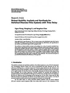
As the angular speed of the rotor increases, an instability of a purely mechanical origin is encountered in this periodic system. It is associated with a coupling between the motions of the blades in the plane of rotation of the rotor and lateral vibrations of the tower. If the blades are considered to be rigid bodies and the tower replaced by an equivalent spring-mass system, it is possible to find an analytical solution of the problem: the governing equations with periodic coefficients are transformed to a set of equations with constant coefficients using a Fourier transformation, and classical methods are then used to predict linearized stability. Next, the proposed approach to stability analysis was applied to the complete structural dynamics model at various rotor speeds, Ω. A small perturbation, in the form of a triangular impulsive moment (total duration: 0.05 sec; maximum amplitude: 100 kN·m) acting at the lag hinge of the first blade, was used to excite the system. The autoregressive method was used to assess stability based on the time histories of seven sensors: two tip transverse deflections of the tower, two root bending moments of the tower, and the three relative rotations of the blade lag hinges. The predicted system damping rates are shown in Fig. 7: the system is found to be unstable for Ω ∈ [9.4, 11.3] rad/sec. For reference, the analytical solution obtained from the approximate, rigid body model is also shown in the figure; although the damping rates predicted by the two models are slightly different, as expected, the predicted instability boundaries are in close agreement. Two additional simulations were performed by removing one or two of the lag hinge dampers; the results are also shown in Fig. 7. It is interesting to note that the loss of one or two dampers does not significantly alter the stability characteristics of the system. It should be noted here that while all the results presented for the UH-60 model were obtained based on the assumption of a linear system with constant coefficient, the results of the present example assumed the linear system to feature periodic coefficients.
Conclusions Linearized stability analysis methodologies that are applicable to comprehensive rotorcraft models were presented in this paper. The first contribution of this work is the development of two classes of closely related algorithms based on a partial Floquet and on an autoregressive approach, respectively.
AHS Log No. 1394
21
The common foundation of these approaches was emphasized. Second, the robustness of the proposed methodology was improved by using optimized signals that are derived from the proper orthogonal modes of the system, a set of orthogonal modes capturing the dominant motion of the system in an energy norm. Even for large systems, proper orthogonal modes can be effectively extracted from the very large set of data represented by the response of all degrees of freedom of the system using Lanczos’ algorithm. The proposed approaches are computationally inexpensive and consist of purely post processing steps that can be used with any comprehensive rotorcraft code or with experimental data. The singular value decomposition is systematically used as a means of dealing with noisy, highly redundant data sets. Unlike classical stability analysis methodologies, the linearization of the equations of motion of the system is not required. Application of the proposed methodology to system featuring nonlinear components was demonstrated.
References 1
Friedmann, P.P., “Numerical methods for determining the stability and response of periodic systems
with applications to helicopter rotor dynamics and aeroelasticity,” Computers and Mathematics with Applications, Vol. 12A, (1), 1986, pp. 131–148. 2
Gaonkar, G.H., and Peters, D.A., “Review of Floquet theory in stability and response analysis of
dynamic systems with periodic coefficients,” R.L. Bisplinghoff Memorial Symposium Volume on Recent Trends in Aeroelasticity, Structures and Structural Dynamics, Feb 6-7, 1986, pp. 101–119. University Press of Florida, Gainesville, 1986. 3
Subramanian, S., Gaonkar, G.H., Nagabhushanam, J., and Nakadi, R.N., “Parallel computing con-
cepts and methods for Floquet analysis of helicopter trim and stability,” Journal of the American Helicopter Society, Vol. 41, (4), 1996, pp. 370–382. 4
Johnson. W., “Rotorcraft dynamics models for a comprehensive analysis,” American Helicopter
Society 42nd Annual Forum Proceedings, Washington, D.C., May 1998. 5
Bauchau, O.A., Bottasso, C.L., and Nikishkov, Y.G., “Modeling rotorcraft dynamics with finite
22
OLIVIER A. BAUCHAU
JOURNAL OF THE AMERICAN HELICOPTER SOCIETY
element multibody procedures,” Mathematical and Computer Modeling, Vol. 33, (10-11), 2001, pp. 1113–1137. 6
Bauchau, O.A., and Wang, J.L., “Stability analysis of complex multibody systems,” Journal of
Computational and Nonlinear Dynamics, Vol. 1, (1), 2006, pp. 71–80. 7
Bauchau, O.A., and Wang, J.L., “Efficient and robust approaches to the stability analysis of large
multibody systems,” ASME Journal of Computational and Nonlinear Dynamics, 2007. To appear. 8
Murphy, K.D., Bayly, P.V., Virgin, L.N., and Gottwald, J.A., “Measuring the stability of periodic
attractors using perturbation induced transients: Applications to two nonlinear oscillators,” Journal of Sound and Vibration, Vol. 172, (1), 1994, pp. 85–102. 9
Trickey, S.T., Virgin, L.N., and Dowell, E.H., “The stability of limit cycle oscillations in a nonlinear
aeroelastic system,” Proceedings of the Royal Society of London, Vol. 458, (2025), 2002, pp. 2203–2226. 10
Quaranta, G., Mantegazza, P., and Masarati, P., “Assessing the local stability of periodic motions
for large multibody non-linear systems using proper orthogonal decomposition,” Journal of Sound and Vibration, Vol. 271, (3-5), 2004, pp. 1015–1038. 11
Lathrop, D.P, and Kostelich, E.J., “Characterization of an experimental strange attractor by periodic
orbits,” Physical Review A, Vol. 40, (7), 1989, pp. 4028–4031. 12
Antoulas, A.C., Sorensen, D.C., and Gugercin, S., “A survey of model reduction methods for large
scale systems,” Contemporary Mathematics, AMS Publication, Vol. 280, 2001, pp. 193–219. 13
Ho, B., and Kalman, R., “Efficient construction of linear state variable models from input/output
functions,” Regelungstechnik, Vol. 14, 1966, pp. 545–548. 14
Juang, J.N., and Pappa, R.S., “An eigensystem realization algorithm for modal parameter identifica-
tion and model reduction,” Journal of Guidance, Control, and Dynamics, Vol. 8, (5), 1985, pp. 620–627. 15
Moore, B.C., “Principal component analysis in linear systems: Controllability, observability, and
model reduction,” IEEE Transaction on Automatic Control, Vol. AC-26, (1), 1981, pp. 17–32. 16
Gugercin, S., and Antoulas, A.C., “A survey of model reduction by balanced truncation and some
new results,” International Journal of Control, Vol. 77, (8), 2004, pp. 748–766. 17
Durbin, J., “Efficient estimation of parameter in moving average models,” Biometrica, Vol. 46, (3-4),
1959, pp. 306–316.
AHS Log No. 1394
23
18
Ewins, D.J., “Modal testing: theory and practice,” Wiley, New York, 1984. Chapter 4.
19
Kay, S.M., and Nagesha, V., “Maximum likelihood estimation of signals in autoregressive noise,”
IEEE Transactions on Signal Processing, Vol. 42, (1), 1994, pp. 88–101. 20
Gautier, P.E., Gontier, C., and Smail, M., “Robustness of an ARMA identification method for modal
analysis of mechanical systems in the presence of noise,” Journal of Sound and Vibration, Vol. 179, (2), 1995, pp. 227–242. 21
Glover, K., “All optimal Hankel-norm approximations of linear multivariable systems and their L
inf-error bounds,” International Journal of Control, Vol. 39, (4), 1984, pp. 1115–1193. 22
Shin, K., Hammon, J.K., and White, P.R., “Iterative SVD method for noise reduction of low-
dimensional chaotic time series,” Mechanical Systems and Signal Processing, Vol. 13, (1), 1999, pp. 115–124. 23
Pearson, K., “On lines and planes of closest fit to points in space,” Philosophical Magazine, Vol. 2,
(11), 1901, pp. 609–629. 24
Lieu, T., Farhat, C., and Lesoinne, M., “Reduced-order fluid/structure modeling of a complete aircraft
configuration,” Computer Methods in Applied Mechanics and Engineering, Vol. 195, (41-43), 2006, PP. 5730-5742. 25
Bialecki, R.A., Kassab, A.J., and Fic, A., “Proper orthogonal decomposition and modal analysis
for acceleration of transient FEM thermal analysis,” International Journal for Numerical Methods in Engineering, Vol. 62, (6), 2005, pp. 774–797. 26
Lall, S., Marsden, J.E., and Glava´ski, S., “A subspace approach to balanced truncation for model
reduction of nonlinear control systems,” International Journal of Robust and Nonlinear Control, Vol. 12, (5), 2002, pp. 519–535. 27
Feeny, B.F., and Kappagantu, R., “On the physical interpretation of proper orthogonal modes in
vibrations,” Journal of Sound and Vibration, Vol. 211, (4), 1998, pp. 607–611. 28
Azeez, M.F.A. and Vakakis, A.F., “Proper orthogonal decomposition (POD) of a class of vibroimpact
oscillations,” Journal of Sound and Vibration, Vol. 240, (5), 2001, pp. 859–889. 29
Hochstadt, H., Differential Equations. Dover Publications, Inc., New York, 1964. Chapter 6.
24
OLIVIER A. BAUCHAU 30
JOURNAL OF THE AMERICAN HELICOPTER SOCIETY
Nayfeh, A.H., and Mook, D.T., Nonlinear Oscillations. John Wiley & Sons, New York, 1979.
Chapter 5. 31
Bauchau, O.A., and Nikishkov, Y.G., “An implicit Floquet analysis for rotorcraft stability evaluation,”
Journal of the American Helicopter Society, Vol. 46, (3), 2001, pp. 200–209. 32
O.A. Bauchau and Y.G. Nikishkov. An implicit transition matrix approach to stability analysis of
flexible multibody systems. Multibody System Dynamics, Vol. 5, (3), 2001, pp. 279–301. 33
Wang X., and Peters, D.A., “Floquet analysis in the absence of complete information on states
and perturbations,” Proceedings of the Seventh International Workshop on Dynamics and Aeroelasticity Stability Modeling, St. Louis, October 14-16, 1997, pp. 237–248. 34
Peters, D.A., and Wang, X, “Generalized floquet theory for analysis of numerical or experimental
rotor response data,” Proceedings of the 24th European Rotorcraft Forum, Marseilles, France, September 1998. 35
Golub, G.H., and Van Loan, C.F., Matrix Computations. The Johns Hopkins University Press,
Baltimore, second edition, 1989. Chapter 8. 36
Lardies, J., “Analysis of multivariate autoregressive process,” Mechanical Systems and Signal Pro-
cessing, Vol. 10, (6), 1996, pp. 747–761. 37
Fierro, R.D., and Jiang, E.P., “Lanczos and the riemannian SVD in information retrieval applica-
tions,” Numerical Linear Algebra With Applications, Vol. 12, (4), 2005, pp. 355–372. 38
Kokiopoulou, E., Bekas, C., and Gallopoulos, E., “Computing smallest singular triplets with im-
plicitly restarted Lanczos bidiagonalization,” Applied Numerical Mathematics, Vol. 49, (1), 2004, pp. 39–61. 39
Bousman W.G., and Maier, T., “An investigation of helicopter rotor blade flap vibratory loads,”
American Helicopter Society 48th Annual Forum Proceedings, Washington, D.C., June 3-5 1992, pp. 977–999. 40
Peters, D.A., Karunamoorthy, S., and Cao, W.M., “Finite state induced flow models. Part I: Two-
dimensional thin airfoil,” Journal of Aircraft, Vol. 32, (2), 1995, pp. 313–322. 41
Peters, D.A., and He, C.J., “Finite state induced flow models. Part II: Three-dimensional rotor disk,”
Journal of Aircraft, Vol. 32, (2), 1995, pp. 323–333.
AHS Log No. 1394 42
25
Bauchau, O.A., and Liu. H.Y., “On the modeling of hydraulic components in rotorcraft systems,”
Journal of the American Helicopter Society, Vol. 51, (2), 2006, pp. 175–184. 43
Bauchau, O.A., van Weddingen, Y., and Agarwal, S.,
“Semi-active Coulomb friction lead-lag
dampers,” Journal of the American Helicopter Society, 2008. Submitted for publication. 44
Stol, K., Bir, G., and Balas, M., “Linearized dynamics and operating modes of a simple wind turbine
model,” Proceedings of the 37th AIAA Aerospace Sciences Meeting and Exhibit, Reno, Nevada, Jan. 11-14, 1999, pp. 135–142. NICH Report No. 32548.
Appendix: The Singular Value Decomposition The present work requires the manipulation of large data sets that are highly redundant and noisy. The main tool for extracting reliable information from these data sets is the singular value decomposition (Ref. 35). The singular value decomposition of a real rectangular matrix S ∈ Rm×n , m > n, of rank n is · ¸ Σn×n T Sm×n = Um×n Γm×(m−n) (29) Vn×n , 0(m−n)×n where Σ = diag(σi ) is a unique diagonal matrix of nonnegative singular values σi ; [U Γ] an orthogonal matrix, implying U T U = I, ΓT Γ = I, U T Γ = 0 and ΓT U = 0; V an orthogonal matrix, implying V T V = V V T = I, and Γ forms the null space of S T , i.e. S T Γ = 0. The compact form of the singular value decomposition is S = U ΣV T . When dealing with highly redundant data sets, many of the singular values of S will be nearly zero. Typically, if the singular values are ordered in descending order, the following situation is encountered σ1 σ2 σr σr+1 σr+2 σn ≥ ≥ ... ≥ ≥ ≈ ≈ ≈ 0. σ1 σ1 σ1 σ1 σ1 σ1
(30)
In practice, this situation is met when σr+1 /σ1 < ε, i = r + 1, r + 2, . . . , n, where ε is a small number. In effect, it follows that rank(S) = r < n. Matrix S can now be approximated as S ≈ Sr = Ur Σr VrT , where matrices Ur and Vr consist of the first r columns of U and V , respectively, and Σr is the r × r principal minor of Σ; it can be shown that Sr is the rank r matrix that is closest to S in the Frobenius norm. This approximation is based on the selection of the small quantity, ε; a more physically meaningful criterion to
26
OLIVIER A. BAUCHAU
JOURNAL OF THE AMERICAN HELICOPTER SOCIETY
determine the rank of S is the following energy ratio criterion à r ! à n ! X X Er = σi / σi , i=1
(31)
i=1
that indicates the amount of energy captured in the retained modes as a fraction of the total amount of energy contained in the signal.
List of Tables 1
Identified frequencies, ωn [rad/sec], of rotor in forward flight at 158 knots. Case I: four sensors are used as input signals; case II: six proper orthogonal modes are used as inputs.
2
28
Identified damping rates, ζ [%], of rotor in forward flight at 158 knots. Case I: four sensors are used as input signals; case II: six proper orthogonal modes are used as inputs. . . . .
29
Table 1.
Identified frequencies, ωn [rad/sec], of rotor in forward flight at 158 knots. Case I: four sensors
are used as input signals; case II: six proper orthogonal modes are used as inputs. Case I:
sensors
Case II:
P.O.M.
Rank
Lead-lag
1st Flap
2nd Flap
Torsion
Lead-lag
1st Flap
2nd Flap
Torsion
12
7.06
29.97
73.97
111.91
7.00
30.13
75.75
115.79
18
7.08
29.69
75.32
116.58
7.08
29.87
76.66
113.51
24
7.04
29.65
76.19
113.40
7.00
29.60
75.85
113.56
32
7.11
29.63
75.85
113.09
7.02
29.45
76.76
113.28
40
7.09
29.54
76.43
113.71
7.02
29.62
77.14
114.32
48
7.07
29.56
77.04
113.64
7.01
29.63
77.46
114.25
60
7.09
29.58
76.91
112.81
7.01
29.58
76.40
113.89
mean
7.08
29.66
75.96
113.59
7.02
29.70
76.58
114.08
C.V.
0.31%
0.46%
1.29%
1.18%
0.38%
0.71%
0.76%
0.69%
Table 2.
Identified damping rates, ζ [%], of rotor in forward flight at 158 knots. Case I: four sensors are
used as input signals; case II: six proper orthogonal modes are used as inputs. Case I:
sensors
Case II:
P.O.M.
Rank
Lead-lag
1st Flap
2nd Flap
Torsion
Lead-lag
1st Flap
2nd Flap
Torsion
12
-9.18
-13.29
-7.13
-4.43
-9.40
-19.06
-9.12
-4.45
18
-9.14
-19.37
-9.12
-4.61
-8.78
-16.10
-8.16
-4.50
24
-9.47
-15.91
-8.07
-3.42
-9.52
-16.14
-8.57
-4.15
32
-9.07
-16.13
-9.01
-5.89
-9.61
-16.14
-8.60
-4.38
40
-9.14
-15.76
-8.23
-10.44
-9.49
-16.49
-8.24
-4.14
48
-9.19
-16.19
-8.04
-3.79
-9.59
-16.50
-8.89
-4.12
60
-9.15
-16.41
-8.32
-10.99
-9.51
-16.72
-9.99
-4.05
mean
-9.19
-16.15
-8.27
-6.23
-9.41
-16.73
-8.80
-4.26
C.V.
-1.31%
-10.16%
-7.47%
-47.09%
-2.84%
-5.82%
-6.58%
-3.96%
List of Figures 1
Schematic of the UH-60 rotor system. . . . . . . . . . . . . . . . . . . . . . . . . . . .
2
The frequencies and damping rates of the UH-60 rotor system. Lead-lag mode: (2); first flap mode: (¦); second flap mode: (?); torsion mode: (◦). . . . . . . . . . . . . . . . . .
3
31
32
Signals 1, 2 and 3: blade three-quarter transverse deflection, lead-lag deflection and twist, respectively. Signal 4: blade root flap angle. Original signal: solid line; reconstructed signal: dashed line. Forward flight speed of 158 knots. . . . . . . . . . . . . . . . . . .
4
33
Damping rate of the lead-lag mode as a function of normal force at the friction interface of the semi-active Coulomb friction damper. The damping rate of the hydraulic damper is given for reference. Forward flight at 156 knots . . . . . . . . . . . . . . . . . . . . . .
5
34
Signal synthesis of lead-lag damper stroke, friction damper for the normal force equal to 7500 lbs. For different rank number: r = 12, top figure; r = 84, middle figure; r = 96, bottom figure. Original signal: solid line; signal reconstruction: dashed line. . . . . . . .
35
6
Schematic of the wind turbine problem. . . . . . . . . . . . . . . . . . . . . . . . . . .
36
7
Damping in the wind turbine problem as a function of rotor angular speed. Analytical solution (2); all three dampers active (5); two dampers active only (♦); single damper active (4). . . . . . . . . . . . . . . . . . . . . . . . . . . . . . . . . . . . . . . . . . .
37
Fig. 1 Schematic of the UH-60 rotor system.
Frequency ω [rad/sec]
120 100 80 60 40 20 0
0
20
40
0
20
40
60
80
100
120
140
160
60
80
100
120
140
160
Damping rate ζ [%]
0
−5
−10
−15
−20
Forward speed [knots]
Fig. 2 The frequencies and damping rates of the UH-60 rotor system. Lead-lag mode: (2); first flap mode: (¦); second flap mode: (?); torsion mode: (◦).
Fig. 3 Signals 1, 2 and 3: blade three-quarter transverse deflection, lead-lag deflection and twist, respectively. Signal 4: blade root flap angle. Original signal: solid line; reconstructed signal: dashed line. Forward flight speed of 158 knots.
Fig. 4 Damping rate of the lead-lag mode as a function of normal force at the friction interface of the semi-active Coulomb friction damper. The damping rate of the hydraulic damper is given for reference. Forward flight at 156 knots
Time [sec]
Fig. 5 Signal synthesis of lead-lag damper stroke, friction damper for the normal force equal to 7500 lbs. For different rank number: r = 12, top figure; r = 84, middle figure; r = 96, bottom figure. Original signal: solid line; signal reconstruction: dashed line.
Fig. 6 Schematic of the wind turbine problem.
0.4
0.35
0.3
Damping [1/sec]
0.25
0.2
0.15
0.1
0.05
0
−0.05
−0.1
6
7
8
9
10
11
12
13
Angular Velocity [rad/sec]
Fig. 7 Damping in the wind turbine problem as a function of rotor angular speed. Analytical solution (2); all three dampers active (5); two dampers active only (♦); single damper active (4).