In a typical reinforcement learning (RL) setting details of the environment are ... functions to posteriors by observing samples from the MDP [4, 5]. Ghavamzadeh.
Efficient Uncertainty Propagation for Reinforcement Learning with Limited Data Alexander Hans1,2 and Steffen Udluft1
?
1- Siemens AG, Corporate Technology, Information & Communications, Learning Systems, Otto-Hahn-Ring 6, D-81739 Munich, Germany {alexander.hans.ext|steffen.udluft}@siemens.com 2- Ilmenau Technical University, Neuroinformatics and Cognitive Robotics Lab, P.O.Box 100565, D-98684 Ilmenau, Germany
Abstract. In a typical reinforcement learning (RL) setting details of the environment are not given explicitly but have to be estimated from observations. Most RL approaches only optimize the expected value. However, if the number of observations is limited considering expected values only can lead to false conclusions. Instead, it is crucial to also account for the estimator’s uncertainties. In this paper, we present a method to incorporate those uncertainties and propagate them to the conclusions. By being only approximate, the method is computationally feasible. Furthermore, we describe a Bayesian approach to design the estimators. Our experiments show that the method considerably increases the robustness of the derived policies compared to the standard approach. Key words: reinforcement learning, model-based, uncertainty, Bayesian modeling
1
Introduction
In reinforcement learning (RL) [12] one is concerned with finding a policy, i.e. a mapping from states to actions, that moves an agent optimally in an environment assumed to be a Markov decision process (MDP) M := (S, A, P, R) with a state space S, a set of possible actions A, the system dynamics, defined as probability distribution P : S × A × S → [0, 1], which gives the probability of reaching state s0 by executing action a in state s, and a reward function R : S × A × S → R, which determines the reward for a given transition. If the parameters of the MDP are known a priori, an optimal policy can be determined, e.g., using dynamic programming. Often, however, the MDP’s parameters are not known in advance. A common way of handling this situation is model-based RL, where one first estimates a model of the MDP from a number of observations and then finds an optimal policy w.r.t. that model. In general, such a policy will not be optimal w.r.t. the real MDP. Especially in case of a limited number of observations the estimated MDP has a high probability to differ from the real one substantially. In this case, it is in particular possible to derive a policy that will perform badly when applied to the real MDP. ?
The authors would like to thank the reviewers for very useful comments.
By incorporating the model estimators’ uncertainties into the determination of the policy it is possible to weaken this problem. In recent work by Schneegass et al. [10] uncertainty propagation (UP) was applied to the Bellman iteration to determine the Q-function’s [12] uncertainty and derive uncertainty incorporating policies. While the algorithm described in [10] provides significant advantages over methods not considering uncertainty, it adds a huge computational burden for updating the covariance matrix in each iteration. In this paper, we propose an algorithm called the diagonal approximation of uncertainty incorporating policy iteration (DUIPI) for discrete MDPs that represents an efficient way of using UP to incorporate the model’s uncertainty into the derived policy by only considering the diagonal of the covariance matrix. Only considering the diagonal neglects the correlations between the state-action pairs, which in fact are small for many RL problems, where on average different state-action pairs share only little probabilities to reach the same successor states. DUIPI is easier to implement and, most importantly, lies in the same complexity class as the standard Bellman iteration and is therefore computationally much cheaper than the method considering the full covariance matrix. Although some of the results obtained with DUIPI are not as good as those of the full-matrix method, the robustness of the resulting policies is increased considerably, compared to the standard Bellman iteration, which does not regard the uncertainty. In this context it furthermore is advisable to use Bayesian statistics to model the a posteriori distributions of the transition probabilities and rewards in order to access the estimators’ uncertainties properly. Additionally, it allows the specification of prior knowledge and the user’s belief. There have already been a number of contributions that consider uncertainties when estimating MDPs. E.g., the framework of robust MDPs has widely been studied (e.g., [8, 1]), in which one assumes that all uncertainties can only lie within a bounded set. One tries to find policies optimizing the worst case within that set, which often results in too conservative policies. Within the context of Bayesian RL, incorporation of prior knowledge about confidence and uncertainty directly into the approached policy is possible. E.g., Engel et al. applied Gaussian processes for policy evaluation by updating a prior distribution over value functions to posteriors by observing samples from the MDP [4, 5]. Ghavamzadeh and Engel presented additional Bayesian approaches to model-free RL [6, 7]. Using Gaussian processes inherently introduces a measure of uncertainty based on the number of samples. When dealing with model-based approaches, however, one starts with a natural local measure of the uncertainty of the transition probabilities and the rewards. In that context, related to the present paper is work by Delage and Mannor [3], who used convex optimization to solve the percentile problem and applied it to the exploration-exploitation trade-off. Model-based interval estimation (MBIE) was also used for efficient exploration by using local uncertainty to derive optimistic exploration policies, e.g., [11]. The remainder of the paper is organized as follows. In sec. 2 we describe how to incorporate knowledge of uncertainty into the Bellman iteration using
UP, sec. 3 presents ways of parameter estimation. Experiments and results are presented in sec. 4. Sec. 5 finishes the paper with a short conclusion.
2
Incorporation of Uncertainty
Our notion of uncertainty is concerned with the uncertainty that stems from the ignorance of the exact properties of the real MDP, as they are usually unknown and must be estimated from observations. With an increasing number of observations the uncertainty decreases; in the limit of an infinite number of observations of every possible transition the uncertainty vanishes as the true properties of the MDP are revealed. For a given number of observations the uncertainty depends on the inherent stochasticity of the MDP; if the MDP is known to be completely deterministic, one observation of a transition is sufficient to determine all properties of that transition; the more the MDP is stochastic, the more uncertainty will remain for a fixed number of observations. It is important to distinguish this uncertainty from an MDP’s inherent stochasticity. We want to use the knowledge of uncertainty to determine an optimal Qfunction Q∗ with its uncertainty σQ∗ . In a second step it is then possible to change the Bellman iteration to not only regard a Q-value but also its uncertainty, resulting in a policy that generally prefers actions that have a low probability of leading to an inferior long-term reward. 2.1
Determining the Q-Function’s Uncertainty
To obtain the Q-function’s uncertainty, we use the concept of uncertainty propagation (UP), also known as Gaussian error propagation (e.g., [2]), to propagate the uncertainties of the measurements, i.e., the transition probabilities and the rewards, to the conclusions, i.e., the Q-function and policy. The uncertainty of P � ∂f �2 (σxi )2 . The values f (x) with f : Rm → Rn is determined as (σf )2 = i ∂x i update step of the Bellman iteration, h i X ˆ a, s0 ) + γV m−1 (s0 ) , Pˆ (s0 |s, a) R(s, (1) Qm (s, a) := s0
can be regarded as a function of the estimated transition probabilities Pˆ and ˆ and the Q-function of the previous iteration Qm−1 (V m−1 is a subset rewards R, m−1 ), that yields the updated Q-function Qm . Applying UP to the Bellman of Q iteration, one obtains an update equation for the Q-function’s uncertainty: X X (σQm (s, a))2 := (DQQ )2 (σV m−1 (s0 ))2 + (DQP )2 (σ Pˆ (s0 |s, a))2 + s0
s0
X ˆ a, s0 ))2 , (DQR )2 (σ R(s, s0
ˆ a, s0 ) + γV m−1 (s0 ), DQR = Pˆ (s0 |s, a). DQQ = γ Pˆ (s0 |s, a), DQP = R(s,
(2)
V m and σV m have to be set depending on the desired type of the policy (stochastic or deterministic) and whether policy evaluation or policy iteration is performed. E.g., for policy evaluation of a stochastic policy π X V m (s) = π(a|s)Qm (s, a), (3) a
(σV m (s))2 =
X
π(a|s)2 (σQm (s, a))2 .
(4)
a
For policy iteration, according to the Bellman optimality equation and resulting in the Q-function Q∗ of an optimal policy, V m (s) = maxa Qm (s, a) and (σV m (s))2 = (σQm (s, arg maxa Qm (s, a)))2 . ˆ with their uncertainties σ Pˆ and σ R ˆ and Using the estimators Pˆ and R 0 0 starting with an initial Q-function Q and corresponding uncertainty σQ , e.g., Q0 := 0 and σQ0 := 0, through the update equations (1) and (2) the Q-function and corresponding uncertainty are updated in each iteration and converge to Qπ and σQπ for policy evaluation and Q∗ and σQ∗ for policy iteration. Q∗ and σQ∗ can be used to obtain the function Qu (s, a) = Q∗ (s, a) − ξσQ∗ (s, a),
(5)
specifying a performance limit which, when the policy π ∗ is applied to the real MDP, will be exceeded with probability Pr(Z(s, a) > Qu (s, a)) = F (ξ), where Z is the (unknown) Q-function of π ∗ for the real MDP. F (ξ) depends on the distribution class of Q. E.g., if Q is normally distributed, F is the distribution function of the standard normal distribution. Note that a policy based on Qu , i.e. πu (s) = arg maxa Qu (s, a), does not in general improve the performance limit, as Qu considers the uncertainty only for one step. In general, Qu does not represent πu ’s Q-function, which poses an inconsistency. To use the knowledge of uncertainty for maximizing the performance limit (as opposed to the expectation), the uncertainty needs to be incorporated into the policy-improvement step. 2.2
Uncertainty-Aware Policy Iteration
The policy-improvement step is contained within the Bellman optimality equation as maxa Qm (s, a). Alternatively, determining the optimal policy in each iteration as ∀s : π m (s) := arg max Qm (s, a) (6) a
and then updating the Q-function using this policy, i.e., h i X ˆ a, s0 ) + γQm−1 (s0 , π m−1 (s)) , ∀s, a : Qm (s, a) := Pˆ (s0 |s, a) R(s,
(7)
s0
yields the same solution. To determine a so-called certain- or ξ-optimal policy that maximizes the performance limit for a given ξ, the update of the policy must not choose the optimal action w.r.t. to the maximum over the Q-values
of a particular state but the maximum over the Q-values minus their weighted uncertainty: ∀s : π m (s) := arg max [Qm (s, a) − ξσQm (s, a)] . a
(8)
In each iteration, the uncertainty σQm has to be updated as described in sec. 2.1, setting V m and σV m as for deterministic policy evaluation. The parameter ξ controls the influence of the uncertainty on the policy. Choosing a positive ξ yields uncertainty avoiding policies, with increasing ξ a worst-case optimal policy is approached. A negative ξ results in uncertainty seeking behavior. 2.3
Non-Convergence of DUIPI for Deterministic Policy Iteration
While it has been shown that conventional policy iteration in the framework of MDPs is guaranteed to converge to a deterministic policy [9], for ξ-optimal policies derived by the algorithm presented in sec. 2.2 this is not necessarily the case. When considering a Q-value’s uncertainty for action selection, there are two effects that contribute to an oscillation of the policy and consequently non-convergence of the corresponding Q-function. First, there is the effect mentioned in [10] of a bias on ξσQ(s, π(s)) being larger than ξσQ(s, a), a 6= π(s), if π is the evaluated policy and ξ > 0. DUIPI is not affected by this problem due to the ignorance of covariances between Q and R. Second, there is another effect (by which DUIPI is affected) causing an oscillation when there is a certain constellation of Q-values and corresponding uncertainties of concurring actions. Consider two actions a1 and a2 in a state s with similar Q-values but different uncertainties, a1 having an only slightly higher Q-value but a larger uncertainty. The uncertainty-aware policy improvement step would alter π m to choose a2 , the action with the smaller uncertainty. However, the fact that this action is inferior might only become obvious in the next iteration when the value function is updated for the altered π m (and now implying the choice of a2 in s). In the following policy improvement step the policy will be changed back to choose a1 in s, since now the Q-function reflects the inferiority of a2 . After the next update of the Q-function, the values for both actions will be similar again, because now the value function implies the choice of a1 and the bad effect of a2 affects Q(s, a2 ) only once. 2.4
Risk-Reduction by Diversification through Stochastic Policies
With stochastic policies it is possible to construct an update-scheme that is guaranteed to converge, thus solving the problem of non-convergence. Moreover, it is intuitively clear that for ξ > 0 ξ-optimal policies should be stochastic as one tries to decrease the risk of obtaining a low long-term reward (because the wrong MDP has been estimated) by diversification. The resulting algorithm initializes the policy with equiprobable actions. In each iteration, the probability of the best action according to Qm u (equation (5))
is increased by 1/m, m being the current iteration, while the probabilities of all other actions are decreased accordingly: min(π m−1 (a|s) + 1/m, 1), if a = aQm−1 (s) u m (s))−1/m,0) ∀s, a : π (a|s) := max(1−π(s,aQm−1 u π m−1 (a|s), otherwise 1−π(s,a m−1 (s)) Qu
(9) aQum−1 (s) denotes the best action according to Qm−1 , i.e. aQm−1 (s) = u u arg maxa Qm−1 (s, a)−ξσQm−1 (s, a). Due to the harmonically decreasing change rate convergence as well as reachability of all possible policies are ensured.
3
Modeling of Estimators and their Uncertainty
There are several ways of modeling the estimators for the transition probabilities P and the reward R. In the following we will present the frequentist approach using relative frequency as well as a Bayesian approach. 3.1
Frequentist Estimation
In the frequentist paradigm the relative frequency is used as the expected transition probability. The uncertainty of the according multinomial distribution is assumed to be (σ Pˆ (s0 |s, a))2 =
Pˆ (s0 |s, a)(1 − Pˆ (s0 |s, a)) , nsa − 1
(10)
where nsa denotes the number of observed transitions from (s, a). Using the same concept for the rewards and assuming a normal distribution, the mean of all observed rewards of a transition (s, a, s0 ) is used as reward expectation, their uncertainties are ˆ a, s0 ))2 = (σ R(s,
ˆ a, s0 )) var(R(s, , nsas0 − 1
(11)
with nsas0 being the number of observed transitions (s, a, s0 ). Although the estimation of the transition probabilities using relative frequency usually leads to good results in practice, the corresponding uncertainty estimation is problematic if there are only a few observations, because in that case the uncertainties are often underestimated. For instance, if a specific transition is observed twice out of two tries (nsas0 = nsa = 2), its uncertainty σ Pˆ (s0 |s, a) = 0. 3.2
Bayesian Estimation
Assuming all transitions from different state-action pairs to be independent of each other and the rewards, the transitions can be modeled as multinomial distributions. In a Bayesian setting, where one assumes a prior distribution over the
parameter space P (sk |si , aj ) for given i and j, the Dirichlet distribution with density Pr(P (s1 |si , aj ), . . . , P (s|S| |si , aj ))αij1 ,...,αij|S| = Γ(αij )
|S| Y
Q|S|
k=1 Γ(αijk ) k=1
αij =
P|S|
k=1 αijk , is P|S| d = k=1 αij
P (sk |si , aj )αijk −1 ,
(12)
d a conjugate prior with posterior parameters αijk = αijk +
d nsi aj sk , αijk . Choosing the expectation of the posterior distribution d d as the estimator, i.e. Pˆ (sk |si , aj ) = αijk /αij , the uncertainty of Pˆ is
(σ Pˆ (sk |si , sj ))2 =
d d d αijk (αi,j − αijk ) d )2 (αd + 1) (αij ij
.
(13)
Note that αi = 0 results in a prior that leads to the same estimates and slightly lower uncertainties compared to the frequentist modeling of sec. 3.1. On the other hand, setting αi = 1 leads to a flat, maximum entropy prior that assumes all transitions from a state to all other states equally probable. Both settings, αi = 0 and αi = 1, represent extremes that we believe are unreasonable for most applications. Instead, we model our prior belief by setting m αi = |S| , where m is the average number of expected successor states of all stateaction pairs and |S| is the total number of states. This choice of αi realizes an approximation of a maximum entropy prior over a subset of the state space with a size of m states. This way most of the probability is “distributed” among any subset of m states that have actually been observed, the probability of all other (not observed) successor states becomes very low. Compared to the maximum entropy prior with αi = 1 one needs only a few observations for the actually observed successor states to be much more probable than not observed ones. At the same time, the estimation of the uncertainty is not as extreme as the frequentist one, since having made the same observation twice does not cause the uncertainty to become zero. Estimating m from the observations can easily be added.
4
Experiments
We conducted experiments with DUIPI as presented here and the full-matrix algorithm using the frequentist as well as the Bayesian estimators described in the previous section.1 4.1
Benchmark: Wet-Chicken 2D
The benchmark problem used was Wet-Chicken 2D, a two-dimensional version of the original Wet-Chicken benchmark [13]. In the original setting a canoeist 1
Source code for the benchmark problem as well as a DUIPI implementation is available at http://ahans.de/publications/icann2009/.
Wet−Chicken 2D 10x10
Wet−Chicken 2D 20x20 15 average reward
average reward
7
6
5
4 3
4
10
10 # observations
5
10
10
5 3 10
4
5
10
10
6
10
# observations
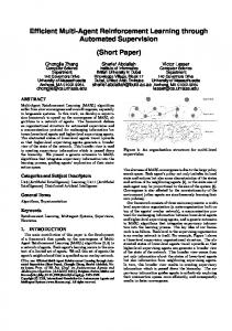
Fig. 1. Performance of policies generated using standard policy iteration (‘•’ marks), DUIPI (black lines), and the full-matrix method [10] (gray lines). ξ = 0.5 is indicated by ‘×’ marks, ξ = 1 by ‘+’ marks. Solid lines represent policies generated using frequentist estimators, dashed lines represent policies generated using Bayesian estimation.
paddles on a one-dimensional river with length l and flow velocity v = 1. At position x = l of the river there is a waterfall. Starting at position x = 0 the canoeist has to try to get as near as possible to the waterfall without falling down. If he falls down, he has to restart at position x = 0. The reward increases linearly with the proximity to the waterfall and is given by r = x. The canoeist has the possibility to drift (x−0+v = x+1), to hold the position (x−1+v = x), or to paddle back (x − 2 + v = x − 1). River turbulence of size s = 2.5 causes the state transitions to be stochastic. Thus, after having applied the canoeist’s action to his position (also considering the flow of the river), the new position is finally given by x0 = x + n, where n ∈ [−s, s] is a uniformly distributed random value. For the two-dimensional version the river is extended by a width w. Accordingly, there are two additional actions available to the canoeist, one to move the canoe to the left and one to move it to the right by one unit. The position of the canoeist is now denoted by (x, y), the (re-)starting position is (0, 0). The velocity of the flow v and the amount of turbulence s depend on y: v = 3y/w and s = 3.5 − v. In the discrete problem setting, which we use here, x and y are always rounded to the next integer value. While on the left edge of the river the flow velocity is zero, the amount of turbulence is maximal; on the right edge there is no turbulence (in the discrete setting), but the velocity is too high to paddle back. 4.2
Results
We performed experiments with a river size of 10x10 (100 states) and 20x20 (400 states). For both settings a fixed number of observations was generated using random exploration. The observations were used as input to generate policies using the different algorithms. The discount factor was chosen as γ = 0.95. Each resulting policy was evaluated over 100 episodes with 1000 steps each. The results are summarized in fig. 1 (averaged over 100 trials). For clarity only the results of stochastic policies are shown (except for ξ = 0, i.e., standard policy iteration), they performed better than the deterministic ones in all experiments. Usually a method like DUIPI aims at quantile optimization, i.e., reducing the
7
600
6
Wet−Chicken 2D 10x10 0.1−quantile & average reward
reward
number of policies
Wet−Chicken 2D 10x10 Policies from 4x10⁴ observations 800
400
5
200 4 0
5
5.5
6 6.5 average reward
7
3
10
4
10 # observations
5
10
Fig. 2. Left: histograms of average rewards of 104 policies with ξ = 0 (solid), ξ = 1 (dashed), and ξ = 2 (dotted). For the generation of each policy 4 × 10⁴ observations were used. Right: average (solid) and 0.1-quantile (dashed) average rewards of policies with ξ = 0 (‘•’ marks), ξ = 0.5 (‘×’ marks), and ξ = 1 (‘+’ marks).
probability of generating very poor policies at the expense of a lower expected average reward. However, in some cases it is even possible to increase the expected performance, when the MDP exhibits states that are rarely visited but potentially result in a high reward. For Wet-Chicken states near the waterfall have those characteristics. An uncertainty unaware policy would try to reach those states if there are observations leading to the conclusion that the probability of falling down is low, which in fact is high. In [10] this is reported as “border-phenomenon”, which by our more general explanation is included. Due to this effect it is possible to increase the average performance using uncertainty aware methods for policy generation, which can be seen from the figure. For small numbers of observations and high ξ-values DUIPI performs worse as in those situations the action selection in the iteration is dominated by the uncertainty of the Q-values and not the Q-values themselves. This leads to a preference of actions with low uncertainty, the Q-values play only a minor role. This effect is increased by the fact that due to random exploration most observations are near the beginning of the river, where the immediate reward is low. Using a more intelligent exploration scheme could help to overcome this problem. Due to the large computational and memory requirements the full-matrix method could not be applied to the problem with river size 20x20. Moreover, results of the full-matrix version with Bayesian estimation are not shown as they would not have been distinguishable in the figure. Fig. 2 compares uncertainty aware and unaware methods. Considering the uncertainty reduces the amount of poor policies and even increases the expected performance (ξ = 0.5). Setting ξ = 1 results in an even lower probability for poor policies at the expense of a lower expected average reward. Table 1. Computation times to generate a policy using a single core of an Intel Core 2 Quad Q9550 processor. method Wet-Chicken 5x5 Wet-Chicken 10x10 Wet-Chicken 20x20 full-matrix 5.61 s 1.1 × 10³ s — DUIPI 0.002 s 0.034 s 1.61 s
5
Conclusion
In this paper, we presented DUIPI, a computationally very feasible algorithm for incorporation of uncertainty into the Bellman iteration. It only considers the diagonal of the covariance matrix encoding the covariance. While this causes the algorithm to be only approximate, it also decreases its complexity, decreasing the computational requirements by orders of magnitude. Moreover, we proposed a Bayesian parameter estimation that incorporates prior knowledge about the number of successor states. Our experiments show that DUIPI increases the robustness and performance of policies generated for MDPs whose exact parameters are unknown and estimated from only a fixed set of observations. In industrial applications observations are often expensive and arbitrary exploration not possible, we therefore believe that for those applications knowledge of uncertainty is crucial. Future work will consider application of UP to RL algorithms involving function approximation and utilizing knowledge of uncertainty for efficient exploration.
References 1. G. Calafiore and L. El Ghaoui. On distributionally robust chance-constrained linear programs. In Optimization Theory and Applications, 2006. 2. G. D’Agostini. Bayesian Reasoning in Data Analysis: A Critical Introduction. World Scientific Publishing, 2003. 3. E. Delage and S. Mannor. Percentile optimization in uncertain Markov decision processes with application to efficient exploration. In Proc. of the Int. Conf. on Machine Learning, 2007. 4. Y. Engel, S. Mannor, and R. Meir. Bayes meets Bellman: the Gaussian process approach to temporal difference learning. In Proc. of the Int. Conf. on Machine Learning, 2003. 5. Y. Engel, S. Mannor, and R. Meir. Reinforcement learning with Gaussian processes. In Proc. of the Int. Conf. on Machine Learning, 2005. 6. M. Ghavamzadeh and Y. Engel. Bayesian policy gradient algorithms. In Advances in Neural Information Processing Systems, 2006. 7. M. Ghavamzadeh and Y. Engel. Bayesian actor-critic algorithms. In Proc. of the Int. Conf. on Machine Learning, 2007. 8. A. Nilim and L. El Ghaoui. Robustness in Markov decision problems with uncertain transition matrices. In Advances in Neural Information Processing Systems, 2003. 9. M.L. Puterman. Markov Decision Processes: Discrete Stochastic Dynamic Programming. John Wiley & Sons Canada, Ltd., 1994. 10. D. Schneegass, S. Udluft, and T. Martinetz. Uncertainty propagation for quality assurance in reinforcement learning. In Proc. of the Int. Joint Conf. on Neural Networks, 2008. 11. A.L. Strehl and M.L. Littman. An empirical evaluation of interval estimation for markov decision processes. In 16th IEEE Int. Conf. on Tools with Artificial Intelligence, pages 128–135, 2004. 12. R.S. Sutton and A.G. Barto. Reinforcement Learning: An Introduction. MIT Press, 1998. 13. V. Tresp. The wet game of chicken. Siemens AG, CT IC 4, Technical Report, 1994.