Electrocardiogram Baseline Removal Using Wavelet Approximations David Cuesta-Frau1, Daniel Novák2, Vladimir Eck2, Juan C. Pérez-Cortés 1, Gabriela Andreu-García 1 1 ( ) Department of System Informatics and Computers, Polytechnic University of Valencia, Valencia (Spain). (2)Department of Cybernetics, Czech Technical University in Prague, Prague, (Czech Republic). e-mail:
[email protected] Summary In this paper, a method to reduce the baseline wandering of an electrocardiogram signal is presented. The method described is based on wavelet approximation of the whole signal. The main advantage of this method, compared with others, is the fact that this is a non-supervised method, allowing the process to be used in an off-line automatic analysis of electrocardiograms. Moreover, the results are as accurate as those obtained with other methods, but with much less effort. Introduction One of the first stages applied in the preprocessing of electrocardiogram signals (e.s.) is the removal of baseline wandering. This interference appears in the acquisition stage due to different sources: patient movement, breathing, physical exercise, electrode contact, etc. Baseline wandering can make inspection of e.s. difficult, because some features can be masked by it. Moreover, in automatic inspection systems, other processing tasks such as wave detection, signal classification, etc. can be affected. It is, therefore, of importance to reduce as much as possible its effect. Some methods have been presented to achieve this goal, each one with advantages and disadvantages. For example, in [1,2] a method using cubic splines and curve approximation are presented. The results obtained with this method are good, but it needs the coordinates of baseline points to estimate it. Other methods such as [3,4] use signal
processing techniques, offering not so good results but which have been obtained more easily. In [5], a comparative study of some methods is presented. Usually, the application of these methods is only suitable in particular cases, with known conditions. In this study, a more general method is developed, without need of interaction with the user, and offering acceptable results. Materials and Methods Nowadays, wavelets constitute an important and fairly new tool for signal processing. Their main feature is their timefrequency analysis capability using a single transformation, which makes it useful in applications such as signal denoising, wave detection, data compression, feature extraction, etc [6]. There are many techniques based on Wavelets theory, such as Wavelets packets, Wavelets approximation and decomposition, Discrete and Continuous Wavelet Transform, etc. In this study, the Wavelet approximation of signals is applied, as the tool to obtain a good approximation of the e.s. baseline, since both are low frequency signals. This approximation is based on the signal decomposition in two parts, details or high frequency components, an the approximation itself, or low frequency components. These components are obtained from the signal comparison to some wavelets functions, scaled and translated, which constitute the base of the transformation [6]. Nevertheless, to obtain good results, the level of such approximation must be defined. Namely, the degree of accuracy of
the approximation. Otherwise, there will be an over-fitting effect in the baseline approximation due to an overly low level, as is shown in figure 1, or to the contrary, with a poor approximation due to an overly high level.
120
100
80
60
40
20
0
120
-20
100
-40
80
-60
60
7.8
7.9
8
8.1
8.2
8.3
8.4
8.5
8.6
8.7
8.8 x 10 4
Figure 2. Suitable approximation of the baseline using Wavelets. The level used is correct.
40
20
0
- 20
Results - 40
- 60
7.3
7.4
7.5
7.6
7.7
7.8
7.9 4
Figure 1. Over-fitting using Wavelet approximation. The level used is too low and then high-frequency features are also approximated.
The best level depends on the amplitude and main spectrum distribution of the baseline interference. In this study, a method to automatically ascertain the best level is also presented, which makes the process unsupervised. This method is based on measures of the resulting signal variance and on spectrum energy dispersion of the approximation. In order to eliminate or reduce the baseline wandering, the approximation found must have a narrow spectrum, as such interferences are usually almost pure sinusoids. Besides, the variance of the resulting signal should be as low as possible, since the approximation must not have high frequency components such as peaks following R waves, and so, the final signal must be quite flat. Once the level is obtained, the wavelet approximation is calculated, and then, it is subtracted from the signal. Consequently, the baseline wander of this signal is greatly reduced. The whole process is carried out without user intervention, which is an advantage compared with other more traditional methods. For example, in figure 2, a good baseline approximation using wavelets is shown.
The process described in this study has been applied to signals with a synthetic baseline wander, given by combined sinusoids. These sinusoids have been generated for a frequency range from 0.5Hz to 5Hz, in steps of 0.5Hz. Real signals from our database with baseline wandering have been tested, and also signals with the synthetic baseline wander described above. In both cases, the level of approximation obtained is such that the error of the resulting signal, after baseline suppression, is minimal. In order to obtain the approximation, some wavelets have been tested. After the experiments, such wavelets offering a lower level of approximation have been finally applied. Such wavelets are based on the Daubechies family [6]. In figures 3 and 4, featuring two kinds of results, the level calculations are shown. The functions plotted correspond to the error obtained after baseline wander removal, variance, and spectrum dispersion. It can be seen how the intersection points coincide with the level corresponding to the minimum error (dotted line). In figure 3, the intersection point corresponds exactly to level 8. It can be seen how the approximation dispersion is higher before and after that point. The resulting signal variance, also increases greatly after that point. The error, calculated from the difference between the ideal signal without baseline wandering and the signal obtained, is also greater before
and after that point, which shows the method is suitable for this task. 2
1.5
Dispersion 1
Variance
0.5
Error
0
-0.5
-1 6
6.5
7.5
7
8.5
8
9.5
10
10.5
11
9
Figure 3. Level approximation detection using variance and spectrum dispersion (x axis). The intersection point coincides with the minimum error.
In figure 4, the same functions are plotted, with similar results. Nevertheless, the intersection point is not situated in an integer level of decomposition, which happens in some cases. Anyway, the final level used is obtained from the nearest integer value, which is 8 in this case. 2
1.5
Dispersion
Variance
1
0.5
Error
0
-0.5
-1
6
6.5
7.5
7
8.5
8
9.5
10
10.5
11
9
Figure 4. Level approximation detection using variance and spectrum dispersion. The intersection point is approximated to the nearest integer to ascertain the level.
Discussion and Conclusion The method presented allows the offline removal of the baseline wandering without need of preprocessing or baseline points selection, which makes its use easier than other methods. Besides, it is not affected by signal noise because details, where the noise is included, are not used in the calculations.
Another advantage is the possibility of applying this approximation to a wide range of baseline wander fundamental frequency, because the level is automatically adapted, according to the dispersion of the approximation and variance of the resulting signal. The disadvantage of this method is the fact that one has to calculate some approximations to find the best one, although this can be done quite fast on most computers. Nevertheless, further work must be done in order to improve the results when the baseline bandwidth is wide, since the wavelet approximation covers only a narrow bandwidth. Some baselines based on sinc or chirp signals will be studied, including other sources of real signals with baseline wandering, such as MIT database. References [1] Meyer, C.R. ; Keiser, H.N., “Electrocardiogram Baseline Noise Estimation and Removal Using Cubic Splines and State-Space Computational Techniques”, Computers and Biomedical Research, vol. 10, pp 459-470, 1977. [2] Outram, N.J. et al, “Techniques for optimal enhancement and feature extraction of fetal electrocardiogram”, IEE Proc.-Sci. Meas. Technol., vol 142, no. 6, pp 482-489, 1995. [3] Van Alsté, J.A.;Schilder, T.S., “Removal of Base-Line Wander and Power-Line Interference from the ECG by an Efficient FIR Filter with a Reduced Number of Taps. IEEE Transactions on Biomedical Engineering, vol. 32, no. 12, December 1995. [4] Sörnmo, L. ,”Time-varying digital filtering of ECG baseline wander”. Medical & Biological Engineering & Computing, September 1993. [5] Royo, M.P.; Laguna P., “ECG Baseline Wandering Removal: A Comparative Study” (Spanish), XVI Annual Conference of the Spanish Society of Biomedical Engineering, CASEIB’98, Valencia (Spain), 1998. [6] Graps. A., “An Introduction to Wavelets”, IEEE Computational Science and Engineering, vol. 2, no. 2,1995.