A system of beam position monitors was designed, built, and commissioned in ...... spontaneous radiation bandwidth then this radiation is not amplified in the ...
Electron Beam Diagnostic at the ELBE Free Electron Laser
Dissertation zur Erlangung des akademischen Grades Doctor rerum naturalium (Dr. rer. nat.)
vorgelegt der Fakultät Mathematik und Naturwissenschaften der Technischen Universität Dresden
von Pavel Evtushenko, Magister der Physik geboren am 15. April 1975 in Berdsk, Russland
Contents Introduction....................................................................................................................1 Chapter 1 Fundamentals of FEL operation....................................................................3 1.1
Introduction....................................................................................................3
1.2
Electron trajectory in the undulator ...............................................................4
1.3
Spontaneous emission....................................................................................6
1.4
Stimulated emission .......................................................................................8
1.5
FEL gain.......................................................................................................11
1.6
Electron beam quality requirements ............................................................16
1.7
Conclusion ...................................................................................................19
Chapter 2 Transverse emittance...................................................................................20 2.1
Introduction..................................................................................................20
2.2
Phase space and emittance ...........................................................................20
2.3
Beam transport in linear approximation ......................................................24
2.4
Quadrupole scan emittance measurements ..................................................26
2.5
Beam envelope analysis...............................................................................33
2.6
Multislit emittance measurements in the ELBE injector .............................36
2.7
Conclusion ...................................................................................................42
Chapter 3 Bunch length measurements........................................................................43 3.1
Introduction..................................................................................................43
3.2
Bunch length evolution at ELBE .................................................................44
3.3
Bunch length measurements in the injector .................................................47
3.4
The method of bunch length measurement using coherent transition
radiation ...............................................................................................................50
ii
3.4.1
Transition radiation from a single charged particle .............................50
3.4.2
Transition radiation of an electron bunch ............................................51
3.4.3
The Martin-Puplett interferometer.......................................................54
3.5
Experimental setup for the CTR measurements ..........................................56
3.6
Experimental results.....................................................................................57
3.6.1 Linearity of the detectors ............................................................................57 3.6.2 Initial data evaluation..................................................................................59 3.6.3 Bunch length reconstruction .......................................................................61 3.6.4 Bunch length minimization.........................................................................63 3.7
Conclusion ...................................................................................................65
Chapter 4 Beam position monitor system....................................................................66 4.1
Motivation....................................................................................................66
4.2
Design of BPM ............................................................................................67
4.2.1
Requirements of the BPM system........................................................67
4.2.2
Basics of a cavity BPM........................................................................68
4.2.3
Image current as a foundation of the stripline BPM operation............69
4.2.4
Microwave concept of the stripline BPM ............................................73
4.2.5
First beam tests and essential BPM measurements..............................77
4.2.6
Potential resolution of the stripline BPM.............................................80
4.2.7
Development of ¼λ BPM ....................................................................80
4.2.8
BPM offset ...........................................................................................86
4.3
BPM electronics...........................................................................................90
4.3.1
The structural design............................................................................90
4.3.2
BPM system accuracy..........................................................................94
4.3.3
Understanding the system accuracy.....................................................94
4.3.4
Long-term stability...............................................................................98
4.4
Software of the BPM system .......................................................................99
4.4.1
BPM data acquisition...........................................................................99
4.4.2
Operator interface ..............................................................................100
4.5
Conclusion .................................................................................................103
Conclusion .................................................................................................................104 Bibliography ..............................................................................................................106
iii
List of Figures Layout of the radiation source ELBE ............................................................................2
Figure 1.1 Coordinate system ........................................................................................4 Figure 1.2 Spectrum of the spontaneous radiation.........................................................7 Figure 1.3 Interaction of the electron and the EM wave in the undulator .....................9 Figure 1.4 The FEL resonant condition .......................................................................10 Figure 1.5 Phase space ( θ ,η ) with H=constant surfaces.............................................13 Figure 1.6 Microbunching at different initial detunings..............................................15 Figure 1.7 The shape of the FEL gain function ...........................................................16 Figure 1.8 The ELBE FEL small-signal single pass gain............................................19
Figure 2.1 Phase space ellipse and its relation to the Twiss parameters......................21 Figure 2.2 Simulations of the quadrupole scan emittance measurements ...................27 Figure 2.3 Real quadrupole scan emittance measurements .........................................28 Figure 2.4 Experimental data and corresponding NLSF functions..............................29 Figure 2.5 Phase space ellipses corresponding to the measurements at 77 pC and 1 pC ..............................................................................................................................30 Figure 2.6a Phase space ellipses corresponding to different β function values...........32 Figure 2.6b Simulated quadrupole scans for different β function values ....................32 Figure 2.6c Accuracy of the quadrupole scan emittance measurements with different β function values at the entrance of the quadrupole ...............................................33 Figure 2.7a Ratio of the space charge term to the emittance term in the beam envelope equation for a 12 MeV beam ...............................................................................35 Figure 2.7b Ratio of the space charge term to the emittance term in the beam envelope equation for the ELBE injector beam ..................................................................35
iv
Figure 2.8 The phase space sampling principle ...........................................................36 Figure 2.9 The multislit mask used in the emittance measurements ...........................37 Figure 2.10 Typical beam profile obtained during the emittance measurements ........40 Figure 2.11 Normalized RMS emittance measured in the injector with the multislit method..................................................................................................................41
Figure 3.1 Layout of the ELBE FEL; beamline elements acting on the bunch length; positions of the bunch length measurements .......................................................44 Figure 3.2 Shape of the pulse on the control grid of the electron gun .........................45 Figure 3.3 Evolution of the longitudinal phase space at ELBE...................................46 Figure 3.4 The ¾λ BPM signal with different RMS bunch lengths ............................48 Figure 3.5 The signal of the stripline BPM placed at the end of the injector as a function of the subharmonic buncher phase ........................................................49 Figure 3.6 The signal of the stripline BPM placed at the end of the injector as a function of the subharmonic buncher incident RF power....................................49 Figure 3.7 Generation of the OTR on a thin aluminum foil ........................................52 Figure 3.8 The calculated angular distribution of the TR generated on the foil oriented 45° to the beam direction by 12 MeV electrons ..................................................52 Figure 3.9 Diagram of a Martin-Puplett interferometer...............................................56 Figure 3.10 The signals of the two Golay cells of the Martin-Puplett interferometer – response to a macropulse .....................................................................................58 Figure 3.11 Linearity of the Golay cell detectors ........................................................58 Figure 3.12 The raw data obtained with the Martin-Puplett interferometer ................60 Figure 3.13 Interferogram – the normalized difference of the detectors signals .........60 Figure 3.14 The measured beam spectrums and the corresponding fit functions to determine the bunch length..................................................................................61 Figure 3.15 Diffraction on the Golay cell aperture and the empirical filter functions 63 Figure 3.16 The measured dependence of the RMS bunch length on the cavity #1 phase ....................................................................................................................64 Figure 3.17 The online minimization of the bunch length...........................................64
Figure 4.1 Excitation of the TM110 mode by an off-center beam in the cavity BPM ..69 Figure 4.2 Coordinate system for the image current calculations ...............................71
v
Figure 4.3 Nonlinearity of the BPM response .............................................................72 Figure 4.4 The stripline BPM schema .........................................................................74 Figure 4.5 Signals of the BPM in the time domain......................................................75 Figure 4.6 Signal of the BPM in the frequency domain ..............................................75 Figure 4.7 Beam line scheme to measure BPM response; corrector, BPM, view screen ..............................................................................................................................77 Figure 4.8 Measurements of the 1.3 GHz component of the BPM spectrum..............78 Figure 4.9 The measured dependence of the BPM signal from the average beam current. The measurements are done keeping the beam in the BPM center ........79 Figure 4.10 Dependence of the BPM signal from the beam position measured at the ELBE injector with a spectrum analyzer. The measurements were done with an average beam current of about 40 µA..................................................................79 Figure 4.11 Resolution of the stripline BPM calculated using equation 4.13 and the measurement data shown on the Fig. 4.9.............................................................81 Figure 4.12 ¾λ BPM CAD drawing............................................................................82 Figure 4.13 Inside photograph of the BPM with a different position of the stripes ....82 Figure 4.14 Electrical model of the λ/4 BPM. The technique of electrical prototyping is a very time efficient and cost efficient way to prove correctness of the general design idea. ..........................................................................................................83 Figure 4.15 Results of the measurements on the wire test bench. Comparison of the ¾λ BPM, the ¼λ BPM model, and the calculated BPM response. .....................85 Figure 4.16 Cross-talk measurements on the wire test bench......................................85 Figure 4.17 CAD drawing of the ¼λ BPM..................................................................87 Figure 4.18 Photograph of the ¼λ BPM and the ¾λ BPM..........................................87 Figure 4.19 Difference between the mechanical center of the BPM from electrical one ..............................................................................................................................88 Figure 4.20 Measured S21 from Y to X for the ¾λ (175 mm) BPM............................88 Figure 4.21 Measured S21 from Y to X for the ¼λ (40 mm) BPM..............................89 Figure 4.22 Beam spectrum measured with the ¼λ BPM at the ELBE injector .........89 Figure 4.23 The BPM electronics schematic ...............................................................90 Figure 4.24 Characteristic of the AD8313 logarithmic detector measured at 1.3 GHz ..............................................................................................................................91
vi
Figure 4.25 The band-pass filter characteristic............................................................92 Figure 4.26 S21 of the two MMIC amplifiers with and without the filter in between .92 Figure 4.27a Log amp response at different input signal frequency. The input signal frequency is high enough to make the log amp output to a DC signal. ...............93 Figure 4.27b Log amp response at different input signal frequency. When the input signal frequency is not high enough the log amp output becomes pulsed as well ..............................................................................................................................93 Figure 4.28 Accuracy of the beam position measurement...........................................95 Figure 4.29 Noise evolution in the DC part of the BPM electronics with different input signal levels ................................................................................................97 Figure 4.30 Long-term drift of the BPM electronics and the room temperature.........97 Figure 4.31 Photograph of the BPM electronics board................................................97 Figure 4.32 The BPM software schematic...................................................................99 Figure 4.33 Comparison of the different DAQ buses ................................................100 Figure 4.34 Screenshot of the BPM DAQ program...................................................101 Figure 4.35 Screenshot of the “BPM voltage” program ............................................102 Figure 4.36 “BPM Position” screenshot ....................................................................102 Figure 4.37 “BPM Macro” screenshot.......................................................................102
List of Tables Table 2.1 Summary of the NLSF presented in Fig. 2.4 ...............................................29 Table 2.2 Calculated values of the ratios ℜ1 , ℜ2 , ℜ3 and ℜ4 for emittance values of 8 mm×mrad and 2 mm×mrad ..............................................................................38
vii
Introduction The radiation source ELBE is a scientific user facility able to generate electromagnetic radiation as well as beams of secondary particles. The figure below shows the layout of the facility. ELBE is based on a superconducting electron linac. The linac consists of two accelerating modules and uses TESLA type nine-cell niobium cavities, two cavities in each module. The cavities were developed at DESY in the framework of the TESLA linear collider project and the X-ray free electron laser (FEL) project. The ELBE linac is designed to operate with an accelerating field gradient of 10 MV/m so that the maximum design electron beam energy at the exit of the second module is 40 MeV. The essential difference of the ELBE linac from the future TESLA and X-ray FEL linacs is that ELBE operates in the continuous wave (CW) mode. ELBE delivers an electron beam with an average current of up to 1 mA. The electron source is a DC thermionic triode delivering beam with energy of 250 keV. The gun beam quality predefines the accelerated beam quality. One application of the electron beam is the generation of bremsstrahlung in the MeV energy range. The bremsstrahlung is used for nuclear spectroscopy experiments. Another application of the electron beam is the generation of quasi-monochromatic Xrays via channeling radiation in a single crystal. Thus X-rays with an energy from 10 keV through 100 keV can be generated. The channeling radiation is used for radiobiological and bio-medical experiments. In the future the ELBE electron beam will be used to produce monoenergetic positrons for material research. One more future application of the beam is the production of neutrons by bremsstrahlung via (γ ,n ) reactions. The neutrons will be used for material research oriented toward construction of future nuclear fusion reactors. In the author’s opinion, the most exciting and elegant application of the electron beam at ELBE is the infrared FEL. There are two FELs planned to run simultaneously at ELBE. The first one, with an undulator period of 27 mm, is going to operate in the wavelength range from 3 µm through 30 µm. The second one is in the design stage only but it will be built to work at longer wavelengths from 25 µm to 150 µm where the FEL has no competition from conventional quantum lasers. While an infrared FEL makes possible a great variety of experiments it is the device most sensitive to the electron beam quality. This dissertation is dedicated to the development of beam instrumentation and the measurement of electron beam parameters at ELBE. • In Chapter #1 we review fundamentals of FEL operation, discuss the importance of the electron beam quality for the FEL and lay down the requirements imposed by the FEL on the electron beam parameters. • Chapter #2 describes measurements of the transverse emittance we did at ELBE including an explanation of the experimental methods and the measurement
1
•
•
error analysis. The transverse emittance was measured with the multislit method in the injector where the beam is space charge dominated. The transverse emittance of the accelerated beam was measured with the quadrupole scan method since the beam is emittance dominated. Measurements of the electron bunch length, which is in the picosecond range, are described in Chapter #3. The bunch length was estimated from a frequency domain fit of a specially constructed analytical function to the measured power spectrum of the bunch. The power spectrum was obtained as a Fourier transform of the measured autocorrelation function of the coherent transition radiation (CTR). The CTR autocorrelation function was measured with the help of a Martin-Puplett interferometer. A system of beam position monitors was designed, built, and commissioned in the framework of this effort. The design of our stripline BPM, the corresponding electronics and software is described in Chapter #4 along with the system performance as measured with the ELBE beam.
Layout of the radiation source ELBE
2
Chapter 1 Fundamentals of FEL operation 1.1 1.2 1.3 1.4 1.5 1.6 1.7
Introduction Electron trajectory in the undulator Spontaneous emission Stimulated emission FEL gain Electron beam quality requirements Conclusion
1.1 Introduction The free electron laser (FEL) is a device utilizing an electron beam to produce an electromagnetic radiation. The name laser is originated from “Light Amplification by Stimulated Emission of Radiation”. An FEL rightfully belongs to the laser family, though its structure differs a lot from conventional quantum lasers. An FEL can operate in the amplifier mode as well as in the oscillator mode. In both cases the gain medium is an electron beam traveling in the periodic magnetic field. A device supplying this magnetic field is called an undulator or wiggler. In the case of the amplifier FEL an external electromagnetic (EM) radiation is intensified. In an oscillator FEL, which is the ELBE case, an optical resonator is used to store the radiation of the electrons, which they produce in the undulator. Thus the electron beam radiates not only in the undulator field but due to the field stored in the resonator as well. This is the case of stimulated emission and for this reason an FEL is a real laser. In this chapter we will briefly consider the basic physical issues of the FEL operation. At first we will consider trajectories of the electrons in the undulator. Then we will discuss properties of the spontaneous undulator emission of the electrons, i.e., radiation from the field of the undulator. As a next step we will combine the radiation field and the undulator field to describe the stimulated emission. Then we consider the FEL gain. By the end of this chapter we discuss the influence of the electron beam quality on the FEL gain to show its importance and to set requirements for FEL electron beam diagnostics, which is the main subject of this thesis.
3
Chapter 1
1.2 Electron trajectory in the undulator A coordinate system is used where the electrons are propagating in z direction and the magnetic field of the undulator is vertical, as it is pictured in Fig. 1.1. Let us assume for simplicity that the undulator is infinite in the x direction. Of course, it is not so in practice, but since normally an undulator width in the x direction is much bigger than the distance between the undulator poles, such approximation shows correctly the main physical aspects, which we want to discuss now. In practice an FEL utilizes an electron beam with energy from a few MeV up to some hundreds of MeV. This is why we have to carry out all our considerations in the frame of the special theory of relativity. The Hamiltonian of the relativistic electrons in the undulator is 1/ 2
⎤ ⎡⎛ r e r ⎞ 2 2 (1.1) H = ⎢⎜ P − A ⎟ c + m 2 c 4 ⎥ , c ⎠ ⎥⎦ ⎢⎣⎝ r r where P is the canonical momentum, A is the vector potential of the undulator, m is the electron mass and c is the light velocity in vacuum. The scalar potential is set to zero here, because we neglect the space charge effects. Since a static magnetic field does no work on the electrons, the energy of the electrons in the undulator field is constant. Hence we can write [1.1,1.2] H = γmc 2 and γ& = 0 . (1.2)
where γ is the relativistic Lorentz factor γ = 1 / 1 − β 2 and β is the normalized velocity of the electron β = v c . The Hamiltonian does not depend on the generalized coordinates. For this reason we have the canonical equations ∂H ∂H P&x = − P&y = − =0, = 0. (1.3 a, b) ∂x ∂y These equations give two constants of motion and can be rewritten in the following form d d ( mγcβ x + eAx / c ) = 0 and ( mγcβ y + eAy / c ) = 0 . (1.4 a, b) dt dt
Figure 1.1 Coordinate system
4
Fundamentals of FEL operation Before an electron enters the undulator field we have the following conditions: β x = β y = 0 and Ax = Ay = 0 . Now we recall our assumption that the undulator is infinite in the x direction. The magnetic field of the undulator has only a vertical 2π component B y = B0 cos( k u z ) on the undulator axis, here k u = and λu is the
λu
undulator period. The vector potential, which provides such a field is Ax = ( B0 / k u ) sin( k u z ) , here B0 is the amplitude of the magnetic field on the undulator axis. The equation of motion is obtained directly from the definitions x& = cβ x and y& = cβ y . It is also convenient to introduce so-called undulator parameter K=
B0 e . Then the equations of the transverse motion look like k u mc 2 c⋅K x& = − sin( k u z ) and y& = 0.
γ
(1.5 a, b)
To obtain the equation of the longitudinal motion we set Px and Py to zero in Eq. (1.1). This is correct because of Eq. (1.3). We also use Ax of the undulator. With the help of the canonical equation one gets ck K 2 (1.6) β& z = − u 2 sin( 2k u z ) . 2γ The solution of the equation of motion is easy to find in the approximation when β z ≈ 1 and β x > 1 and β z ≈ 1 , but β x ∝ f ( x ) = d ( x / 2 ) ⎜⎝ ( x / 2 ) ⎟⎠ where x = 4πN u ( γ − γ R ) / γ R [1.1-1.3]. The function (1.25) is plotted in Fig. 1.7. The function is an antisymmetric function of the energy as was discussed just before. The radiation intensity change can be calculated as following ∆I = −mc 2γ R < ∆η > N e [1.1-1.3]. Substituting this into the gain definition formula (1.19) we will find an expression for the single pass gain in the form [1.1-1.3] 2 I p N U3 K RMS 2 3 / 2 1/ 2 G = 4 2π λ λU f ( x) (1.26) 2 (1 + K RMS )3/ 2 I A S where I p is a beam peak current, I A = ec / re is so-called Alfen current, which is about of 17 kA for an electron beam, and S is the transverse cross section of the radiation field, re is the classical radius of the electron. The gain calculated using this formula has to be less than unity, otherwise the above assumptions are violated. To estimate an order of magnitude of the gain we assume that the cross section of the radiation field in the undulator is diffraction limited. In this case r0 ⋅ α ≈ λ where r0 is the characteristic transverse size of the field and α is its angular divergence. If we want to have the field in the undulator within certain radius r0 then divergence should be α = r0 / NU λU . Using this we substitute in (1.26) the cross section of the radiation field with πλλU NU . We also always chose all parameters so that we are in the maximum of the f ( x ) , which is described in Eq. (1.25). The function equals 0.54 in its maximum. Under this conditions the gain formula is rewritten like [1.1-1.3] 2 Ip 2 K RMS λ (1.27) G ≈ 4 2π N U 0.54 . 2 λU (1 + K RMS )3/ 2 I A
14
Fundamentals of FEL operation
(a) initial detuning -1,5; gain negative
(b) initial detuning 0; gain 0
(c) initial detuning 1,5; gain positive
Figure 1.6 Microbunching at different initial detunings
15
Chapter 1
0.6 0.4
Gain, a.u.
0.2 0.0 -0.2 -0.4 -0.6 -3
-2
-1
0
1
2
3
ω−ω0, ω0/ΝU
Figure 1.7 The shape of the FEL gain function One should note here that the gain goes down for a smaller wavelength. Another important fact is that the gain is proportional to the beam peak current. In practice the gain is about several tenths of percent per one ampere of the peak current. Obviously, an FEL oscillator works if the gain of the field is larger that the field losses in the optical resonator. To make the FEL work the gain has to be at least several percent; that means a peak current of several tens of amperes is required. Another very interesting and fundamental fact is that the gain is proportional to the first derivative of the spectral intensity of spontaneous radiation. This statement is Madey’s first theorem. Another fundamental FEL property is that the gain leads to energy spread of the electron beam. This is Madey’s second, so-called gain-spread, theorem [1.4]. Due to the effect of the electron beam quality the FEL gain in practice is smaller as the one described by the Eq. (1.27). In the next section we discuss the gain reduction and the electron beam parameters which are critical for an FEL operation.
1.6 Electron beam quality requirements Considering the FEL operation in all previous sections we have assumed that the electron beam used to drive the FEL is ideal. We have assumed that all electrons of the beam have the same energy and enter the undulator exactly on its axis. That means the electron beam has zero diameter. We also did not take into account that the electrons’ trajectories have angular spread. Here we will consider an influence of the real beam quality on the FEL operation, and discuss the beam quality requirements which the FEL impose to the electron beam.
16
Fundamentals of FEL operation If an electron propagating in the undulator has an energy a bit different from the resonant one it tends to radiate at different wavelength. Since the magnetic field in the undulator is not homogeneous an electron traveling off axis in the undulator experiences slightly different magnetic field. In other words it sees another undulator parameter K. Obviously, variation of the entrance angle of the electron in the undulator leads to a wavelength variation, since this influences the electron trajectory. As was mentioned above the line width of the spontaneous radiation is inversely proportional to the number of undulator periods ∆λ / λ = 1 / NU . If a change in the electron parameters is so big that the electron radiates at wavelength out of the spontaneous radiation bandwidth then this radiation is not amplified in the process of stimulated emission. Such electrons do not participate in the gain process. Increasing the number of such electrons decreases the FEL gain. If the number is big enough the gain is less than the losses and the FEL does not work. The main criteria in the consideration of the influence of beam quality to FEL gain is that the electron parameters change may modify the radiation wavelength for less than the natural bandwidth of the spontaneous radiation. Using Eq. (1.11) we can link the wavelength variation to the beam parameters variations like ∆λ 2∆γ 2 K RMS ⋅ ∆K RMS γ 2 ⋅ 2θ ⋅ ∆θ (1.28) + = + 2 2 λ γ 1 + K RMS 1 + K RMS where ∆θ now is the characteristic electron beam angular divergence. We require every term of the right hand side of the Eq. (1.28) to be less than 1 2 NU . The first term is related to the energy spread of the electron beam. Considering the ELBE undulator with 64 periods we estimate required energy spread ∆γ / γ to be less then 0.4 %. The second term in the Eq. (1.28) is related to both the undulator quality and the beam diameter as was discussed before. We suppose that effects of the undulator imperfection itself is much smaller that the effect of the finite beam radius. One can show that in the case when the beam diameter rb is much less than the undulator 2 K RMS ⋅ ∆K RMS 1 < can be rewritten as following [1.1] period λu the condition 2 2NU (1 + K RMS ) rb