18. Chapter 3. LCAO Method and Bulk ZnO Electronic Band Structure ...... where the effective single electron potential has the periodicity of the lattice: U(F+ it) ...
AN ABSTRACT OF THE THESIS OF Caihua Yan for the degree of Doctor of Philosophy in Physics presented February 23, 1994.
Title:
Electronic Structure and Optical Properties of ZnO: Bulk and Surface
Redacted for Privacy
Abstract approved:
Henri J. F. Jansen
William M. Hetherington'
To understand and describe optical phenomena microscopically has always been
an interesting challenge in theoretical physics. This thesis contributes a full-bandstructure calculation of the frequency-dependent dielectric and second harmonic
response functions of ZnO. These functions characterize certain optical properties of the material and they are related to the microscopic structure of the material. In our calculation for ZnO, we use a linear combination of atomic orbitals (LCAO) technique to obtain the electronic energy band structure and wave functions semiempirically.
In order to include the surface contributions to the optical properties of ZnO, we proposed a "layered" model and carried out the full-band-structure calculation of the frequency-dependent linear and nonlinear susceptibilities for both a ZnO bulk crystal and
for our ZnO layered model.
By comparing the results of the bulk and layered model,
we find that the surface plays a significant role in determining the second harmonic
response of ZnO but has no significant effects on the dielectric function. The calculated results for the dielectric function are compared to the experiment results. Also in this thesis, the electronic surface states are calculated using our layered model. The technique of numerical integration used in the susceptibility calculation is presented and discussed.
Electronic Structure and Optical Properties of ZnO: Bulk and Surface
by
Caihua Yan
A THESIS submitted to
Oregon State University
in partial fulfillment of the requirements for the degree of
Doctor of Philosophy
Completed February 23, 1994 Commencement June 1994
Approved:
Redacted for Privacy
Co-Professor of Physics in charge of major
Redacted for Privacy Co-Professor of Physics in charge of major
Redacted for Privacy Head of Department of Physics
Redacted for Privacy Dean
G duate School
Date thesis is presented February 23, 1994 Typed by
Caihua Yan
Table of Contents
Chapter 1. Introduction
1
Chapter 2. Semiclassical Theory of Polarizability
4
2.1
Maxwell's Equations in a Medium
4
2.2
The Polarizability
7
2.2.1 Linear response and dispersion
9
2.2.2 Second order response
10
2.2.3
12
Third order response
2.3
Formal Expressions of Polarizability
14
2.4
Comments on the Semiclassic Theory
18
Chapter 3. LCAO Method and Bulk ZnO Electronic Band Structure 3.1
The LCAO Method 3.1.1
Bloch sums
3.1.2 The Born-Von Kaman boundary condition 3.1.3 3.2
The Hamiltonian
Bulk ZnO Electronic Band Structure
20 21 21
23 23
24
3.2.1
ZnO crystal structure
24
3.2.2
Hamiltonian of bulk ZnO
27
3.2.3
Parameters of the ZnO Hamiltonian
32
3.2.4
The band structure
33
Chapter 4. A Simple Model for Surface
36
4.1
The One-Dimensional Model
36
4.2
Identical Objects in a Chain
38
4.2.1
Case one
38
4.2.2
Case two
40
4.2.3
Case three
45
4.3 A Chain with Alternate Objects
52
Case one
52
4.3.2 Case two
54
4.3.1
4.3.3
Case three
Chapter 5. Surface Electronic Structure of ZnO
59 64
5.1
The "Layered" Model for Surface
64
5.2
Structure of the Model for a ZnO Surface
65
5.3
Hamiltonian of the ZnO Model Surface System
66
5.3.1
The basis wave functions
66
5.3.2
The Hamiltonian matrix
68
5.4 ZnO Surface Electronic Structure Unrelaxed ZnO surface electronic structure
71
5.4.2 Consequences of relaxation of the top layer
74
5.4.1
Chapter 6. Linear Optical Properties of ZnO Bulk and ZnO Surface 6.1
6.2
6.3
The Susceptibility Tensor i(1)
78 78
6.1.1
The imaginary parts of i(I)
79
6.1.2
From summation to integration
80
6.1.3
The matrix element Vb. k
81
DOS, JDOS, and i(1) of ZnO Bulk
82
6.2.1
Density of states and joint density of states
83
6.2.2
The first order susceptibility of ZnO bulk
87
DOS, JDOS, and i(1) of Layered Model ZnO 6.3.1
The density of states and joint density of states
6.3.2 The first order susceptibility of ZnO layered model 6.4
70
Results and Discussion
87 91
93 93
Chapter 7. Second Harmonic Optical Response Functions of ZnO Bulk and ZnO Surface
102
7.1
The Susceptibility Tensor i(2)
102
7.2
Calculation of ZnO Bulk Second Harmonic Response Functions
106
7.3
Calculation of Second Harmonic Response Functions for the ZnO Layered Model
107
Comparison and Discussion
117
7.4
Bibliography
127
Appendix A
129
List of Figures 2.1
Microscopic process of stimulated Raman scattering
19
3.1
The wurtzite crystal structure of ZnO
25
3.2
The zero and nonzero elements of ZnO crystal Hamiltonian
31
3.3
The bulk band structure of the ZnO crystal
35
4.1
Energy spectra corresponding to different numbers (N) of objects in the ID model
39
Energy spectra of the ID model with a small difference between the eigenvalues of the terminal object and the others
41
Energy spectra of the ID model with a large difference between the eigenvalues of the terminal object and the others
42
4.2 4.3
4.4 Localized end state eigenfunction for different HI, values of the 1D model . 4.5
.
43
Relationship between the end state eigenfunction decay exponent and the relative end state eigenvalue of the 1D model with different H11 values
44
4.6
The 1D model energy spectra for small H12 values
48
4.7
The 1D model energy spectra for large H12 values
49
4.8
The localized end state eigenfunctions for different H12 values
50
4.9
Relationship between the end state eigenfunction decay exponent and the relative end state eigenvalue of the 1D model with different H12 values
51
4.10 Energy spectra for various H
dd
values of the (He,en, Hod) chain model
. . . .
53
4.11 Energy spectra for different H11 values in the (2, 0) chain model
56
4.12 The end state eigenfunctions for different HI, values in the (2, 0) chain model
57
4.13 Relationship between the end state eigenfunction decay exponent and the relative end state eigenvalue of the (2,0) chain model with different H11 values 58 4.14 The energy spectra for different H12 values in the (2, 0) chain model
60
4.15 The end state eigenfunction for different H12 values in the (2, 0) chain model
61
4.16 Relationship between the end state eigenfunction decay exponent and the relative end state eigenvalues of the (2,0) chain model with different H12 values 62
5.1
The triangular net structure of ZnO layers
65
5.2
The possible nearest neighbor relations
70
5.3
The 48 layers electronic structure of ZnO layered model without relaxation .
72
5.4
The bulk band structure of ZnO crystal with multifold KZ values for each two-dimensional wave vector
73
The 48 layers electronic structure of ZnO layered model with the top oxygen layer relaxed outward by 10%
76
The 48 layers electronic structure of ZnO layered model with the top oxygen layer relaxed inward by 10%
77
6.1
Density of states for ZnO bulk
85
6.2
Density of states for ZnO layered model of 48 layers
85
6.3
Joint density of states for ZnO bulk
86
6.4
Joint density of states for ZnO layered model of 48 layers
86
6.5
Imaginary part of the 1st order susceptibilities
88
6.6
Real part of the 1st order susceptibilities
89
6.7
The energy loss functions Im[1 /c ]
90
6.8
Comparison of the imaginary part of the 1st order susceptibilities for the bulk and the layered model of 48 layers
94
Comparison of the real part of the 1st order susceptibilities for the bulk and the layered model of 48 layers
95
5.5
5.6
6.9
6.10 Normal-incidence reflectivities calculated from the first order susceptibilities
98
6.11 Reflectance spectra of ZnO measured by J.L.Freeouf
99
6.12 Reflectance spectra of ZnO measured by R.Klucker et al
100
6.13 Normal-incidence reflectivities calculated using the layered model of 48 layers for photon energies 0-25 eV
101
7.1
Bulk crystal Imx(2) (21:5)
108
7.2 Bulk crystal Rex(2) (2ta)
108
Bulk crystal Imx(2) (2a)
109
7.3
7.4 Bulk crystal Rex(2) (265)
.
109
7.5
Bulk crystal line (20)
.110
7.6
Bulk crystal Rex((2ti3)
110
7.7
Bulk crystal Imx(.2)(203)
111
7.8
Bulk crystal Rex(.2)(2i33)
111
7.9
1mx(2) (2E13) for the layered model of 48 layers
113
7.10 Rex(2) (2ti3) for the layered model of 48 layers
113
7.11 Imx(2) (2133) for the layered model of 48 layers
114
7.12 Rex(2) (2133) for the layered model of 48 layers
114
7.13 line) (20) for the layered model of 48 layers
115
7.14 Rex(2) (2ti3) for the layered model of 48 layers
115
7.15 Imx(2)(20) for the layered model of 48 layers
116
7.16 Rex()(2ti3) for the layered model of 48 layers
116
7.17 Comparison between bulk and layered model line) (2E)
119
7.18 Comparison between bulk and layered model Imx(2) (2ti3)
120
7.19 Comparison between bulk and layered model Imx(2) (203)
121
7.20 Comparison between bulk and layered model Imx()(20)
122
7.21 The results of x(2) (2133) for the ZnO layered models with three different total numbers (L) of layers
123
7.22 The results of x(2) (2t5) for the ZnO layered models with three different total numbers (L) of layers
124
7.23 The results of x(2) (2r6) for the ZnO layered models with three different total numbers (L) of layers
125
7.24 The results of x((2133) for the ZnO layered models with three different total numbers (L) of layers
126
List of Tables
3.1
Parameter values for five wurtzite crystals (eV)
33
4.1
Eigenenergy and eigenfunction behavior of end states corresponding to seven different Hu values of the 1D single-type object model
45
Eigenenergy and eigenfunction behavior of end states corresponding to six different H1,2 values of the 1D single-type objects model
46
4.2
4.3
End state eigenvalues of the (2, 0) chain model when varying the value of H13 54
4.4
End state eigenvalues of the (2, 0) chain model when varying the value of H12. 59
6.1
Energies ( in eV ) of prominent features in the reflectance spectra of ZnO .
. .
96
Electronic Structure and Optical Properties of ZnO:
Bulk and Surface Chapter 1
Introduction Second harmonic generation of optical frequencies was observed in 1961 by
P.A.Franken[1]. discovered.
Since then, numerous nonlinear optical phenomena have been
These phenomena are very well understood and described
macroscopically through Maxwell's equations together with the constitutive equations.
The observation of these phenomena was facilitated by a revolutionary change in
optical technology right after the advent of the laser. On the other side, however, physicists have been trying to understand and describe these phenomena microscopically.
Although a large amount of research has been conducted and our
knowledge about the interaction of light with matter has been greatly enhanced, a few full band-structure calculations of nonlinear optical properties of matter have appeared
in the literature[2][31 only recently. A full band-structure calculation of the nonlinear optical properties of matter has been a challenge for over three decades. In particular, there is no such full band-structure calculation for ZnO over a wide range of
frequencies and including matrix elements. We chose ZnO as the subject to carry out our systematic computation of optical properties of atomic matter because it has potential[4I in the electro-optical technology, together with other wurtzite structure crystals.
An optical phenomenon, whether it is linear or nonlinear, involves light and a medium[51.
The underlying process is simple. Light first induces a response in the
medium, and then the medium, in reaction, modifies the electromagnetic fields.
2
Hence, we have two problems. One problem is how to describe the response in terms
of intrinsic properties of the medium. Another is to find out how the electromagnetic fields are modified by the response of the medium. N. Bloembergen and co-workers[6] developed in 1962 a semi-classical theory to connect the macroscopic Maxwell's field quantities with the intrinsic properties of dielectric matter.
Via such a connection, the polarization, which accounts for the
response of the medium in the macroscopic Maxwell's equations, is expressed microscopically in terms of eigenvalues and wave functions of the system. Those
expressions have been widely used in calculations of optical properties, and we will also use them to carry out our calculations.
We assume that the response function is
independent of the space variable F for a non-localized system. Once we have obtained the connection between the macroscopic properties of Maxwell's field quantities and the intrinsic properties of matter, we are ready to carry out the computations if we know how to obtain the intrinsic properties of atomic matter. For a material like ZnO, its intrinsic properties need to be characterized by its electronic
band structure. The LCAO (Linear Combination of Atomic Orbitals) method[7] will be used in our calculations of the electronic band structure and corresponding wave functions.
Also of interest are the electronic structure and optical properties of the ZnO
surface. A "layered" model is proposed. The idea is that surface states can be identified by comparing the results of a bulk ZnO calculation with those of a layered model calculation, and optical properties of the surface can be included using our layered model.
So far we claimed that we are going to calculate optical properties and we mentioned that optical properties are related to the polarizability. In Chapter 2 we
present the fundamentals defining the polarizability and nonlinear polarizabilities and how they can be used to explain various optical phenomena such as refraction, second
3
harmonic generation, third harmonic generation, stimulated Raman scattering, etc. The general formalism used in our calculations will be given following these fundamentals in that chapter. Since we need the electronic band structure and electron wave
functions to compute optical properties of ZnO, Chapter 3 provides a description of
the LCAO method, followed by a description of the ZnO crystal structure and the bulk band structure calculation. In Chapter 4 we discuss finite one-dimensional models in order to make some simple observations about surface states. Then, in Chapter 5 we
present our "layered" model for the ZnO surface and calculate the surface electronic structure. In Chapter 6 we present our calculation of the first order susceptibility.
Our calculation of second harmonic response functions is given in Chapter 7.
4
Chapter 2
Semiclassical Theory of Polarizability
As pointed out in chapter 1, all optical phenomena involve light and a medium. The light first induces a response in the medium, then the medium in reacting modifies
the electromagnetic fields. A response is linear if its amplitude is proportional to the amplitude of the incident light. Otherwise, a response is considered nonlinear. In the
case of linear response, the electromagnetic fields of the light will be modified linearly, but the electromagnetic fields will be modified nonlinearly if the response is nonlinear.
So, if we can find a way to describe the response and to define at the same time how the response will modify the electromagnetic fields of the light, then we are in the
position to understand and predict optical phenomena. A phenomenological theory based upon such a philosophy exists. It is the well-known theory of classical electrodynamics[81[9] of continuous media.
2.1 Maxwell's Equations in a Medium Microscopically, a medium consists of nuclei and electrons. The size of a nucleus is about 10-14 m and the size of an electron is much smaller. They can be
treated as charged point particles. When the medium is described as charged point particles the interaction between such a medium and light is described by the microscopic Maxwell's equations which are, in Gaussian unit, as follows:
VE.o c at
Ve=47cp
(2.1)
(2.2) (2.3)
5
lag xo-=, 47c
79
(2.4)
c
c Dt
where "i and b are the microscopic electric and magnetic fields, p is the microscopic charge density, j is the microscopic current density and c is the vacuum speed of light. Unfortunately, those equations are unsolvable because a macroscopic system
contains a huge number of electrons and nuclei ( on the order of 1023 ). The details of changes in those physical quantities are too overwhelming. It is not of interest, however, to explore the detailed changes over very small ranges of both time and space in our case.
So, we average those microscopic quantities over a small volume of space
which is a little bit smaller than the smallest volume we can macroscopically
distinguish. We end up with the macroscopic Maxwell's equations,
(2.5)
E+1ac =0
(2. 6 )
at
b = 4np vx
1 an
c at
(2.7) =
47c
c
J
(2.8)
where E and B are the macroscopic electric and magnetic field quantities, p and J are macroscopic charge and current densities, r) and H are macroscopic quantities which are related to E and T3 through the macroscopic polarization P and magnetization Ai
of the matter as follows,
D =E +4itP
(2.9)
H = f3. - ztic&I
(2.10)
As it is shown from equations from (2.5) to (2.10), the response of the medium is
accounted for by the macroscopic polarization P and magnetization M. At the same time, the modification of the electromagnetic fields by the response is also clearly
6
defined through those equations. Equations (2.9 and 2.10) are often called the constitutive equations. By following the process of averaging the microscopic Maxwell's equations, we
find out[8I that P and IQ should contain macroscopic multipole terms. In this thesis, we keep the electric dipole term only, and we assume that there is no electric current and no net charge in the medium. Then, the macroscopic Maxwell's equations become,
xE=-c
at
O xij=c 4E+4/ci') at
.(E+47d)). 0
(2.11)
(2.12) (2.13)
(2.14)
where P, the polarization is the only source for the electromagnetic fields in the equations above.
P is not well defined on a surface, near a region of impurities or on an interface between two different media because P is defined as a macroscopic quantity by averaging the electric dipole moments over the volume of space which is
macroscopically small but microscopically large. We have to be very cautious when we focus on the inhomogeneous region of a medium. It should now be clear that we intend to describe the response of the medium to
the light by the macroscopic polarization P. Later on in this chapter we will see how P can be formulated in terms of the intrinsic properties of the medium according to its
macroscopic definition. But first, we examine the possible dependency of P on the external electric fields and discuss how the fields can be modified by such a response
P by studying equations (2.11-2.14) in more detail.
7
2.2 The Polarizability After substitution of equation (2.12) into the equation of
a
x(2.11), we obtain,
4n a2
21
Vx(Vx E')+ c2 at2
(2.15)
c2 at2 P
This equation shows clearly that P is a source for E. This equation is linear. On the other hand, the electric fields are causing the polarization. The most
general form of P is,
P(r ,t) = JdrlJdt1 -- 0 4--
dtidt2xE(2)/
cific/7-2
t,)E(F,,t,)+
,t - tl;
2
- F2,t
t2;i
t-t rE(1 t )E(I:2 9 t2 2 19
1
0
dtidt2dt3i(3)( F - ,t
cilic/7-2d7:3
;
- t3)E(Ti,t1)E(1-2,t2)E(7-3,t3)
0
(2.16)
This is just a functional expansion of P(? ,t) in terms of the electric field t(F,t). The coefficients i(1), i(2) and
are called first, second and third order susceptibilities.
We have to bear in mind that P(7-, t) and E(r, t) are macroscopic quantities. The combination of equations (2.15) and (2.16) determines the actual fields in the medium. The properties of the material are embedded in the susceptibilities. Now, in order to better see the effect of each term in equation (2.16), we take the Fourier transform of equation (2.15). That is we substitute the following equations, E(F,t)=1. E(o3,10ei(k.r-")dcod-k
(2.17)
8
+cm
P(F,t) = is( 0), i-c)e into equation
(2.15). This
(2.18)
i.--)dovii
gives, 2
Ex(Ext(o),k))+°322
P(0),E)
(2.19)
where -403,E) and P(03, k) are the Fourier transforms of E(7-, t) and P(F,t) respectively. The Fourier transform of equation (2.16) gives P(o),E) expanded into a series, E)+ )3(2)(0),E) + )3(3)(0.),E)+
15(0),E)=
(2.20)
where
f
Pm (0),E) = (21)4
aal atir (T- -F,,t dt
5cM (0),E) E(0 ),E)
E)
p(2) 1
=
(2.21)
di:clte-4E'-")
ch--
df2dr,dr2I(2) (7-
F2,t
t2)E(ii,ri)E(7-2,r2)
(2704
d(OldEiC1032dE2i(2)(°)1 El °)2
= Jdw,d
-13(3)(0),E
21(2) ( (Op E,,
\
)=
c
1
COI,
dfdte-'
)E(a)1,
)8(
)E(°)2 E2 )8(E
k Ejk (0.),,OL103 (op k E,)
c
°)1
°)2 )
(2.22)
aid72cti:3dtidt2dt3
(2704
2,(3)(FF1 ,t t, r
_
F2
,r
7-3;t t3)E(F,,ti)E(7-2,r2).E(7-3,r3)
_ E.:
= dCOICikide.)2dk25C.`31(0)1,ki,W2,k2,03(01 (02 ,FC
E(0)1,0E(w2,E2)E(0) (01 (0291c
FC2)
k2)
(2.23)
9
/
where x0)ko),k),
1c,, w 2 ,
2
,
i(3)(o),,lii;o32,1i2;w3,E3) are the Fourier
transforms of the susceptibilities, defined as,
1=
=(') ( 0),k X
(2) (
X
X
(3)
1
(4704
0)1,k'; 032
.121(1)
)=
(2.24)
Me-4?-6m) di:dt
1
(47)8
2(2)(F, t
)-
t egicri-oht.) e02.F2- c°212)dr2dt 2dr_ dt
-2, 2
(2.25)
1
1
(031,ki;(021i2;(0313)=
Jr(3) = (3) (X kr, , t, ;
(47012
- , t, ;1_ ,t3)e-".71-("1)e-44-2-`°2:2)e-4ii343-") di:3k3dr-2dt2d7idt
(2.26)
2.2.1 Linear response and dispersion First we ignore higher order terms and keep 15(1)(o.),E) only. Then we obtain
from equation (2.19) and (2.21) the following equation, A- x (A- x
0) i'!):- f(CO TC) ,
1E(w,k1
41M"2 X (1)( CO, k
c2
(2.27)
Obviously, this equation is a linear equation in E. From now on, we will suppose that the susceptibility jen) is independent of
.
Furthermore, in the case of linear response
we choose the coordinate system such that i(1) is a diagonalized tensor. Then equation (2.27) becomes,
x Mo,),E))+°4 6(co)E(o),E) = 0 where
E(w) =1+ 471-x(')((o)
(2.28)
(2.29)
Equation (2.29) is called a dispersion relation, e(o)) is called the permittivity or dielectric function. By solving equation (2.28) and discussing the solutions for various cases one finds out that )1(1) is responsible for phenomena such as absorption and
10
refraction. The change in the shape of a traveling light beam through the medium can also be explained by i(1).
For later convenience, we give the formulas for the refractive index n and absorption coefficient K: 2
/2= 11- [1+ 47tXT 1-11(11-47EXT) + 2 K
(2.30a)
ItX/(I))2
1
=11-i[-(11-47EXT)+V(1+47EXT) 2 +(47C)61))2]
(2.30b)
where x(ilz) and x(;) are real and imaginary parts of i(1)(0)) respectively.
2.2.2 Second order response If we include P(2)((0,1c), then we obtain from equations of (2.19), (2.21), (2.22) and (2.29):
Tx(lixE(0),E))+-94-6(0))E(co,k) = ziEw2 2
&plc/U(2) (cot ,
wirE(0)1 ri rE(0)
cot
(2.31)
Equation (2.31) gives us a group of equations which couple different components of the
electric fields. The integration on the right hand side of equation (2.31) becomes a summation if the electric field contains only a couple of discrete monochromatic
components. Equation (2.31) tells us that the response of the medium to the components of the electric fields at frequencies (.01 and Co
w, with wave vectors k1
and k 1c, becomes a driving source for the component of the electric field of frequency Co and wave vector k . Generally, equation (2.31) couples three components
of the electric field. Equation (2.31) also shows that only those three components which
11
satisfy the following conditions can be coupled. = k; + k2
(2.32)
= w, +0)2
(2.33)
Equation (2.33) is simply conservation of energy. Equation (2.32) is commonly interpreted as momentum conservation. It is the so-called phase matching condition. Now, suppose that we have three electric field components with frequencies and
wave vectors of
((DI , k;
), (co2 ,E2), (0)3, ii3) and that they are coupled through a second
order nonlinear response.
Then, from equation (2.31), the coupled wave equations
can be written as, kl X(Il XL(01,0)-C2 -2 £(03I
E(Wor=
4eO 2 -= (2)0/
2)°3)E(W2IT2)EV°3,k3)
(2.34) TC2 X
(TC2 X
E(0)2 ,k2 )) + °A-e(w2 )E(o),
=
4742 22
1(2) (0)(03 )E(0)1,ii,)E(-03,k3) (2.35)
2
k3 X (k3 X E(0)3
)) +-12.1E(o),)E(03,14). 4=2 32 x(2)(wl,- 0)2)Elw1,E1)E( w2, k2)
(2.36)
with the conditions, (01 = (02 + (03
= If 0)2 = 0)3 = 0),
Tc3
(2.37) (2.38)
0), = 20), 1(2 = k3 = k and k = 211, then the three coupled
equations reduce to the following two coupled equations for Second Harmonic Generation (SHG):
Fc
x E(20) 920) +
w2
..E(2o),20= 4m2 312)(co,o)).E(o),ic)t(o),10 (2.39)
12
2
x (k- xE(0),0)+EFE(0))Mco
41cw =(2) (2(.0,--(0)E(20,),20E(-0),k) c2 X
=
(2.40) In conclusion, the second order nonlinear response P(2)(o),ii) results in second
harmonic generation which is a special case of sum frequency generation. The phase matching condition must be satisfied in these processes.
2.2.3 Third order response If we ignore the second order response P(2)(o),Tc), but include the third order response P(3)(co,ii), then from equations (2.19), (2.21), (2.23) and (2.29) we fmd:
/
/;-
-\\
/
0)2
Tc nicXEVO,k))+-700))Ev.0,0= _
47ECO2
x
E-
f do) idk Ida) 2d1c2i-3 to), 90) 2 ,o)
21E(0) ,k;)E.(0) 2 ,k2)E(00 1
0)1
2
k2)
(2.41)
It is not difficult to deduce from equation (2.41) that the third order response leads to the coupling of two, three or four components of the electric field.
In the case where two different components couple, there is no condition imposed upon their frequencies and wave vectors. Especially, there is no phase
matching condition required. This is the case of the Stimulated Raman Scattering (SRS) phenomena. The coupling equations for the stimulated Raman scattering are derived from equation (2.41): 2
X
X
Lincol
E(co,,ki))+÷a) c
A,
\-1,wfn 2pwto 2/("m
2
c 1
/-1)(-2
)(m"2
(2.42)
13
2
4 ItCO22
FC2 X (FC2 xE((.132,E2))+-e(co )k(co 2, k2 )= 2 2
X
C2
(2.43)
i") (a). ,°)2,(01)E(a)1,0M(1)2,FC2)M(1)1,ICI)
Three component coupling is a special case of four component coupling. The equations for four component coupling take the form
x(E, x k(o),,k,))+-±c° c(co,)-E(o),,ii,). ( 3)
A,
471:2
..2 ""3".'4 ) P'Pjwm 2 9'2 P m
-
2
k2 x(1c2 x Mco2,ic2))+-2T-e(o)2)Mo)2,1c2) =
Pm
4E0322
c
c
(3) (
1)19.
0) 0) 39
4
)E(e)1
i(3) (°31 9.(132, -°)4 )g°31
x (i4 x f(o4 ,i4 )) +
2
(2.44)
x
)f( (°3 -k3)E( -a)4 1-44 )
x(E3 x Mco3,k3))+---i°) c(co3)E(o.)3,k3) =
(2.45)
4w32 x
M-(1)2
e(o4 )E(o4 , k4 )=
4
YE(-W4 94.4 )
(2.46)
42 2
m pmf,pri, /tpm
m Xs...9 9 -`"2 9w3
,v= (3) (m A,
x
1
(2.47)
with the restrictions of , (1)1 = w2 + (1) 3 + w4
=
Tc4
(2.48)
(2.49)
As we can see from equations (2.44) - (2.49), the phase matching conditions have to be satisfied in the four component coupling through third order response in addition to the conservation of energy requirement. If 0)2 = o.)3 = co4 a w, equations (2.44) - (2.49) describe third harmonic generation (THG).
14
So, we have demonstrated that some phenomena resulting from the third order response need phase matching to take place, but others need not.
2.3 Formal Expressions of Polarizability Next, we turn to the formulation of polarizations in terms of the intrinsic
properties of the medium. Even without external electromagnetic fields the atomic matter is a complex system which consists of a large number of particles interacting with each other. Since those internal interactions among the particles are very strong,
the external electric fields introduce only a small perturbation in the atomic matter
system. Based on this judgment, the expressions of polarization can be formulated using perturbation theory. In the mean field approximation, a many-body system is described by particles
in single-particle eigenstates. Hence, there is an electron occupation distribution of the eigenstates. The perturbing of the external electromagnetic field changes the electron occupation distribution of the system by mixing those eigenstates or inducing transitions from one eigenstate to another. It would be straightforward to calculate the polarization if the distribution and the wave functions of the eigenstates were known.
We could simply take a quantum average of the dipole moments. A statistical ensemble average of dipole moments, instead of a quantum average, should be taken if thermal effects are considered. For such a calculation, it is convenient to use the density matrix formalism.
Let p denote the density matrix operator. The equation of motion for p is the following Liouville equation. [5] [20] iii
a
= [H, p]
(2.50)
15
where the single electron Hamiltonian H includes external influences. The Hamiltonian H consists of three parts, (2.51)
H = Ho+ Hmt + Hrand,n
where Ho is the Hamiltonian of the unperturbed material system, Hmt is the
Hamiltonian describing the interaction of light with the electrons, and Hma, is a Hamiltonian describing the random perturbation on the system by the thermal reservoir around the system. There is no simple expression for lirandom. However, the
Hamiltonian H
is responsible for the relaxation of the perturbed p back to thermal
equilibrium. Hence, [IIrando p] can be handled approximately using the concept of a relaxation time. In our calculation, H,,,,k,n is simply ignored. In this case, the Liouville equation becomes,
ihaa =[Ho
(2.52)
Hint,p]
In the semiclassical approximation the interaction Hamiltonian is, (2.53)
Hmt =
In principle, the Liouville equation (2.52) can be solved and we can obtain the density matrix operator p . Then the ensemble average of a physical quantity P is given by
(p) = Tr(pP)
(2.54)
P stands for electric polarization in our calculation and P = Nei- . We use the perturbation theory to solve equation (2.52) for the density matrix operator.
We expand the density matrix operator p into the following series, Pco) +P0) +pct) +Pc3) +...
(2.55)
where pm is the density matrix operator for the system at thermal equilibrium without the external electromagnetic perturbation. We suppose that a p(") corresponds to the nth order correction and it is proportional to (Hint
.
Substituting equation (2.55) into
(2.52) and collecting terms of the same order with respect to Hint, we obtain,
16
1 rif
apm
at
ih
(2.56)
P
1 h.
aP")
70H0,11+[Hint,P(1)
at ap(2)
at ik[Ho'p(2)]+[Hint,P(1)])
(2.57)
(2.58)
a3) 'P(3)] + {Hint P(21)
at and so on.
(2.59)
If the electric field contains only a few of discrete monochromatic
components, we have
Hint = EV(") Ciwat
(2.60)
a
where Oa) = er
.
So, we can also expand the density matrix operator p(n) into a
Fourier series p(n)
p(n) (0) 1_ icoa:
(2.61)
a
Inserting equations (2.60), (2.61) into equations (2.57) to (2.59) and taking the matrix element between two single-particle eigenvectors of (il and I j), we obtain the solutions for p(1),p(2),p(3):
pT(coc,)=d41)(a)4.)e-iwa'
p(:)(co. +con).(q,.2k)(a,13)vala)vir 13(#3) ((o. + (op + (oy
(2.62) + Gk2)(13, oc) v.?) v4a))e-i(wa'')'
(2.63)
= (G j (a, 3 ,7)Vila)17k(r3)V7) +
4,1(a ,1 ,P)Vila)VLY)1) Gx(p,a, y)V1P)17:`) 47) +
G: 03,
a)vi(!)v,(,Y)4.)+
Gld(7,(3,a)VY)VrV(«) + G./312 y,
p)vicky)vkryr
where the indices k and 1 are summed over, and where
(2.64)
17
G1)(a) = , j;i h(o) a
(2.65)
GJy) fil0)
(k0)
Gik)(13C,13)
=
1
kco, +coo
co4)
h(coo
(2.66)
hlwa
fi(10) 1
G,Ti(a,(3)=
hko), +o)f3 +o) coif
+
fk(10)
1
h(coo + o)1,
(o1,4) h(ar
h(o.). +0)13con) h(coo
o)u)
h(cofs
(0)
(0)
1
+
+
(2.67)
con) h(a). 0)a)
with no summation implied. Here, 0,),wo, and wi are the monochromatic frequencies of the external fields; coif is defined as (04 = OlHo l i)(f1Ho li) ; f9(0) is
defined as f,°) = p(:) 4) and f:10) is the probability that the single-particle state I i) is occupied when there is no external field.
Combining equations (2.54), (2.62), (2.63), and (2.64), we obtain
(P) = Tr(p(1)P) + Tr(p(2)P) + Tr(p(3)/3) +
po
p(2)
(2.68)
p(3)
Finally, we write the macroscopic polarizability as[6][10] P(1)
i(a2 (wa
(t) =
(2.69)
b,a
P(2) (t)
12(2)
(0)
E,13,. -i(coul-cop)t
a
w il
(2.70)
b,c;a,I3
Pa(3)(t) =
X abc (0) a (3)
b,c,d;cc,11,y
+
±
cd
y ) Eb a e EY e-i(w`l+wls+wy)t
(2.71)
18
where 5E4:2 (0)c, ), 1(2) abc (co a +
13
) and i(abc 3) (a) + 5
13
+
y
) are the susceptibilities
defined as e
io(0
idmwd [
)=yG(a)p1!p!I
ie3 XE.:(bc2) (w«
+ w0) =
2 k
ij(
i,j,k myw«
e4 X=abc(3) (Wa
°)I3
)
4
(0,0)50.),,,, ((Oa
( 2.72 )
i1
it)
(3)
b
F jkF ki
rjjkl '? ()1)
(2.73)
,,) .12
where p is the momentum operator. We have used the identity of [F, Ho =
ih
p in
deriving these expressions. Equations (2.72) and (2.73) will be used to calculate the susceptibilities in Chapter 6 and Chapter 7.
2.4 Comments on the Semiclassic Theory In the semiclassical theory of interactions between electromagnetic fields and
atomic matter presented above, the electromagnetic field is described classically. As a result, the polarizations have been defined as macroscopic averages of a dipole moment
density over a small volume. This approach is very useful and it describes the optical phenomena very well.
One might, however, want to describe the underlying
microscopic processes of those optical phenomena in terms of transition probabilities per unit time or cross sections for scattering or absorption. In that case one needs to quantize the electromagnetic fields. As mentioned in section 2.3.3, stimulated Raman scattering is one of the
nonlinear phenomena accounted for by the third order polarizability. As it is shown in figure 2.1, the corresponding microscopic process is that one photon is absorbed by the
19
medium, another photon with different energy is emitted from the medium and the medium changes its internal configuration to keep the energy conserved in this process.
.
,
.
fmal state initial state Figure 2.1
microscopic process of stimulated Raman scattering
One can calculate the gain of the Raman wave 032 by calculating the transition
probability of such processes. The result is in agreement with the result of the semiclassical approach[5] [11], as it should be.
Unfortunately, describing the electromagnetic fields in terms of a prescribed number of photons, as we just did for stimulated Raman scattering, will lose phase
information of the electromagnetic waves. In the process of stimulated Raman scattering, the relative phases of components col and co2 play no role at all. For some other optical phenomena, such as second harmonic generation, the relative phases
among the different waves play a very important role. So one has to retain the phase information of the waves in the quantum description for those optical phenomena. This can be done in principle by using so-called coherent quantum states[12][13]. A discussion of susceptibilities in terms of coherent quantum states is very
tedious and challenging. Obviously, the difficulty is caused by the wave-particle duality of the photon. It seems that there does not exist such a kind of detailed
treatment in the literature yet. The correspondence principle comes to rescue, however. The correspondence principle states that the results from a fully quantum mechanical treatment should be identical with the semiclassical method[l 1] in the limit of a large
average number of photons. We will therefore use the semiclassic approach in this thesis.
20
Chapter 3
LCAO Method and Bulk ZnO Electronic Band Structure A medium is a very complicated system which consists of a huge number of nuclei and electrons.
By invoking the so-called adiabatic approximation we will
ignore the motion of nuclei. We will also ignore the response from those very tightly bound atomic electrons which are often called core electrons. There are two reasons to ignore the core electrons. First, they interact strongly with each other and with the
nucleus, and consequently they are perturbed much less by external light than the loosely bound valence electrons. Second, those loosely bound valence electrons adjust their states quickly in response to external light and screen out the light, in some extent, from the core electrons. Atomic matter can be distinguished into a few categories according to the
electronic charge distribution. For some matter, such as ionic and molecular crystals, the charge distribution is determined by the contributions of clearly identifiable units. In such crystals, the loosely-bound electrons are still bound to particular atoms, ions or
molecules. In other words, the electrons in such materials are localized. To compute the polarizability of such a system we first apply the formalism given in Chapter 2,
compute the polarizability of the identifiable ions, and then do the averaging. In some cases, local field corrections must be included. For covalent crystals, however, the valence electrons are not bound to a single
ion any more. Instead, an appreciable charge density resides between ions.
Band
theory has to be invoked in calculating optical properties of such covalent crystals. Bulk ZnO is a covalent crystal.
So, we have to obtain the electronic band structure of
ZnO before we can compute its optical properties.
21
3.1 The LCAO Method
There are quite a few standard methods for electronic band structure
calculations. Some are empirical, some are more or less ab initio. We will use a semiempirical LCAO method[14].
Here, "LCAO" stands for "Linear Combination of
Atomic Orbitals". Suppose we have N atoms, and all the atoms are far away from each other.
Then there exists a set of single-electron atomic orbital states for each atom. Those states are denoted by 1 n, ft) where TR represents the position of a particular atom and n
represents an orbital for that atom. If all the N atoms are the same, each energy level
is N fold degenerate, corresponding to orbitals with wave functions differing from each other only by a shift of their coordinate origin. This degeneracy is removed if the atoms are brought closer together, for the atomic orbital wave functions will overlap and the summation of isolated individual atomic Hamiltonians is replaced by the full crystal Hamiltonian.
However, the atomic orbital wave functions can still serve as
basis functions for the solutions of the crystal Hamiltonian. In other words, we can expand the eigenfunctions of the crystal Hamiltonian in the space spanned by those atomic orbitals.
3.1.1 Bloch sums Atomic orbitals are good basis functions for the crystal Hamiltonian, but they
have the wrong properties under translations. The crystal has the symmetry of the underlying Bravais lattice, and so does the crystal Hamiltonian. The crystal Hamiltonian for a single electron has the form
22
H=
h2 V2+U(F)
(3.1)
2m
where the effective single electron potential has the periodicity of the lattice:
U(F+ it) = U(F) for all vectors it in the Bravais lattice. As a general consequence of this periodicity of U(F), an eigenfunction v(1) of the crystal Hamiltonian has the property v(I +17i) = cw(F)
(3.2)
where c is independent of F , and Id =1. We have to choose c as e" so that equation (3.2) becomes
tv(7+k)= eildiv(?)
(3.3)
where k is called the wave vector. Equation (3.3) is Bloch's theorem[15]. We construct from each atomic orbital a zero-order approximate wave function which satisfies equation (3.3) as follows: =
(3.4)
y, ell'.(+4)1b,n,
where I b, n, it-) is the nth atomic orbital of atom b located inside the unit cell at it.
3,,
is the coordinate vector of atom b in the unit cell relative to the origin of that unit cell.
We assume that the total number of unit cells is N. k is the wave vector whose value is to be determined. There exist N different ic values and we can prove that:
H ) = Eb;,8A So, it is much easier if we use f approximation to the wave functions.
instead of
b,n,it}} as the first-order
23
3.1.2 The Born-Von Karman boundary condition It can be shown that the wave vector k takes exactly N distinguishable values
by imposing Born-Von Karman boundary conditions on the wave function. The BornVon Karman periodic boundary conditions are:
i= 1, 2, 3,
(F+Ni-d3= wL(F),
(3.5)
where -di (i = 1,2,3) stands for the three primitive vectors of the unit cell and Ni are all
integers of order N. N=N1 N2 N3 is the total number of primitive cells in the crystal. Combining equation (3.3) and (3.5), k is found to be, 3
k
where
(3.6)
rni integral.
are the primitive vectors of the reciprocal lattice unit cell[15].
It is
straightforward to show that the volume Aic of k-space per allowed value of k is (27c)3 .
V
Therefore, the number of allowed wave vectors in a primitive cell of the
reciprocal lattice is equal to the number of unit cells in the crystal because the volume
of a reciprocal lattice primitive cell is (21) v
,
where v =
V
N
i s the volume of a direct
lattice primitive cell.
3.1.3 The Hamiltonian The first-order approximation to the wave functions, 4:Ib, , are used as our basis
functions for the eigen functions of the crystal Hamiltonian. Due to the periodic symmetry of the Hamiltonian, functions Obni" with different wave vectors will not mix.
However, functions (p1, with the same k but different b or/and n are expected to mix.
So, the eigenfunctions of H can be written in the form,
24
=
ab(ink-4)bn
(3.7)
b,n
and the Hamiltonian matrix in terms of the set ign } is,
bn,b'
= (4)bn 111101;n. eii0+4-4) (b,n,61111 bt ,n'
(3.8)
We obtain the eigen energy and the coefficients ab(tnk.)- in equation (3.7) by diagonalizing
the matrix (3.8).
At this point we still have to determine the value of the crystal
Hamiltonian matrix between two atomic orbitals. We will parameterize these Hamiltonian matrices and determine the values by fitting to known band gap values at particular values of the wave vectors.
Details will be given when we discuss the
Hamiltonian matrix for ZnO.
3.2 Bulk ZnO Electronic Band Structure
3.2.1 ZnO crystal structure The ZnO crystal consists of two interpenetrating hexagonal closed-packed (hcp)
structures as shown in figure (3.1). One of the two hcp lattice contains zinc (Zn) atoms, the other hcp lattice contains oxygen (0) atoms.
Oxygen is the anion and zinc
is the cation. There is an anion for each cation and it is located directly above the cation along the c-axis of the underlying simple hexagonal Bravais lattice of the zinc oxide crystal. This crystal structure of ZnO is called the wurtzite structure.
25
s
41
\\
N
\\
,Ns i
0
I
0
,
A'
cation Zn
0
anion 0
Figure 3.1 The wurtzite crystal structure of ZnO
26
The hexagonal closed-packed structure is not a Bravais lattice. It consists of two interpenetrating simple hexagonal Bravais lattices. The simple hexagonal Bravais lattice is composed of an infinite number of two-dimensional triangular nets stacked directly above each other. Its three primitive vectors are = ax, 572 =
a
,5a
(3.9)
where x, 9,2 are the unit vectors of the coordinate system, z is along the direction of stacking and the i axis is called the c-axis, a is the length of a hexagonal side and c is the length of the unit cell along the z direction.
In the hcp structure, the two
interpenetrating simple hexagonal Bravais lattices are displaced from one another by
a'3 + a3
+
.
The hcp crystal structure is treated as a simple hexagonal Bravais lattice
with a basis of two atoms.
The wurtzite structure of two interpenetrating hcp
structures is therefore treated as a simple hexagonal Bravais lattice with a basis
consisting of four atoms. Two are zinc atoms and the other two are oxygen atoms.
The anion (0) is displaced by
3
8
directly above the cation (Zn). The ideal value of c a
is . For ZnO, a= 5.52a0 and c = 8.7a0 where a0 is the Bohr radius. 3
We denote the four basis atoms by al, a2, cl, c2 where al and a2 stand for the two anions and that ci and c2 stand for the two cations. Their coordinate vectors are
day
=6,
a
-,11
c
a da,=-2:i+6
c
-
dc2=
5c
(3.10)
Since the direct Bravais lattice is simple hexagonal, the reciprocal lattice is also
simple hexagonal. The three primitive vectors of the reciprocal lattice are
.2/ri a
27c
a .jY
L.
=
.s5a
v3 =
27c
z,
(3.11)
27
3.2.2 Hamiltonian of bulk ZnO For the zinc atom twenty-eight electrons are considered to be core electrons. For the oxygen atom two electrons are considered to be core electrons. All the valence
electrons for both Zn and 0 are in sp3 orbitals. The principal quantum number is 4 for zinc, but it is 2 for oxygen. We are going to consider mixing of the sp3 orbitals only.
So we have four atomic orbitals with symmetry s , px, py,
for each atom. There
are four basis atoms per unit cell, therefore we can construct 16 first-order basis wave
functions for each wave vector k from equation (3.4) as follows, ,E
1
v
÷e )=
14)k
ai)))
)
ik4-1-41)
e ik.(R+4)
1
a 1)))
(3.13)
,Py(F(1?+30,)))
(3.14)
x (F
(1? +
(3.15)
10Eappx)=7--x-T-1
(3.16)
eil.(A+acd1cl's(7.
N
1(1)EcPs
(3.12)
px(F
-c-4,))) (3.17)
kgppy1=7-7s--11 Ieik..(A+1q,py(F(k+dai)))
(3.18)
)=-1 Ie4(1?+iilci,Pz(F(1-ac,))) ,NFITI
(3.19)
14)1!
"Pz
1414
2's
A
)= ,Lyeowdla2,s(F N
(3.20)
28
17
I
a2, P.(7
(1? + 67.2)))
(3.21)
V/74ieji(k+j)1a2'PY(F-(k+ a'22)))
(3.22)
1(1)i°2.P,)
10a2,p,)
7/1=N A,ei144.a.'2)1a2.,11,(7. -(k+ cia2)))
(3.23)
avp.
lE.(khii,
I
V// T÷e
1
c)
t-
c2 , sv k+ cl,- )))
c2,p(1-(k+iic2)))
1(0'2,p.
10f,,pz
where
b,9(r
/
(3.25)
iic2)))
1 I
(3.24)
R
(3.26)
Ic2'PY
(3.27)
==7/-A-f-T,1 eii.(11447)1c2,Pz(F-(k+ac2)))
+ ilb ))) with b
fa,,c,,a2,c21 and 9
is,
px
is the wave
function of a localized atomic orbital 9 of atom b in unit cell R.
The Hamiltonian is a 16x16 matrix in the space of the functionslOkbm ) for each
wave vector k . We have to diagonalize N 16x16 Hamiltonian matrices because the wave vector lc can take N different values. The elements of the Hamiltonian are expressed in terms of the Hamiltonian matrix elements
(b,n,Olfil b' ,n' ,i2)
between the
localized atomic orbitals in equation (3.8). Since we do not know the Hamiltonian H, we determine the Hamiltonian matrix element
(b,n,611-11b' ,n'
,R) empirically through
parameterization. We make the following three approximations to simplify our parameterization problem and to reduce the number of parameters. 1.
Only on-site integrals and nearest-neighbor integrals are nonzero.
2. We assume that the four nearest neighbor atoms are equivalent.
29
3. We neglect the small differences between the 19, orbital and the px and py orbitals due to the crystal field splitting. With those approximations we can fully parameterize the crystal Hamiltonian by nine independent parameters.
This first approximation is called the nearest neighbor
approximation. It means that (b, n ,o1HIb' , n' ,
is not equal to zero only if {b'
,
represents an atom that is either the same atom represented by b, O} or the nearest
neighbor to the atom represented by {b,o}. When {b' ,k} is the same as { b,
,
that is b = b' and ft =6, the matrix element
becomes (b, n, O IHI b, n' ,O). We call (b, n,o1H1b , n' ,o) an on-site integral because both
orbitals belong to the same atom. Since Zn is considered to be isotropic in x-y plane, n has to be equal to n' for (b,n,o1H1 b, n' ,O) to be nonzero. Combining the second and third approximations we use four parameters to parameterize the on-site integrals.
The four parameters H(a,$), H(a, p), H(c,$) and H(c, p) are defined by
H(a,$) = H(a,,$) = H(a2,$) =
HI
, s 05)
H(a, p) = H(ai, p) = H(a2 , p) = H(a2 , p x) = 11(a2, py) = H(a2 , pz) = (6, p
, bailHlk p x,o)
H(c,$)
H(c,,$) = H(c2,$) = (6, s,
H(c,
H(c, , p) = H(c2, = (6, p
HI
HI
,s,d)
(3.28)
(3.29)
(3.30)
H(c2, px) = H(c 2, py) = H(c2, pz)
p , 6)
(3.31)
When {b' , k} denotes a nearest neighbor to the atom denoted by {b,0 }, the matrix element (b, n,
HI b' , n' , I?) is an integral of two orbitals where each belongs to and is
30
centered on a different atom. We call such an integral the nearest-neighbor integral and
such a matrix element is a nearest-neighbor transfer matrix element. Combining our symmetry approximations we can fully parameterize these nearest-neighbor integrals by
five numbers V (ssa),V (spa) ,V (psa) ,V (ppa) and V (pplt) . These are defined by[14]
V(ssa)
,s,bc1H1b,s,o)
(3.32)
V(spa)
p,k1.111k,s,o)
(3.33)
V(psa)
s, bc1H1b. , pi, o)
(3.34)
V(ppa)
px,k11111), px,o)
(3.35)
V(ppn)
(it, py,k11-11ba, py,O) =
pz, bc1H1ba , p-(5)
(3.36)
where d is assumed along the x direction, k = {g,c2} and b. = {a1,a2}. Although the ZnO crystal has C3, symmetry, the local environment can be treated as Td (tetrahedral)
under the approximation of that the four nearest-neighbor atoms are equivalent. following on-site integrals and nearest-neighbor integrals are zero:
(6'Pz'aIllital's,6)=0,pa21Hia2,s,o)= 0
(3.37)
(6,pz,c11111cos,15)=0,p,c211-11c2,s,6)= 0
(3.38)
, py ,c11-11a, p
,o) =
pz,c1H1a, px,o) = 0
(a, py,c1H1a,s,o) = (ii,pz, HI
(d,py,c1H1a,p,,o)=
s 05) = 0
(3.39) (3.40) (3.41)
The
31
.1) (I
S
al
S
ci
1
Sa2
pcyl
pax2 p;2 p:2
SC2
p:2 pcy2 p:2
0
0
0
x
X
x
0
0x
0
0
xXX
x
000 00x00
Py
0
0
x
0
x
X
X
x
0
0
0
0
0
0
x
0
al
0
0
0
x
x
X
X
x
0
0
0
0
x
0
0
x
X
X
X
x
x
0
0
0
x
0
0
x
0
0
0
0
Px
X
X
x
x
0
x
0
0
0
x
0
0
0
0
0
0
ph Py
x
x
x
x
0
0
x
0
0
0
x
0
0
0
0
0
ci
Pz
x
x
x
x
0
0
0
x
x
0
0
x
0
0
0
0
S'
0
0
0
0
x
0
0
x
x
0
0
0
x
x
x
x
a2
Px
0
0
0
0
0
x
0
0
0
x
0
0
x
x
x
x
pay2
0
0
0
0
0
0
x
0
0
0
x
0
x
x
x
x
a2
0
0
0
0
x
0
0
x
0
0
0
x
x
x
x
x
S '''
x
0
0
x
0
0
0
0
x
x
x
x
x0
0
0
c2
0
x
0
0
0
0
0
0
x
x
x
x
0x0
0
0
0
x
0
0
0
0
0
x
x
x
x
0
0
x
0
x
0
0
x
0
0
0
0
x
x
x
x
0
0
0
x
Sal al
Px al
Pz
CI
S
Cl
al
Pz cl Px
pcy2
P2 Z
x
Figure 3.2
X
0
0
0
x
0
0
x
The zero and nonzero elements of ZnO crystal Hamiltonian
32
Finally, the Hamiltonian matrix in the space of the functionslOkb, ) can be written as
b \ b.
al
ci
al
Ha
11,,,,1
0
c1
H:i.c,
H,
H,,,a,
0
a2
0
H:,,42
Ha
Ha2 e2
C2
H,F1c2
0
Hat c2
He
az
cz
Hai.c2-
Each element of this matrix is a 4X4 matrix. When it is expanded, the Hamiltonian matrix is a 16X16 matrix as shown in figure (3.2). In figure (3.2) we use the symbol x
to represent nonzero elements. The detailed expression for those nonzero elements can be found in appendix A.
3.2.3 Parameters of the ZnO Hamiltonian Now that we have the Hamiltonian matrix expressed in terms of the nine parameters for every wave vector ii , we have to determine the values of these
parameters. We can do this by fitting the energy eigenvalues to the known band
structure at particular ii points. An efficient fitting method was used[16] as given by Donald W. Marquardt[17].
John D. Dow and co- workers[18] have performed such a fit. They used the
band structure at the T point (k = ti) in addition to some rules which were deduced by Vogl et a1[19] for chemical trends. In our calculation, we will use their values for the
33
nine parameters. The following table 3.1 lists the nine parameter values calculated from their results for five wurtzite crystals,
Table 3.1 Parameter values for five wurtzite crystals (eV)
Parameters
ZnO
MN
H(a,$)
-19.046
-12.104
-11.133
-10.782
-10.634
H(c,$)
1.666
-0.096
2.243
1.682
2.134
H(a, p)
4.142
3.581
1.327
1.309
1.574
H(c, p)
12.368
9.419
6.673
6.091
6.626
V (ssa)
-1.511
-2.684
-0.554
-0.504
-1.226
v(PPG)
7.078
5.695
3.000
2.868
3.391
V ( PPE)
-0.855
-0.670
-0.384
-0.375
-0.485
V (spa)
2.036
3.504
0.405
0.477
0.155
V (psa)
3.739
4.224
1.955
1.727
2.702
CdSe
CdS
ZnS
3.2.4 The band structure Using the parameter values listed in the table above we are able to evaluate the
Hamiltonian for each wave vector ii. After diagonalizing the Hamiltonian, we obtain
the band structure at each wave vector. Figure 3.3 shows the band structure for the
ZnO crystal. The points denoted by F, K, M, A, H, L are high symmetry points in the Brillouin zone and their coordinates are:
r .(0, 0, 0), A.(0, 0,
-1)-2c n ,
2
1
M 4-i-,
,f5
0
) 27r
34
(,1 43' 1 a V
27c
,
L.,
=
3
,
H=
- ,-
( 2711 27th a2 a 6
27E 1
c
)
2
7-
27c 1 27t 4 27r 1 ) (--7a 3' a 3 c 2
The wave vectors used to calculate the band structure shown in figure 3.3 are k vectors
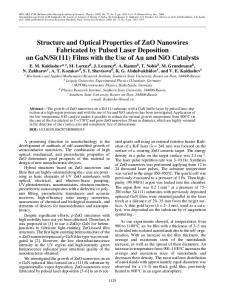
along the line segments A ---> L > M > r > A --> H > K > r in the Brillouin zone. The narrow lowest valence band near -20eV corresponds to an atomic-like oxygen 2s
state, the upper valence bands are mainly derived from the oxygen 2p state with a
sizable mixture of Zn 4s and 4p states. The lowest conduction band is composed
primarily of Zn 4s states. These bands reproduce those of Reference [18] quite accurately.
35
22.0
18.0
14.0
10.0
6.0
2.0
-2.0
-6.0
-10.0
-14.0
-18.0
-22.0
A
L
M
F
A WAVE VECTOR K
Figure 3.3 The Bulk band structure of the ZnO crystal.
H
K
F
36
Chapter 4
A Simple Model for Surface
The surface of dielectric materials is of major interest in our research. We investigate simple one-dimensional models in this chapter before we attack the real two-
dimensional surface. How the intrinsic atomic properties and the structures beneath the surface determine the surface behavior is easier to understand using these simple models
as a guideline. Also these simple models show some generic features of surfaces.
Furthermore, the discussion of these models tells us about the convergence properties of the calculations for our ZnO surface model.
4.1 The One-Dimensional Model Suppose that N objects are located in one-dimensional chain as shown in the following figure.
00 Although each object may have many single-object eigenstates, we assume that only one
particular eigenstate for each object is coupled to its nearest neighbor after an interaction
is turned on between the nearest neighbors. To simplify our description, we assume each object has only one eigenstate. We use $1); to denote the eigenfunction of the ith object. The energy spectrum of this chain is simply composed of single-object energy levels
before we turn on the interactions, and it consists of only one N-fold degenerate level if
all the objects are the same. The degeneracy will decrease and the spectrum will change
after the interactions are turned on. The coupled chain system has a new set of
37
eigenstates with eigenfunctions {4:13l
i = 1, ,N}. Each eigenfunction (V is a
superposition of the single-object eigenfunctions as in equation (4.1): sztoj =
1
ajA
(4.1)
2
where 'aft' indicates the weight of 4 in cl)j.
If the Hamiltonian of the coupled chain is
denoted as H, the Schrodinger equation is, HO] = Elcbj
j=1,,N
(4.2)
where E' is the energy of the eigenstate with eigenfunction In the space of {0i i = 1, -,N}, the Hamiltonian of the coupled one-dimensional chain system looks like the following tridiagonal matrix:
0
0
0
0
0
0 0
(4.3)
H =[kii=[(4) JIHIO ,)1= 0 0
0 0
0
0
x 0
x
x
x
x
In this Hamiltonian matrix of equation (4.3), only those elements marked x are possible nonzero elements. The dimensionality of this matrix is equal to the number of objects of
the chain N. By diagonalizing the Hamiltonian matrix (4.3) we obtain the energy spectrum
IE-11, with j = 1,- ,N N. At the same time, we obtain the coefficients fafil in equation (4.1) as the eigenfunction for the jth eigenstate. In the rest of this chapter, we will study several one-dimensional models.
38
4.2 Identical Objects in a Chain
4.2.1 Case one The simplest case of our one-dimensional model is when all the objects are the same.
First we ignore the boundary effects or the terminal effects. Hence, the diagonal
elements of the Hamiltonian matrix take the same values and we set them equal to zero. The nonzero off -diagonal elements represents the coupling strength between nearest
neighbors, and we assign the value of one to all of them since they are equal to each
other in this case. We studied this model with various values of N, and we draw the following three major conclusions: 1.
The distribution of the ordered eigenvalues is smooth. There are no sharp jumps.
2. The single-object eigenfunctions are mixed "evenly". There are no localized states. The mixing of the basis functions creates standing waves.
3. The upper and lower bounds of the energy spectrum will increase as we increase the number of objects on the chain. However, they will quickly reach certain limits ( see figure 4.1 ).
Figure 4.1 shows seven sets of spectra corresponding to seven different values of the
total number of objects in the chain. As we can see from this figure, the upper (lower) bound of the spectrum is equal to 1.00(-1.00) when N is 2, but the bound becomes very
close to the limit 2.0(-2.0) when N is 20. Figure 4.1 also shows spectra for N=40 and N=80, and the corresponding bounds are almost equal to the limit. Next, we study the effects of terminating the chain differently. We will vary the value of the first diagonal element of the Hamiltonian matrix or the coupling strength
between the first and the second object to study the surface effects.
39
ate,
2.0
A A A A A
0 O
*404
A
÷ +
o
0
0
****
*It*
* ** **
A
*
* * *
A
+
0
A
* *
A
1.0 ' 0
o
*
* *
A
*
A
0
*
*
A
*
A
0 +
N 00 ;11
* *
A
.
r)
* *
A
:
A
0.0 430
A
* * *
0
el)
c4
A
+
A
o
O
* *
*
* * * *
A
0
A
A
O
A
-2.0 Ni*** 0
**
*
** A ** 0 A ** A ** 0
0
**
A
O
-
* *
A
o
÷
N=5 + N=10 ° N=20 A N=40 N=80
*
A
-1.0 IC
. N=3
0-
A
N=2 0
* 4
A
+
*
*
A
20
40
60
State n
Figure 4.1 Energy spectra corresponding to different numbers (N) of objects in the 1D model.
80
40
4.2.2 Case two The environment of the terminal object is different from other objects on the
chain. As a result of this environmental difference, the first order correction to the eigenvalue of the terminal object is different from the first order corrections to the
eigenvalues of the other objects. That is:
"
As this shows, we do not make H
Hu for i = 2,- -,N different from others in this model in order to
simulate a semi - infinite chain. In this case we still assume that all Huti values are equal.
To be specific, we consider Hu # 0 and take ki= 0 for i = 2, ---,N N. After varying Hu
,
we found that: 1.
There is no localized end state if H11 is small comparing to the coupling strength ( or the off -diagonal elements ). There may exist a few states that have a larger
weight of the end object than others, but the eigenfunctions of these states do not decay exponentially from the end into the chain. The eigenvalues are still confined between the upper and lower limits when Hu is smaller than the value
of the coupling strength. See figure 4.2.
2. One localized end state will appear when Hu is larger than the value of the coupling strength. In this case, the eigenvalue of the localized end state is above the upper limit in the spectrum if H11 is positive (see figure 4.3); it is below the lower limit if H11 is negative. The eigenfunction of this end state decays
exponentially as it goes into the chain (see figure 4.4). The exponent is related to the gap that is defined as the difference between the eigenvalue of the end state
and the upper bound. See figure 4.5. Figure 4.2 shows the energy spectra corresponding to values of 0.25, 0.50, 0.75 and 1.00 respectively for H11. We can see that the spectrum is not significantly changed
41
2.0
ii"-H11 =0.25
0 H11=0.50
se *U
H11 =0.75
1.0
+ H11=1.0 a
il
11
*
4
I
-1.0 *
m mill
-2.0
oolismill
0
20
40
60
80
State n
Figure 4.2 Energy spectra of the 1D model with a small difference between the eigenvalues of the terminal object and the others.
42
4.0
H11=1.25 o H11=1.50 x H11=1.75
A
o
Hui 2.00 * H11=2.25 H11=2.50 * H11=2.75
2.0
H1=3.00
ase le seal'
a a
a a a
a a
a aa
ass
aa
0.0
a ae a aa
/as a
aaa a a
a*
-2.0
0
20
40
60
80
State n
Figure 4.3 Energy spectra of the 1D model with a large difference between the eigenvalues of the terminal object and the others.
43
1.0e+00
............... 1.0e-10
.-
We. 00 4141A.0xx 000
A
X. 0A x *A 0
. .4.,... In ..
-0°00_
. 141M
"0"0-
000
x
**AA% 0 A A0_
. 6.10.1-
. Ulkom.,
00 'Do-"0 ,, °00 op x. 000 0,0 II A A 0A x. 000 co, we have t.k > 0 and the summation approaches an integration. For the bulk calculation, E. space is three dimensional and we write 5c- (al:, , (0))
=_
v fd3ky, Fnn, (EV2) o(h 0) j
E'en)
(6.13)
where V is the volume of the ZnO crystal and the integral is over any primitive cell of
the three dimensional reciprocal space. For our layered model, the £ space is two dimensional and we write 5--,(:),,,(.). 2
A 2 i d2iiI F... (Of n(,c;) OW (270
En .)
(6.14)
where A is the area of one layer and the integral is over a primitive cell of the two
dimensional reciprocal space. If we assume that the layered model contains L layers,
81
then its volume is V = L c x A, where c is the height of a ZnO crystal unit cell. So, equation (6.14) can be written:
(" (m)
8
Xab
V (2702 Lc
F (EV2)800) E n)
d2E
(6.15)
nn.
In the rest of this thesis, we calculate the susceptibility per unit volume.
6.1.3 The matrix element V bnk,- n' k'The matrix element VbnEn'-i, in equation (6.11) is defined as ivb145
vbni,n1.
(6.16)
where I n) is a single-particle wavefunction with band index n and wave vector E. From equations (3.4) and (3.7), we write 1 n) as follows:
In) = y, czokg,o) a,o
=
,-1
cn
Idelk.(A+3°)1a,o(T- (T? + ita)))
(6.17)
-s1
where I a, o(r (R + cia ))) is the wavefunction of the atomic orbital, 1? runs over all the
lattice vectors in the direct Bravais lattice. The direct Bravais lattice is simple hexagonal for our bulk calculation and it is a triangular net for our layered model
calculation. N is the total number of unit cells in the bulk case while it is the total number of atoms in a single layer in the layered model case.
c:, is the admixture
coefficient and it is also a function of the wave vector E. The index a of can0 represents one of the four basis atoms in a unit cell for the bulk case, and for the layered model case it represents the atom in a specific layer. Substituting equation (6.17) into equation (6.16) we obtain
82
Vbdi
= L L c ca.. 1
I (la 1\ b a,ov-q?+ ))1V '°
2., e
a,0 a'
+3..)))
F
(6.18)
In our calculation, we make the on site approximation. That is to assume (a, o(F 41?- + c70))1VbIa' ,o' ( r(k -Fila.)))= (a, o(F)IVb la' ,o')Sad8
(6.19)
After substituting (6.19) in (6.18) and summing over a' , R, and Re, we obtain
=
n *
.
can,e(a,o(7-)1Vbia,o' (F))8-kle
(6.20)
The integral of (a, o(F)1Vb la, o' (F)) in equation (6.20) is nozero only if one of o and o'
is the s-orbital while the other is pb orbital; b can be x , y , and z . We use a program written by Dr. Jansen to obtain the wave functions of the atomic orbitals. Then, the integral of (a, o(F)1V1a, o' (F)) is performed for atom Zn and atom 0 and the results are:
(Zn,px(F)111Zn,s(F))= 1.04
(0,p,(7-)I a 10,s(0)= 1.001 Combining equation (6.20) with either equation (6.13) or equation (6.15), we can
calculate the imaginary parts of the first order susceptibility for the bulk and layered model respectively.
6.2 DOS, JDOS, and
of of ZnO Bulk
The imaginary part of the first order ZnO bulk susceptibility is given by equations (6.13), (6.11), and (6.20), 2 =(oh11
(0)) = 17.1d3II( nn.
enRe[VameN,',4(ho) Eb.)
21rinhe)
(6.21)
83
where n' runs over the unoccupied conduction bands and n runs over the occupied
valence bands. Here, we assume zero temperature. To facilitate the computation we use the symmetry in the x-y plane of ZnO to convert the integral in (6.21) to one over only an irreducible segment of the Brillouin zone(BZ).
We use the linear analytic tetrahedron method[21] to evaluate the integral 51(a)," (0))
=
fd3kI( e" IBZ
nri
2
2/mho)
Re[VLVb.P(h03 En.n)
(6.22)
where IBZ stands for an irreducible segment of the BZ. To illustrate the method, we explain how the density of states and joint density of states are calculated.
6.2.1 Density of states and joint density of states The density of states per unit volume gn(e) for band n is defined as: gn (c) = (21t)3 f dko(e
en
(0)
(6.23)
1
where en (E) is the band energy function and the integral is over a primitive cell in k space. Since E = En (FC) represents a surface S. (c), we convert the integral of equation
(6.23) to an integral of f
ds
(271) s:/(01Ven(k)1
where the integral is over a
(6.24)
space surface inside a primitive cell on which the band
energies are the same for every wave vector k .
c n(E)1 is the absolute value of the
band energy gradient. The key to doing the integral numerically is to break the surface Sn (c) into many small pieces, with each small piece treated as a plane approximately.
This is done by dividing the primitive cell into many tetrahedrons. The contributions Agn (c) from each tetrahedron are calculated and added to give g(c).
84
Each tetrahedron has four vertices. We calculate the en (E) values at these four vertices and we obtain en (E) values anywhere else inside the tetrahedron by
interpolating linearly using the values obtained at the vertices. We find that if a tetrahedron contains a piece of the e = en (ii) surface, it may be either a triangle or a quadrilateral.
We denote values of the en (E) at four vertices by el, 82, 83, 84 and assume that: Et
E2
£3
E4
Then, the contribution Agn(e) from the tetrahedron is as follows:
e4
-1- vfo
2 1
Agn(e) =
e