be a geometric boundary, a sinuous river, a fractal or "area-like" coastline ... At scales much smaller than that of the source entity, the problem becomes one of.
�
EMPIRICAL COMPARISON OF TWO LINE ENHANCEMENT METHODS
Keith C. Clarke, Richard Cippoletti, and Greg Olsen
Department of Geology and Geography
Hunter College--CUNY
695 Park Avenue
New York, NY 10021, USA
e-mail: kclarke@everest .hunter.cuny.edu
ABSTRACT
Considerable recent cartographic research has focussed upon the theory, methods, and cartometry associated with the generalization of line features on maps . The inverse of the generalization transformation, enhancement, has received comparatively little attention with a few notable exceptions which use fractal methods . This study implements Dutton's enhancement method and uses the equivalent theory but an alternative method (Fourier Analysis) to present a parallel, but more analytically flexible technique . While the Fourier method requires an initial equidistant resampling of the points along a string, the reduced number of control parameters, and the shape-related metadata evident in the Fourier transform make the method an attractive alternative to the Dutton technique, particularly when further resampling is used. Test data sets from Dutton's work and for the Long Island, New York coastline were used to demonstrate and empirically compare the two methods . INTRODUCTION Cartography has been called a "discipline in reduction," in that the mapping sciences deal exclusively with the case where display takes place at scales smaller than those at which the data are captured, stored, or analyzed. Illustration of this concept follows from the consideration of a line feature on a map.
ENHANCED LINE (Larger scale)
Line as Digital Cartographic Object
Line (Smaller Scale)
As an "entity" in the real world, a line has a considerable number of properties . A linear feature on a map may be a geometric boundary, a sinuous river, a fractal or "area-like" coastline with indeterminate length, or a curve with a given expected smoothness such as a contour or fold line . This line is then geocoded and transformed into a spatial object called a string, a list of coordinates in some coordinate system which taken sequentially represent the entity inside a computer. Common-sense (and cartographic theory) tell us that the entity can then be symbolized and displayed accurately only at scales less than or equal to that of the source information . If the source of a coastline was a 1 :12,000 air photo, for example, the line can be shown with confidence at a scale of 1 :24,000 or 1:100,000. At scales much smaller than that of the source entity, the problem becomes one of generalization . This problem is particularly well understood in cartography, and has been the subject of considerable research (McMaster and Shea, 1992 ; Buttenfield and McMaster, 1991) . While applications of 72
"cartographic license" are occasionally necessary, (e .g . the movement or displacement of features, elimination or joining of islands, etc.) line generalization has traditionally focussed on reducing the number of points required to represent a line, with the constraint that the points continue to lie on the line, or be one of the original set of points (Douglas and Peucker, 1973). Consider, however, the inverse transformation . Cartographic enhancement seeks to increase the number of points used to represent a string as a cartographic object. Enhancem ent can be thought of as the compliment to generalization (Clarke 1982) . The goal of enhancement is to add detail to generalized maps and restore them to their original state. This may be nearly impossible where no high resolution variance data are available, but nevertheless enhancement can make cartographic lines more visually appealing for display pur poses . By parallel with generalization, we can state that enhancement can also take two forms . First, enhancement can simply densify the number of points given the existing line . An example of this type of representation would be the conversion of a line to a grid data structure or to Freeman codes . Sampling a line with a set of points which are equidistant along the line, separated with a fine spacing would be a similar example. The number of locations increases, though the line remains the same. Minor generalization will sometimes occur when points on the line are separated by at least half the grid spacing . Critical in this type of enhancement, termed emphatic enhancement, is the use of the original source string as the source of information in the enhanced line. This can be thought of as having all new points lie on or very close to the original line . Alternatively, we can apply a model to the line, and allow the model to generate points which are not constrained to the geometry of the original line. This type of enhancement is synthetic enhancement, in that the character of the line is imposed by the model used to enhance the line. In computer graphics, it is commonplace to enhance a line by fitting Bezier curves, Bessel functions, or B-splines (Newman and Sproull, 1979). These are mathematical models of the variation expected between points along the line, and assume that "smoothness," or continuity of the second derivative of a line is important. These methods are recursive by segment, that is they are applied to one segment at a time in a pass along the length of the string . In cartography, this type of smoothing enhancement is commonplace in contouring systems, where a curved and regular smoothness is expected by the interpreter, whether or not it is a good model of the actual data. Only one major alternative to this method for line enhancement exists, the fractal line enhancement algorithm of button (1981) . This method is also recursive by segment. DUTTON'S FRACTAL ENHANCEMENT METHOD It appears that Dutton has been alone in developing a technique to enhance the appearance of line detail. Dut ton's algorithm is based on the two related properties of fractals, self similarity and fractional dimensionality. "Self similarity means that a portion of an object when isolated and enlarged exhibits the same characteristic complexity as the object as a whole ."(button 1981, p. 24) Fractional dimension means "the Euclidean dimen sion that normally characterizes a form (1 for lines, 2 for areas, 3 for volumes)" (button 1981, p. 24) . Dutton's algorithm simply selects the midpoint of two adjacent line segments and moves the vertex out at a specified angle (Buttenfield 1985) . Several parameters control the displacement of a vertex . The first is the Sinuosity Dimension (SD) . SD determines "the amount of waviness that the chains should possess after fractalization."(button 1981, p. 26) . The next parameter is the uniformity coefficient (UC). UC is the proportion of distance to displace each vertex toward the recomputed location . A UC of 1 is the maximum an angle can be moved . A UC of zero compensates for the effect of fractalization and the lines appear unaffected. UC can range to -1, though anything below zero moves the vertex in the opposite direction of the original angle's original position . The last two parameters are straightness (ST) and smoothness (SM) . ST is the maxi mum length at which a line segment will be altered . If a segment is greater than ST it will not be altered . This factor prevents the modification of long straight segments such as state and county boundaries. The last step is smoothing. Smoothing is used to enhanced the appearance of the lines for display purposes . In addition, smoothing can prevent the instances where line concavities result in generating a line which intersects itself. Dutton's algorithm was implemented by Armstrong and Hopkins when they altered the dig ital layout of a stream network through fractalizatine (Armstrong and Hopkins, 1983). The stream network is represented as a interconnecting chain of grid cell centroids, with each cell one square mile in size . When the chains were plotted several problems resulted due to the rectilinear nature of the data . The bulk of the prob lems were spikes and streams joining in grid cells further downstream. To solve these problems, the "chains were smoothed (using splines) before fractalizing."(Armstrong and Hopkins 1983) After initial smoothing, button's algorithm was applied and the chains were again smoothed . This resolved the problems and created a more natural appearance for the stream network. Dutton's fractal line enhancement technique was empirically tested and shown to provide convincing enhanced lines .
� � � � �
Dutton discounted the use of single rather than recursive mathematical transformations for enhancem ent . "Digitized map data resemble fractals much more than they resemble (continuous) functions which mathematicians normally study. Although certain cartographic objects, including both boundaries and terrain, can be approximated using real functions, e .g. trigonometric series, the difficulty remains of represent ing nonperiodic map features as well as ones that are not single-valued, i.e., places where curves reverse direc tion" (Dutton 1981, p. 25) . We have taken Dutton's statement as a challenge, and have implemented a Fourier Line Enhancement technique which is able to add detail to digital line data, and successfully deals with the problems which Dutton cites. FOURIER LINE ENHANCEMENT A new technique for line enhancement is presented here. The heritage of the method lies in image processing, shape analysis (Moellering and Rayner, 1979) and terrain analysis (Clarke, 1988, Pike, 1986). The mathematical model chosen to enhance the lines is that of Fourier analysis, which assumes that the two series of points (we treat x and y as independent series and conduct a separate one dimensional Fourier transform for each), can be abstracted as the sum of a set of periodic trigonometric functions . The method works as follows . First, the input string is resampled into two series (x and y) which are functions of a counter n, where n represents equidistant steps along the string, starting at the initial point (which is retained), and incrementing in equal distances along the line. This is similar to the so-called walking dividers method for computing the fractal dimension (Lam and DeCola, 1993) in that the line is resampled by uniform steps of a pair of dividers set to some spacing. The spacing distance was user defined, but in all cases was some ratio of the minimum observed segment length . Each of the two sets of independent coordinates is then subjected to a discrete Fourier transform. The discrete transform is necessary since the length of the series is unknown until computation. The Fourier transform assumes that the original series in x and y are a sample from a set of trigonometric functions over a finite harmonic range . The full series, unsampled, is given by a transformed set of coordinates (u, v), which can be computed at any interval over the length of the series. The computer code for the series is adapted from Davis (1973), and has been rewritten in C. The computer program computes for each series two floating point vectors of Fourier coefficients, spaced as spatial harmonics rather than distances.
ui
kmax
= E
k=1
(Ak cos
(
kmax Vi =
Ak cos (
2knx a.
2kny i
(
k=1
) +B k sin (
t)
+
2knx . `) )
2kny .
B k sin (
~) )
The contribution of the harmonic number k can be computed from : 2 2 2 S k = A k +B k x, x, x,
2
SY, k
= A2 + B2 Y, k Y, k
S2 S2y, k x, k pk (x, y) = kmax + kmax S2 S2 x,k y, k k=1 k=1 In brief, the x and y series are abstracted by a set of combined sine and cosine waves of different amplitudes, wavelengths and phase angles . These angles are computed for harmonics, where the fast harmonic is the mean
of the series, and the second through kmax are of wavelength X of length n/k. Thus the sixth harmonic has a wavelength of one sixth of the length of the series . The S values are similar to variances in least squares methods, and combine to give the proportion of total variance contributed by any given harmonic pair P . Typically, the bulk of the variance combines into a few harmonic pairs . Choosing these pairs only, zeroing out the remainder of the Fourier series, and then inverting the series (computing x and y from the given A and B's) is exactly equivalent to smoothing the series . Enhancement of the series is now possible in either of two ways . First, the series can be oversampled into a large number of equidistant points, and then harmonics meeting a predetermined level of significance can be chosen for the inverse transformation . This inversion yields the same number of points as the resampling, which can then again be resampled by n-point elimination to give the desired level of detail . Alternatively, the complete Fourier series can be modified by applying an arbitrary function to the series which increases the high frequency end of the spectrum. The inverse transform then produces an emphatic enhancement by introducing more high frequency into the line. This method has been implemented in a C program which modifies the computed Fourier coefficients according to the following formulae: A k =Ak (1+ n_1 ),k=2 � ,n Bk=Bk(1+ n- 1),k=2, . .n This enhancement successively modifies the Fourier coefficients by a scaling, increasing from zero at the first harmonic (the series mean), one at the second harmonic, to two at the highest frequency harmonic . Thus successively higher frequency harmonics are amplified, yet by sufficiently small amounts that the Gibbs phenomenon is avoided. Both of the above methods were implemented, as computer programs in the C programming language and using data structures and utility programs from Clarke (1990) . Results were computed (i) for the same lines which Dutton used in his work and (ii) for a detailed digital shoreline of Long Island, New York. RESULTS The results of the analysis of Dutton's original test line are summarized in Table 1 . Several different runs of the Fourier analysis were performed on the line . The line was first transformed into the spatial frequency domain with the tolerance set to 0.0001 (tot=0.0001) of the total variance contributed to the series by any given harmonic. Any harmonic with an S value less than the tolerance was set to zero . The line was resampled to the minimum segment length (s = 1) . The result of the resampling produced a line of 71 segments from a line of 12 segments, giving an emphatic enhancement of the original line . The mean segment length and standard deviation of the segment lengths were increased . When the sampling interval is shortened to 1/3 of the minimum segment length (s = 3), the standard deviation of the segment lengths increased, which may be an artifact of the Gibbs phenomenon (see Figure 1) . As the tolerance is increased, fewer harmonics are used in the inverse transform. Consequently, the standard deviations increase, however, the lines are not being enhanced, but rather they are generalized due to fewer high frequencies remaining in the series . This generalization is not constrained by the geometry of the original line . Due to the very shoat nature of the line (12 segments) some obvious boundary effects occur at the ends. These could be alleviated by extending the lines, by forcing the first couple of segments to conform to the source line, or by truncating the line before the ends . The highpass spatial frequency filter was applied to a line resampled by the minimum segment length with the tolerance set to zero. All frequencies were retained in the inverse transform. The result of the highpass filtering was no different from the transform using a tolerance of 0.0001 and an s of l . The standard deviations of the segment lengths, the minimum, maximum, and mean segment lengths remained the same to two decimal places, however, upon visual interpretation (see Figure 2), there is a slight increase in the high frequency variation of the line . The effect is minimal. The result is comparable to an emphatic enhancement . This may be a result of the particular frequency distribution of the power spectrum. More variation in the "wiggliness" of the line was expected . This effect is explored further with a larger data set from a digitized portion of the coast of Long Island.
Table 1 : Number
Enhancement
SeoSments
Minimum Segment Length
Maximum Segment Length
Mean Segment Length
Standard Deviation of Segment Length
Dutton: Original Line
12
62 .55
975 .19
38 .43
27 .94
Dutton: Fractalized D=1 .1
36
47 .01
272 .72
124.19
63 .71
Dutton : Fractalized D=1 .5
39
58 .52
304 .25
139 .40
69 .02
Dutton : D = 1 .1 Smoothed
37
44 .63
605 .69
183 .97
125 .38
Dutton : D = 1 .5 Smoothed
39
59 .08
605 .05
200 .77
109 .74
.0001 s = 1 Fourier tot--0
71
20 .53
107 .01
67 .81
31 .36
Fourier to1=0 .0001 s = 3
220
2 .12
295 .22
34 .90
45 .78
Fourier to1=0 .002 s = 1
71
7 .76
764.51
109 .15
125 .62
Fourier to1=0 .002 s = 3
220
1 .01
434.35
39 .58
59.52
Fourier to1=0 .003 s = 1
71
8 .59
749 .02
108 .47
124 .23
Fourier tol=0 .003 s = 3
220
1 .29
335 .01
38 .21
50 .96
Highpass to1=0 .0 s = 1
71
20 .53
107 .01
67 .81
31 .36
A section of a digitized map of Lang Island was used to test the efficacy of the highpass algorithm on a real data set. The highpass algorithm was run with the same parameters as with the Dutton test line (tot=0 .0, s=1) . When the inverse transform was performed, the number of points in the line was significantly increased, and the segments became shorter and more similar . However, aesthetically, there was no visual difference between the original generalized line and the highpass filtered line, except for a slight increase in the roundedness of acute angles. This may be a result of the scale used for display, but as a result, another highpass algorithm was tested. The second highpass algorithm was designed to increase the high frequency portion of the spectrum more than the first algorithm . The second algorithm divided the power spectrum in half. The low end was left unadjusted, but the magnitude of the high frequency portion of the spectrum was doubled . The result was a coastline that appeared very realistic (see Figure 3) . The coastline had undulations, which appeared to be the result of mass wasting and wave action . This is to be expected because wave action is a circular motion, and the Fourier analysis uses a sinusoidal wave form as its model. Table 2 :
Enhancement
Number S oofments
Long Island: Original Line
lftnimum Segment Length
Maximum Segment Length
Mean Segment Length
Standard Deeiation tof Length
96
107 .57
4272 .91
807 .97
626.50
LI Highpass tot=0 .0 s = 1
696
73 .53
127 .68
107 .51
1 .98
LI Highpass2 tot=0 .0 s = 1
696
12 .37
582 .87
143 .38
297 .35
Figure 1
�
Original
Dutton Fractalized D=1 .1 Dutton : D= 1 .1 Smoothed
Highpass
Dutton : Fractalized D=1 .5 Dutton : D = 1.5 Smoothed
Figure 2
Figure 3
DISCUSSION
Like many algorithms, the Fourier enhancement method is controlled by a set of parameters . In our tests, we have found that three factors control the effectiveness of the technique and the character of the resultant enhancement . These are (i) the original distance used as a sampling interval to resample the points with equidistant spacing (ii) the amount of variance a harmonic should account for before it is included in the inverse Fourier transform, and (iii) the means of modification of the high frequency harmonics in the Fourier domain.
The choice of a proportion of the minimum segment distance in the line was made after several experiments with other measures, and was influenced by the relationship between our chosen mathematical model and the sampling theorem. Oversampling ensures that the enhanced line resembles the original line . We do not recommend sampling at distances greater than the minimum segment length, since the result is Fourier based generalization. This may be fine for smooth lines such as contours, but would not be good far coastlines . In addition, the choice of sampling interval determines the number of points in the analysis, the number of harmonics in the Fourier domain, and the number of points in the reconstituted enhancement . The use of oversampling followed by simple n-point elimination is seen as the most effective combination should a maximum number of points be desired in the final enhancement. Further research could include choosing sampling intervals which allow use of the Fast Fourier Transform, which would considerably increase computation speed . The criterion for inclusion of a harmonic in the inverse Fourier transform was the amount of variance or "power" of the particular harmonic . Setting the inclusion tolerance to zero includes all of the harmonics, and in all test cases, reproduced the original line almost perfectly . This property of the Fourier transform is highly desirable, since the Fourier domain then contains the same amount of information as the spatial domain. Even complex lines are remarkably well represented by a limited set of harmonics, yet as the number of harmonics falls (the tolerance increases) the limitations of trigonometric series for modeling complex lines become more marked. Lines can self-overlap (not always seen as a problem for complex coastlines) which leads to topological discontinuities . In some cases, one or two harmonics make a large difference in the shape of the line . Leaving them out produces boundary effects and degenerate shapes for the lines (figure 1) . The means of modification of the series is another control variable . Tests showed that several modifications of the Fourier coefficients aimed at increasing amplitudes at the high frequency end of the spectrum produced satisfactory results. While the simple method tested for the Dutton data proved adequate, again further research on the effects of different modifications of the higher frequencies is called for. A method which produced different "flavors" of wiggliness at the highest frequencies under the control of a single variable would be most suitable for enhancement purposes. CONCLUSION We have successfully implemented and tested an alternative method for the synthetic enhancement of cartographic lines . The method has been empirically shown to give results comparable to those of Dutton's technique . Our method uses (i) an equidistant resampling of the source line to yield independent x and y series, (ii) a discrete Fourier transform of these two series, (iii) modification in the Fourier domain by either extraction of significant harmonics or deliberate amplification of the higher frequency harmonics and (iv) the equivalent inverse Fourier transform back into the spatial domain . Advantages of the method are that it is a single, rather than a piecewise recursive mathematical transformation ; that it is analytic, i.e. the Fourier domain data have spatial meaning in terms of line shape, character, and fractal dimension; that it produces highly compressed Fourier domain representations of lines which can be retransformed to any scale, enhanced or generalized; and that it is computationally fast, especially in the Fourier to spatial domain transformation. In addition, lines with recognizably different character, from smooth to jagged, can be produced by the same method, including line with sharp directional discontinuities . Cartographers have traditionally argued that enhancement, as the opposite of generalization, is undesirable since its accuracy is by definition unknown. Nevertheless, the history of manual and computer cartography is full of instances of the application of "cartographic license," or perhaps "digitizer's handshake," especially for linear features. Our method is objective and repeatable, and yields results which are esthetically what a map reader expects to see . Where enhanced linework is acceptable, the advantages of holding an intermediate scale database from which both higher resolution and smaller scale maps can be created quickly on demand by one method has some distinct advantages to the cartographic practitioner . As an analytical bridge between esthetics and mathematics, the method also has much to offer the analytical cartographer. ACKNOWLEDGEMENT The authors would like to thank Geoff Dutton, who generously provided his FORTRAN code for implementing the Dutton enhancement algorithm .
REFERENCES Armstrong, M . P, Hopkins, L. D. (1983) "Fractal Enhancem ent for Thematic Display of Topologically Stored Data", Proceedings, Auto-Carto Six, vol. II, pp.309-318 . Buttenfield, B . (1985) "Treatment of the Cartographic Line", Cartographica, vo1.22, no .2 pp . 1-26 Buttenfield, B . P and McMaster, R . B . (Eds .) (1991) Map Generalization : Making Rules for Knowledge Rep resentation, J. Wiley and Sons, New York, NY Clarke, K.C . (1982) "Geographic Enhancement of Choropleth Data", Ph. D . Dissertation, The University of Michigan, University Microfilms, Ann Arbor, Ml . Clarke, K . C. (1988) "Scale-based simulation of topographic relief', The American Cartographer, vol. 15, no. 2, pp . 173-181 . Clarke, K . C . (1990) Analytical and Computer Cartography, Prentice Hall, Englewood Cliffs, NJ. Davis, J . C . (1973) Statistics and Data Analysis in Geology, J . Wiley, New York. Douglas, D . H., and Peucker, T. H.(1973) "Algorithms for the Reduction of the Number of Points Required to Represent a Digitized Line or its Caricature", The Canadian Cartographer, vol . 10, no . 2, pp. 112 122 . Dutton, G .H . (1981) "Fractal Enhancement of Cartographic Line Detail", American Cartographer, V.8, N .l, pp. 23-40 . Lam, N. and DeCola, L. (Eds .) (1993) Fractals In Geography, Englewood Cliffs, NJ, Prentice Hall . McMaster, R . B . and K. S. Shea (1992) Generalization in Digital Cartography, Association of American Geographers Resource Publication Series, Washington, D .C. Moellering, H. and Rayner, J . N . (1979) "Measurement of shape in geography and cartography", Reports of the Numerical Cartography Laboratory, Ohio State University, NSF Report # SOC77-11318 . Newman, W. M. and Sproull, R . F. (1979) Principles of Interactive Computer Graphics, McGraw-Hill, New York 2nd. Ed. Pike, R . J. (1986) "Variance Spectra of Representative 1 :62,500 scale topographies: A terrestrial calibration for planetary roughness at 0.3 km to 7.0 km", Lunar and Planetary Science, XVII, pp. 668-669 .