Paper accepted for presentation at 2009 IEEE Bucharest Power Tech Conference, June 28th - July 2nd, Bucharest, Romania 1
Energy Loss Estimation in Distribution Networks for Planning Purposes J. Dickert, M. Hable, P. Schegner, Member, IEEE
Abstract--Because of increasing economical pressures on network operators, the losses in the subtransmission and distribution systems are becoming more and more important. It is usually not economical to exchange equipment for the sole purpose of reducing losses; however, it is an important criterion when deciding to implement changes in the network. The computation of the energy loss with a network simulation program is very laborious and the required data is usually not available. In the paper, an energy loss estimation method based on readily available data (i.e. peak power, average power, power loss at peak load) will be derived and implemented. For this purpose already developed approximation formulas will be reviewed for the use in current networks with today’s load characteristics. The estimation is used to obtain the energy loss for different networks as well as for the possible reduction of energy loss due to reconfiguration of existing networks. To compare and verify the results of the energy loss estimation, a computation of the losses with a network simulation program is implemented and a time period of one year is analyzed. Index Terms--energy loss, energy loss estimation, loss analysis, loss factor, load factor, network planning
I. INTRODUCTION
D
ifferent network configurations are taken into consideration during the planning process of distribution networks. The challenge in the process is to observe all standards and criteria. This comprises for example voltage limits, current carrying capability of the equipment and the correct settings for the relays. Important focus of the engineering process should also be on reliability goals and economic operation of the network with little energy losses. Therefore, it is necessary to evaluate the losses in terms of costs, but costs can only be linked to energy losses and not to power losses. The costs of the losses have to be weighed up against investments as well as operation costs. Consequently, knowledge about the magnitude of the energy loss is J. Dickert is with the Laboratory of Electrical Power Systems and High Voltage Engineering, Technische Universität Dresden, 01062 Dresden, Germany (e-mail:
[email protected]). M. Hable is with the Siemens AG, Erlangen, Germany (e-mail:
[email protected]). P. Schegner Laboratory of Electrical Power Systems and High Voltage Engineering, Technische Universität Dresden, 01062 Dresden, Germany (email:
[email protected]). He is Dean of the Faculty of Electrical Engineering and Information Technology.
978-1-4244-2235-7/09/$25.00 ©2009 IEEE
important for the over-all comparison of different network configurations and should not be neglected. There are different ways for the evaluation of energy loss, but regardless of the method used, it is difficult to determine the costs exactly. One reason is the diversity of the losses in an electrical system. They can be generally divided into technical losses and non-technical losses. Technical losses are caused by current and resistance (I²R), hysteresis, eddy currents and dielectric losses (corona). Non-technical losses are for example due to metering errors, unmetered company or customer use and billing cycle errors. The complexity of the causes of the losses presents the difficulty of calculating them. Therefore an estimation based on proper reasoning meets certainly the needs for the network planner. Non-technical losses are not considered since they cannot be modelled and the network planner does not have direct impact on their magnitude. The paper describes an energy loss estimation method for network planning based on readily available data. The results of the energy loss estimation are verified with the results of the computation with a network simulation program. II. DETERMINATION OF ENERGY LOSS The determination of energy loss of a network can be done in many ways. The methods distinguish each other in terms of complexity, data acquisition, accuracy and whether the period under review is in the past or future. A. Measurement of Energy Loss Determining energy loss is theoretically a simple task for existing networks, but it can only be applied to past periods. The sold energy has to be subtracted by the bought energy to obtain the energy loss. This includes all technical as well as non-technical losses. The difficulty remains in the data acquisition for a specific date. This method cannot be applied to network planning since only the past can be reviewed. B. Computation of Energy Loss with a Network Simulation Program The computation of the energy loss is done by dividing the time period under review (e.g. 1 year) into time segments (e.g. 15 minutes), obtaining the data for the loads for each time segment and computing the power loss for each time segment with a network computation program. The power loss is multiplied by the considered time segment and summed up, which yields the energy loss. The summation approaches the
2
integral of the power loss of the time period under review. For this computation many data are necessary and the collection of the data is very laborious, more often than not impossible. Very often generic data have to be applied since the actual data are not available. For such a simulation in a distribution network the load curves for all customers in low voltage networks and for all ring main units for medium voltage networks are needed. Usually this information is not available. In medium voltage networks typically only the load curve in the incoming transformer is measured. In the ring main units only the peak current is measured by non-return pointers. In low voltage networks very often there is no current measurement at all. Only technical losses are considered in the computation and the time period under review can be in the past or future. This method is used in this paper to verify the results of the developed loss estimation method. C. Energy Loss Estimation Method The energy loss estimation method is based on the approximation of the loss factor by the load factor. For the approximation only information about the peak power, average power and power loss at peak load is needed. After all, only one load flow calculation has to be performed for the load losses and one for the no-load losses. This makes it easy to estimate the energy loss caused by technical losses with available data and in a very short time. The time period under review can be in the past or future. The theory and its application to network planning will be explained in the following sections. III. LOSSES, LOSS FACTOR, LOAD FACTOR AND THEIR RELATION A. Definition of Technical Losses Technical losses are typically divided into load losses (e.g. copper losses) and no-load losses (e.g. iron losses). Load losses are a function of current and no-load losses are a function of voltage. Since the grids are run nearly at constant voltage, the noload losses are also nearly constant. They can be calculated with one load flow calculation under the assumption that all units are in normal operation and all loads are switched off. The no-load losses include hysteresis, eddy currents and dielectric losses as well as I²R losses due to no-load currents. In contrast, the load losses are not constant and vary according to the loading of the equipment. They consist of heat losses in the conductors caused by the load cur-rent. The main focus for the energy loss estimation method is on the load losses since their computation is very difficult and they are differing in a wide range depending on the load characteristic. B. Loss Factor The loss factor Fs is defined as the average load loss Pload loss to the load loss Pload loss(Smax) at peak load Smax occurring in that period T. The relationship between the load
loss and the load current is illustrated in figure 1. T
Fs =
∫ 0 Pload loss ⋅ d t
(1)
T ⋅ Pload loss ( Smax )
Peak load Smax is the instant when the point of delivery supplies the peak load to the net and not the peak load of each customer. Equation (1) can be rewritten considering current and resistance (I²R), which cause the load losses. This gives equation (2), where Iload is the load current during a specific time period T and Iload(Smax) the load current occurring in that period T at peak load Smax. The link to load losses is the resistance R. The transmitted power S is proportional to the load current Iload. This relationship is also used in equation (2) to link the loss factor to the transmitted power. T
T
∫ 0 R ⋅ Iload ⋅ dt
Fs =
2
=
∫0 S
2
⋅dt
(2) 2 2 T ⋅ Smax T ⋅ ⎛⎜ R ⋅ I load ( Pmax ) ⎞⎟ ⎝ ⎠ The loss factor is also known as equivalent hours loss factor and can be interpreted as amount of time to give the same losses at peak load as that produced by the actual variable load over the time period under review [1], [2]. The period under review for network planning is usually one year.
(
)
Pload loss = R ⋅ I 2
I
R U load
U
Z load Sload = U load ⋅ I
R
Z load
U load ≈ const. → U load ≠ f ( I ) 2 Pload loss ≈ R ⋅ I 2 ∼ R ⋅ Sload
Fig. 1. Single-line diagram to illustrate the relationship between load loss and magnitude of load
C. Load Factor The load factor Fd is the ratio of average load S to the peak load Smax during a specific period T. It is assumed that the power factor cos(ϕ) of the loads is constant. T
Fd =
∫0 S ⋅ d t
(3) T ⋅ Smax It can be seen that the definitions of load factor (eq. (3)) and loss factor (eq. (2)) are quite similar. However, there is also a relationship between the two factors which depends on the shape of the load curve. The estimation of this relationship is used for the energy loss estimation method.
3
D. Boundaries of the Relationship between Load Factor and Loss Factor The relationship of the two factors depends on the shape of the load curve. Two extremely theoretical load curves SA and SB described by equation (4) are shown in figure 2. for 0 ≤ t ≤ Fd ⋅ T ⎧S SA = ⎨ max for Fd ⋅ T < t ≤ T ⎩0 ⎧ Fd ⋅ Smax ⎪ SB = ⎨ Smax ⎪F ⋅ S ⎩ d max
for
0 ≤ t ≤ 0.5 ⋅ T − Δτ
for
0.5 ⋅ T − Δτ < t ≤ 0.5 ⋅ T + Δτ
(4)
for 0.5 ⋅ T + Δτ < t ≤ T Load curve SA has two extremes, peak load or no load. The load factor depends on the length of the time intervals. This represents start-stop operation. In contrast to that is the continuous load curve SB. Only for a very short time interval it reaches the peak load Smax. The time interval of peak load has the length of 2 ⋅Δτ (with Δτ