COMPARING THE PERFORMANCE OF DIFFERENT META-HEURISTICS FOR UNWEIGHTED PARALLEL MACHINE SCHEDULING M.O. Adamu1∗ & A. Adewumi2 1
Department of Mathematics University of Lagos, Nigeria.
[email protected]
2
School of Mathematics, Statistics & Computer Science University of Kwazulu-Natal, Durban, South Africa
[email protected] ABSTRACT
This article considers the due window scheduling problem to minimise the number of early and tardy jobs on identical parallel machines. This problem is known to be NP complete and thus finding an optimal solution is unlikely. Three meta-heuristics and their hybrids are proposed and extensive computational experiments are conducted. The purpose of this paper is to compare the performance of these meta-heuristics and their hybrids and to determine the best among them. Detailed comparative tests have also been conducted to analyse the different heuristics with the simulated annealing hybrid giving the best result. OPSOMMING Die minimering van vroeë en trae take op identiese parallelle masjien met behulp van die gepaste gleufskeduleringsprobleem word oorweeg. Die probleem is nie-deterministies polinomiese tyd volledig en die vind van ‘n optimale oplossing is dus onwaarskynlik. Drie meta-heuristieke en hul hibriede word voorgestel en uitgebreide berekeningseksperimente word uitgevoer. Die doel van hierdie artikel is om die vertoning van hierdie metaheuristieke en hul hibriede met mekaar te vergelyk om sodoende die beste te identifiseer. Gedetaileerde vergelykende toetse is ook uitgevoer om die verskillende heuristieke te ondersoek; daar is gevind dat die gesimuleerde uitgloei hibried die beste resultaat lewer.
∗
Corresponding author South African Journal of Industrial Engineering August 2015 Vol 26(2) pp 143-157
1
INTRODUCTION
Due to an increased emphasis on satisfying customers in service provision, due-date related objectives are becoming more important in scheduling. In this article, the objective of minimising the number of early and tardy jobs is considered – a situation where more jobs are completed within their due windows (due-dates). This objective is practical in realworld situations, in order to attain a better customer service rating. To the best of our knowledge, no other article has considered this type of problem. Therefore, the purpose of this study is to compare the performance of several meta-heuristics and to determine a good meta-heuristic to solve this problem. In the identical parallel machine problem, n jobs are to be processed on m machines, assuming the following facts: • • • • • •
A job is completed when processed by any of the machines; A machine can process only one job at a time; Once a job is being processed, it cannot be interrupted; All jobs are available from time zero; The weights (penalties) of the jobs are equal (unweighted); and All processed jobs are completed within their due windows.
During the past few decades, a considerable amount of work has been conducted on scheduling on multiple machines [1] and single machine [2] in order to minimize the number of tardy jobs. When jobs in a schedule have equal important, they are referred to as 'unweighted' jobs, whereas 'weighted' jobs are cases where jobs' contributions are not the same. Garey and Johnson [3] have shown the problem considered in this work is NPcomplete; they argue that finding an optimal solution appears unlikely. Using the three-field notation of Graham et al. [4], the unweighted problem considered in this paper can be represented as Pm| |∑(Uj + Vj), ), where P describes the shop (machine) environment for identical parallel machines, and m describes the number of machines. The space between the bars is for possible constraints on the jobs such as pre-emption, release time, setup, batching precedence, etc. This current work considers job scheduling case on parallel machine with no explicit constraint. The symbols Uj and Vj are binary (0 or 1) that indicates whether a job is scheduled early or tardy respectively, that is, 0 is used when the job is scheduled on time, and 1 is used if it is not. Scheduling to minimise the (weighted) number of tardy jobs has been considered by Ho and Chang [5], Süer et al. [6], Süer [7], Süer et al. [8], Van der Akker [9], Chen and Powell [10], Liu and Wu [11], and M’Hallah and Bulfin [12]. Sevaux and Thomin [13] addressed the NPhard problem to minimise the weighted number of late jobs with release time (P|rj|∑wjUj). They presented several approaches to the problem, including two MILP formulations for exact resolution, and various heuristics and meta-heuristics to solve large size instances. They compared their results with those of Baptiste et al. [14], who performed better on average. Baptiste et al. [14] used a constraint-based method to explore the solution space and give good results on small problems (n < 50). Dauzère-Pérès and Sevaux [15] determined conditions that must be satisfied by at least one optimal sequence for the problem of minimising the weighted number of late jobs on a single machine. Sevaux and Sörensen [16] proposed a variable neighbourhood search (VNS) algorithm in which a ‘tabu’ search algorithm was embedded as a local search operator. The approach was compared with an exact method by Baptiste et al. [14]. Li [17] addressed the P|agreeable due dates|∑Uj problem, where the due dates and release times were assumed to be in agreement. A heuristic algorithm was presented and a dynamic programming lower bounding procedure developed. Hiraishi et al. [18] addressed the non-pre-emptive scheduling of n jobs that are completed exactly at their due dates. They showed that this problem is polynomially solvable, even if positive set-up is allowed.
144
Sung and Vlach [19] showed that when the number of machines is fixed, the weighted problem considered by Hirashi et al. [18] is solvable in polynomial time (exponential in the number of machines), no matter whether the parallel machines are identical, uniform, or unrelated. However, when the number of machines is part of the input, the unrelated parallel machine case of the problem becomes strongly NP-hard. Lann and Mosheiov [20] provided a simple greedy O (n log n) algorithm to solve the problem of Hiraishi et al. [18], thus greatly improving the time complexity. Čepek and Sung [21] considered the same problem of Hiraishi et al. [18], where they corrected the greedy algorithm of Lann and Mosheiov [20], which they argued was wrong; Hiraishi et al. [18] presented a new quadratic time algorithm that solved the problem. The single-machine scheduling problem to minimize the total job tardiness was considered by Cheng et al. [22 ] using the ant colony optimization (ACO) meta-heuristic. [23] compared scheduling algorithms for flexible flow shop problems with unrelated parallel machines, setup times, and dual criteria. Janiak et al. [24] studied the problem of scheduling n jobs on m identical parallel machines, where for each job a distinct due window is given and the processing time in unit time to minimize the weighted number of early and tardy jobs. They gave an O(n5) complexity for solving the problem (Pm|pj = 1 |∑wj(Uj + Vj). They also considered a special case with agreeable earliness and tardiness weights where they gave on O(n3) complexity (Pm|pj = 1, rj, agreeable ET weights|∑wj(Uj + Vj)). Adamu and Abass [25] proposed four greedy heuristics for the Pm||∑wj (Uj + Vj) problem, and performed extensive computational experiments. Adamu and Adewumi [26] proposed some metaheuristics and their hybrids to solve the problem considered by Adamu and Abass [25]; they found them performing better. 2
PROBLEM FORMULATION
Let there be an independent set, N = {1,2, . . . , n} of jobs that are to be scheduled on m parallel identical machines that are immediately available from time zero, each having an interval rather than a point in time, which is called the due window of the job. The left end and the right end of the window are called the earliest due date (i.e., the instant at which a job becomes available for delivery) and the latest due date (i.e., the instant by which processing or delivery of a job must be completed) respectively. There is no penalty when a job is completed within the due window, but for earliness or tardiness, a penalty is incurred when a job is completed before the earliest due date or after the latest due date. Each job jє N has a processing time pj, earliest due date aj, and latest due date dj; it is assumed that there are no pre-emptions and only one job may be processed on a given machine at any given time. For any schedule S, let tij and Cij(S) = tij +pj represent the actual start time on a given machine and completion time of job j on machine i, respectively. Job j is said to be early if Cij(S) dj, and on-time if aj ≤ Cij(S) ≤ dj. For any job k(ij), where k(ij) stands for the jth processed job on machine i, the number of early and tardy jobs [11] can be calculated by
1 1 U k (ij) = in t s ig n[Ck (ij) ( S ) − p j ] + 2 2
(1)
where we define that
1, sign[C k ( ij ) ( S ) − p j ] = − 1,
if a j > C k (ij ) ( S ) or
C k (ij ) ( S ) > d j
a j ≤ C k (ij ) ( S ) ≤ d j
and that int is the operation for making an integer. Obviously,
1, U k (ij ) = 0,
if a j > C k (ij ) ( S ) or
C k (ij ) ( S ) > d j
a j ≤ C k (ij ) ( S ) ≤ d j 145
Therefore, the problem of scheduling to minimise the number of tardy jobs on identical parallel machines can be formulated as m
W =∑ i =1
n
∑ j =1
m
Min W =
i =1
j =1
n
∑ j =1
1 1 int sign[C k (ij ) ( S ) − p j ] + 2 2 m
n
∑ ∑U i =1
3
m
U k (ij ) = ∑
k ( ij )
= min ∑ i =1
n
∑ j =1
(2)
1 1 int sign[C k (ij ) ( S ) − p j ] + 2 2
(3)
HEURISTICS AND META-HEURISTICS
3.1 Greedy heuristic Adamu and Abass [25] proposed four greedy heuristics that attempt to provide near-optimal solutions to the parallel machine scheduling problem. In this paper, the fourth heuristic (DO2) is used. It entails sorting the jobs according to their latest due date (i.e., latest due time - processing time) and the ties broken by the highest inverse ratio of processing time (i.e., 1 / processing time). The results of these greedy heuristics are encouraging; however, whether using metaheuristics and their hybrids can achieve better results will be investigated further. Similar codes used in Adamu and Adewumi [26] will be used to solve the problem of minimising the number of early and tardy jobs on parallel machines. 3.2 Genetic algorithm Genetic algorithm (GA) is one of the best known meta-heuristics for solving optimisation problems [27,28,29]. The technique is loosely based on evolution in nature, and uses strategies such as survival of the fittest, genetic crossover, and mutation. It has proved very useful in handling many discrete optimisation problems [30-32]; hence the decision to test its performance on the current problem and to compare it with the performance of greedy heuristics. An overview of the GA implemented for the current problem is presented as follows: 1.
2.
Problem representation: Deciding on a suitable representation is one of the most important aspects of a GA. An integer string representation is adopted in this study. Each job is fixed to a gene in the chromosome; this implies that the chromosome has length n (where n is the number of jobs). Each position in the chromosome therefore represents a job. Each gene contains two integer numbers representing the number of the machine to which the job will be assigned, and an order, respectively. The order number is a value between 1 and n, representing the order in which jobs assigned to the same machine will be executed. Genetic operators are then applied to both the machine number and the order. Figure 1 presents a typical representation for a case of five jobs (n = 5) to be processed on three machines. In this case, Jobs 1 and 4 should both be processed on Machine 2, but with Job 4 having priority over Job 1. Job 1
Job 2
Job 3
Job 4
Job 5
2 (2)
3 (1)
1 (1)
2 (1)
1 (2)
Figure 1: A sample representation for GA 3.
146
Algorithm: The pseudo code of the GA implemented is presented on the next page:
Generate a population of randomly initialised individuals. iterations← 0 repeat fori = 1 →popSizedo Perform crosssover with probability crossoverRate. end for fori = 1 →popSizedo forj = 1 →numJobsdo Mutate machine with probability mutationRate. end for end for fori = 1 →popSizedo forj = 1 →numJobsdo Mutate order with probability mutationRate. end for end for Use selection to form a new population of individuals. iterations←iterations + 1 untiliterations ≥ numIterations Return the fitness of the best individual. 4.
5.
Fitness function: The fitness function calculates the total number of jobs that could not be assigned to any of the machines so that they would finish between the earliest due date and the latest due date. For each machine, jobs that are assigned to it are placed in a priority queue (based on their respective order). Each job is then removed from the queue and placed on the machine. If the job were to finish early it would be scheduled to begin later (at earliest due date - processing time) in order to avoid the earliness penalty. However, if the job were to finish past the end time, it would not be scheduled at all; instead the job would be added to the total penalty (fitness). Since the fitness calculates the penalty incurred, it then implies that the lower the fitness function, the better the performance of the algorithms or the result generated. Genetic operators: The choice of basic operators of selection, crossover, and mutation influences the behaviours of the GA [29]. In the current study, the operators are applied separately to the machine and the order number. For both, the tournament selection was used to select the two parents for crossover. For the machine, the 1point crossover and conventional mutation was adopted. The mutation operator chooses a random machine from 0 to m-1 inclusive, and also changes the machine number randomly. Since the order number (the order in which jobs are to be processed on a machine) is permutation-based, swap mutation for the execution order was used. This involves randomly selecting two jobs to be processed on the same machine, and swapping the order in which they were originally to be processed. However, since there were no guarantees that these operators would allow for the best performance, further experimentation with variations of these operators was performed. More details will be given in a later section. Detail and basic descriptions of these operators can be found in Goldberg [27] and Mitchell [29].
3.3 Particle swarm optimisation Particle swarm optimisation (PSO) is regarded as another efficient optimisation technique [33,34], hence its selection for the current parallel machine scheduling problem. It is a population-based technique derived from the flocking behaviour of birds, and relies on both the particle’s best position found so far and the entire population’s best position, in order to get out of local optimums to approach the global optimum. PSO is appropriate to use for parallel machine scheduling since not much is known about the solution landscape. A description of the PSO, as implemented for this study, is presented on the next page: 1.
Problem representation: The PSO algorithm requires that a representation of the solution (or encoding of the solution) is chosen. Each particle will be an instance of the chosen representation. A complication is that PSO works in the continuous space, 147
whereas the scheduling problem is a discrete problem. Thus a method is needed to convert from the continuous space to the discrete space. The representation is as follows: • •
•
2.
Each particle is represented by a pair of two digits. The first digit is a number in the range [0,m), where m represents the number of machines on which the particle is scheduled. Note that 0 is inclusive and m is exclusive in the range. The number is simply truncated to convert to the discrete space. Similarly, the second digit, also in the range [0,m) represents the order of scheduling of the particle relative to other particles on the same machine; a lower number indicates that the job will be scheduled before jobs with higher numbers.
Algorithm: Below is a basic pseudo code of the PSO that was used. fori = 1 →PopSize do Construct particle with randomly initialised machine number and order. end for repeat pbest← 231 fori = 1 →PopSizedo fitness←calcfitness(pop[i]) if fitness rand(0..1) then sol←solPrime end if end if end for temp← temp*beta until temp ≤ templ
3.
4.
4
Fitness function: Since the solution is represented in virtually the same manner as a chromosome in the GA and a particle in PSO, the fitness function is calculated in the same way. That is, jobs pertaining to a particular machine are placed in a priority queue before being assigned to the machine. Those that cannot be assigned contribute towards the penalty. Operators: Although SA does not really have operators (in the sense of a GA having genetic operators), the SA algorithm does have to select a neighbour. The particular neighbour selection strategy that is used updates only a single element of the solution. The element is given a new randomly-chosen machine and a new order (done by swapping with the order of another randomly chosen element). By allowing for a high level of randomness when selecting the neighbour, it is ensured that good exploration will be achieved and that a local best is not found too early. COMPUTATIONAL ANALYSIS AND RESULTS
4.1 Data generation The program was written in Java using Eclipse. It actually consists of a number of programs, each one implementing a different type of solution. The output of each of these programs gives the final fitness after the algorithm has been performed, and the time in milliseconds that the algorithm took to run. The heuristics were tested on problems generated with 100, 200, 300, and 400 jobs, similar to Adamu and Abass [25], Adamu and Adewumi [26], Ho and Chang [5], Baptiste et al. [14], and M’Hallah and Bulfin [12]. The number of machines was set at levels of 2, 5, 10, 15, and 20. For each job j, an integer processing time pj was randomly generated in the interval (1, 99). Two parameters, k1 and k2 (levels of traffic congestion ratio) were taken from the set {1, 5, 10, 20}. For the data to depend on the number of jobs n, the integer’s earliest due date (aj) was randomly generated in the interval (0, n / (m * k1)), and the integer’s latest due date (dj) was randomly generated in the interval (aj + pj, aj + pj+ (2 * n * p) / (m * k2)). For each combination of n, k1, and k2, ten instances were generated; i.e., for each value of n, 160 instances were generated for 8,000 problems of 50 replications. The meta149
heuristics were implemented on a Pentium Dual 1.86 GHz, 782 MHz, and 1.99 GB of RAM. The following meta-heuristics were analysed: GA, PSO, SA, GA Hybrid, PSO Hybrid, and SA Hybrid. 4.2 Improvements The use of genetic operators of crossover and mutation for both exploration and exploitation of solution space gives the GA a unique advantage over some other metaheuristics. In this work, the original GA that was tested used 1-point crossover, random mutation for machines, swap mutation for order, and tournament selection. Other combinations of operators were also tested to check which ones improved the performance of the algorithm. This initial experiment showed that roulette-wheel selection, uniform crossover, and insert mutation (for order) are better for the problem at hand. A user can choose any combination of these operators to use to run the algorithm. More information on the optimal combination of genetic operators will be mentioned in Section 4.4. 4.3 Greedy hybrids This work seeks to improve the performance of the underlying meta-heuristics (GA, PSO, and SA) by potentially hybridising them with some features of the greedy heuristic proposed by Adamu and Abass [25]. The key feature of the greedy heuristics in that work essentially lies in the order in which jobs were assigned to machines. So the mechanisms of ordering in DO2 [25] are incorporated in the meta-heuristics (GA, PSO, SA). To implement the hybrid in the three meta-heuristics, the order field was removed from Gene, Dimension, and Element respectively. Also, any code in Chromosome, Particle, and Solution, which dealt with the order (e.g., swap mutation in Chromosome), was removed. 4.4 Parameter settings For each solutions strategy, there are a number of different parameters that affect the performance of the algorithm, such as population size, mutation rate, initial temperature, etc. These parameters were determined experimentally by running the algorithms on a subset of all the testing data, in order to determine the optimal parameters. This involved experimenting with the full range of each parameter and recording and tabulating the results achieved. The combination of parameters that gave the best performance was selected as the optimal combination. After this initial experiment, the optimal parameters for the GA were found to be as follows: • • • • • •
A population size of 10. Random mutation (for machines) used at a rate of 0.01. Swap mutation (for order) used at a rate of 0.01. Uniform crossover at a rate of 0.5. Tournament selection with a k set at 40 per cent of the population size. The number of iterations of the algorithm was set at 2,000.
The best performance with a population size of 10 for this initial experience is likely due to the inherently parallel nature of the GA; hence lower population size might give better runtime and fitness for problems of this nature where time is a critical factor. Further to the above parameters, the GA hybrid achieved best results when hybridised with the DO2 greedy heuristic. The optimal parameters for PSO are: • • • • • 150
A population size of 50. A w (momentum value) of 0.3. A c1 of 2. A c2 of 2. The number of iterations of the algorithm was set at 2,000.
Further to the above parameters, the particle swarm optimisation hybrid achieved best results when hybridised with the DO2 greedy heuristic. The optimal parameters for SA are: • • •
An initial temperature of 25. A final temperature of 0.01. A geometrical decreasing factor (beta) of 0.999.
Further to the above parameters, the SA hybrid achieved best results when hybridised with the DO2 greedy heuristic. 5
DISCUSSION OF RESULTS
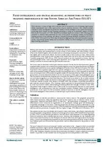
In this section, the results of the algorithms are shown, including the results of the hybridisations. In the four tables shown in Table 1 (a and b), each cell consists of two numbers. The top number is the weight of the schedule that is produced, averaged over 50 runs. The bottom number is the average time in milliseconds that the algorithm takes to complete. Also included are four charts, each for the performance of the meta-heuristics in relation to the penalty (see Figure 2) and time (see Figure 3) for n= 100, 200, 300, and 400. Figure 2 compares the relative performance (penalty) of each of the six algorithms with the number of machines used. Again, four charts are given to show the computational times of the meta-heuristics for various values of N. It should be clear from both Table 1 and the charts (Figures 2 and 3) that the SA Hybrid (SAH) outperformed the other meta-heuristics in almost all points. Its average performance time is 0.5 seconds. It was observed that the various hybrids performed better than their meta-heuristic without hybridisation. It further proves the effectiveness of hybridisation on the meta-heuristics. The GA performed worse than other meta-heuristics in all of the categories considered for all N jobs and M machines. The GA time is on the average less than two seconds, far slower than the SAH – notably because it keeps track of a population of individual solutions. Results show it to being in the region of four times slower than SAH. The GA that is hybridised with DO2 (GAH) achieves better results (see Table 1 and Figure 2) on all of the test cases than the simple GA. In all cases considered, the GAH outperforms the ordinary GA, and as the value of N increases, the performance rate of the GAH over the GA widens. For larger values of N, the performance of the GAH is almost equivalent to, if not better, than the SAH. The GAH takes on average about 2.55 seconds. The GAH would be ideal for larger values of N where an optimal solution is not readily feasible. It is observed that, on average, the GA takes less time to run than the GAH. The PSO and the hybrid PSO (PSOH) produce a lower number of early and tardy jobs than the GA. Furthermore, they are far slower than all the meta-heuristics considered (over 33.1 times slower for PSO and 22.9 for PSOH in relation to the SA). This is understandable since PSO is a population-based algorithm, so a lot of work is done at each step. Hybridising PSO with the DO2 greedy heuristic produces results that are better than PSO for all cases. The PSOH is also about 1.45 times faster than PSO. While it is observed for all other metaheuristics that, as the number of machines increases, their corresponding penalties reduce, the reverse is the case for PSO and PSOH. The results for SA are far better on average than those for GA, PSO, AND PSOH, in performance of both penalty and time (see Tables 1 and 2 and Figures 2 and 3). On average, SA takes 0.45 seconds to run. However, it is about 4.41, 5.72, 33.1, and 22.9 times 151
152
Table 1a: Performance of meta-heuristics for different values of N (100 and 200)
GA GAH PSO n=100 PSOH SA SAH
GA GAH PSO n=200 PSOH SA SAH
MIN 113 1937 63 2781 80 13734 65 10093 74 422 67 516
m=2 AVE 119.38 2006.86 76.04 2904.34 90.42 14069.74 74.96 10771.24 81.68 482.36 78.58 564.34
MAX 126 2122 85 3063 104 14453 85 11765 91 609 93 641
MIN 105 1891 59 2641 80 13359 68 9625 69 391 56 484
m=5 AVE 110.84 1961.52 69.52 2770.62 93.44 13795.38 82.88 10251.9 75.84 439.5 66.7 506.38
MAX 116 2266 59 2938 103 14250 90 11172 81 516 75 562
MIN 96 1828 52 2484 83 13406 64 9375 59 375 47 437
m=10 AVE 103.14 1909.34 64.02 2628.76 92.08 13703.4 85.5 9993.76 67.46 425.06 58.32 470.62
MAX 109 1985 76 2782 99 14141 95 10922 76 485 71 500
MIN 92 1890 51 2485 82 13468 74 9234 54 390 41 437
m=15 AVE 98.68 1928.72 59.96 61 90.54 14622.4 83.82 10029.34 62.06 435.64 53.54 468.14
MAX 106 2000 67 2750 95 20687 93 10687 69 516 61 515
MIN 88 1922 41 2531 80 14187 72 9531 47 406 35 453
m=20 AVE 93.26 1987.5 51.8 2648.48 88 15614.72 80.48 10251.54 54.36 459.08 46.28 476.62
MAX 101 2094 62 2813 95 18344 87 11109 64 531 57 532
MIN 105 1922 32 2797 57 14187 33 9953 49 421 32 531
m=2 AVE 112.74 2014.68 43 2889.16 69.68 15639.1 42.38 10685.86 57.2 470 44.12 553.74
MAX 119 2640 53 3031 82 17656 54 11672 66 532 52 610
MIN 94 1844 25 2625 54 13953 31 9500 36 406 24 468
m=5 AVE 100.46 1948.48 38.1 2751.26 71.4 15253.88 52.34 10410.12 50.02 436.52 35.96 500.9
MAX 111 2453 45 2938 87 16884 63 20562 58 485 49 547
MIN 78 1844 22 2484 65 13750 46 9359 31 375 18 437
m=10 AVE 89.28 1915.86 35.68 2591.58 73.6 15079.68 57.24 10099.74 43.64 424.3 31.92 464.44
MAX 96 2297 43 2719 83 16750 65 18812 51 500 42 515
MIN 75 1875 22 2454 62 13875 49 9343 31 390 17 437
m=15 AVE 82.8 1922.2 31.94 2579.58 72.36 15277.78 57.46 10094.66 38.02 434.74 26.88 466.26
MAX 92 1985 39 2734 81 17157 65 18422 45 500 34 437
MIN 72 1890 18 2484 62 14218 48 9484 24 406 15 453
m=20 AVE 77.14 1986.2 27.86 2606.54 72.02 15587.76 56.64 10341.26 33.68 457.3 23.02 479.92
MAX 85 2625 36 2766 79 17687 67 19719 41 547 34 547
GA GAH PSO n=300 PSOH SA SAH
GA GAH PSO n=400 PSOH SA SAH
MIN 96 1938 13 2765 44 14093 13 10125 32 422 14 516
m=2 AVE 109.28 2031.28 21.06 2868.62 57.7 15610.6 21 10898.8 42.26 479.12 21.6 551.54
MAX 127 3266 29 3047 69 18469 32 21672 56 563 32 609
MIN 85 1844 12 2609 42 13890 15 9610 28 391 13 468
MIN 94 1953 3 2766 42 14157 3 9921 23 422 3 515
m=2 AVE 106.38 2021.86 8.9 2861 54.72 15572.48 9.46 10640.96 43.2 468.78 9.32 549.7
MAX 118 2312 15 2938 66 17468 16 11672 42 532 16 609
MIN 81 1844 2 2640 37 13110 10 9437 18 406 1 468
m=5 AVE 94.9 1945.92 18.72 2745.68 57.38 15334.38 30.74 10250.84 34.84 448.86 18.04 501.16
MAX 105 2422 30 2938 75 17375 47 14594 44 547 29 578
MIN 71 1844 8 2500 50 13765 18 9266 19 375 7 437
m=10 AVE 82.52 1918.78 15.94 2579.72 63.2 15153.82 35.98 9850.64 28.36 432.72 13.86 459.1
MAX 95 2391 24 2656 72 17062 45 10750 36 516 21 500
MIN 67 1828 8 2500 41 13906 12 9094 18 390 4 437
m=15 AVE 74.3 1962.22 14.94 2561.46 61.44 15309.38 38.34 9849.82 24.88 435.64 11.96 461.88
MAX 83 2766 23 2687 70 17969 51 10610 35 485 19 500
MIN 60 1891 3 2485 56 14218 10 9078 13 406 2 437
m=20 AVE 68.26 2003.44 11.48 2592.92 61.96 15566.66 37.78 10079.08 20.1 451.26 8.4 463.8
MAX 76 2734 21 2688 72 18500 48 11203 29 516 16 516
m=5 AVE 93.22 1974.82 8.32 2716.32 52.88 14119.14 18.26 10122.72 25.88 442.44 8.22 496.56
MAX 107 3141 15 2782 71 16953 29 10922 33 500 16 532
MIN 63 1875 0 2500 36 12906 11 9297 14 375 0 437
m=10 AVE 79.1 1914.62 6.6 2566.86 56.24 13153.44 23.76 9868.22 20.28 417.8 5.74 460.06
MAX 93 169 18 2672 65 13516 37 10579 33 484 15 516
MIN 62 1844 0 2484 30 12953 12 9016 8 390 0 437
m=15 AVE 71.3 1974.86 4.84 2560.86 54.64 13333.5 27.26 9887.2 15.92 437.8 3.64 466.54
MAX 83 3016 12 2860 62 13641 39 11188 24 390 10 532
MIN 57 1938 0 2515 49 13265 1 9437 6 406 0 437
m=20 AVE 64.7 1993.8 3.16 2576.74 54.62 13559.38 25.84 10066.84 12.58 446.32 2 472.78
MAX 74 2625 13 2641 61 13906 40 13297 22 515 9 547
153
Table 1b: Performance of meta-heuristics for different values of N (300 and 400)
quicker than the GA, GAH, PSO, and PSOH, respectively. SA has the best overall time performance of all the meta-heuristics. Table 2: Homogeneous subsets PENALTY Scheffea Subset for alpha = 0.05 HEURISTICS
N
SAH
20
28.4050
GAH
20
30.5940
SA
20
41.6130
PSOH
20
47.1060
PSO
20
GA
20
Sig.
1
2
3
69.4160 91.5840 .147
1.000
1.000
Means for groups in homogeneous subsets are displayed. a.
Uses harmonic mean sample size = 20.000.
Chart for n = 100 140 120 100 80 60 40 20 0
Chart for n = 200 120 m=2 m=5
GA GAH PSO PSOH SA
100
m=2
80
m=5
60
m=10
40
m=10
m=15
20
m=15
m=20
0
m=20 GA GAH PSO PSOH SA
SAH
Chart for n = 300
Chart for n = 400
120
120
100
m=2
80
m=5
60
m=10
40 20 0 GA GAH PSO PSOH SA
SAH
100
m=2
80
m=5
60
m=10
40
m=15
20
m=20
0
m=15 m=20 GA GAH PSO PSOH SA
Figure 2: Meta-heuristics performance in relation to penalty 154
SAH
SAH
Chart for n = 100 18000 16000 14000 12000 10000 8000 6000 4000 2000 0
Chart for n = 200 m=2 m=5 m=10 m=15 m=20
18000 16000 14000 12000 10000 8000 6000 4000 2000 0
Chart for n = 300 18000 16000 14000 12000 10000 8000 6000 4000 2000 0
m=2 m=5 m=10 m=15 m=20
Chart for n = 400 m=2 m=5 m=10 m=15 m=20
18000 16000 14000 12000 10000 8000 6000 4000 2000 0
m=2 m=5 m=10 m=15 m=20
Figure 3: Performance time of the meta-heuristics Hybridising SA with the DO2 greedy heuristic (SAH) produces results that are slightly better than the SA solution for all cases considered. It produces the overall best results among the meta-heuristics in terms of performance in relation to penalty. The average timing is a little less than 0.5 seconds. Due to the equality of their variances, subsets of homogeneous groups are displayed in Table 2 using Scheffé’s method. The Scheffé test is designed to allow all possible linear combinations of group means to be tested. That is, pair-wise multiple comparisons are done to determine which means differ. Three groups are obtained: Group 1 - SAH, GAH, SA, and PSOH; Group 2 - PSO; and Group 3 – GA. These groups are arranged in decreasing order of their effectiveness. The worst among them is the GA. 6
CONCLUSION
We considered an identical machine problem with the objective of minimising the number of early and tardy jobs. The purpose of this study was to compare the performance of several meta-heuristics and determine a good meta-heuristics to solve this problem. Six meta-heuristics that incorporate a fast greedy heuristic were suggested because they gave promising results. Computational experiments and statistical analyses were performed to compare these algorithms. The SAH was the best among the various meta-heuristics. This research can be extended in several directions. First, these results could be compared with an optimal solution. Second, the environment with uniform or unrelated parallel machines could be a practical extension.
155
ACKNOWLEDGEMENTS The authors are grateful to the referee(s) for their useful comments that improved the quality of this paper. REFERENCES [1] [2] [3] [4] [5] [6] [7] [8] [9] [10] [11] [12] [13] [14] [15] [16] [17] [18] [19] [20] [21] [22] [23] [24]
156
Adamu, M.O. & Adewumi, A.O. 2015. Minimizing the weighted number of tardy jobs on multiple machines: A review. Asian Pacific Journal of Operations Research. In press. Adamu, M.O. & Adewumi, A.O. 2014. Single machine review to minimize weighted number of tardy jobs. Journal of Industrial and Management Optimization, 10(1), pp. 219–241. Garey, M.R. & Johnson, D.S. 1979. Computers and intractability: A guide to the theory of NP completeness. San Francisco: Freeman. Graham, R.L., Lawler, E.L., Lenstra, T.K. & RinnooyKan, A.H.G. 1979. Optimization and approximation in deterministic sequencing and scheduling: A survey. Annals of Discrete Mathematics, 5, pp. 287-326. Ho, J.C. & Chang Y.L. 1995. Minimizing the number of tardy jobs for m parallel machines. European Journal of Operational Research, 84, pp. 343-355. Süer, G.A., Baez, E. & Czajkiewicz, Z. 1993. Minimizing the number of tardy jobs in identical machine scheduling. Computers & Industrial Engineering, 25(1-4), pp. 243-246. Süer, G.A. 1997. Minimizing the number of tardy jobs in multi-period cell loading problems. Computers and Industrial Engineering, 33(3,4), pp. 721-724. Süer, G.A., Pico, F. & Santiago, A. 1997. Identical machine scheduling to minimize the number of tardy jobs when lost-splitting is allowed. Computers and Industrial Engineering, 33 (1,2), pp. 271-280. Van Den Akker, J.M., Hoogeveen, J.A. & Van De Velde, S.L. 1999. Parallel machine scheduling by column generation. Operations Research, 47(6), pp. 862-872. Chen, Z. & Powel, W.B. 1999. Solving parallel machine scheduling problems by column generation. INFORMS Journal on Computing, 11(1), pp. 78-94. Liu, M. & Wu, C. 2003. Scheduling algorithm based on evolutionary computing in identical parallel machine production line. Robotics and Computer Integrated Manufacturing, 19, pp. 401407. M’Hallah, R. & Bulfin, R.L. 2005. Minimizing the weighted number of tardy jobs on parallel processors. European Journal of Operational Research, 160, pp. 471-484. Sevaux, M. & Thomin, P. 2001. Heuristics and metaheuristics for a parallel machine scheduling problem: A computational evaluation. Proceedings of the 4th Metaheuristics International Conference, pp. 411-415. Baptiste, P., Jouglet, A., Pape, C.L. & Nuijten, W. 2000. A constraint based approach to minimize the weighted number of late jobs on parallel machines. Technical Report 2000/228, UMR, CNRS 6599, Heudiasyc, France. Dauzère-Pérès, S. & Sevaux, M. 1999. Using lagrangean relation to minimize the (weighted) number of late jobs on a single machine. National Contribution IFORS 1999, Beijing, P.R. of China (Technical Report 99/8 Ecole des Minesdes Nantes, France). Sevaux, M. & Sörensen, K. 2005. VNS/TS for a parallel machine scheduling problem. MEC-VNS: 18th Mini Euro Conference on VNS. Li., C.L. 1995. A heuristic for parallel machine scheduling with agreeable due dates to minimize the number of late jobs. Computers and Operations Research, 22(3), pp. 277-283. Hiraishi, K., Levner, E. & Vlach, M. 2002. Scheduling of parallel identical machines to maximize the weighted number of just-in-time jobs. Computers and Operations Research, 29, pp. 841-848. Sung, S.C. & Vlach, M. 2001. Just-in-time scheduling on parallel machines. The European Operational Research Conference, Rotterdam, Netherlands. Lann, A. & Mosheiov, G. 2003. A note on the maximum number of on-time jobs on parallel identical machines. Computers and Operations Research, 30, pp. 1745-1749. Čepek, O. & Sung, S.C. 2005. A quadratic time algorithm to maximize the number of just-in-time jobs on identical parallel machines. Computers and Operational Research, 32, pp. 3265-3271. Cheng, T., Lazarev, A. & Gafarov, E. 2009. A hybrid algorithm for the single-machine total tardiness problem. Computers & Operations Research, 36(2), pp. 308–315. Jungwattanakit, J., Reodecha, M., Chaovalitwongse, P. & Werner, F. 2009. A comparison of scheduling algorithms for flexible flow shop problems with unrelated parallel machines, setup times, and dual criteria. Computers & Operations Research, 36(2), pp. 358–378. Janiak, A., Janiak, W.A. & Januszkiewicz, R. 2009. Algorithms for parallel processor scheduling with distinct due windows and unit-time jobs. Bulletin of the Polish Academy of Sciences Technical Sciences, 57(3), pp. 209-215.
[25] Adamu, M. & Abass, O. 2010. Parallel machine scheduling to maximize the weighted number of just-in-time jobs. Journal of Applied Science and Technology, 15(1-2), pp. 27–34. [26] Adamu, M.O. & Adewumi, A.O. 2012. Metaheuristics for scheduling on parallel machines to minimize the weighted number of early and tardy jobs. International Journal of Physical Sciences, 7(10), pp. 1641-1652. [27] Goldberg, D.E. 1989. Genetic algorithms in search, optimization and machine learning. AddisonWesley. [28] Holland, J.H. 1975. Adaptation in natural and artificial systems. Ann Arbor, MI: University of Michigan Press. [29] Mitchell, M. 1998. An introduction to genetic algorithms. The MIT Press. [30] Adewumi, A.O. & Ali, M. 2010. A multi-level genetic algorithm for a multi-stage space allocation problem. Mathematical and Computer Modeling, 51(1-2), pp. 109-126. [31] Adewumi, A.O., Sawyerr, B.A. & Ali, M.M. 2009. A heuristic solution to the university timetabling problem. Engineering Computations, 26(8), pp. 972-984. [32] Naso, D., Surico, M., Turchiano, B. & Kaymak, U. 2007. Genetic algorithms for supply-chain scheduling: A case study in the distribution of ready-mixed concrete. European Journal of Operational Research, 177, pp. 2069–2099. [33] Arasomwan, A. M. & Adewumi, A. O.,2013. On the Performance of Linear Decreasing Inertia Weight Particle Swarm Optimization for Global Optimization, The Scientific World Journal, 2013, Article ID 860289, 12 pages. doi:10.1155/2013/860289. [34] Poli, R., Kennedy, J. & Blackwell, T. 2007. Particle swarm optimization: An overview. Swarm Intelligence, 1, pp. 33–57. [35] Kirkpatrick, S., Gellat, C. & Vecchi, M. 1983. Optimization by simulated annealing. Science, 220, pp. 671–680. [36] Chetty, S. & Adewumi, A.O., 2013. Three New Stochastic Local Search Metaheuristics for the Annual Crop Planning Problem Based on a New Irrigation Scheme. Journal of Applied Mathematics, 2013, Article ID 158538, 14 pages. http://dx.doi.org/10.1155/2013/158538.
157