entanglement production in a chaotic quantum dot

Fundamental Problems of Mesoscopic Physics Interactions and Decoherence

NATO Science Series A Series presenting the results of scientific meetings supported under the NATO Science Programme. The Series is published by IOS Press, Amsterdam, and Kluwer Academic Publishers in conjunction with the NATO Scientific Affairs Division Sub-Series I. Life and Behavioural Sciences II. Mathematics, Physics and Chemistry III. Computer and Systems Science IV. Earth and Environmental Sciences V. Science and Technology Policy

IOS Press Kluwer Academic Publishers IOS Press Kluwer Academic Publishers IOS Press

The NATO Science Series continues the series of books published formerly as the NATO ASI Series. The NATO Science Programme offers support for collaboration in civil science between scientists of countries of the Euro-Atlantic Partnership Council. The types of scientific meeting generally supported are “Advanced Study Institutes” and “Advanced Research Workshops”, although other types of meeting are supported from time to time. The NATO Science Series collects together the results of these meetings. The meetings are co-organized bij scientists from NATO countries and scientists from NATO’s Partner countries – countries of the CIS and Central and Eastern Europe. Advanced Study Institutes are high-level tutorial courses offering in-depth study of latest advances in a field. Advanced Research Workshops are expert meetings aimed at critical assessment of a field, and identification of directions for future action. As a consequence of the restructuring of the NATO Science Programme in 1999, the NATO Science Series has been re-organised and there are currently Five Sub-series as noted above. Please consult the following web sites for information on previous volumes published in the Series, as well as details of earlier Sub-series. http://www.nato.int/science http://www.wkap.nl http://www.iospress.nl http://www.wtv-books.de/nato-pco.htm

Series II: Mathematics, Physics and Chemistry – Vol. 154

Fundamental Problems of Mesoscopic Physics Interactions and Decoherence edited by

Igor V. Lerner University of Birmingham, Birmingham, United Kingdom

Boris L. Altshuler Princeton University and NEC Research Institute, Princeton, New Jersey, U.S.A. and

Yuval Gefen The Weizmann Institute of Science, Rehovot, Israel

KLUWER ACADEMIC PUBLISHERS NEW YORK, BOSTON, DORDRECHT, LONDON, MOSCOW

eBook ISBN: Print ISBN:

1-4020-2193-3 1-4020-2192-5

©2004 Springer Science + Business Media, Inc. Print ©2004 Kluwer Academic Publishers Dordrecht All rights reserved No part of this eBook may be reproduced or transmitted in any form or by any means, electronic, mechanical, recording, or otherwise, without written consent from the Publisher Created in the United States of America

Visit Springer's eBookstore at: and the Springer Global Website Online at:

http://www.ebooks.kluweronline.com http://www.springeronline.com

Contents

Preface

xi

Part I Decoherence and Dephasing 1 Electron Dephasing in Mesoscopic Metal Wires Norman O. Birge and F. Pierre 1 Introduction τφ in pure Au and Ag samples 2 3 Possible explanations for saturation of τφ 4 Aharonov-Bohm experiments in large Cu rings 5 Conclusions 2 Decoherence effects in the Josephson current of a Cooper pair shuttle Alessandro Romito and Rosario Fazio 1 Introduction 2 The model 3 Results 4 Cooper pair shuttle with SQUID loops 3 Dephasing in disordered metals with superconductive grains M. A. Skvortsov, A. I. Larkin, M. V. Feigel’man 1 Introduction 2 Description of the formalism 3 Dynamics of the phase 4 Phase transition 5 Cooperon self-energy 6 Dephasing time 7 Magnetoresistance 8 Discussion 4 Decoherence in Disordered Conductors at Low Temperatures: the effect of Soft Local Excitations Y. Imry, Z. Ovadyahu and A. Schiller 1 Introduction

v

3 3 5 7 10 13 17 17 18 20 29 33 33 36 37 38 40 42 44 45 49 50

vi

FUNDAMENTAL PROBLEMS OF MESOSCOPIC PHYSICS 2 3 4 5

The vanishing of the dephasing rate as T →0: theory Experimental results A tunnelling model for loosely bound heavy impurities Conclusions

5 Quantum precursor of shuttle instability D. Fedorets, L. Y. Gorelik, R. I. Shekhter and M. Jonson 1 Introduction 2 Theoretical model 3 Analysis and results 6 Dephasing and dynamic localization in quantum dots V.E.Kravtsov 1 Introduction 2 Weak dynamic localization 3 Role of electron interaction on dynamic localization in closed quantum dots. 4 Dynamic localization in an open quantum dot and the shape of the Coulomb blockade peak. 5 Summary 7 Mesoscopic Aharonov-Bohm oscillations in metallic rings T. Ludwig and A. D. Mirlin 1 Introduction 2 Low-temperature limit: fully coherent sample 3 Dephasing by electron-electron interaction 4 Summary 8 Influence Functional for Decoherence of Interacting Electrons in Disordered Conductors J. von Delft 1 Introduction 2 Main results of influence functional approach 3 Origin of the Pauli factor 4 Calculating τϕ ` a la GZ 5 Dyson equation and Cooperon self energy 6 Vertex contributions 7 Discussion and summary Appendix 1 Outline of derivation of influence functional 2 Cooperon self energy before disorder averaging 3 Thermal averaging

51 55 58 61 65 65 66 69 75 75 78 91 93 97 99 100 100 104 112 115 115 118 121 122 125 127 130 131 132 135 136

vii

Contents Part II

Entanglement and Qubits

9 Low-frequency noise as a source of dephasing of a qubit Y. M. Galperin, B. L. Altshuler and D. V. Shantsev 1 Introduction and model 2 Results for a single fluctuator 3 Summation over many fluctuators 4 Simulations 5 Comparison with the noise in the random frequency deviation 6 Applicability range of the model 7 Conclusions 10 Entanglement production in a chaotic quantum dot C.W.J. Beenakker, M. Kindermann, C.M. Marcus, A. Yacoby 1 Introduction 2 Relation between entanglement and transmission eigenvalues 3 Statistics of the concurrence 4 Relation between Bell parameter and concurrence 5 Relation between noise correlator and concurrence 6 Bell inequality without tunneling assumption 7 Conclusion 11 Creation and detection of mobile and non-local spin-entangled electrons P. Recher, D. S. Saraga and D. Loss 1 Sources of mobile spin-entangled electrons 2 Superconductor-based electron spin-entanglers 3 Triple dot entangler 4 Detection of spin-entanglement 5 Electron-holes entanglers without interaction 6 Summary 12 Berezinskii-Kosterlitz-Thouless transition in Josephson junction arrays L. Capriotti, A. Cuccoli and A. Fubini, V. Tognetti and R. Vaia 1 Introduction 2 The model 3 Numerical simulations 4 Results 5 The phase diagram 6 Summary Appendix: PIMC in the Fourier space for JJA

141 142 150 154 158 162 162 163 167 167 169 171 171 172 173 175 179 179 180 189 193 197 198 203 204 205 206 208 212 214 215

Part III Interactions in Normal and Superconducting Systems 13 219 Quantum coherent transport and superconductivity in carbon nanotubes M. Ferrier, A. Kasumov, R. Deblock, M. Kociak, S. Gueron, B. Reulet and H. Bouchiat 1 Introduction 219 2 Proximity induced superconductivity in carbon nanotubes as a probe of quantum transport 221 3 Intrinsic superconductivity in ropes of SWNT on normal contacts 226 4 Conclusion 235

viii

FUNDAMENTAL PROBLEMS OF MESOSCOPIC PHYSICS

14 Quantum Hall ferromagnets, cooperative transport anisotropy, and the random field Ising model J. T. Chalker, D. G. Polyakov, F. Evers, A. D. Mirlin, and P. Wölfle 1 Introduction 2 Domain formation and the random field Ising model 3 Transport anisotropy arising from domain formation 4 Transport along domain walls 5 Concluding remarks 15 Exotic proximity effects in superconductor/ferromagnet structure F.S.Bergeret, A.F. Volkov and K.B. Efetov 1 Introduction 2 The condensate function in a F/S/F sandwich 3 Josephson current in a F/S/F/S/F structure 4 Effect of spin-orbit interaction 5 Induced ferromagnetism in the superconductor 6 Summary 16 Transport in Luttinger Liquids T. Giamarchi, T. Nattermann and P. Le Doussal 1 Introduction 2 Model 3 Transport at intermediate temperatures 4 Creep 5 Variable range hopping 6 Open issues 17 Interaction effects on counting statistics and the transmission distribution M. Kindermann, Yuli V. Nazarov 18 Variable–range Hopping in One–dimensional Systems J. Prior, M. Ortuño and A. M. Somoza 1 Introduction 2 Model 3 Model with geometrical fluctuations only 4 Hopping matrix elements 5 Quantum model 6 Fluctuations 7 Summary and conclusions 19 On the Electron-Electron Interactions in Two Dimensions V. M. Pudalov, M. Gershenson and H. Kojima 1 Introduction 2 Renormalized spin susceptibility 3 Effective mass and g -factor 4 Summary

239 240 242 244 247 249 251 252 254 259 262 263 270 275 275 276 277 278 280 282 285

295 295 297 298 301 304 305 306 309 309 311 318 324

Contents 20 Correlations and spin in transport through quantum dots M. Sassetti, F. Cavaliere, A. Braggio and B. Kramer 1 Introduction 2 The model 3 The characteristic energy scales 4 Sequential transport 5 Results 6 Discussion and conclusion

ix 329 329 331 333 335 339 345

21 349 Interactions in high-mobility 2D electron and hole systems E. A. Galaktionov, A. K. Savchenko, S. S. Safonov, Y. Y. Proskuryakov, L. Li, M. Pepper, M. Y. Simmons, D. A. Ritchie, E. H. Linfield, and Z. D. Kvon 1 Introduction 349 2 Ballistic regime of electron-electron interaction 351 3 Interaction effects in a 2D hole gas in GaAs 353 4 Electron-electron interaction in the ballistic regime in a 2DEG in Si 361 5 Interaction effects in the ballistic regime in a 2DEG in GaAs. Longrange fluctuation potential. 362 364 6 Comparison of F0σ (rsψ) in different 2D systems 7 Conclusion 367 Index

371

This page intentionally left blank

Preface

The physics of mesoscopic devices came to existence in the mid-eighties when it became apparent that due to the onset of global phase coherence in systems of smaller dimensions, conventional approaches fail to describe submicron and nanoscale systems. Such systems with sizes intermediate between macro- and micro (i.e. single-atomic sizes) are now referred to as mesoscopic. Mesoscopic physics remains the focus of intense experimental and theoretical activity for more than 15 years. This diverse field is continually fuelled by rapid advances in materials and nanostructure technology, and in low temperature techniques. A wide variety of new devices extremely promising for major novel directions in technology, including carbon nanotubes, ballistic quantum dots, hybrid mesoscopic junctions made of different type of materials etc, came to existence during the last few years. This, in turn, demands a deep understanding of fundamental physical phenomena on mesoscopic scales. As a result, the forefront of fundamental research in condensed matter has been moved to the areas, where that the interplay of electron -electron correlations and quantum interference of phase-coherent electrons scattered by impurities and/or boundaries is the key to such an understanding. In spite of a substantial recent progress and significant achievements in the understanding of, e.g., physics of quantum dots, quantum wires and nanotubes, a set of extremely important fundamental issues still remains unresolved. One of the most intriguing problems at the heart of mesoscopics is that of dephasing and decoherence at low temperatures. Numerous recent experiments on dephasing in quantum dots and wires have added a new dramatic twist to this problem which had beforehand seemed to be well understood. On the face of it, these experimental results contradict to the most fundamental principles of quantum theory. Our belief is that the situation is not that dramatic and that these new results will be understood within the mainstream theory of disordered electronic systems, as the problem of decoherence in mesoscopics is clearly a part of a wider problem of the electron-electron interaction. A very interesting related direction in mesoscopic physics is investigating the possibility of using normal and superconducting nanodevices for the implementation of quantum entanglement and quantum manipulations in scalable

xi

xii


systems. Most of the currently proposed implementations of quantum computing devices use quantum optical systems, characterised by long decoherence times and controllable dynamics. However, their large-scale integration is highly problematic. Mesoscopic normal and superconducting systems, and even more so hybrid and magnetic systems look as very promising possible alternatives. In particular, the employment of spin-related physics appears to be promising. the possibility to control the electron spin degree of freedom, and the relatively long coherence time of this degree of freedom led to the emergence of a new field – spintronics. In general, disorder and/or chaos which are inherent for mesoscopic devices make experimental manifestation of the interactions much richer than in pure bulk systems. The understanding of decoherence as well as other effects of the interactions is crucial for developing future electronic, photonic and spintronic devices, including the element base for quantum computation. In this rapidly changing area, regular meetings of leading researchers in the field play a very important role. The present volume contains review articles written by the key speakers of a joint NATO advanced research workshop – EURESCO conference held in September 2003 in Granada, Spain. The talks have been concentrated on the topics described above, so that the volume is divided into three parts covering these topics. Acknowledgements. We are thankful to the NATO Scientific Affairs Division and EURESCO (European Research Conference Organisation of the European Science Foundation) for providing an excellent opportunity for bringing together leading researchers working in mesoscopic physics. We gratefully acknowledge an additional support by the US Army Research Laboratory - European Research Office. We thank all the officers of EURESCO who helped in the organisation of this meeting, especially Irene Mangion for her patient help at all the stages of preparing the meeting, and Anne Guehl for smooth, helpful and efficient running of all the organisational errands at the meeting venue in Granada. BORIS ALTSHULER, YUVAL GEFEN AND IGOR LERNER

I

DECOHERENCE AND DEPHASING


∗ !"#

τφ ! " " # " τφ (T ) T −2/3 T " $ τφ % # $ " & ' ſ " * * τφ +; % & τφ $ " # =

"

!"#!

{ I. V. Lerner et al. (eds.), Fundamental Problems of Mesoscopic Physics, 3–16. © 2004 Kluwer Academic Publishers. Printed in the Netherlands.

+

$%%& '() ($ (*(* +-*

" " " "" & ſ ſ | "| "

ſ ſ " # "

$ ^ ! " = " τφ " ' ƀ ſ }_~ "

" $ " ># $ }`~ " = " τφ " " ># * "

/ / 1

= τφ };~ τφ " " /0 τφ ; % * ſ " " ?@ }~ ] " τφ ; % # ſ" ! $ * " ! " * τφ (T ) & τφ " $ ;{ % ? % *@ || ? @ } {~ * ># * τφ 0.3K * > % }{~ TK τφ τφ *

_

/ / 1

τφ (ns)

10

1

0.1

TK

T (K)

1

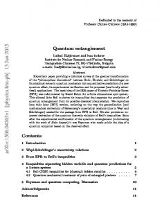
$2 300 ^ *?` @ ?•@ ^ *? @ ?◦@ *? @Mn0.3 ?@ *? @Mn1 ?@ " * ;{ " " *? @Mn0.3 *? @Mn1 " " %

TK = 40 % τφ ſ τφ (T ) = ? @ ƀ cmag " ſ ? τsf cmag = 1 @ ſ cmag = 0.13, ;{_ ;_` " *? @ *? @Mn0.3 *? @Mn1 " = }`~

" " > }`~ τφ " ?` @ * τφ *

" " ? ` @ τφ * ;{ ; > " " * ? ` $ @ * * " τφ " > τφ " 1K ſ τφ (T ) ƀ "

;

$%%& '() ($ (*(* +-*

> " =^ $ $ T > TK > ſ }`~ ſ ƀ " τφ > $ τφ ? = ƀ @ % " " }`~

,

-!/01-' *%#'! #! (& " #!&

% τφ ; τφ # " " }{_~ ^ τφ $"

" > kB T " ' " ƀ }+;~ τφ " " ? $ @ " τφ ſ ſ ƀ ?@ * ?*@ $ LT < Lφ LT = D/kB T & 1/2 1/4 Lφ ? τφ @ ſ 1/Lφ * $ " Lφ Lφ > * B ƀ τφ (B) ſ " ſ # /0 " " $ * " ſ " ?+; ; @

/ / 1

" ſ

' }+~ & = $" }~

δG (e2/h)

3

2

0.4

0.6

0.2

0.4

0.0

0.2

-0.2

0.0

-0.4 -0.05

-0.2 0.70

0.00 0.65

1

0

-0.8

-0.6

-0.4

-0.2

0.0

0.2

0.4

0.6

0.8

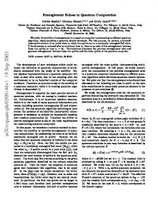
B (T) $2 30"0 > + e2 /h ſ T = 40 % * ?∆B 2.5 @ ƀ \ [ ' ſ * " ] [ ſ *

# * $ "

τφ ______ " ' " * τφ = * ƀ

$ ? = Lφ @ { ſ 1.5 µm T = 40 mK ?] T = 100 mK }~@ ſ " *

ſ

ſ ;; ; ;` ; & ſ * " " &

$%%& '() ($ (*(* +-*

* " " ≈ 2.4 mT 1.5 µm ] ſ * ? " @ ' ſ " $ ; ;{ ^ ;; % ſ ? + }~@ & * ſ ſ #@ }~ ' = * | " = = ſ e2 /h ? ; ] }++~@| *" " $ " " " # # }++~ ' LT = D/kB T # * " # = ; }+ +` ++~ $ LT < πr ? # * = " "

{

/ / 1

&5/ 3030 * $ [ ' LT Lφ ? $ @ ſ

D ?cm2 /s@

T ?%@

LT ?µm@

πr ?µm@

Lφ ?µm@

* *

}~ }+~ }+~

` ;;

+; ;

; { ;

+ { `

; ;_

LT < πr < Lφ πr < LT ≈ Lφ LT < Lφ < πr

LT " Lφ * LT < πr < Lφ Lφ < πr $ " = /0 * * * = * T −1 " LT ∝ T −1/2 Lφ

2

!("#!

= " $ τφ (T ) " ] ! & " * * τφ (T ) > 1 kF le @ " " * | | τφ = };~ = " ^ >]_;+ ;;+ " %= > " " ^ >]_;_` # = [ * * > * ^ X # ! " " & * \ * & = \& ' > * =

+! }~ / " \ * * \ ]* # X * ?__@ }~ * ^ "= $23 + ?_{@ $4 ?_+@ }{~ \ * * * / !/ " *\ > = X * ?_@ }+~ \ * * * % =" " 2 {` ?_@ }~ ^ # > ]

= = " ] \ 24 `{{ ?_`@ }`~ > > X> ' *\ " ] ,5 ` ?__{@ }~ > " > ]* # " ] \ 45 {{`` ?__@ }~ X ^ >X " ] \ 43 {+_; ?__@ }_~ * X \ " 5 ++ ?;;;@ };~ X >X \ " 5 +{ ?;;;@ }~ X >X * 6

1! / //

/ / 7

}~ }{~

}+~ }~ }`~ }~ }~ }_~ };~ }~ }~ }{~ }+~ }~ }`~ }~ }~ }_~ }{;~

}{~ }{~

" = X = * = % _ ?;;@ * " ?@ $6 + ?;;@ * * X >X /! * / 8 $ ! % ! " > > $ ^ ?;;@ ? ;;__@ * * X " ] \ 37 ;`;` ?;;@ " ] \ 53 ;`;+ ?;;@ * * * X " ] 65 ;+{ ?;;{@ > " ]* # " ] \ 3 ;```;+ ?;;{@ &\ * \ * > # ] > 3 ; ?___@ ^ * = " ] \ 5 ;+ ?__@ > * " ?\'@ 5 _ ?___@ ]> > ] ^ ^ ^ 3 ?__+@ > \ * ^ >" X $ > $ \ * > &\ * " ) ?__@ &" X =" ^ " \ ,4 `; ?___@ * = ] " ] \ 5) `{ ?___@ # * & X > > $2 ?_@ #* \ " 4 { ?_@ \ = \ " " = > ,7 {{ ?__@ &\ * \ * > " ] 6) ;+; ?;;@ ] ^' ^\ X X^ " ] \ )3 +; ?_@ \^ " &" /0 }+~ " * $ ^ &" " * ^ ? ;{{@ #X X " ] ,$ { ?__;@ &\ * '' " ] 66 ;+; ?;;@

`

$%%& '() ($ (*(* +-*

}{{~ \ * = " ] 65 ;++ ?;;{@ }{+~ ^ X= *& \= = " 6) ; ?_;@ }{~ " ] ] " ] ) {;_ ?_@ }{`~ \ " ] )) _ ?_`@ }{~ ^ # ] \ ^ " * ^ ^ " +{ " % ^ ?;;{@ ? ;{;``@ }{~ % # ] " X ^ * = ?_{@ }{_~ * " }+;~ * ' h/e * " = ' " " }+~ }+~ * ^ # ]* # >" \ /9 " * X =" ^ ?_@ }+~ > \& ' " ] 64 {; ?;;{@ }+{~ = X = " " ] )4 ; ?_@ }++~ ^ # ]* # ] " 22 { ?__@ }+~ ]* # ^ # ] \ ' " ] \ 2, `_` ?_@ }+`~ ^ # ] \ ' ]* # " ] )$ +_ ?_@ }+~ = > ]

= ^ # " ] \ 22 `; ?_@ }+~ X # /0 }+~ * * " Lφ ;

* }+_~ \ \ \ " \ 24 ?;;@ };~ τφ " \ "[ > , ]; ?;;@

Chapter 2 DECOHERENCE EFFECTS IN THE JOSEPHSON CURRENT OF A COOPER PAIR SHUTTLE Alessandro Romito and Rosario Fazio NEST-INFM & Scuola Normale Superiore, I-56126, Pisa Abstract

The effect of decoherence on the Josephson current between two superconductors when Cooper pair transport is achieved through the shuttle mechanism can be of great relevance. In this paper we analyze the DC Josephson current in several experimentally relevant situations. We show that decoherence effect, due to gate voltage fluctuations, can either suppress or enhance the critical current and also change its sign. The current noise spectrum displays a peak at Josephson energy and it is phase sensitive. We finally propose a device that has the shuttle properties but requires no mechanically moving part.

Keywords:

Cooper pair shuttle, decoherence, Josephson effect

1.

Introduction

The Josephson effect [1] consists in a dissipation-less current between two superconducting electrodes connected through a weak link [2, 3]. The origin of the effect stems from the macroscopic coherence of the superconducting condensate. Since its discovery in 1962, the research on devices based on the Josephson effect has been achieving a number of important breakthroughs both in pure [2] and applied physics [3]. One of the most recent exciting developments is probably the implementation of superconducting nano-circuits for quantum information processing [4], which requires the ability to coherently manipulate these devices. By now, this has been shown in several experiments in systems of small Josephson junctions [5–10]. Very recently, Gorelik et al. [11, 12] proposed a very appealing setup, the Cooper pair shuttle, able to create and maintain phase coherence between two distant superconductors. Shuttle systems have been subject of wide investigation in last years [13-15] (for a review see [16]). The Cooper pair shuttle [11, 12]

17 I. V. Lerner et al. (eds.), Fundamental Problems of Mesoscopic Physics, 17–31. © 2004 Kluwer Academic Publishers. Printed in the Netherlands.

18


consists in a superconducting SET transistor where the metallic grain is driven in a periodic motion between the two electrodes. The shuttling effect manifests in the fact that there is charge transport even though the grain, during is motion, is always in contact with only one of the electrodes. Following Gorelik et al. we also assume that both the grain and the electrodes are superconducting and that the charge transfer between the electrodes is coherent, namely due to Josephson effect. Despite the fact that the grain is in contact with only one lead at a time, the shuttle does not only carry charge, as in the normal metal case, but it also establishes phase coherence between the superconductors. This is witnessed by the presence of a steady state Josephson current. In this paper we analyze how the presence of the environment affects the coherent transport in the Cooper pair shuttle. As to the environment we consider the case in which it is determined by gate voltage fluctuations. Several interesting effects emerge. An increasing in the coupling to the environment may result in an enhancement of the supercurrent as well as in a change of its sign (π-junction). We propose an effective implementation of the shuttle mechanism. The paper, an extension of the results given in Ref. [17], is organized as follows. In section 2 we describe the system and the way we model it. In section 3 we describe in detail the way all calculations have been carried on. Subsections 3.1 and 3.2 are addressed to the presentation and discussion of results relative to DC Josephson current and current noise. In subsection 3.3 we discuss the current in the case of a particular choice of the applied gate voltage, which can be experimentally easier to realize. Finally, in section 4 we discuss a possible experimental realization of the shuttle mechanism by means of SQUID loops. The idea is that the same Hamiltonian of the Cooper pair shuttle can describe a system where the switching of the Josephson couplings is controlled by an external magnetic field. Such an implementation of the Cooper pair shuttle does not require any mechanical moving part.

2.

The model

The shuttle consists of a small superconducting island coupled to two macroscopic leads and forced to change its position periodically in time, with period T , from the Right (R) to the Left (L) electrode and back (see Fig.2.1). The grain is small enough so that charging effects are important, while the two leads are macroscopic and have definite phases φL,R . As long as the shuttle motion can be treated classically, the moving island is described by the Hamiltonian (b) n − ng (t)]2 − EJ (t) cos(φˆ − φb ) (2.1) H0 = EC (t)[ˆ b=L,R

where n ˆ is the number of excess Cooper pairs in the grain and ϕˆ is its conjugate phase, [ˆ n, ϕ] ˆ = −i. EC (t) = (2e)2 /2CΣ (t) is the charging energy, CΣ (t)

19

Decoherence in a Cooper pair shuttle (L,R)

being the total capacitance of the Cooper pair box. EJ (t) are the Josephson coupling to the left or right lead respectively, and ng (t) is the dimensionless gate charge. In fact the Hamiltonian (2.1) describes a more general system: a superconducting single electron transistor (SSET) in which Josephson energies and gate voltage vary in time, independent on the fact that this is a consequence of mechanical motion of the grain or not. As an interesting example we mention the recent proposal for a Cooper pair sluice where the Josephson couplings are varied adiabatically [18]. The Hamiltonian (2.1) corresponds to that of the shuttle if the time dependence of various parameters is given as described, for example, in Fig. 2.2. When the grain is close to one of the leads, the corresponding Josephson coupling is non-zero (with value EL , ER ) (positions L and R in (L) (R) Fig.2.1). In the intermediate region (position C), EJ (t) = EJ (t) = 0. As in Ref. [12] we employ a sudden approximation (which requires a switching time (L,R) ∆t 1/EL(R) ) and suppose EJ (t) to be step functions in each region (see Fig. 2.2). For late convenience we define the functions ΘL (t) = θ(t)θ(tL − t) (b) and ΘR (t) = θ(t−(tL +t→ ))θ(tL +t→ +tR −t), so that we can write EJ (t) = Eb n∈N Θb (t − nT ). The system operates in the Coulomb blockade regime, EJ max0From an experimental point of view, it would be easier to avoid the periodical modification of the gate voltage Vg to obtain ng (t) = 1/2 during the Josephson contacts. It can be therefore interesting to have an expression for the DC Josephson current in the case of constant gate voltage. If ng (t) = const. = 1/2, the Josephson current can be obtained from the expressions of section 3 with the replacement χ→ = χ← = 0. If ng (t) = const. = 1/2, instead, the general expression for for the current (Eq. (2.13)) still holds, but differences arise in the explicit form of matrix M0 and vector v0 . During the free evolution time intervals the dynamics is unchanged compared to the case discussed before. In the L and R regions instead, we have to include in the Hamiltonian the term proportional to the charging energy difference, EC , between the two charge states. In so doing, the whole Hamiltonian (system and bath), in the basis diagonalizing the Cooper pair box Hamiltonian, is H=

E ˆ σz + O(cos(2µ)σ z + sin(2µ)σx ) + Hbath , 2

(2.22)

where E = (EC2 +EJ2 )1/2 and cos(2µ) = EC / . The Hamiltonian in Eq. (2.22) has been widely studied [19]. In Born-Markov and Rotating Waves approximations the time evolution of populations (diagonal terms) in the reduced density matrix and coherences (off-diagonal ones) are still independent. The respective decoherence rates read pop.

γJ

= 2γJ sin2 (2µ) ,

γJcoher. = γJ sin2 (2µ) + ΓJ cos(2µ) .

(2.23) (2.24)

28


We notice that we have to introduce two different dephasing rates, γJ and ΓJ . In our approximation, they are γJ = (π/2)αE coth(E/Tb ), and ΓJ = 2παTb , in case of weak coupling of the system to the bath (α 1). Depending on the relative strength of the two energy scales EC and EJ , we have different effects. If EC = 0, (corresponding to 2µ = π/2) we recover the Hamiltonian of the early case described in section 3. If EC EJ , we have corrections of order EC /EJ in our previous results, and we are not interested in them as we get a finite result at zero order in EC /EJ . In the opposite limit EJ EC , the situation is quite different. Completely neglecting EJ , one obtains a null current because n ˆ is now a constant of motion. The first non vanishing term must be of order EJ /EC , and that is what we are interested in. We present the analytical expression for the current in the limit of strong dephasing (for tL = tR = tJ and t→ = t← = tC ). In such expression we include only the leading order in EJ /EC . The strong dephasing limit refers to the condition γJ tJ , ΓJ tJ , γC tC 1, which allows a series expansion of the Josephson current at first order in e−γJ tJ , e−ΓJ tJ and e−γC tC : 2e EJ 2 EC sin φ e−γC tC × Istrong ∼ − tanh T Tb EC coher. pop. coher. × sin(2χ) cos(2θ)e−γ tJ − e−γ tJ + cos(2χ)e−γ tJ . (2.25) In this cases the Josephson energy does not any more enter the current through the combination EJ tJ as in the previous case, but rather it appears through the ratio EJ /EC . There is an overall suppression factor ∝ (EJ /EC )2 . Note that the dependence on the dynamical phase χ, thou being obviously oscillatory, is not the same of that in Eq. (2.16). The approximation EJ EC also induces a hierarchy in the dephasing rates; γJcoher.

pop. γJ

∼2

EJ EC

2 γJ .

(2.26)

Within such approximation, we can neglect terms of order e−ΓJ tJ with respect coher. pop. to 1 (or equivalently e−γ tJ with respect to e−γ tJ ) in the current expression, leading to

Istrong ∼ −

2e tanh T

EC Tb

EJ EC

2

2 E − 2 EJ γJ tJ +γC tC

e

C

sin(2χ) sin φ .

(2.27) The exponential suppression due to dephasing in the Josephson contact times is reduced by the factor sin(2µ) ∼ (EJ /EC )2 .

Decoherence in a Cooper pair shuttle

4.

29

Cooper pair shuttle with SQUID loops

We conclude by suggesting a possible experimental test of our results which does not require any mechanically moving part. The time dependence of the Josephson couplings and ng is regulated by a time dependent magnetic field and gate voltage, respectively. The setup consists of a superconducting nanocircuit in a uniform magnetic field as sketched in Fig.2.6. By substituting the Josephson junction by SQUID loops, it is possible to control the EJ by tuning the applied magnetic field piercing the loop. The presence of three type of loops with different area, AL , AR , AC allows to achieve independently the three cases, where one of the two EJ ’s is zero (regions L,R) or both of them are zero (region C), by means of a uniform magnetic field. If the applied field is such that a half-flux quantum pierces the areas AL ,AR or AC , the Josephson couplings will be those of regions R,L and C, respectively and the Hamiltonian of the system can be exactly mapped onto that of Eq.(2.1). Moreover, by choosing the ratios AC /AR = 0.146, and AC /AL = 0.292 the two Josephson coupling are equal, (L) (R) EJ = EJ . This implementation has several advantages. It allows to control the coupling with the environment by simply varying the time dependence of the applied magnetic field. The time scale for the variation of the magnetic field should be controlled at the same level as it is done in the implementation of Josephson nano-circuits for quantum computation (see Ref. [4] for an extensive discussion). For a quantitative comparison with the results described here, the magnetic field should vary on a time scale shorter than /EJ , typically a few nanoseconds with the parameters of Ref. [5]. This is possible with present day technology [30]. At a qualitative level the results presented in this paper (π-junction behavior, non-monotonous behavior in the damping) do not rely on the step-change approximation of the Josephson couplings (which leads to Eq.(2.10)). Those effects are observable even if the magnetic field changes on time-scales comparable or slower than EJ . The only strict requirement is that only one Josephson coupling at the time is switched on.

Acknowledgments Part of the results presented here were obtained in collaboration with F. Plastina. We gratefully acknowledge many helpful discussions with G. Falci, Yu. Galperin and Yu.V. Nazarov. This work was supported by the EU (IST-SQUBIT, HPRN-CT-2002-00144) and by Fondazione Silvio Tronchetti Provera.

References [1] B. D. Josephson, Phys. Lett. 1, 251 (1962). [2] M. Tinkham, Introduction to Superconductivity, (McGraw-Hill, New York, 1996).

30


AC

AC AL

B(t)

AR

AC

AC

Figure 2.6. left: Sketch of the implementation of the shuttle process by means of a timedependent magnetic field. Crosses represent Josephson junctions. right: Plot of the time variation of the applied field (in unity of B0 = Φ0 /(2AC ),Φ0 is the flux quantum) in order to realize the (L) (R) Cooper pair shuttle. The different loop areas can be chosen in order to obtain EJ = EJ .

[3] A. Barone and G. Paternò, Physics and Applications of the Josephson Effect, (J. Wiley, New York, 1982). [4] Y. Makhlin, G. Schön and A. Shnirman, Rev. Mod. Phys. 73, 357 (2001) and references therein. [5] Y. Nakamura, Yu. A. Pashkin, and J. S. Tsai, Nature 398, 786 (1999); [6] J. R. Friedman, V. Patel, W, Chen, S. K. Tolpygo, and J. E. Lukens, ibid. 406, 43 (2000); [7] C. H. van der Wal, A. C. J. ter Haar, F. K. Wilhelm, R. N. Schouten, C. Harmans, T. P. Orlando, S. Lloyd, and J. E. Mooij, Science 290, 773 (2000); [8] D. Vion, A. Aassime, A, Cottet, P. Joyez, H. Pothier, C. Urbina, D. Esteve, and M. H. Devoret, ibid. 296, 886 (2002); [9] Y. Yu, S.Y. Han, X. Chu, S. I. Chu, and Z. Wang, ibid. 296, 889 (2002); [10] J. M. Martinis, S, Nam, J. Aumentado, and C. Urbina, Phys. Rev. Lett. 89, 117901 (2002). [11] L. Y. Gorelik, A. Isacsson, Y. M. Galperin, R. I. Shekhter, and M. Jonson, Nature 411, 454 (2001). [12] A. Isacsson, L. Y. Gorelik, R. I. Shekhter, Y. M. Galperin, and M. Jonson, Phys. Rev. Lett. 89, 277002 (2002). [13] L. Y. Gorelik, A. Isacsson, M. V. Voinova, B. Kasemo, R. I. Shekhter, and M. Jonson, Phys. Rev. Lett. 80, 4526 (1998). [14] A. Erbe, C. Weiss, W. Zwerger, and R. H. Blick, Phys. Rev. Lett. 87, 096106 (2001).

Decoherence in a Cooper pair shuttle

31

[15] D. L. Klein, R. Roth, A. K. L. Lim, A. P. Alivisatos, and P. L. McEuen, Nature 389, 699 (1997). [16] R. I. Shekhter, Yu. Galperin, L. Y. Gorelik, A. Isacsson and M. Jonson, J. Phys.: Condens. Matter 15, R441 (2003) [17] A. Romito, F. Plastina and R. Fazio, Phys. Rev. B 68, R140502 (2003). [18] A. O. Niskanen, J. P. Pekola, and H. Seppa Phys. Rev. Lett. 91, 177003 (2003). [19] U. Weiss, Quantum Dissipative Systems, (World Scientific, Singapore, 1999). [20] E. Paladino, L. Faoro, G. Falci, and R. Fazio, Phys. Rev. Lett. 88, 228304 (2002). [21] A. Romito and Yu. V. Nazarov, in preparation. [22] A. V. Shytov, D. A. Ivanov, M. V. Feigel’man, cond-mat/0110490. [23] The equation for time interval R is exactly the same ones the substitution L → R has been performed. [24] C. Cohen-Tannoudji, J. Dupont-Roc, and G. Grynberg, Atom-Photon Interactions, Wiley, New York (1992). [25] G. M. Palma, K.-A. Suominen, A. K. Ekert, Proc. Roy. Soc. Lond. A 452, 567 (1996). [26] J. H. Reina, L. Quiroga and N. F. Johnson, Phys. Rev., A 65, 032326 (2002). [27] The left-right and forward-backward symmetric case is defined by θL = θR = θ, γL tL = γR tR = γJ tJ and χ→ = χ← = χ, γ→ t→ = γ← t← = γC tC . [28] D. F. Walls and G. J. Milburn, Quantum Optics, Springer, Berlin Heidelberg (1994). [29] The general expression for the spectrum exhibits a divergence also in the limit (γJ , θ) → (0, kπ/2) due to the increasingly longer correlation time of the current fluctuations (see section 3). [30] O. Buisson, F. Balestro, J. Pekola, F. W. J. Hekking, to be publish in Phys. Rev. Lett.; F. Balestro, PhD thesis Universitè Joseph Fourier, Grenoble (unpublished).


Chapter 3 DEPHASING IN DISORDERED METALS WITH SUPERCONDUCTIVE GRAINS M. A. Skvortsov L. D. Landau Institute for Theoretical Physics, Moscow 119334, Russia

A. I. Larkin L. D. Landau Institute for Theoretical Physics, Moscow 119334, Russia Department of Physics, University of Minnesota, Minneapolis, MN 55455, USA

M. V. Feigel’man L. D. Landau Institute for Theoretical Physics, Moscow 119334, Russia

Abstract

Temperature dependence of electron dephasing time τϕ (T ) is calculated for a disordered metal with small concentration of superconductive grains. Above the macroscopic superconducting transition line, when electrons in the metal are normal, Andreev reflection from the grains leads to a nearly temperatureindependent contribution to the dephasing rate. In a broad temperature range τϕ−1 (T ) strongly exceeds the prediction of the classical theory of dephasing in normal disordered conductors, whereas magnetoresistance is dominated (in two dimensions) by the Maki-Tompson correction and is positive.

Keywords:

dephasing, superconductive fluctuations

1.

Introduction

During last few years, a number of experimental data on electron transport in disordered metal films and wires were shown to be in disagreement with the standard theory [1] of electron dephasing in normal conductors. Namely, at sufficiently low temperatures T ≤ T1 the dephasing rate τϕ−1 (T ) was system-


34


atically found to deviate from the power-law dependence [1]: ∼ (T /)3/2 τ 1/2 /(kF l)2 , 3D case, 1 = (0) τϕ (T ) (T /2πg) ln(πg), 2D case,

(3.1)

with a tendency to apparent saturation in the T → 0 limit (g = /e2 R 1 is dimensionless conductance of the film). Since no dephasing rate may exist at strictly zero temperature [2], such a behavior indicates a presence of some additional temperature scale(s) T0 (which may occur to be extremely low), so that in the range T0 ≤ T ≤ T1 the main contribution to τϕ−1 (T ) comes from some new mechanism, different from the universal Nyquist noise considered in Ref. [1]. Among other suggestions (the presence of localized two-level systems [3, 4], nonequilibrium noise [5], etc.) there were some speculations on a possible role of electron-electron interactions in τϕ (T ) “saturation”. Recent development [6] of the theory [1] have proved that perturbative account of electron-electron interactions does not lead to considerable corrections to Eq. (3.1). In this paper we show that electron-electron interaction considered nonperturbatively can indeed be responsible for strong deviation of dephasing rate from the standard predictions. Namely, we consider a system of small superconductive islands (of characteristic size a) situated in either bulk disordered metal matrix (3D case) or on the thin metal film (2D). The role of interaction here is to establish superconductivity in the islands, which is a nonperturbative effect. Such a system can exhibit [7] a macroscopic superconducting transition mediated by the proximity Josephson coupling between the islands [8], with the transition temperature Tc (ni ) depending on the concentration of the islands ni . Above this transition electrons in the metal are normal, but Andreev reflection of them from the superconducting islands leads to an additional contribution to the dephasing rate: 1/τϕ (T ) = 1/τϕ(0) (T ) + 1/τϕA (T ).

(3.2)

Enhancement of dephasing rate due to superconductive fluctuations in homogeneous systems was considered previously both experimentally [9] and theoretically [10]. Far above Tc , the dephasing rate due to interaction in the Cooper (0) channel is comparable to the dephasing rate /τϕ (T ) due to the Coulomb interaction, being additionally suppressed as 1/ ln2 (T /Tc ). Peculiarity of our result is that the superconductive contribution to the dephasing rate in inhomogeneous systems can be the dominant one in a broad range of temperatures above Tc (ni ). To simplify calculations, we consider the model system [7] where superconducting (SC) islands are connected to the metal matrix via tunnel barriers with normal-state tunnel conductances GT (measured in units of e2 /), which

35

Dephasing in disordered metals with superconductive grains

determine inter-islands resistance in the normal state. We are interested in the temperature range much below the critical temperature Tc0 of islands, when charge transport between them and the metal occurs due to Andreev reflection processes. We assume large Andreev conductance, GA 1, thus Coulomb blocking of Andreev transport is suppressed. For small concentration of the islands, ni < nc ∼ exp(−πGA /4), quantum fluctuations destroy macroscopic superconductive coherence through the whole system even at T = 0 [7, 11]. In the opposite limit, ni nc , the thermally driven superconductor–metal transi2/d tion takes place at Tc (ni ) ∼ Dni , where D is the diffusion coefficient and d is the dimensionality of space.

T

tj(0 )< tjA

tjA < tj(0 )

Tc (ni ) superconducting phase

~

EC

0

QPT

nc

ni

Figure 3.1. Schematic (ni , T ) phase diagram of a metal with superconducting grains. The (0) dephasing time τϕA due to Andreev reflection is shorter than τϕ in a broad range above Tc (ni ).

Here we focus on the temperature scale T Tc (ni ), where macroscopic superconductivity is destroyed by thermal fluctuations, and the phases ϕj of superconductive order parameters on different islands fluctuate strongly and are uncorrelated with each other. Our main result is the expression for the dephasing rate due to the processes of Andreev reflection from the SC islands:  4 GA EC ni   GA − ln , 3D case, 1 4ν π 2π 2 T (3.3) = τϕA (T )   ni G (T ), 2D case, A 4ν where GA (ω) =

G2T GD (ω)

(3.4)

36


is the (frequency-dependent) Andreev conductance of the island in the lowest 2 −1 for 3D spherical tunneling approximation [12], with G−1 D = (e /)(4πσa) −1 −1 2 islands of radii a, and GD (ω) = (4πg) ln(D/a ω), for 2D islands of radii a. Here σ is the 3D conductivity of the metal matrix, g = 2νD 1 is the dimensionless film conductance per square, EC = 2e2 /C is the bare charging energy of an island and ν is the metal density of states per one spin projection. ˜C ), where E ˜C ∝ EC e−πGA /4 Equation (3.3) is valid for T max(Tc (ni ), E is the renormalized charging energy (see below). In this temperature range the dephasing rate (3.3) is nearly temperature independent, thus exceeding the 2/d result (3.1) for sufficiently small T < T∗ (ni ) ∼ GA (T ) Tc (ni ). Therefore, the window where Andreev reflection off the islands is the dominating dephasing mechanism is wide provided that GA (T ) 1. ˜C available at In three dimensions we can also study the limit T E ni nc , where macroscopic superconductivity never occurs due to quan˜C ) [see Eq. (3.33)] tum fluctuations. Here, the dephasing rate 1/τϕA ∝ (T /E vanishes at T → 0 in accordance with the general statement of Ref. [2]. Below we provide brief derivation of the result (3.3) and then discuss its physical origin and implications for observable τϕ (T ) in 3D and 2D systems.

2.

Description of the formalism

We start from the action functional S = SD + ST for the disordered metal (SD ) and tunnel junctions with SC islands (ST ), written in the replica form of the imaginary-time σ-model [13–15]:

πν Tr D(∇Q)2 − 4τ3 EQ , SD = (3.5) 8

πγ ST = − dAj Tr Q(rj )QSj . (3.6) 8 j

Integration in Eq. (3.6) goes over the contact areas Aj , and γ = GT /Aj is the tunnel conductance per unit area. The space- and time-dependent matrix Q(r, τ, τ ) describing electron dynamics in the metal is the 4 × 4 matrix in the direct product of the spin space (subscripts α, β . . . , and Pauli matrices σ) and the particle-hole (PH) space (Pauli matrices τ ). In general, Q should also act in the replica space with the number of relicas Nr → 0. However, for the sake of perturbative calculations which do not involve closed loops of diffusive modes we can safely set Nr = 1 thus omitting the redundant replica ˆ and the symmetry condition space. The Q-matrix obeys the constraint Q2 = 1 T Q = τ2 Q τ2 . The usual Green functions of disordered metal correspond to the stationary uniform saddle-point Λ of the action SD [written in the energy representation, with Em = πT (2m + 1)]: Λαβ (m, n) = δαβ δmn sign(Em ) τ3 .

(3.7)


37

Equation (3.6) contains the superconductive matrix QSj of the j-th island: 0 σ2 eiϕj (τ ) QSj (τ ) = . (3.8) σ2 e−iϕj (τ ) 0 Diffusion modes of the disordered metal are accounted for by the Q-matrix fluctuations near the saddle-point Λ. They can be parametrized as 1 2 3 4 Q = Λ 1 + W + W + c3 W + c4 W + . . . , (3.9) 2 in terms of the antihermitian matrix W obeying the constraint {Λ, W } = 0, and c4 = c3 − 1/8. In the PH space the matrix W is given by d c W = , (3.10) −c† −dT with d = −d† and c = cT describing diffuson and cooperon modes, respectively. These matrices acting in the spin and Matsubara spaces are nonzero only if εm εn < 0 (diffusons) and εm εn > 0 (cooperons). Their bare propagators have the form: 2 D(r, r , εm , εn ), πν 2 cαβ (m, n, r)c∗αβ (m, n, r ) = C(r, r , εm , εn ), πν

dαβ (m, n, r)d∗αβ (m, n, r ) =

(3.11a) (3.11b)

where D(r, r , εm , εn ) = θ(−εm εn ) D0 (r, r , εm − εn ), C(r, r , εm , εn ) = θ(εm εn ) D0 (r, r , εm + εn ), and D0 (r, r , ω) is the Green function of the diffusion operator: −D∇2 + |ω| D0 (r, r , ω) = δ(r − r )

(3.12a) (3.12b)

(3.13)

with the boundary condition ∇n D0 (r, r , ω) = 0 at the NS interface.

3.

Dynamics of the phase

Integration over cooperon modes in the Gaussian approximation yields the action functional that describes phase dynamics of the array [7, 11]. For a single island, this action is of the form (ωk = 2πT k): ω 2 |ϕk |2 |ωk |GA (ωk ) iϕ −iϕ k + (3.14) SA = T (e )k (e )−k , 4EC 8 k

38


where EC = 2e2 /C is the bare charging energy, with C being the total island capacitance, and the Andreev conductance GA (ω) is given by Eq. (3.4) (here we neglect the interaction-induced corrections to GA studied in Refs. [7, 11]). The action (3.14) had been studied extensively starting from the pioneering paper [16] (cf. Ref. [17] and references therein). At low enough frequencies, ω Ω0 , where Ω0 = GA (Ω0 )EC , only the second term in Eq. (3.14) is relevant and the theory becomes logarithmic provided that GA (Ω0 ) 1. The latter condition which prohibits the Coulomb blocking of tunneling will be assumed hereafter. Phase dynamics can be characterized by the imaginary-time phase autocorrelation function ΠM (τ ) = eiϕ(τ )−iϕ(0) . This correlator decays at the time ˜C , where E ˜C is the renormalized effective charging energy, which scale /E is exponentially small in the considered regime of weak Coulomb blockade. For ω-independent GA (ω) (corresponding to the 3D situation), the most de˜C was found in Ref. [17] using the two-loop tailed of existing estimates for E renormalization group (RG) together with the instanton analysis: EC πGA 4 πGA ˜ EC ≈ 2 exp − . (3.15) 3π 2 4 ˜C the deviation of the autocorrelation function ΠM (τ ) from 1 can be At T E determined by means of RG; in the one-loop approximation [valid at ΠM (τ ) 1/GA ] the result is [7]: 4 GA EC ΠM (τ ) = 1 − τ . (3.16) ln πGA 2π 2 In the 2D case, GA (ω) ∝ ln ω which leads to an extremely slow (ln ln τ ) ˜C [7]. To find E ˜C in correction to ΠM (τ ) and, hence, to negligibly small E 2D case one should take into account that the simple formula (3.4) is modified in the lowest-frequency limit due to i) Cooper-channel repulsion in the normal metal, and ii) breakdown of the lowest-order tunneling approximation, both these effects were considered in [11]. Below in this paper we assume (for 2D case) that temperatures are not too low and approximation (3.4) is valid.

4. 4.1

Phase transition Thermal transition

The temperature Tc (ni ) of the thermal superconducting transition is determined by the mean-field relation [7] Tc = J (Tc )/2, J (T ) = EJ (ri , T ), (3.17) i

39


where EJ (r, T ) is the (T -dependent) energy of proximity-induced Josephson coupling between two SC islands at the distance r in d dimensions: ∞ G2T r √ EJ (r, T ) = Pd 2n + 1 , (3.18) ξT 8πνξT2 (2r)d−2 n=0

D/2πT is the thermal length, and we denoted P3 (x) = where ξT = exp(−x) and P2 (x) = K0 (x). Equation (3.17) is valid if the number of relevant terms in the sum for J (Tc ) is large, otherwise the transition is not of the mean-field type, but Eq. (3.17) can still serve as an estimate for Tc . The nature of the transition in d dimensions is determined by the parameter δd : 3π 2 G2T G2T 3Γ2 (kF a)4 = = , 8νDb 4(kF l)(kF b) 4(kF l)(kF b) G2 G2T δ2 = = T, 8νD 4g

δ3 =

(3.19a) (3.19b) −1/d

which is an estimate for EJ (b, T )/T at T = D/2πb2 , and b = ni is the typical distance between the islands. In Eq. (3.19a) we expressed GT = ΓkF2 Aj /4π 2 through the characteristic transmission coefficient Γ 1 of the S-I-N tunnel barrier. In three dimensions the parameter δ3 can be arbitrary compared to 1. However, in two dimensions the parameter δ2 is bounded from below by the requirement of weak Coulomb blockade: GA (Ω0 ) = (δ2 /π) ln(l/dI ) 1, where we estimated the island’s capacity as C ∼ a2 /dI , with dI being the width of the insulating barrier. This condition requires δ2 1. Otherwise the transition is driven by quantum fluctuations and occurs at EC ∼ J . If δd 1 then Tc D/2πb2 , the Josephson coupling is long-range and the mean-field equation (3.17) gives for the transition temperature: Tc =

G2T ni D 1 1 = πδd ln , ln 2 16ν δd 2πb δd

δd 1.

(3.20)

If δd 1 then Tc D/2πb2 and the Josephson coupling is short-range. The transition temperature can be estimated as 2/d

Tc =

4.2

Dni 2π

ln2 δd =

D ln2 δd , 2πb2

δd 1.

(3.21)

Quantum transition

Quantum transition can be described within the lowest tunneling approximation only in three dimensions (cf. [11] for discussion of quantum phase

40


transition in a more complicated 2D case). Upon decreasing ni , the transition ˜C , then quantum temperature defined by Eq. (3.20) lowers eventually below E fluctuations should be taken into account. At some critical concentration nc the temperature of the superconductive transition vanishes, marking the point of a quantum phase transition. The point of the quantum transition is deter˜C = J (0) (cf. [7] for more details). mined by the equation similar to (3.17): E However, the zero-temperature value of the integrated Josephson proximity coupling J (0) cannot be determined by the simple formula (3.18) due to logarithmic divergency of the resulting expression. This divergency is cured by the account of the Cooper-channel repulsion constant in the metal λn [8] leading to J (0) = G2T ni /16νλn . As a result, the critical concentration nc is found to be ˜C 16πνλn E , (3.22) nc = G2T ˜C is defined in Eq. (3.15). where E

5.

Cooperon self-energy

In the presence of SC islands, cooperon modes are no longer gapless. To obtain the cooperon self-energy due to Andreev reflection we calculate the correction to the action in the lowest tunnel approximation: (2) (2)

δS = −

(4) (1) (1)

ST ST S S S (3) (1) − ST ST + D T T , 2 2

(l)

(3.23)

(l)

where the vertices SD and ST come from expansion of the actions (3.5) and (3.6), respectively, to the order W l . The second order in GT approximation (3.23) is valid provided that GT GD [12, 18]. The corresponding diagrams are shown in Fig. 3.2. Their sum is independent of the certain form of the

Figure 3.2. Diagrams for the cooperon self-energy in the second order over GT . Shadowed blocks are cooperons and diffusons, dots denote Andreev reflections from the dot, and wavy lines stand for the phase correlation function Π(ωk ).


41

parametrization (3.9). Averaging in Eq. (3.23) goes over phase ϕj (τ ) dynamics and bare diffusive modes (3.11). It is important that at T Tc the phases on different islands are uncorrelated with each other. Upon averaging, one obtains the cooperon part of the induced action (3.23), which in the long-wavelength limit takes the form:

πν 2 dr Σmn |cαβ (m, n, r)|2 , δSC = − (3.24) T 4 mn where c is the cooperon part of the matrix W , Eq. (3.10), and

ni G2T dA dA Σmn = T [D(r, r ; m, n − k) 16ν 2 A2 k

− C(r, r ; m, m − k)] ΠM (k) + {m ↔ −n},

(3.25)

and ΠM (k) is an imaginary-frequency version of the autocorrelation function ΠM (τ ). Equation (3.24) is valid provided that the cooperon wave vector q 1/d is smaller than the inverse separation between the islands, q ni , which allows topass fromthe discrete sum over the islands to the uniform integration over r: j → ni dr. The self-energy Σmn determines the low-q behavior of the cooperon: C(q, m, n) = (Dq 2 + |εm + εn | − Σmn )−1 . Integrating diffusive modes over the area A of the contacts yields the normal2 metal resistance G−1 D which combines with GT into the Andreev conductance. After simple algebra we obtain for εm , εn > 0: m n n i GA T ΠM (k) + ΠM (k) , (3.26) Σmn = − 8ν k=−m

k=−n

which is written for the case of ω-independent GA . Analytic continuation of Eq. (3.26) from εm , εn > 0 to real frequencies, iεm → ε + i0, iεn → ε + i0, yields the cooperon self-energy

∞ dΩ K n i GA i Π (Ω) Σ(ε, ε ) = − 8ν −∞ 2π (3.27) + ΠR (Ω)F (ε − Ω) + ΠA (Ω)F (ε + Ω) in terms of the Keldysh, retarded and advanced components ΠK,R,A (Ω) of the phase correlation function, and F (Ω) = tanh(Ω/2T ). To study the quantum corrections to conductivity at zero frequency we set ε = −ε leading to the cooperon decay rate γ(ε) = −−1 Σ(ε, −ε):

ni GA ∞ dΩ Π(Ω) {1 − F (Ω)F (Ω − ε)} , (3.28) γ(ε) = 4ν −∞ 2π

42


where we used the identity ΠK (Ω) = −2iΠ(Ω), where Π(Ω) is the Fouriertransform of the real-time symmetrized autocorrelation function of the island’s order parameter Π(t) = cos[ϕ(t) − ϕ(0)] . Another useful representation for γ(ε) follows from Eq. (3.28) by means of the inverse Fourier transformation into the time domain:

∞ sin εt ni GA ε γ(ε) = Π(t) dt. (3.29) T coth 2ν 2T 0 sinh πT t It is interesting to note that the functional form of Eq. (3.29) coincides exactly with the expression for the tunneling density of states in the presence of the Coulomb zero-bias anomaly, cf. Eq. (58) of Ref. [19]. In the present case the island’s phase ϕ(t) plays the role of the Coulomb-induced phase K(t) introduced in [19], whose fluctuations give rise to the zero-bias anomaly. Then expression (3.29) can be rationalized with simple physical interpretation: “superconductive” contribution to the cooperon decay rate is just the average rate of Andreev processes which occur in the system. Indeed, quantum correction to conductivity comes from interference between different trajectories of the same electron; Andreev reflection transforms this electron into a hole, therefore destroying further interference.

6.

Dephasing time

Now we start to analyze the consequences of the result (3.29). To evaluate the islands’ contribution into the dephasing rate, we need γ( ≈ T ). Behavior of Π(t ∼ /T ) is governed by the relation between temperature T and the ˜C of SC islands. effective charging energy E

6.1

3D case

˜C , the ˜C . 6.1.1 Moderately high temperatures, T ≥ E At T ≥ E integral in Eq. (3.29) converges at t ∼ /T where Π(t) is given by Eq. (3.16). As a result, γ(ε) is nearly energy-independent at ε ∼ T and can be identified with the dephasing rate leading to the 3D result (3.3). The latter is valid as long as the expression in the brackets is large compared to unity. (0) Assuming that τϕ (T ) is given by Eq. (3.1), we can estimate the upper bound3D ary T∗ (ni ) of the temperature range where 1/τϕA is the main contribution to the dephasing rate. Using the 3D expression for GA one finds T∗3D (ni ) ∼

2/3 x (ΓkF l)4/3 , τ i

(3.30)

where xi = (4π/3)a3 ni is the volume fraction of the superconductive material in the matrix. From the low-temperature side applicability of the 3D result (3.3) is limited by the thermal transition temperature Tc3D (ni ). Thus the relative


43

width of the temperature window where Andreev reflection from the SC islands is the leading mechanism of dephasing is given by the ratio  3/2 500 GA    , T∗3D (ni )  ln2 (ni /n0 ) ≈ 1/3 Tc3D (ni )   50 G3/2  A (n0 /ni )  , ln(n0 /ni )

ni n0 , (3.31) ni n0 ,

where we used Eqs. (3.19a), (3.20) and (3.21), and defined n0 = (8νD/G2T )3 such that δ3 = (ni /n0 )1/3 . Large factors in Eq. (3.31) result partly from the large factor in Eq. (3.30) hidden there in xi and Γ, and partly from writing ln δ3 = (1/3) ln(ni /n0 ). We see that the condition GA 1 guarantees the existence of the broad temperature range where the dephasing time is nearly temperature independent and given by τϕA . ˜C . 6.1.2 Lowest temperatures, T E The region of very low ˜ temperatures, T EC , can be traced only at very small concentration of the island, ni < nc [cf. Eq. (3.22)], where superconductivity is absent even at T = 0 ˜C due to quantum fluctuations, Here the integral (3.29) converges at t ∼ /E and can be approximaned as

∞ ε n i GA ε coth γ(ε) = Π(t)dt. (3.32) 2πν 2T 0 ˜ −1 . Then the Andreev-reflection contriThe above integral is of the order of E C bution to the dephasing rate can be estimated as 1 τϕA (T )

∼

ni T . ˜C 2πν E

(3.33)

Since 1/τϕA scales ∝ T it always dominates the standard 3D result (3.1) at (0)

very low temperatures. However, the crossover temperature, where τϕA = τϕ , scales as n2i and can be extremely low for small concentration of the islands.

6.2

2D case

As explained above, staying within the lowest tunneling approximation we can explore only the region of relatively high temperatures, (GT /4πg) ln(D/a2 T ) 1, where fluctuations are thermal. Substituting Π(t) by 1 in Eq. (3.29) we come to the result (3.3) for the 2D case. Here, contrary to the 3D case one can neglect the one-loop fluctuation correction ∝ ln ln T compared to the bare ln T dependence of GA .

44


Comparing with Eq. (3.1) one finds that the “superconductive” contribution to dephasing is dominant at T ≤ T∗2D (ni ), where T∗2D (ni ) = πDni

GA (T∗2D ) . ln(πg)

(3.34)

The relative width of this window is then estimated by the ratio T∗2D (ni ) 20 GA (T∗ ) ≈ Tc2D (ni ) ln(πg) ln2 (G2T /4g)

(3.35)

and is large since GA 1.

7.

Magnetoresistance

Experimentally, τϕ is determined from the magnetoresistance data. For 2D systems, the low-field magnetoresistance is governed by the weak localization (WL) and Maki-Tompson (MT) corrections which have the same dependence on the magnetic field [20]: 4DeHτϕ ∆R(H) e2 = − 2 [α − β(T )] Y , (3.36) R2 2π c with Y (x) = ln(x)+ψ(1/2+1/x). Here α = 1 (−1/2) is the WL contribution in the limit of weak (strong) spin-orbit interaction, while the MT contribution is characterized by the function β(T ) expressed through the Cooper channel interaction amplitude Γ(ωk ) [20]: β(T ) =

π2 (−1)m Γ(ωm ) − Γ (ω2n+1 ). 4 m

(3.37)

n≥0

In a uniform system far above Tc , β(T ) ∼ 1/ ln2 (T /Tc ) indicating that the MT contribution is smaller but in general comparable to the WL contribution. For our system, effective attraction in the Cooper channel emerges as a result of Andreev reflection from the SC islands. Formally, integration over the phases ϕj (τ ) of the islands generates the standard Cooper interaction term in the action with Γ(ωk ) = (ni G2T /16ν)Π(ωk ), where we made use of the fact that the phases of different islands are uncorrelated at T Tc and performed spacial average justified by the inequality Lϕ b. In the temperature range considered, Π(τ ) is nearly constant on the time interval τ ∈ [0, 1/T ], so one can use the static approximation Π(ωk ) = δk,0 /T . Substituting into Eq. (3.37) we obtain for T Tc π 2 ni G2T . (3.38) β(T ) = 64 ν T


45

Comparing with the estimate (3.34) one finds that β(T ) 1 at T T∗ , that is magnetoresistance is mainly due to the MT term and thus is positive irrespectively of the strength of the spin-orbit scattering. Another relevant contribution to magnetoresistance is the Aslamazov-Larkin (AL) correction. In the range T Tc , using the condition δ2 1, one can estimate ∆gAL ≤ ni D/T . Comparing with ∆gMT following from Eqs. (3.36) and (3.38), one finds ∆gAL /∆gMT ∼ 1/δ2 1. Moreover, the relevant scale of magnetic field BAL for the AL contribution to magnetoresistance is BAL ∼ cT /eD, i.e., it is by factor T τϕ / 1 larger than the corresponding WL scale BWL ∼ c/eDτϕ . Thus AL correction to magnetoresistance is much smaller than quantum (WL and MT) corrections, and τϕ can be extracted from the standard low-field magnetoresistance measurements. We believe the same conclusion to be valid in the 3D case. Here, however, the MT correction can be either large or small compared to the WL correction, depending on temperature and other parameters of the problem.

8.

Discussion

We demonstrate that small concentration of superconductive islands can enhance considerably the low-temperature dephasing rate in disordered bulk and thin-film metals as seen via the low-field magnetoresistance. In 2D the dominant quantum correction to magnetoresistance is the Maki-Tompson one, thus magnetoresistance is positive in the region of interest. Throughout the whole range where our results are valid, T τϕ / 1, which allows to neglect the energy dependence of the cooperon decay rate (3.29). This is why magnetoresistance follows the standard formula (3.36) derived for uniform metal films. It was implicitly assumed while deriving Eq. (3.29) that Lϕ = Dτϕ is much longer than inter-island separation b. Using Eq. (3.3) one finds that in 2D case for this condition to be fulfilled the tunnel-limit inequality GT /GD 1 is required; for 3D case the condition Lϕ b is less restrictive. We expect that in the 2D case with SC islands strongly (GT GD ) coupled to the film [11] the “Andreev” contribution to the dephasing rate at moderate temperatures can be estimated analogously to Eq. (3.3), with the proper expression GA ≈ GD for the Andreev conductance, leading to 1/τϕA ∼ ni D/ ln(ξT /a). Although we considered temperatures much below the intrinsic transition temperature of SC islands Tc0 , our approach can be adapted for T ∼ Tc0 . We note in passing that inhomogeneous in space superconductive gap function is known to affect the BSC peak in the density of states in a way very similar to that of magnetic impurities [21]. The present results show that analogy between inhomogeneous superconductivity and magnetic impurities extends to dephasing as well. The influence of the same dephasing mechanism upon other

46


phase-coherent phenomena (e.g., mesoscopic fluctuations and persistent currents) remains to be studied.

Acknowledgments The authors are grateful to T. Baturina, H. Bouchiat, A. Kamenev, and V. Kravtsov for helpful discussions. This work was supported by the RFBR grant No. 01-02-17759, the Russian Ministry of Science and Russian Academy of Sciences (M.A.S. and M.V.F.), the Dynasty Foundation, the ICFPM (M.A.S.), and NSF grant No. 01-20702 (A.I.L).

References [1] B. L. Altshuler, A. G. Aronov and D. E. Khmelnitsky, J. Phys. C 15, 7367 (1982). [2] Y. Imry, cond-mat/0202044. [3] Y. Imry, H. Fukuyama, and P. Schwab, Europhys. Lett. 47, 608 (1999). [4] A. Zawadowski, Jan von Delft, and D. C. Ralph, Phys. Rev. Lett. 83, 2632 (1999). [5] V. E. Kravtsov and B. L. Altshuler, Phys. Rev. Lett. 84, 3394 (2000). [6] I. L. Aleiner, B. L. Altshuler and M. E. Gershenzon, Waves in Random Media, 9, 201 (1999). [7] M. V. Feigel’man and A. I. Larkin, Chem. Phys. 235, 107 (1998). [8] L. A. Aslamazov, A. I. Larkin and Yu. N. Ovchinnikov, ZhETF 55, 323 (1968) [Sov. Phys. JETP 28, 171 (1969)]. [9] J. M. Gordon, C. J. Lobb and M. Tinkham, Phys. Rev. 29, 5232 (1984); J. M. Gordon and A. M. Goldman, Phys. Rev. B 34, 1500 (1986). [10] B. R. Patton, Phys. Rev. Lett. 27, 1273 (1971); J. Keller and V. Korenman, Phys. Rev. B 5, 4367 (1972); W. Breing, M. C. Chang, E. Abrahams, and P. Wolfle, Phys. Rev. B 31, 7001 (1985). [11] M. V. Feigel’man, A. I. Larkin, and M. A. Skvortsov, Phys. Rev. Lett. 86, 1869 (2001); Usp. Fiz. Nauk (Suppl.) 171, 99 (2001). [12] Yu. V. Nazarov, Phys. Rev. Lett. 73, 1420 (1994). [13] A. M. Finkelstein, Electron Liquid in Disordered Conductors, Vol. 14 of Soviet Scientific Reviews, edited by I. M. Khalatnikov (Harwood Academic, London, 1990). [14] Y. Oreg, P. Brouwer, B. Simons, and A. Altland, Phys. Rev. Lett. 82, 1269 (1999). [15] M. V. Feigelman, A. Kamenev, A. I. Larkin, and M. A. Skvortsov, Phys. Rev. B 66, 054502 (2002).


47

[16] J. M. Kosterlitz, Phys. Rev. Lett. 37, 1577 (1976). [17] I. S. Beloborodov, A. V. Andreev and A. I. Larkin, Phys. Rev. B 68, 024202 (2003). [18] M. A. Skvortsov, A. I. Larkin, and M. V. Feigel’man, Phys. Rev. B 63, 134507 (2001). [19] A. Kamenev and A. Andreev, Phys. Rev. B 60, 2218 (1999). [20] A. I. Larkin, Pis’ma v ZhETF 31, 239 (1980) [JETP Letters 31, 219 (1980)]. [21] A. I. Larkin and Yu. N. Ovchinnikov, ZhETF 61, 2147 (1971) [Sov. Phys. JETP 34, 1144 (1972)].


Chapter 4 DECOHERENCE IN DISORDERED CONDUCTORS AT LOW TEMPERATURES: THE EFFECT OF SOFT LOCAL EXCITATIONS Y. Imry Weizmann Institute of Science, Department of Condensed Matter Physics, Rehovot 76100, Israel.

Z. Ovadyahu The Racah Institute of Physics, Hebrew University, 91904 Jerusalem, Israel.

A. Schiller The Racah Institute of Physics, Hebrew University, 91904 Jerusalem, Israel.

Abstract

The conduction electrons’ dephasing rate, τφ−1 , is expected to vanish with the temperature. A very intriguing apparent saturation of this dephasing rate in several systems was recently reported at very low temperatures. The suggestion that this represents dephasing by zero-point fluctuations has generated both theoretical and experimental controversies. We start by proving that the dephasing rate must vanish at the T → 0 limit, unless a large ground state degeneracy exists. This thermodynamic proof includes most systems of relevance and it is valid for any determination of τφ from linear transport measurements. In fact, our experiments demonstrate unequivocally that indeed when strictly linear transport is used, the apparent low-temperature saturation of τφ is eliminated. However, the conditions to be in the linear transport regime are more strict than hitherto expected. Another novel result of the experiments is that introducing heavy nonmagnetic impurities (gold) in our samples produces, even in linear transport, a shoulder in the dephasing rate at very low temperatures. We then show theoretically that low-lying local defects may produce a relatively large dephasing rate at low temperatures. However, as expected, this rate in fact vanishes when T → 0, in agreement with our experimental observations.

Keywords:

dephasing, decoherence, disordered conductors


50

1.


Introduction

Electronic quantum effects in mesoscopic [1] and in disordered conductors [2] are controlled by the conduction electrons’ dephasing [3] rate, τφ , which is expected to vanish with the temperature [4, 5]. A very intriguing apparent saturation of this dephasing rate in several systems was recently reported [6] at very low temperatures. Serious precautions [6] were taken to eliminate experimental artifacts. It was speculated that such a saturation of the dephasing rate when T → 0 might follow from interactions with the zeropoint motion of the environment. These speculations have received apparent support from calculations by Golubev and Zaikin [7], which generated a major controversy [8] in the recent literature. Interestingly, however, this issue had appeared already in 1988, and good arguments against dephasing by the zeropoint motion have already been given then [9]. Moreover, these results were in disagreement with other experiments, for example, by Khavin et al. [10]. More recent experiments [11] showed that in some cases the presence of trace magnetic impurities, even on the ppm level, caused the apparent saturation of the low-temperature dephasing. Similar effects may exist for models [12, 13] with low-lying two-level systems (TLS) [14], where an apparent saturation of the low-temperature dephasing rate may occur (which will, however, be eliminated at the T → 0 limit). For the case of magnetic impurities, such an elimination of the dephasing rate will occur if and when Kondo screening of the magnetic moments or their freezing into a spin-glass state takes place. In fact, it is physically clear that since dephasing must be associated with a change of the environment state [5], it cannot happen as T → 0, except when a large ground-state degeneracy occurs. In that limit neither the electron nor the environment has any energy to exchange. This is a very general statement; the only physical input needed for it to hold true is that both the interfering particle and its environment are in equilibrium at the temperature T (which we then let approach zero). This is so because the linear transport under consideration is rigorously determined by equilibrium dynamic correlation functions. Obviously, nothing prevents a high-energy particle far from equilibrium to thermalize with the (T → 0) bath by giving it energy, losing its phase coherence in the process. Therefore, dephasing of a particle which is far from equilibrium with a T = 0 bath is, of course, possible. As will be discussed later in this article, an example for such a situation occurs when the energy of the conduction electrons exceeds the thermal one, due to a voltage bias larger than kB T and slow relaxation [15]. In the theoretical part of the present paper we do not attempt to settle the important question of where have the calculations leading to T → 0 dephasing without magnetic impurities or TLS gone wrong [16]. We shall start by converting the above physical argumentation for the lack of T → 0 dephasing into

Low-T decoherence in disordered conductors: soft local excitations

51

a more rigorous one. We shall note that, like many other physical properties, the dephasing rate can be expressed in terms of correlation functions of the conduction electron and those of the environment with which it interacts [1]. Using very general properties of these correlators [17, 18], which are almost always valid, we prove following Refs. [19, 20, 12] that the dephasing rate has to vanish at the T → 0 limit, unless a large ground-state degeneracy exists. Such a degeneracy may be brought about, e.g., by free uncompensated magnetic impurities at a vanishing magnetic field. Because these magnetic moments will typically be screened or frozen when T → 0, the proof encompasses most systems of relevance. Since it employs mainly the basic laws of thermodynamics, the proof is valid for any case in which τφ is determined from linear transport measurements. Experiments were performed to examine the real-life validity of the above statement. Our experiments [15] demonstrate unequivocally that indeed when strictly linear transport is used, the apparent low-temperature saturation of τφ is eliminated. Extremely small measurement currents had to be used in order to be in the linear-transport regime (see also Ref. [21]). These observations, along with the apparent lack of heating of the conduction electrons (see Ref. [6] and below), pose new and interesting basic questions. Another novel result of the experiments is that introducing heavy nonmagnetic impurities (gold) into our samples produces, even in linear transport, an anomalously large dephasing rate at very low temperatures, but not at the T → 0 limit. We show that low-lying local defects, as suggested for example in [12, 13], may produce a relatively large dephasing rate at low temperatures, which in fact vanishes when T → 0.

2. 2.1

The vanishing of the dephasing rate as T → 0: theory A useful expression for the dephasing rate

In this section, we shall derive a very useful expression for the dephasing rate of a “particle” coupled to the “environment”. The latter, which will also be referred to as “the bath”, represents all the degrees of freedom that the particle is coupled to and are not directly observed in the interference measurement. As we show below, the dephasing rate can be expressed as 1 1/τφ = 2 (2π)3 V ol

∞ dq

dω|Vq |2 Sp (−q, −ω)Ss (q, ω),

(4.1)

−∞

where Vq is the Fourier transform of the interaction V (r) between the conduction electron and the particles of the bath, and Sp (−q, −ω) and Ss (q, ω) are the dynamic structure factors of the conduction electron and the bath, re-

52


spectively. These structure factors, which are the Fourier transforms of the density-density correlation functions [17], contain the necessary physical information on both the particle and the bath [18]. A subtle relevant example is provided by the case where the particle and the bath are identical fermions. The Pauli principle constraints are automatically taken into account by using the Sp (−q, −ω) of the particle in the presence of the bath. These structure factors are in principle known for models of interest. They can, for example, be obtained from the dissipative part of the linear response function 1/(q, ω), by using the fluctuation-dissipation theorem. The physical meaning of the expression in Eq. 4.1 is simply that the rate of creating (or annihilating) any excitation in the environment is the sum of these rates for all (q, ω) channels. The dynamic structure factor is well known for a diffusing electron. In the classical limit, ω kB T , it is given by a Lorentzian of width Dq 2 . The low-temperature case [18] will be discussed later on. Replacing Ss (q, ω) with the dynamic structure factor of the electron gas, given to leading order by q 2 ωV ol/2(2π)3 e2 σ (see, e.g., Eqs. 3.28 and 3.44 of Ref. [22]), allows for an extremely simple calculation of the dephasing rate by electron-electron interactions, which reproduces the results of Ref. [4]. For a derivation of the basic equation 4.1, we start with a direct-product state of the particle and the environment, |im! ≡ |i! ⊗ |m!, and evaluate the rate of transitions into all different possible states, |jn!, using the golden rule. In other words, at any later time t, the state of the total system evolves into   Ψ(t) = A |im! + (4.2) αjn (t)|jn! , j,n

where A is a normalization factor. The transition probability from |im! is 2 2 simply |A| j,n |αjn (t)| . At times larger than microscopic, the transition rate out of the initial state is well-known to be given by (see, for example, Ref. [23]) 1/τout

∞ 2π 2 = |$im|V |jn!| d(ω) j,n

−∞

δ(Ep,j − Ep,i − ω)δ(Es,n − Es,m + ω).

(4.3)

Here the last integral represents the (joint) density of final states, |jn!, having the same energy as the initial one, |im!. The matrix elements in the last equation are easily evaluated from the Fourier representation of the interaction V (r): −3 $im|V |jn! = (2π) dqVq $i|eiq·rp |j!$m|e−iq·rs |n!, (4.4) s


53

where the index s runs over the particles in the bath. The absolute value squared of this matrix element consists of “diagonal” terms (q = q ) which are positive, and “nondiagonal” terms (q %= q ) whose phases are random. An important step is now to average the result over, for example, the impurity ensemble. This will eliminate all the nondiagonal terms, leaving only the diagonal ones. We now introduce a thermal averaging over the initial state, |im!, by summing over i and m, with the factorized weight of that initial state, Pp,i Ps,m , in obvious notation. It is immediately recognized that the integral in Eq. 4.3 contains the product of the dynamic structure factors of the particle and the environment. As a result, we obtain Eq. 4.1 for the rate 1/τout . We emphasize that this result is exact within the golden-rule formulation, which fully captures the decay of a given initial state into a continuum. Based on a single-particle picture, it equally applies to low-energy quasiparticle excitations in a Fermi liquid. Hence this result extends well beyond perturbation theory for the bare electrons in the system. It does not apply to systems that develop a non-Fermi-liquid ground state. Using fashionable terminology, 1/τout is the rate at which the particle gets “entangled” with the environment. In most situations, 1/τout is identical to the dephasing rate 1/τφ . Important exceptions having to do with the infrared behavior of the integral in Eq. 4.1, relevant at lower dimensions, were discussed in Refs. [5, 1].

2.2

Proof that the dephasing rate vanishes at the T → 0 limit

As discussed above, an important advantage of the present formulation is that all the relevant physical information is contained within the correct dynamic structure factors of both the particle and the environment. For example, at T = 0, when the electron is diffusing on the Fermi surface, it can not lower its energy. Hence its dynamic structure factor automatically vanishes for positive frequencies [18], as does the dynamic structure factor of the electron gas at T = 0 [22]. These facts are guaranteed by the detailed balance condition: S(−q, −ω) = eβω S(q, ω).

(4.5)

More generally, because of the occurrence of ω and −ω in the two dynamic structure factors, the integrand in Eq. 4.1 vanishes in general at any ω at the T → 0 limit, see Fig. 1. In mathematical terms, it has “no support”. Therefore, except for the unusual case where the environment has a massive ground-state degeneracy, the dephasing rate must vanish at zero temperature [12, 19, 20]. This fact follows directly from Eq. 4.3 also prior to carrying out the impurity-ensemble averaging. If both the particle and the environment start at their lowest states, it is impossible that both Ep,j > Ep,i and Es,n > Es,m . All this is guaranteed by basic thermodynamics. The only exception is when

54


Figure 4.1. The two structure factors appearing in Eq. 4.1 as functions of ω, for T = 0 (schematic sketch). Note that the product vanishes everywhere.

a large ground-state degeneracy exists in the environment, a situation which is very rare indeed, because such a degeneracy will typically be lifted by some perturbation that exists in the system. As mentioned above, this formulation breaks down in the case of a nonFermi-liquid ground state, when the elementary excitations of the system are not of single-particle nature. A notable example is provided by the two-channel Kondo effect, where single-particle–to–single-particle scattering is absent on the Fermi level at T = 0. In fact, the corresponding S matrix has no matrix element to any outgoing state containing arbitrary finite numbers of particlehole pair excitations [24]. This means that any scattering at T = 0 necessarily leaves its mark on the environment, resulting in a finite zero-temperature dephasing rate [25]. We emphasize, however, that the two-channel Kondo effect itself stems from a ground-state degeneracy that cannot be lifted. Hence a macroscopic ensemble of two-channel Kondo impurities likewise acquires a macroscopic degeneracy of the ground state. Thus, the “standard model” of linear transport in disordered metals (in which the defects are strictly frozen) gives, as expected, an infinite τφ at T = 0. On the other hand, there may be other physical ingredients that can make τφ relatively short at very low temperatures (but still divergent at the T → 0 limit), without contradicting any basic law of physics. What is needed is an abundance of


55

low-energy modes in the environment. A simple model for such modes was suggested in Ref. [12]. Its physics is reminiscent of models for 1/f noise, but the relevant frequencies here are in the gigahertz range and above. That type of model is a particular one, and its requirements may or may not be satisfied in real samples. However, other models with similar dynamics might exist as well. We reiterate that such models do not imply dephasing by zero-point fluctuations. The explanation for the large low-temperature dephasing rate is certainly not universal. In some cases this extra low-temperature dephasing depends on sample preparation, and on extremely small concentrations of stray magnetic impurities [11]. In other cases [15] “nonequilibrium” behavior, i.e., the sample not being in the linear-transport regime, is the relevant issue.

3.

Experimental results

Recent experiments on the behavior of the phase coherent time in indiumoxide films showed some intriguing features. These results did not confirm the claim [6] that there is ‘inherent saturation’ of τφ . In fact, in all cases τφ diverged when T → 0. On the other hand, several aspects of the data reproduce the findings of Mohanty et al. Most importantly, over a considerable range of measurement conditions (in particular, the electric field F applied in the magneto-resistance measurements), the dephasing rate was T -independent below 1K, while the resistance was T -dependent. The latter suggests that heating is not a serious problem in this range of fields, a conclusion reached by Mohanty et al. based on the same observation. We also agree with these authors that external noise is not likely to be the source of the apparent saturation. In the indium-oxide films, however, it appears that the saturation is due to non-equilibrium effects, namely, when the conductance is no longer given by the standard second-order current-current correlation function. Indeed, it was shown that the problem of apparent saturation disappeared when sufficiently small bias conditions were employed. It was also shown that in order to be in the linear-response regime, the electric field used in the magneto-resistance (MR) measurements must be smaller than Fc = kB T /eLer , where Ler is the energy relaxation length. The energy relaxation length Ler is the spatial scale over which the electrons lose their excess energy (gained from their motion in an electric field) to the environment. This length should not be confused with Lφ , which is the phase-coherent diffusion length. Except when dominated by electron-phonon scattering, Ler varies much faster with T than Lφ , and may attain macroscopic values at low temperatures [26]. In the pure In2 O3−x samples, for example, Ler reached values of a few mm’s below 1K. Another intriguing finding in our studies is the behavior of the dephasing rate versus temperature of the Au-doped samples. Figure 3 illustrates this behavior for one such sample that was extensively studied. Our analysis is based on

56


data and fits such as those depicted in Figure 2. These measurements were all performed in the linear-response regime, which was much easier to achieve than in the pure In2 O3−x samples due to the relatively short Ler . Note that the dephasing rate is well behaved for T > 2K, and vanishes as T → 0 (based on data for T < 0.6K). The intermediate temperature regime reveals, however, an anomaly; τφ−1 seems to be almost independent of temperature. In fact, if the measurements were carried out only down to T = 0.6K, one might have concluded that τφ has saturated! This behavior was observed in all our Audoped samples (with doping levels of 1-3%), and it illustrates a new type of an apparent saturation problem. The overall shape of τφ−1 (T ) is somewhat similar to the respective behavior observed in Au films doped with Fe [21], and in Cu films doped with Cr [27]. Both are well-known Kondo systems, and the ”hump" observed in their τφ−1 (T ) data was indeed interpreted as extra dephasing due to the Kondo effect. When we tried to repeat the analysis of these authors on our data, we encountered a number of difficulties. In the first place, to fit the excess dephasing rate with the formulae used by these authors required a spin of the order of 10 (rather than 12 in their case), which makes no physical sense. More importantly, we failed to detect any independent evidence for magnetic impurities (above 1ppm), either in the sample or in the Au material that was used for doping [15]. In addition, there is strong evidence against dephasing by magnetic impurities in the MR data themselves. Consider the MR data shown in Fig. 2. The values of τφ−1 (T ) are obtained by fitting MR data to weak-localization theory, which usually is based on data taken at small magnetic fields. In the graphs of Fig. 2, however, we deliberately extended the MR measurements to include much larger fields. Note that in both graphs data are shown up to fields that are high enough to cause significant spin polarization (the Zeeman energy exceeds kB T ). Yet, a nearly perfect fit to the theory (dashed black lines) is obtained using one value of τφ for each temperature. If there were a contribution from a spin-flip mechanism (as one may expect from the presence of magnetic impurities), it would be impossible to fit the low-field data (namely, for H < kB T /µB g) with the same τφ as the one necessary for H > kB T /µB g. The difference that might be expected is illustrated in the top graph of Fig. 2 by the dotted line. The latter represents the MR that ought to be observed when the extra contribution to dephasing by the alleged Kondo impurities is suppressed by H. It would therefore appear that the anomaly represented by the “hump" around T = 0.6K in Fig. 3 is not due to the usual spin-flip scattering, resulting from the presence of magnetic moments. We shall now attempt to explain the restricted saturation below 2K in these samples based on the observation that this anomaly originates form the inclusion of gold atoms in the In2 O3−x matrix, and is absent in the pure material. As noted elsewhere [28, 29, 15], the Au atoms probably reside in the oxygen vacancy (or di-vacancy) sites of the In2 O3−x (which is typically 10% oxygen deficient,


57

Figure 4.2. MR for In2 O3−x :Au sample (thickness 200˚A with 2% Au). Dashed lines are fits to theory using a single τφ for each of the temperatures shown (one above and one below the anomaly).

see Ref. [30]). Given the chemical inertness of gold, it is not implausible that a sizeable portion of the Au atoms are loosely trapped in oxygen di-vacancies, thus acting as local scatterers with a low characteristic frequency. For simplicity, we model such a defect as a local TLS having a typical energy ∆ (associated with two nearly equivalent positions of the Au in the di-vacancy). The dephasing rate versus temperature due to this model will be calculated in the next section. It is shown to be consistent with our experiment in Fig. 3.

58


Figure 4.3. Dephasing rate versus temperature for the same In2 O3−x :Au sample as in Fig. 2. The dotted line is a fit to Eq. 13 with a symmetric well,using ns vF σ0 = 3.4 · 1010 sec−1 , ∆ = 0.3K, and adding the standard 2d result [4] for the present situation: τφ−1 = 5 · 109 · T ·sec−1 , where T is in degrees K. A better fit to the data (squares) may be obtained by using the 3 result that would apply were the film behaving as in 3D [4]: τφ−1 = 4 · 109 · T 2 · sec−1 (where T is again in degrees K), for the high-temperature regime (dashed line).

4.

A tunnelling model for loosely bound heavy impurities

In this section, we consider the inelastic scattering of the conduction electrons from loosely bound defects. The defects are taken for simplicity to be independent Born-approximation s-wave scatterers, having a scattering length a and a total scattering cross section 4πa2 . The differential cross-section for inelastic scattering of a particle with momentum k into an element of solid angle Ω around the final momentum k is given by [17] ∂2σ Pi |$f |eiq·x |i!|2 δ(ω − ωif ), = a2 S(q, ω) = a2 ∂Ω∂ω i,f

(4.6)


59

where ω is the energy transfer, q with q = k − k is the momentum transfer, and S(q, ω) is the dynamic structure factor of the scatterer. Here |i! and |f ! are the initial and final states of the scatterer (the former having a probability of Pi ), and ωif is their energy difference. In the tunnelling model we take the scatterer to reside in a double-minimum potential. The minima are separated by a vector b, the tunnelling matrix element between the two minima is Ω0 , and their energy separation is 2B. By diagonalizing the 2×2 problem, one easily finds [31, 12] that the separation 2∆ between the ground state and excited state in the well, |+! and |−!, respectively, is given by 2∆ = 2 Ω20 + B 2 .

(4.7)

The above labelling of the states reflects their spatial symmetry for B = 0. The transition matrix element is given in turn by $+|eiq·x |i! = 2iαβ sin(q · b/2) ∼ = iαβ(q · b),

(4.8)

where α and β are the normalized weights in the two wells. Their product is αβ = Ω0 /(2∆). The combination 2|αβ| is a symmetry parameter, ranging from unity for a symmetric well to zero for a very asymmetric one, rendering the latter ineffective for the inelastic scattering. To get the second equality in Eq. 4.8, we used the dipole approximation q · b/2 1, which is appropriate for kF b 1. For simplicity, we took b to be sufficiently large as compared to the characteristic length of each well. We shall also assume F ' ∆, kB T . The inelastic cross section for scattering between the two levels of the tunnelling center is given by Pγ sin2 (q · b/2)δ(ω + 2γ∆). (4.9) σin (q, ω) = 4α2 β 2 a2 γ=±

Here P± are the thermal populations of the |±! states: P± =

e±∆/(kB T ) . 2 cosh(∆/(kB T ))

(4.10)

For simplicity we consider an electron with an initial momentum k very close kB T , where the kinetic energy k is measured to the Fermi sphere, i.e., k relative to the chemical potential. The total inelastic cross sections for an upwards/downwards excitation of the TLS are given by 2 2 2

σ± = α β a P±

dΩk

dk ((k − k ) · b)2 [1 − f (k )]δ(k − k ∓ 2∆), (4.11)

60


where dΩk is an element of solid angle around the final wave vector k , and k = 2 k 2 /2m. For clarity we take the initial wave vector k to be parallel to b for the time being. Averaging over the direction of k will introduce a numerical factor λ, which we shall reinstate later on. To proceed with Eq. 4.11, we note that (k − k ) · b equals 2kF b sin2 (θ/2), where θ is the angle between k and b. Performing the angular integration and the integral over the energy, we obtain σin,tot = 16σ0 (αβ)2 [P+ (1 − f (k − 2∆)) + P− (1 − f (k + 2∆))] = 4σ0 (αβ)2 . (4.12) cosh2 (∆/(kB T )) The prefactor σ0 in Eq. 4.12 is given by σ0 ≡ π3 λa2 (kF b)2 , and is expected to be of the order of the square of a small fraction of an Angstrom. For a concentration ns of the soft impurities, the rate for inelastic scattering is thus given by 1 4(αβ)2 ns vF σ0 , (4.13) = τin,s cosh2 (∆/(kB T )) where 4(αβ)2 = 1 in the symmetric case (B = 0). Note that the situation here is rather distinct from the one for the electron-electron scattering with disorder, where the scattering is dominated by small q s (the infrared regime). Since the scatterers are short ranged, the important range of q is q ' 1 for kF ' 1, as in Ref. [12]. In this range, the dynamics of the electrons is effectively ballistic. For the same reason, the inelastic rate and dephasing rate are essentially equal [32]. The parameters of the various TLS’s within the system, are often distributed. Reasonable distributions are [12]: a uniform distribution for B in the range 0 ≤ B ≤ Bmax , and a 1/Ω0 distribution for Ω0 , between Ωmin and Ωmax . The latter distribution follows by taking Ω0 to be the exponential of a large negative, uniformly distributed quantity in the corresponding range. One generally expects Ωmax Bmax . Thus, the combined distribution function reads 1 . (4.14) Ω0 Bmax ln(Ωmax /Ωmin ) The inelastic cross section of a single TLS, and the one averaged over the distribution of Eq. 4.14, are depicted in Fig. 4.4. For the TLS distribution of Eq. 4.14, the following qualitative behavior of the averaged cross section $σin ! is found: P (B, Ω0 ) =

f or kB T Ωmin ; $σin ! ∝ e−2Ωmin /(kB T ) $σin ! ∝ T f or Ωmin kB T Ωmax ; f or kB T ' Ωmax . $σin ! ∝ const.

(4.15)


61

σin/σ0

0.07 0.06 0.05 0.04

(b)

0.03 0.02

(a)

0.01 1

2

3

4

5

kBT/∆

Figure 4.4. The inelastic cross-section of the TLS as a function of kB T . (a) A single TLS (Eq. 4.12) with B = 3 and Ω0 = 1 (all energies in the same units). (b) The cross section averaged over the distribution of Eq. 4.14, with Bmax = 20, Ωmin = 0.2, and Ωmax = 2. Note the qualitative similarity between these results and the hump of Fig. 3. Adding the electronelectron contribution as in Ref. [4] produces a reasonable fit of the experimental results with a TLS model,see Fig. 3.

The behaviors of Eq. 4.15 are in agreement with curve (b) of Fig. 4.4. Strictly speaking, these results hold only for temperatures sufficiently low so that the higher levels of the double-minimum well are thermally inaccessible. The constant nature of the inelastic rate for kB T ' ∆min was invoked in Ref. [12] to explain the apparent saturation of the dephasing rate. This necessitates ∆max ≈ 0.1K - 0.5K, as would seem appropriate for heavy defects. As pointed out in Ref. [12], the dephasing rate will then vanish linearly with T at lower temperatures. If the lower cutoff Ωmin exists and is attainable, the TLS dephasing rate should eventually vanish exponentially, as specified above. To remove any doubt, we reemphasize that models without a large enough ground-state degeneracy do not have a saturation of τφ at the T → 0 limit.

5.

Conclusions

We showed that in normal systems, that do not have large ground state degeneracies, the quasiparticle dephasing rate must vanish at the T → 0 limit. Abundance of low-energy excitations can, however, produce a relatively large dephasing rate at low nonzero temperatures. An appropriate TLS model can explain an intriguing feature of our experimental results below 1K, obtained

62


by controlled addition of heavy impurities. An apparent low-temperature saturation of the dephasing rate can also be due to magnetic impurities, as long as their magnetic moments are uncompensated and unfrozen. We also find experimentally that the condition to be in the linear-transport regime at very low temperatures is much more strict then ordinarily expected. Not reaching the linear-transport regime might also produce an apparent “nonequilibrium” saturation. More theoretical work is necessary in order to fully understand this last result.

Acknowledgements This research was supported by the Centers of Excellence Program of the Israel Science Foundation. Research at the Weizmann Institute was supported in part by a grant from the German-Israel Foundation (GIF), Jerusalem and by the Maurice and Gabriella Goldschleger Center for NanoPhysics. We thank Y. Aharonov, H. Fukuyama, D. Cohen, P. Schwab and A. Stern for collaborations on related problems. B. Altshuler, I. Aleiner, N. Argaman, M. Berry, N. Birge, Y. Levinson, H. Pothier, T.D. Schultz, A. Stern, R.A. Webb, H.A. Weidenmüller, P. Wölfle and A. Zaikin are thanked for discussions.

References [1] Y. Imry, Introduction to Mesoscopic Physics, Oxford University Press, 2nd edition (2002). [2] P.A. Lee and T.V. Ramakrishnan, Rev. Mod. Phys 57, 287 (1985). [3] R.P. Feynman, R.B. Leighton and M. Sands, The Feyman Lectures on Physics, Addison Wesley, Reading, MA, Vol. III, pp. 21.14 (1965), contains a beautiful discussion of dephasing. [4] B.L. Altshuler, A.G. Aronov, and D.E. Khmelnitskii, J. Phys. C 15, 7367 (1982). [5] A. Stern, Y. Aharonov, and Y. Imry, Phys. Rev. A 40, 3436 (1990), and in B. Kramer, ed. Quantum Coherence in Mesoscopic Systems, NATO ASI Series no. 254, Plenum., p. 99 (1991). [6] P. Mohanty, E.M. Jariwala and R.A. Webb, Phys. Rev. Lett. 77, 3366 (1997); Phys. Rev. B 55, R13452 (1997); R.A. Webb, P. Mohanty and E.M. Jariwala, in Quantum Coherence and Decoherence, proceedings of ISQM, Tokyo, K. Fujikawa and Y.A. Ono, eds., North Holland (1998). [7] D.S. Golubev and A.D.Zaikin, Phys. Rev. Lett. 81, 1074 (1998); Phys. Rev. B 59 9195 (1999); Phys. Rev. Lett. 82, 3191 (1999). [8] I.L. Aleiner, B.L. Altshuler, M.E. Gershenson, cond-mat/9808078, condmat/9808053; B.L. Altshuler, M.E. Gershenson, I.L. Aleiner, condmat/9803125; I.L. Aleiner, B.L. Altshuler, M.E. Gershenson, Waves in

Low-T Decoherence in Disordered Conductors: soft local excitations

[9]

[10]

[11]

[12] [13] [14]

[15] [16] [17] [18]

[19] [20] [21]

63

Random Media 9, 201 (1999); Phys. Rev. Lett. 82, 3190 (1999); B.L. Altshuler, M.E. Gershenson, I.L. Aleiner, Physica E 3, 58 (1998). See, for example, J. Rammer, A.L. Shelankov and A. Schmid, Phys. Rev. Lett. 60, 1985 (1988). The problem with the initial thoughts that zeropoint motion can dephase was in the confusion between the loss of phase coherence and the renormalization of the interference effects, for example, by the Debye-Waller (DW) factor. The latter is discussed by Y. Imry, condmat/0202044 (2002), demonstrating that the DW factor is renormalizing classical (non-interference) terms as well. Decoherence affects only the phase-sensitive terms. Yu. B. Khavin, M.E. Gershenson, A.L. Bogdanov, Sov. Phys. Uspekhi 168, 200 (1998); Phys. Rev. Lett. 81, 1066 (1998); Phys. Rev. B 58, 8009 (1998); M. E. Gershenson, Annalen der Physik 8, 559 (1999). H. Pothier, F. Pierre, S. Gueron, N.O. Birge, D. Esteve and M.H. Devoret, in the proceedings of LT22, Göteborg University (1999); F. Pierre and N.O. Birge, Phys. Rev. Lett. 89, 206804 (2002); F. Pierre, A.B. Gougam, A. Anthore, H. Pothier, D. Esteve, and N.O. Birge, Phys. Rev. B 68, 085413 (2003). Y. Imry, H. Fukuyama and P. Schwab, Europhys. Lett. 47, 608 (1999). V.V. Afonin, J. Bergli, Y.M. Galperin, V.L. Gurevich, and V.I. Kozub Phys. Rev. B 66, 165326 (2002). Two-level systems were invoked to explain a dephasing rate which is linear in the temperature, independent of dimensionality, see Z. Ovadyahu, Phys. Rev. Lett. 52, 569 (1984). This is the usual behavior expected for the conventional distribution of the TLS at relatively low temperatures, see the discussion around Eq. 4.15. Z. Ovadyahu, Phys. Rev. B 63, 235403 (2001). J. von Delft et al., these proceedings. L. van Hove, Phys. Rev. 95, 249 (1954). Here we use the physical unsymmetrized correlation functions. The symmetrized ones do not satisfy, for example, the detailed balance condition (Eq. 4.5). This may lead to errors, such as obtaining decoherence by the zero-point motion, as fully discussed by U. Gavish, Y. Levinson, and Y. Imry, Phys. Rev. B 62, R10637 (2000). D. Cohen and Y. Imry, Phys. Rev. B 59, 11143 (1999). Y. Imry, in Quantum Coherence and Decoherence, proceedings of ISQM, Tokyo, K. Fujikawa and Y.A. Ono, eds., North Holland (1998). R.P. Peters, G. Bergmann, and R.M. Mueller, Phys. Rev. Lett., 58, 1964 (1987).

64


[22] Y. Imry, Y. Gefen and D.J. Bergman, Phys. Rev. B 26, 3436 (1982). [23] E. Merzbacher (1970), Quantum Mechanics, 2nd edition, Wiley, New York. [24] J. M. Maldacena and A. W. W. Ludwig, Nucl. Phys. B 506 565 (1997). [25] A. Zawadowski, J. von Delft, and D.C. Ralph, Phys. Rev. Lett. 83, 2632 (1999). [26] M.E. Gershenson et al., Proc. of the 11th Int. Symp. On Space Tetrahertz Technology, Ann Arbor, May 2000. [27] C. Van Hasendonck J. Vranken, and Y. Bruynseraede, Phys. Rev. Lett. 58, 1968 (1987). [28] Y. Shapir and Z. Ovadyahu, Phys. Rev. B 40, 12441 (1989). [29] D. Kowal, M. Ben-Chorin and Z. Ovadyahu, Phys. Rev. B 44, 9080 (1991). [30] Z. Ovadyahu, B. Ovryn, and H.W. Kraner, J. Elect. Chem. Soc. 130, 91721 (1983). [31] Y. Imry, chapter 35 in Tunneling in Solids, proceedings of the 1967 Nato Conference, E. Burstein and S. Lundquist, eds., Plenum Press (N.Y.) 1969. [32] We do not enter here into the subtle question of τφ vs. τin [see Y. Blanter Phys. Rev. B 54, 12807 (1996)].

Chapter 5 QUANTUM PRECURSOR OF SHUTTLE INSTABILITY D. Fedorets, L. Y. Gorelik, R. I. Shekhter and M. Jonson Department of Applied Physics, Chalmers University of Technology and Göteborg University, SE-412 96 Göteborg, Sweden

Abstract

The dissipative quantum dynamics of the central island of a nanoelectromechanical single-electron transistor is studied at high bias voltage and zero temperature. The equation of motion for the reduced density operator describing the vibrational degree of freedom is derived. It is shown that when the dissipation is below a certain threshold value, the vibrational ground state of the central island is unstable. If the electric field E between the leads is much greater then a characteristic value, it is shown that the instability develops into a steady-state solution that corresponds to the quasiclassical shuttle picture.

Keywords:

Single-electron tunnelling, nanoelectromechanical systems

1.

Introduction

Nanoelectromechanical systems (NEMS), where electronic and mechanical degrees of freedom are coupled, have been attracting a great deal of attention recently [1–3]. An important example of such a system is the nanoelectromechanical single-electron transistor (NEM-SET) — a structure where the movable conducting island is elastically coupled to the electrodes. NEM-SETs have been attracting a lot of attention recently both theoretically [4-20] and experimentally [21, 22]. In Ref. [4] it was shown, that the NEM-SET becomes unstable with respect to the development of periodic mechanical motion if a large enough bias voltage is applied between the leads. This phenomenon is usually referred to as a shuttle instability. The key issue in Ref. [4] was that the charge on the island, q(t), is correlated with its velocity, x(t), ˙ in such a way that the time average q(t)x(t) ˙ > 0 even if x(t) ˙ = 0 (see the review Ref. [23]). A classical theory of the shuttle instability [4] was based on the assumptions that both the charge on the island and its trajectory are well defined quantities.


66


A decrease of the island size should result in modifications of the electromechanical phenomena in a NEM-SET as more quantum mechanical effects come into play. There are two different types of quantum effects which manifest themselves as the island size decreases. The first one is the discreteness of the energy spectrum. The electron energy level spacing in a nanometer-size grain is of the order of 10 K and resonant tunneling effects become essential at small enough temperatures. In this case the characteristic de Broglie wave length associated with the island can still be much shorter than the length scale of the spatial variations of the "mechanical" potential. If so, the motion of the island can be treated classically. The NEM-SET in this regime has been studied theoretically in Ref. [7] and the conditions for the shuttle instability to appear have been found. Diminishing the size of the island further results in the quantization of the mechanical motion of the island. As a result not only the charge on the island but also its trajectory experience strong quantum fluctuations and the picture of the shuttle instability, which was elaborated in Refs. [4] and [7] is no longer valid. Different aspects of the NEM-SET in the regime of quantized mechanical motion of the island have been studied [6, 11, 14–20]. In this article we will show that if the damping is below a certain threshold then the vibrational ground state of the central island is unstable. This result shows that the shuttle instability is a fundamental phenomenon which exists even when the trajectory of the island and the charge on it are no longer well-defined.

2.

Theoretical Model We use the following Hamiltonian to model our system H = αk a†αk aαk + [0 − eEX] c† c + α,k P2

2M

+

M w02 X 2 ˆ + Tα (X) a†αk c + c† aαk , 2

(5.1)

α,k

where TˆL,R (X) = τL,R exp[∓X/λ]. The first term in the Hamiltonian describes the electrons in the leads, the second term relates to the single energy level in the central island, the third and fourth terms to the quantized vibrational degree of freedom associated with center-of-mass motion of the central island and the last term describes tunneling between the electrodes and the island. All energies are measured from the Fermi energy of the leads. Here we assume that only one single electron state is available in the central island and that the electrons in each electrode are non-interacting with a constant density of states.

Quantum Precursor of Shuttle Instability

67

Let us introduce dimensionless operators for displacement, x ≡ X/x0 , and momentum, p ≡ x0 P/, where x0 ≡ /(M w0 ), and then measure all lengths in units of x0 and all energies in units of w0 . The Hamiltonian can now be written as H = He + H V + Ω , where He ≡

αk a†αk aαk + [0 − dx] c† c ,

(5.2)

(5.3)

α,k

1 2 p + x2 , 2 Ω ≡ Tˆα (x) a†αk c + h.c. ,

HV

≡

(5.4) (5.5)

α,k

with d ≡ eE/(M w02 x0 ). The evolution of the system is described by the Liouville-von Neumann equation for the total density operator σ i∂t σ = [H, σ] = [He + HV , σ] + [Ω, σ] ,

(5.6)

where [•, •] denotes the commutator and time is measured in units of ω −1 . Since we are interested in the evolution of the variables describing the central island, we need to know only the evolution of the reduced density operator ρ, which describes the vibrational degree of freedom coupled to the single electronic state in the island. This reduced density operator is obtained from the total density operator σ by tracing over the electronic degrees of freedom of the leads. To derive the equation of motion (EOM) for the reduced density operator we transform Eq. (5.6) into the interaction picture, defined by

Then where

σ ˜ (t) ≡ ei(He +HV )t σ(t)e−i(He +HV )t .

(5.7)

˜ ˜ (t) = [Ω(t), σ ˜ (t)] , i∂t σ

(5.8)

˜ Ω(t) ≡ ei(He +HV )t Ω(t)e−i(He +HV )t .

(5.9)

We assume that the equilibrium state of the leads is virtually unaffected by the coupling to the central island and the following approximation can be made σ ˜ (t) ≈ ρ˜(t) ⊗ σleads ,

(5.10)

σ (t)} is the reduced density operator in the interaction where ρ˜(t) ≡ Tra {˜ representation and the trace is over the electrode degrees of freedom. To use

68


the approximation given by Eq. (5.10) we cast Eq. (5.6) into its equivalent form [24] before tracing over the leads t ˜ ˜ ˜ 1 ), σ ∂t σ ˜ (t) = −i[Ω(t), σ ˜ (0)] − dt1 [Ω(t), [Ω(t ˜ (t1 )]] . (5.11) 0

After tracing over the leads, we get the integro-differential EOM for the reduced density operator t d Dα dt1 ei(t−t1 ) × (5.12) ∂t ρ˜t = − α

0

(T˜α c˜)t (T˜α c˜† )t1 ρ˜t1 − (T˜α c˜† )t1 ρ˜t1 (T˜α c˜)t fα+ + ρ˜t1 (T˜α c˜† )t1 (T˜α c˜)t − (T˜α c˜)t ρ˜t1 (T˜α c˜† )t1 fα− + h.c. , + x), fL,R ≡ fL,R ≡ [exp((∓eV )/2kB T )+1]−1 , fα− ≡ 1−fα , where T˜α ≡ Tˆα (˜ V is the symmetrically applied bias voltage and Dα is a density of states in the lead α. The integro-differential equation Eq. (5.12) transforms into a differential equation under the condition of zero temperature and large bias voltage, ∂t ρ˜t = πDL 2(T˜L c˜† )t ρ˜t (T˜L† c˜)t − (T˜L† c˜)t (T˜L c˜† )t , ρ˜t (5.13) . + πDR 2(T˜R† c˜)t ρ˜t (T˜R c˜† )t − (T˜R c˜† )t (T˜R† c˜)t , ρ˜t

By transforming Eq. (5.13) back to the Schrödinger representation we obtain the following operator master equation ∂t ρ = −i Hv + 0 c† c − dxc† c, ρ + πDL 2TˆL c† ρcTˆL − TˆL2 cc† , ρ (5.14) + πDR 2TˆR† cρc† TˆR − TˆR2 c† c, ρ . We introduce a mechanical damping of the oscillator in its simplest form by adding Lγ ρ ≡ −

iγ γ [x, {p, ρ}] − [x, [x, ρ]] 2 2

(5.15)

to the RHS of Eq. (5.13). This can be achieved by weakly coupling the oscillator to a heat bath [25]. Nontrivial dynamics of the oscillator is expected only at small dissipation rates, γ 1. The operator ρ acts in the space corresponding to the joint description of the vibrational degree of freedom and the single electronic state in the island. It

69


can be represented by 2 × 2 matrix in electronic space, with the elements being the operators in vibrational space

R=

R00 R01 R10 R11

.

(5.16)

Here R00 ≡< 0|ρ|0 > is the density operator of the vibrating island without electrons, R11 ≡< 1|ρ|1 > is a density operator of the ’charged oscillator’, containing one electron on the level 0 ; R01 ≡< 0|ρ|1 > and R10 ≡< 1|ρ|0 > are off-diagonal elements describing the hybridization of the oscillator states with different occupations of the electronic level. The state |1 >≡ c† |0 > is a charged state of the central island and |0 > is an electron vacuum of the island. It is also convenient to define R+ ≡ R00 + R11 , which determines expectation values of the observables in vibrational space, and R− ≡ R00 − R11 , which describes the shuttling of electrons. It follows from Eq. (5.13) that the time-evolution of the off-diagonal elements R01 and R10 is decoupled from the evolution of the diagonal elements R00 and R11 . It is convenient to shift the origin of x-axis to the point x = d/2, then the EOMs for R00 and R11 are given by ∂t R00

1 d = −i Hv + x, R00 − {ΓL (x), R00 } 2 2 + ΓR (x) R11 ΓR (x) + Lγ R00 ,

(5.17)

∂t R11

d 1 = −i Hv − x, R11 − {ΓR (x), R11 } 2 2 + ΓL (x) R00 ΓL (x) + Lγ R11 ,

(5.18)

where Γα (x) ≡ 2πDα Tˆα2 (x + d/2).

3.

Analysis and Results

Eqs. (5.17) and (5.18) describe the vibrational dynamics of the island which is coupled to the variations of the island charge caused by the tunnelling of electrons. To study the vibrational dynamics near the ground state we use the small parameter λ−1 1 to linearize the problem with respect to the displacement x. We also assume that d/λ 1 — weak electromechanical coupling. Eqs. (5.17) and (5.18) easily produce the EOMs for any momenta with respect to the density operators R+ and R− . In the symmetric case, ΓL (0) = ΓR (0), the linearized EOMs for n− , x+ and p+ are decoupled from

70


the rest, x˙ + = p+ , p˙+ = −γp+ − x+ − (d/2) n− , 2Γ x+ n˙ − = −Γn− + λ

(5.19) (5.20) (5.21)

and the EOMs for the second momenta are decoupled from EOMS for the higher momenta, ∂t x2 + = {p, x}+ , (5.22) 2 2 (5.23) ∂t p + = −2γ p + − {p, x}+ − dp− , 2 2 ∂t {p, x}+ = −γ {p, x}+ − 2 x + + 2 p + − dx− , (5.24) x˙ − = p− − Γx− + p˙− = −x− −

2Γ 2 x +, λ

(5.25)

d Γ − (Γ + γ)p− + {p, x}+ . 2 λ

(5.26)

Here •± ≡ Tr{R± •}, n− ≡ 1− , x± ≡ x± , p± ≡ p± and Γ ≡ ΓL (0) + ΓR (0). The characteristic equation for the system of Eqs. (5.19-5.21) is given by (α2 + αγ + 1)(α + Γ) + r = 0 ,

r≡

d Γ λ

(5.27)

and has three roots r , − γΓ + 1 γ r/2 ≈ i− + , α3 ≈ α2∗ . 2 [1 − i(Γ − γ/2)]

α1 ≈ −Γ − α2

Γ2

(5.28) (5.29)

The first root is a negative real number, which corresponds to a solution which exponentially goes to zero. The last two roots have non-zero imaginary parts and the sign of their real parts depends on the value of damping γ. If γ < γthr , where γthr ≈

Γ2

r , +1

(5.30)

then the real parts are positive which gives rise to oscillating solutions with exponentially increasing amplitudes. If γ > γthr , then the real parts are negative and the oscillating solutions exponentially go to zero. This means that when the damping is below its threshold value γthr , the expectation value of the


71

displacement starts to oscillate with an increasing amplitude with respect to the point x = d/2 of the original coordinate system. Therefore, the vibrational ground state becomes unstable. The characteristic equation for the system of Eqs. (5.22-5.26) is given by (α + γ)[α2 + 2αγ + 4][(α + Γ)(α + Γ + γ) + 1] +r[5α2 + 4(Γ + 2γ)α − 4(1 − γΓ − γ 2 )] = 0 ,

(5.31)

and has five roots r , − γΓ + 1 r ≈ 2iΩ − γ + , α3 ≈ α2∗ , Ω[Ω − i(Γ − γ/2)] γ ≈ iΩ − Γ + , α5 ≈ α4∗ . 2

α1 ≈ −γ + α2 α4

Γ2

(5.32) (5.33) (5.34)

The first three roots give solutions which either grow exponentially if γ < γthr or go exponentially to zero otherwise. The remaining two roots (α4 and α5 ) always correspond to oscillatory solutions with decreasing amplitudes. Thus, the energy which is given by the sum of the two second mo of the oscillator, menta x2 + and p2 + , exponentially grows with time if γ < γthr . The importance of the position dependence of Tˆα can be seen after letting λ → ∞ in the above treatment. Then the energy grows linearly with time, while the average displacement does not. The exponential increase of the displacement drives the system into the nonlinear regime of the vibrating dynamics, where the system may reach a stable stationary state. We have studied this regime analytically [10] by performing the Wigner function analysis suggested in Ref. [16]. Depending on the value of the electric field Ebetween the leads two different regimes have been found. If an electric field is strong enough, the stationary state Wigner function of the oscillator is localized near the circumference of the circle around the vibrational ground state. The width of the localization is much smaller then the radius of the circle which allows for a classical interpretation of the regime. In the case of a weak electrical field the width of the distribution is of the same order as the radius and the underlying steady state can not be interpreted as classical.

Acknowledgments Financial support from the Swedish Foundation for Strategic Research (DF, LYG, RIS) and the Swedish Research Council (LYG, RIS)) is gratefully acknowledged.

72


References [1] [2] [3] [4]

M. L. Roukes, Physics World 14, 25 (2001). H. G. Craighead, Science 290, 1532 (2000). A. N. Cleland, Foundations of Nanomechanics, Springer Verlag (2003). L. Y. Gorelik, A. Isacsson, M. V. Voinova, B. Kasemo, R. I. Shekhter, and M. Jonson, Phys. Rev. Lett. 80, 4526 (1998); A. Isacsson, L. Y.Gorelik, M. V. Voinova, B. Kasemo, R. I. Shekhter, and M. Jonson, Physica B 255, 150 (1998). [5] N. Nishiguchi, Phys. Rev. B 65, 035403 (2001). [6] D. Boese and H. Schoeller, Europhys. Lett., 54, 668 (2001). [7] D. Fedorets, L. Y. Gorelik, R. I. Shekhter, and M. Jonson, Europhys. Lett. 58, 99 (2002). [8] D. Fedorets, L. Y. Gorelik, R. I. Shekhter, and M. Jonson, condmat/0212561 (unpublished). [9] D. Fedorets, Phys. Rev. B 68, 033106 (2003). [10] D. Fedorets, L. Y. Gorelik, R. I. Shekhter, and M. Jonson, condmat/0311105 (unpublished). [11] K. D. McCarthy, N. Prokof’ev, and M. T. Tuominen, Phys. Rev. B 67, 245415 (2003). [12] T. Nord, L. Y. Gorelik, R. I. Shekhter, and M. Jonson, Phys. Rev. B 65, 165312 (2002). [13] A. D. Armour and A. MacKinnon, Phys. Rev. B 66, 035333 (2002). [14] A. S. Alexandrov and A. M. Bratkovsky, Phys. Rev. B, 67, 235312 (2003). [15] Jian-Xin Zhu and A. V. Balatsky, Phys. Rev. B, 67, 165326 (2003). [16] T. Novotny, A. Donarini, and A.-P. Jauho, Phys. Rev. Lett. 90, 256801 (2003). [17] A. Mitra, I. Aleiner, and A. J. Millis, cond-mat/0302132 (unpublished). [18] V. Aji, J. E. Moore, and C. M. Varma, cond-mat/0302222 (unpublished). [19] R. Lü, cond-mat/0303338 (unpublished). [20] K. Flensberg, Phys. Rev. B 68, 205323(2003); S. Braig and K. Flensberg, Phys. Rev. B 68, 205324(2003). [21] H. Park, J. Park, A. K. L. Lim, E. H. Anderson, A. P. Alivisatos, and P. L. McEuen, Nature 407, 57 (2000). [22] A. Erbe, C. Weiss, W. Zwerger, and R. H. Blick, Phys. Rev. Lett. 87, 096106 (2001). [23] R. I. Shekhter, Yu. M. Galperin, L. Y. Gorelik, A. Isacsson and M. Jonson, J. Phys. C 15, R441 (2003).


73

[24] C. W. Gardiner and P. Zoller, Quantum Noise, Springer Verlag, 2nd Edition. [25] U. Weiss, Quantum Dissipative Systems, 2nd ed, Series in Modern Condensed Matter Physics Vol. 10, World Scientific, Singapore (1999).


Chapter 6 DEPHASING AND DYNAMIC LOCALIZATION IN QUANTUM DOTS V.E.Kravtsov The Abdus Salam International Center for Theoretical Physics, 43100 Trieste, Italy and Landau Institute for Theoretical Physics, 117940 Moscow, Russia

Abstract

The effects of dynamic localization in a solid-state system – a quantum dot – are considered. The theory of weak dynamic localization is developed for noninteracting electrons in a closed quantum dot under arbitrary time-dependent perturbation and its equivalence to the theory of weak Anderson localization is demonstrated. The dephasing due to inelastic electron scattering is shown to destroy the dynamic localization in a closed quantum dot leading to the classical energy absorption at times much greater than the inelastic scattering time. Finally a realistic case of a dot weakly connected to leads is studied and it is shown that the dynamic localization may lead to a drastic change of the shape of the Coulomb blockade peak in the dc conductance vs the gate voltage.

Keywords:

Quantum dot, dynamic localization, Coulomb blockade.

1.

Introduction

The process of energy absorption by a quantum system with a time-dependent Hamiltonian underlies a large part of modern physics, both fundamental and applied. A generic Hamiltonian can be written in the form: ˆ ˆ 0 + Vˆ φ(t), H(t) =H

(6.1)

ˆ 0 and the external where we explicitly separated the time-independent part H ˆ perturbation V with the time dependence specified by a given function φ(t). In the textbook example of the classical Drude absorption, φ(t) = E(t) is the time-dependent electric field which is often considered to be a harmonic function of time E(t) = Eω cos(ωt). Then the energy absorption rate W0 = dE dt


76


is given by the classical Joule heat formula: W0 = VEω2 σ(ω),

(6.2)

where σ(ω) is the frequency-dependent conductivity and V is the volume of the system. In this classical picture the energy E of a closed electron system grows linearly with time. Assuming the model of non-interacting electrons with the density of states ν related by νV = 1/δ with the mean separation δ between discrete one-particle levels we find: T2 dε ∝ eff + const, (6.3) E = const + ε[f (ε) − f0 (ε)] δ δ where f (ε) is the (non-equilibrium) electron energy distribution function, f0 (ε) = θ(−ε) is the zero-temperature Fermi-step, and Teff is the effective temperature of electron system. One concludes from Eq.(6.3) that the classical absorption picture corresponds to diffusion in the energy space: the width of the electron energy distribution Teff increases with time according to the diffusion law: 2 = D0 t, Teff

(6.4)

where D0 = W0 δ is the energy diffusion coefficient. Apparently, this corresponds to the Markovian random walk over the spectrum of non-perturbed system caused by absorption and emission of energy quanta ω, each absorption and emission events being independent of other ones. Note that in this random walk picture the only limitation on the validity of Eqs.(6.2,6.4) is the finite width of the quasi-continuous energy band that leads to a saturation in the effective temperature or absorbed energy. The trivial example of such a saturation are Rabi oscillations in a two-level system where the averaged energy does not change with time. In the past two decades attention of the scientific community was drawn to a different and much less trivial example of saturation in the time-dependent energy of closed driven systems called dynamic localization (DL). In this case the spectrum of H0 is essentially unlimited in the energy space, yet, after a certain time the absorption rate W (t) = D(t)/δ or the energy diffusion coefficient D(t) in Eq.(6.4) vanishes. The DL in the energy space was observed in numerical simulations on the kicked quantum rotor (KQR) – particle on a ˆ 0 = −∂ 2 /∂θ2 and φ(t) being a periodic sequence of δ-pulses [1], circle with H as well as in an actual experimental realization of the KQR – trapped ultracold atoms in the field of a modulated laser standing wave [2]. The mapping of the KQR to the quasi-random 1d Anderson model has been done in Ref. [3], a similar analogy was exploited in Ref. [4] to demonstrate the DL in a mesoscopic disordered ring threaded by a magnetic flux growing linearly in time. In Ref. [5] an analogy between the KQR and band random matrices was pointed

Dephasing and dynamic localization in quantum dots

77

out, the latter have been reduced to a 1d nonlinear σ model [6]. In Ref. [7] the direct correspondence between the KQR and a 1d nonlinear σ model was demonstrated. The physical origin of dynamic localization in the energy space of driven systems is essentially the same as for its real space counterpart – the Anderson localization – in stationary systems. This is the quantum nature of absorption and emission which does not reduce merely to a quantized step ω of the random walk. According to basic principles of quantum mechanics one should consider paths in the energy space between an initial and a final point each of them consisting of many such steps. The transition probability is given by a square modulus of the sum of corresponding amplitudes where all interference terms have to be taken into account. It is these interference terms that makes the picture of independent absorption and emission events incomplete and eventually may lead to dynamic localization. In particular the weak dynamic localization (WDL) exhibits itself as a time-dependent negative correction δD(t) to the energy diffusion coefficient which magnitude is controlled by a small parameter δ/Γ 1, where Γ = V 2 /δ is the typical radiation width of energy levels. The present study consists of three parts. In the first part we develop an analytical theory of weak dynamic localization in a closed system of non-interacting electrons driven by a time-dependent perturbation with an arbitrary function φ(t). To accomplish this goal we use a variant of the diffuson-cooperon diagrammatic technique [8, 9] in the time domain that has been developed on the basis of the Keldysh formalism for non-equilibrium systems. We focus on the case – most relevant for the quantum dot application – where both the unperˆ 0 and the perturbation operator Vˆ are described by the Gaussian turbed system H ensemble of random matrices or by an equivalent random field Hamiltonian considered in the zero-mode approximation. Such description has proved [see [8] and references therein] to be valid for low-energy domain of diffusive quantum dots and is believed to be also accurate for ballistic quantum dots with irregular boundary. We establish an intimate relation between WDL and dephasing by time-dependent perturbation using the notion of no-dephasing points first introduced in Ref.[10]. We show that the existence and character of weak dynamic localization depends crucially on the spectral and symmetry properties of φ(t). Furthermore we show that by merely changing φ(t) one can obtain the dependence of δD(t) that reproduces the dependence of WL correction to electric conductivity δσ(tϕ ) on the dephasing time tϕ in quasi-one dimensional wires, two- and three-dimensional systems. In the second part we give a brief description of the effect of electron-electron interaction on dynamic localization in closed systems assuming that in the absence of interaction the strong dynamic localization occurs at t > t∗ with the √ effective temperature at saturation T∗ = D0 t∗ . We show that in contrast to the Anderson localization where the hopping conductance is finite but exponen-

78


tially small at low temperatures, the strong dynamic localization is destroyed by electron-electron interaction even in the case where the characteristic time of inelastic electron-electron scattering tee = tee (T∗ ) is much larger than the localization time t∗ . What is left of DL in closed systems with electron interaction is a suppression of the energy absorption rate W (t)/W0 ∼ t∗ /tee at intermediate times, t∗ < t < tee . For times longer than tee ln(tee /t∗ ) the classical absorption rate W0 is again recovered. Finally, in the third part we address a realistic case of a quantum dot in a steady-state regime under time-dependent perturbation where both electronelectron interaction and electron escape into leads are taken into account. We show that a signature of dynamic localization can be observed in an almost closed quantum dot with the escape rate γesc δ. This is a plateau at the tail of the Coulomb blockade peak in the dc conductance vs. the gate voltage. We obtain an analytic expression for the shape of the Coulomb blockade peak in driven quantum dots and identify a region of parameters where the plateau can occur. The main results of the first two parts are published in Ref.[11, 12] and a detailed study of the Coulomb blockade regime in a driven quantum dot is presented in [22].

2.

Weak dynamic localization

The goal of this section is to show how the cooperon-diffuson diagrammatic technique [14] which is the main theoretical tool for describing weak Anderson localization (WAL) and mesoscopic phenomena, can be extended as to include non-equilibrium processes considered in the time-domain. This consideration is based on the Keldysh technique [13] and is described in detail Ref.[8, 9]. Here we present only the main practical hints which allow to derive the WDL correction along the same lines as those used to derive WAL corrections to conductivity [14]. We start by the standard [13] expression for the energy distribution function 1 1 τ τ −iτ ε f (ε, t) ≡ − h t + ,t − dτ, (6.5) e 2 2 2 2 in terms of the Keldysh Green’s function G K (t, t ): G K (t, t ) = −2πiν h(t, t ).

(6.6)

Then the time-dependent absorption rate W (t) = D(t)/δ which is related to the time-dependent energy diffusion coefficient D(t), is given by: ∂ K 1 ∂ τ τ D(t) = − t + ,t − lim G . (6.7) 2ν ∂t τ →0 ∂τ 2 2 Next we note that the Keldysh Green’s function for the free electron gas coupled with an external time-dependent field by Hef (t) = Vˆ φ(t) can be expressed in

79


terms of retarded G R and advanced G A Green’s functions as follows: K dt1 dt1 G R (t, t1 ) G A (t1 , t ) h0 (t1 − t1 ) [Hef (t1 ) − Hef (t1 )] G (t, t ) = R + dt1 h0 (t − t1 ) G (t1 , t ) − dt1 G A (t, t1 ) h0 (t1 − t ),(6.8) where h0 (t) is the Fourier-transform of the equilibrium distribution function tanh(ε/2T ) = 1 − 2f0 (ε) which is supposed to hold in the absence of perturbation Hef . Note also that the functions G R(A) (t, t ) take account of the external time-dependent field in all orders in Hef and therefore depend on two time arguments and not only on their difference. The perturbation operator in Eq.(6.8) is not necessarily random and without loss of generality it can be assumed to be traceless T rHef = 0. For instance one can consider the perturbation by a time-dependent space-homogeneous electric field E(t) = −∂t A = E0 φ(t), where Hef = −eˆ vA(t) with zero average of the electron velocity v over the Fermi surface.

2.1

Diffuson-Cooperon diagrammatic technique in the time domain

ˆ 0 of the unperturbed system is that Now we assume that the Hamiltonian H of free electrons in a Gaussian random impurity field U (r) which results in the diffusive electron dynamics with a small elastic mean free path L compared to the system size L. Averaging over disorder realizations U (r) can be done using impurity diagrammatic technique [15]. For relatively weak external fields such that eE0 ω (6.9) the essentially nonlinear effect of the field is on the two-particle correlation functions –diffusons and Cooperons– while for the averaged single-particle Green’s function an expansion in Hef up to the second order is sufficient: G R(A) (t, t ) = δ(t − t ) GR(A) + GR(A) Hef (t) GR(A) + GR(A) Hef (t) GR(A) Hef (t) GR(A) . (6.10) In Eq.(6.10) it is assumed that the elastic scattering time τ0 = /vF is the smallest relevant time scale, and GR(A) (ξp ) = where ξp =

p2 2m

− εF .

1 , ξp ∓ i/2τ0

(6.11)

80


Using Eq.(6.10) one can decouple the time- and momentum- integrations. The latter for a closed loop of GR(A) functions can be done as a simple pole integral ν dξ GR(A) (ξ)...GR(A) (ξ), as in the stationary case. In particular, one can repeat the standard derivation of the diffusons and Cooperons as the corresponding ladder series of the impurity diagrammatic technique. The diffuson G R (r, r ; t+ , t+ )G A (r , r; t− , t− )

irKd (t,τ )

= 2πν δ(τ − τ ) e

(6.12)

−ir Kd (t ,τ )

Dτ (t, t ; r, r )e

,

where t± = t ± τ /2, t± = t ± τ /2, Kd(c) (t, τ ) = A(t + τ /2) ∓ A(t − τ /2), obeys the equation [8]: ∂ τ τ 2 − D∇r − irE0 φ t + −φ t− (6.13) ∂t 2 2 ×Dτ (t, t ; r, r ) = δ(t − t )δ(r − r ) where D = vF /d is the diffusion coefficient in the d-dimensional space. The corresponding equation for the Cooperon G R (r, r ; t+ , t+ )G A (r, r ; t− , t− )

(6.14) ir K

= 2πν δ(t − t ) eirKc (t,τ ) Ct (τ, τ ; r, r )e

c

(t,τ )

reads [8]:

τ τ ∂ 2 2 − D∇r − irE0 φ t + −φ t− ∂τ 2 2 ×Ct (τ, τ ; r, r ) = 2δ(τ − τ )δ(r − r )

(6.15)

Equations (6.13,6.15) should be supplemented with the Neumann boundary conditions: ∂Dτ (t, t ; r, r ) ∂Ct (τ, τ ; r, r ) = 0, = 0. (6.16) ∂n ∂n In contrast to the initial transverse gauge, in the longitudinal gauge we switched to in Eqs.(6.12–6.15) the boundary conditions do not depend on the timedependent perturbation. Without time-dependent perturbation Eqs.(6.13,6.15) are just simple diffusion equations which have a complete set of stationary solutions ϕµ (r) such that D∇2r ϕµ (r) = Eµ ϕµ (r) including the zero mode ϕ0 = const. One can use this set as a convenient basis for solving Eqs.(6.13,6.15) in the presence of time-dependent perturbation [8]. In the limit eE0 L, ω ET h ,

(6.17)

81


where ET h = E1 ∼ D/L2 is the Thouless energy, the zero mode makes the main contribution, other modes should be treated as perturbations. Then the second-order perturbation theory yields for the zero-mode diffuson and Cooperon [8, 9, 16]:

t τ τ 2 Dτ (t, t ) = θ(t − t ) exp −Γ φ t + −φ t − dt , 2 2 t (6.18) τ 2 Γ η η Ct (τ, τ ) = θ(τ − τ ) exp − dη , φ t+ −φ t− 2 τ 2 2 (6.19) where [er0µ E0 ]2 (eE0 L)2 Γ= ∼ (6.20) Eµ ET h

µ=0

and r0µ = dr φ0 rφµ (r). The validity condition for the zero-mode approximation can be obtained using Eqs.(6.9,6.17,6.20): L

Γ ω 1. ET h ET h

(6.21)

It is remarkable that the same expressions for the diffuson and the Cooperon can be obtained [8, 9] if one starts from the Hamiltonian Eq.(6.1) with Hˆ0 and Vˆ taken from the Gaussian Orthogonal ensemble of real symmetric N × N random matrices with the probability distributions: P H0

2 π tr H02 ∝ exp − , 4N δ 2

π tr V 2 PV ∝ exp − . 4Γδ

(6.22)

This demonstrates that for small conductors (quantum dots) and relatively weak external fields where Eq.(6.21) satisfies, the non-random time-dependent perturbation V0 φ(t) = eˆrE0 φ(t) in a random system is equivalent to a randommatrix perturbation Vˆ with Vˆ 2 ∼ V02 /g, where g = ET h /δ 1. This statement is believed to hold not only for diffusive quantum dots but also for generic ballistic quantum dots. However, perhaps the simplest way to generate a correct diffuson-cooperon diagrammatic technique in the zero-dimensional limit Eq.(6.21) is to consider in Eq.(6.1) 2 ˆ = pˆ + U (r) + V (r)φ(t) H 2m

(6.23)

82


where U (r) and V (r) are independent Gaussian random fields with zero mean values and the following correlation functions: U (r) U (r ) =

1 Γ δ(r − r ), V (r)V (r ) = δ(r − r ); 2πντ0 πν

Γτ0 1.

(6.24) We will use this representation below because it corresponds to a minimal deformation of the impure-metal Hamiltonian that is a starting point of a conventional impurity diagrammatic technique and because it helps to avoid subtle effects of the boundary conditions Eq.(6.16) which are important for a deterministic global perturbation.

2.2

One loop DL correction

As a first step of averaging over disorder in Eq.(6.8) we single out the ladder series that represent diffusons and Cooperons. As usual [14] the diagrams are classified with respect to the number of diffuson or Cooperon loops. The zeroand one-loop diagrams are shown in Fig.1a and Fig.1c, respectively. The next step is to properly average the remaining products of retarded and advanced single-particle Green’s functions (denoted by R and A in Fig.1). So we obtain the Hikami boxes denoted by the shadowed polygons in Fig.1b and Fig.1d. In order to compute the Hikami boxes, one substitutes Eq.(6.10) for the averaged retarded or advanced Green’s functions in Fig.1a,c retaining only terms second order in the perturbation operator Hef = V (r) φ(t). Then one performs averaging over the random field V (r). It is shown in Fig.2 as the dashed-dotted line connecting two vertices. In addition to that rules of the impurity diagrammatic technique require additional averaging over the impurity field U (r) which is shown by the dotted line in Fig.2. The further calculation of the Hikami boxes is standard and reduces to pole integrals of GR(A) (ξ) functions Eq.(6.11). One can easily see that the diagrams Fig.2a and Fig.2b have opposite signs. As the result the Hikami box Fig.2a,b in the zero-loop diagram Fig.1b is proportional to [φ(t +τ /2)−φ(t −τ /2)]2 , so that the function h(t+τ /2, t−τ /2) in Eq.(6.6) obeys in the zero-loop approximation the following equation:

τ τ τ 2 τ ∂ +Γ φ t+ −φ t− = 0. h t + ,t − ∂t 2 2 2 2

(6.25)

If one is interested in the energy resolution ∆ε ω, where ω is a typical period of a time-dependent field, it suffices to consider ωτ 1. Then from Eq.(6.25,6.5) we obtain diffusion in the energy space:

∂ ∂2 − Γ (∂t φ(t))2 2 ∂t ∂ε

f (ε, t) = 0.

(6.26)


R A

t+ τ/2

t’+ τ/2

t− τ/2

t’−τ/2

83

R

111111111111111111111111111111 000000000000000000000000000000

h0 (τ)

A

a)

0 1 0 h (τ) 1 111111 000000 0 1 000000 111111 0 0 1 000000 111111

Dτ(t,t’)

b) R A

R1 0 0 1

t+ τ/2 t’+τ/2 0 1 1111111111111111111111111 0000000000000000000000000 0 1 1111111111111111111111111 0000000000000000000000000 0 1 0 1 t−τ/2 t’−τ/2

0 1 0 1 0 1

A

t’+τ/2 1 0t’−ξ−τ

0 11 1 00 1 0 00 11 0 1 00 11 0 1 0 1 0 1 0 1 0 1 0 1 0 1 0 1 0 1 0 1 0 1 0 1 0 1 0 1 0 1 0 1 0 t’−ξ 1 t’−τ/2 1 0 0 1 0 1

A t’−ξ−τ

h(τ) t’−ξ

R

c) Dτ(t,t’)

11111 00000 00000 11111 h(τ ) 00000 11111 00000 11111 00000 11111 C t’−ξ/2−τ/4 ( ξ+3τ/2,−ξ+τ/2 )

d) Figure 6.1. Diagrams for the Keldysh Green’s function G K (t+τ /2, t−τ /2): a). the zero-loop diagram describing the classical absorption; the diffuson is given by a ladder series, the retarded or advanced Green’s functions are depicted by solid lines b). the same diagram with Hikami boxes shown by shadowed loop and a diffuson denoted by a wavy line; c). one loop WDL correction with a diffuson and a Cooperon given by ladder series; d). one loop WDL correction with the Hikami box denoted by a shadowed rhomb; the diffuson and the loop Cooperon are denoted by the wavy lines

If in addition we are interested in the time resolution ∆t ω −1 , the timeindependent diffusion coefficient can be defined: D0 = Γ (∂t φ(t))2 ∼ Γω 2 ,

(6.27)

84


R

GR

11111111 00000000 = 00000000 11111111 00000000 11111111

φ( t’+ τ/2)

GR

GR φ( t’+ τ/2) −φ( t’− τ/2)

G

A

φ( t’+ τ/2) −φ( t’− τ/2)

+ GA

A

GA

b)

a)

11111111 00000000 R A 00000000 11111111 00000000 11111111 00000000 11111111 00000000 11111111 10 = 00000000 11111111 00000000 11111111 A 00000000 11111111 R 00000000 11111111

φ( t’− τ/2)

1 0 0 1

1 0 0 1

+

c)

1 0 0 1

+

d)

1 0 0 1

+

11 00 00 11 00 11

+

c’)

e)

00 11 00 11 00 11

+

d’)

e’) φ( t’+ τ/2 )

1 0 0 1

+

φ( t’−ξ) − φ( t’− ξ−τ)

1 0 0 1

+

φ( t’−ξ) − φ( t’− ξ−τ)

φ( t’−τ/2)

f)

g)

Figure 6.2. Hikami boxes: solid lines denote retarded or advanced Green’s functions, Eq.(6.11); the dashed-dotted line and the dotted line represent the V V and the U U correlator Eq.(6.24), respectively. The black circle denotes the V φ(t) vertex in Eq.(6.8); the open circle corresponds to the V φ(t) vertex in Eq.(6.10).

where (∂t φ)2 averaged over time interval much larger than the typical period of oscillation is supposed to be well defined and independent of time. One can see from Eq.(6.26) that the parameter Γ defined in Eqs.(6.20,6.22,6.24) has a physical meaning of an inverse time of making a step ∼ ω in a random walk over the energy space. The correction δD(t) to the energy diffusion coefficient is described by the diagrams Fig.1c,d where the Hikami box is given by diagrams Fig.2c-g. One can easily see that in the zero-mode approximation (zero external momentum in any vertex of the rhomb) three diagrams Fig.2c-e cancel each other. The same is valid for the diagrams Fig.2c’-e’. The remaining diagrams Fig.2f,g have opposite signs, so that the entire Hikami box in Fig.1d is proportional to


85

(φ(t + τ /2) − φ(t − τ /2)) (φ(t − ξ) − φ(t − ξ − τ )). Then Eq.(6.7) yields [11]: Γδ t δD(t) = ∂t φ(t) ∂t φ(t − ξ) Ct−ξ/2 (ξ, −ξ) dξ, (6.28) π 0 where Ct−ξ/2 (ξ, −ξ) is the zero-mode Cooperon given by Eq.(6.19) and t is time passed since the onset of the time-dependent perturbation φ(t). Note that the correction δD(t) is a purely quantum mesoscopic effect that vanishes if the mean level spacing δ between energy levels of the non-perturbed system is equal to zero. Equation (6.28) that describes the weak dynamic localization is the main result of this section. Below we establish some of its implications.

2.3

No-dephasing points and dynamic localization

Let us consider the simplest example of a harmonic perturbation φ(t) = cos ωt. Then for ωξ 1 one can write:

ωξ 2 Ct−ξ/2 (ξ, −ξ) = exp −2ξ Γ sin ωt − . (6.29) 2 A remarkable phenomenon is that the negative exponential that describes dephasing by a harmonic perturbation vanishes on a certain set of no-dephasing points: (6.30) ωξk = 2ωt − 2πk, k = 0, ±1, ±2, ... At large Γξ only a close vicinity of these points contributes to the integral Eq.(6.28). Expanding sin2 around no-dephasing points and performing the Gaussian integration we arrive at:

δ 2 t δD(t) =− ≈− , (6.31) D0 ω πΓ ξk t∗ ξk

where

π3 Γ . (6.32) 2δ 2 This result is valid at t t∗ and ξ ∼ t 1/Γ which is only compatible if t∗ =

Γ δ.

(6.33)

Remarkably, the WDL correction Eq.(6.31) increases with time. Equation (6.31) sets a time scale t∗ where the negative WDL correction is of the order of the classical energy diffusion coefficient and one may expect the strong dynamic localization.

86


Note that it is only because of the no-dephasing points which are zeros of the dephasing function Γc (t) =

Γ η 2 η , −φ t− φ t+ 2 2 2

(6.34)

that the correction δD(t)/D0 grows with time and may become of order one despite a small parameter δ/Γ. For instance, the white-noise perturbation φ(t) such that the time average φ(t)φ(t ) ∝ δ(t − t ), results in a constant dephasing function Γc = Γ φ2 . Then the WDL correction Eq.(6.28) is finite δD(t) ∼ D0 δ/Γ at t → ∞ and small compared to D0 . In order to understand the physical meaning of no-dephasing condition we consider two electron trajectories in real space with loops traversed in opposite directions (see Fig.3), the traversing time being t. Interference between such trajectories is known to be a cause of the weak Anderson localization. Let us assume that a time-dependent vector-potential A(t) is present. Then the phase difference between trajectories 1 and 2 in Fig.3 becomes random: δϕ =

t

0

A(t ) [v1 (t ) − v2 (t )] dt .

(6.35)

Using the condition v1 (t ) = −v2 (t − t ) we obtain δϕ =

t/2 −t/2

[A(t/2 + t ) + A(t/2 − t )] v1 (t + t/2) dt .

(6.36)

If the typical period of oscillations in A(t) is large compared to the velocity correlation time, one obtains after averaging over directions of velocity v1 : 2

(δϕ) ∝

t/2

−t/2

[A(t/2 + t ) + A(t/2 − t )]2 dt .

(6.37)

For a harmonic A(t) = sin ωt it is easily seen that the phase difference is zero for trajectories of any shape provided that the traversing time t is synchronized with the period of the field: t=

2πk , ω

k = 1, 2, ..

(6.38)

that is, the dephasing is absent for trajectories which traversing time is equal to a multiple of the period of perturbation.

87


v1(t’) v2(t−t’)

1 2 1 2 Figure 6.3. Time-reversal conjugate trajectories.

2.4

No-dephasing points and generalized time-reversal symmetry

Now let us consider a generic periodic perturbation: φ(t) =

∞

An cos(mω t + ϕm ).

(6.39)

m=1

First of all we require the diffusion coefficient Eq.(6.27) to be finite: ∞ Γ 2 2 m Am < ∞. D0 = 2

(6.40)

m=1

This is only so when A2m decreases faster than 1/m3 . In particular, it is not the case when φ(t) is the periodic δ-function as in the KQR model [1, 3]. In similar cases the sum Eq.(6.40) should be cut off at m ∼ ET h /ω, so that the energy diffusion coefficient D0 grows with increasing ET h or the size of matrix N ∼ ET h /δ in the equivalent random matrix model Eq.(6.22). The cooperon dephasing function Eq.(6.34) that corresponds to Eq.(6.39) takes the form: ∞ Γc (t) = Γ A2m sin2 (mωt + ϕm ). (6.41) m=1

88


(a)

(b)

(c) Figure 6.4. The Cooperon dephasing function Γc (t) for (a) periodic φ(t) obeying Eq. (6.42): a regular array of zeros; (b) generic periodic φ(t): a gap; (c) quasi-periodic φ(t) with two incommensurate frequencies: a pseudo-gap.

The no-dephasing points tk determined by Γc (tk ) = 0 exist only provided that phases of all harmonics are sinchronized: ϕm = m ϕ (see Fig.4a). This condition implies that the perturbation φ(t) can be made a symmetric function ˜ ≡ φ(t − ϕ/ω): by a shift of the origin φ(t) ˜ = φ(−t). ˜ φ(t)

(6.42)

Apparently, this is a generalization of the time-reversal condition for the case of time-dependent perturbation and for quantities that survive averaging over time intervals much larger than the period of oscillations in φ(t). It has been first established in Ref.[10]. If this condition is violated (see Fig.4b) and min Γc (t) = γ > 0, the Cooperon Ct (ξ, −ξ) acquires an exponentially decreasing factor e−2γ ξ that limits the growth of WDL correction for tγ 1. For a generic case γ ∼ Γ we have δD(t)/D0 ∼ (δ/Γ) 1 and the one-loop WDL correction given by Eq.(6.28) can be neglected. The analogous situation arises in the weak Anderson localization when the time-reversal symmetry is violated by a constant magnetic field or magnetic impurities. In this case the one-loop WAL correction also gradually vanishes


89

leading to the anomalous magneto-resistance. The difference is that in the case of WDL the Hamiltonian remains real, represented e.g. by the orthogonal ensemble of random matrices. Yet the time-reversal symmetry can be broken just by time-dependence of perturbation. From this perspective the harmonic perturbation is an important exception rather than a paradigm of a periodic perturbation. The analogy with the WAL suggests that the main WDL correction in the case where the condition Eq.(6.42) is violated is given by the two-loop diagrams containing only diffusons. Indeed, let us consider the diffuson dephasing function: τ τ 2 Γd (τ ) = Γ φ t + − φ t − . (6.43) 2 2 For φ(t) given by Eq.(6.39) it reduces to: Γd (t) = 2Γ

∞ m=1

ωτ . A2m sin2 m 2

(6.44)

As was expected, Γd (t) is independent of phases ϕm and has a set of nodephasing points τk = 2πk/ω for any periodic perturbation Eq.(6.39). As the result, the two-loop WDL correction is a growing function of time [17]: π t δ (2) D(t) =− , D0 24 t∗ where t∗ = and m2 =

2.5

N

2 2 m=1 m Am /

N

π 3 Γ m2 2δ 2

(6.45)

(6.46)

2 m=1 Am .

Incommensurability of frequencies, avoided no-dephasing points and weak Anderson localization in higher dimensions.

Now let us consider the perturbation φ(t) as a sum of several incommensurate harmonics: d Am cos(ωm t + ϕm ). (6.47) φ(t) = m=1

In this case the Cooperon dephasing function Γc (t) is given by: Γc (t) = Γ

d m=1

A2m sin2 (ωm t + ϕm ),

(6.48)

90


where all ωm do not have a common multiplier. In this case one has a distribution of avoided no-dephasing points as in Fig.4c. In order to compute the one-loop WDL we expand each correction Eq.(6.28) ξ 2 2 of the exponentials [sf. Eq.(6.29)] exp −2ξ Γ Am sin ωm t − ωm + ϕ m 2 in a Fourier series using: +∞

ez cos(2ωm t+2ϕm ) =

Inm (z) einm (2ωm t+2ϕm ) ,

(6.49)

nm =−∞

where Inm (z) is the Bessel function. Then Eq.(6.28) reduces to: Γδ δD(t) = − 2π ×

d

+∞

t

dξ 0

+∞ d

...

n1 =−∞

2 2 ωm Am (ln Inm (zm ))

nd =−∞ m=1

Inm (zm ) e−zm einm (2ωm t−ωm ξ+2ϕm ) ,

(6.50)

m=1

where zm = ξΓA2m and the prime denotes the derivative d/dzm . In order to obtain the behavior of δD(t) averaged over time intervals much larger than the typical period of oscillations one should take into account only nm obeying the constraint: d

nm ωm = 0.

(6.51)

m=1

It is exactly the condition of incommensurability of frequencies ωm that the constraint Eq.(6.51) can be satisfied only if all nm = 0. One can see that at such a condition δD(t) does not depend on the phases ϕm and is given by: δD(t) = −

Γδ 2π

t

dξ 0

d

2 2 ωm Am (ln I0 (zm ))

m=1

d

I0 (zm ) e−zm

(6.52)

m=1

Further simplification is possible if we √ consider Am = 1 and Γt 1. In this limit (ln I0 (zm )) = 1, I0 (zm ) ≈ ezm / 2πzm and one arrives at [11]: δ δD(t) =− D0 πΓ

Γt

∼1

dz . (2πz)d/2

(6.53)

Remarkably, the dependence on t in Eq.(6.53) coincides with the dependence of WAL corrections to conductivity of a d-dimensional conductor on the dephasing


91

time τϕ . In the case of two incommensurate harmonics the WDL correction grows with time logarithmically: δ δD(t) = − 2 ln(tΓ). D0 2π Γ

(6.54)

For three and more incommensurate harmonics δD(t)/D0 ∼ δ/Γ is small. It is yet to be studied whether or not a dynamic localization transition is possible for d ≥ 3 at some Γcrit ∼ δ as it is claimed to be the case for the KQR [18].

3.

Role of electron interaction on dynamic localization in closed quantum dots.

So far we considered energy absorption in a closed system of non-interacting fermions under time-dependent perturbation. Although the many-body character of the system was important for making the diffusion in the energy space a mechanism of energy absorption due to the presence of the filled Fermi see, inelastic processes of interaction were completely disregarded. We have demonstrated how the weak dynamic localization arises in such systems and how much does it resemble the Anderson localization (AL) corrections to conductivity. This analogy makes us believe that WDL corrections for periodic perturbations evolve with time to produce the strong DL in the same way as WAL corrections lead to a vanishing conductance of low-dimensional systems of sufficiently large size in the absence of dephasing mechanisms. So we assume that in a quantum dot without electron interaction at times t t∗ the energy diffusion coefficient becomes exponentially small. By this time the electron temperature rises from a low fridge temperature to the effective temperature T∗ ∼ ωΓ/δ. The question is what happens if electron interaction is present. More precisely, what happens if the dephasing rate γϕ = 1/tee related with interaction is small but finite: 1 0 < γϕ (T∗ ) . (6.55) t∗ In the problem of strong AL the conductance σ remains exponentially small provided that the phase-breaking length is much greater than the localization length Lϕ Lloc and the temperature is much smaller than the mean level spacing in the localization volume δloc = (νLdloc )−1 . The first condition ensures localization of eigenstates. The second one makes hopping over pre-formed α localized states an exponentially rare event, so that σ ∼ e−(δloc /T ) with some positive exponent α. The point of a crucial difference between the strong AL and the strong DL 2 is that in the latter it is the inverse localization time t−1 ∗ ∼ δ /Γ that plays a role of δloc . In the case when δ is the smallest energy scale we have T∗ ∼

1 ωΓ

. δ t∗

(6.56)

92


As a result, no exponentially small factor arises in the hopping over the Floquet states in contrast to the hopping over localized states in a real space. The qualitative picture that follows from the consideration [12] based on the Fermi Golden Rule is the following. A given electron absorbs energy from the external field during the time t∗ until the strong DL develops itself. At t > t∗ the dynamically localized state with the energy Teff ∼ T∗ above the Fermi sea is formed which is characterized by the exponentially small absorption rate. So it continues until after a time tee a collision with another electron breaks the phase-tuning necessary for DL. The "efficiency" of each collision in the destruction of DL is close to 100% because the typical energy transfer is large T∗ 1/t∗ . Then the absorption rate jumps to a classical value and it takes another t∗ to reach DL for the second time, but now with energy 2T∗ . So, for a given electron relatively short time intervals ∼ t∗ of absorption are followed by larger periods ∼ tee of DL, the energy increasing by T∗ after each circle of absorption. The averaged absorption rate Win is given by: Win = W0

t∗ . t∗ + tee

(6.57)

Were electron-electron collision time tee energy independent, the averaged absorption rate would stay constant at all times t > t∗ . However, 1/tee typically increases with increasing the energy Teff , so does also the averaged absorption rate. Then we obtain from Eq(6.3): 2 dTeff t∗ = D0 . dt t∗ + tee (Teff )

(6.58)

The time tee that corresponds to inelastic collisions of electrons in a quantum dot with the energy transfer ∼ Teff ET h has been calculated in Ref.[19]: 1 =δ tee (Teff )

Teff ET h

2 .

(6.59)

For t∗ tee (Teff ) Eqs.(6.58, 6.59) suggest that the effective electron temperature increases exponentially: t Teff = T∗ exp (6.60) 2tee (T∗ ) rather than remaining a constant ∼ T∗ as it does for non-interacting electrons. The corresponding absorption rate Win (t) takes the form:

t t∗ exp , t > t∗ . Win (t) = W0 (6.61) tee (T ∗ ) tee (T∗ )

93


The exponential growth of effective temperature continues until tee (Teff ) decreases down to t∗ . At larger times t > tee (T∗ ) ln(tee (T∗ )/t∗ ) the classical absorption rate is restored: Win = W0 . The sketch of the time-dependence of absorption rate is shown in Fig.5. The main conclusion of the qualitative

Win(t) W0

t W0 * t ee

t

*

t ee

t ee ln(tee /t *)

t

Figure 6.5. Absorption rate vs time in a closed system with electron-electron interaction.

picture of Ref.[12] described above is that the dynamic localization is a transient phenomenon that is destroyed at long enough times by an arbitrary small electron interaction. Note, however, that the consideration of Ref.[12] is based on the Fermi Golden Rule. The applicability of this description is known [20] to be restricted in √ quantum dots by the region of relatively large electron energies Teff

ET h δ. At smaller energies the localization in the Fock space should take place with √ the effect of vanishing 1/tee . Therefore it is likely that at T∗ ∼ ωΓ/δ < ET h δ the dynamic localization survives electron-electron interaction.

4.

Dynamic localization in an open quantum dot and the shape of the Coulomb blockade peak.

The transient character of DL and difficulty to realize a closed system in condensed matter physics because of the phonon heat transport leaves only one option for possible observation of DL: the steady state in an open system under periodic pumping. In an open system Eq.(6.57) should be generalized to include the dephasing due to electron escape into leads along with dephasing by inelastic electron collisions considered in the previous section: Win = W0

γϕ t ∗ , 1 + γϕ t∗

(6.62)

94


where the energy-dependent dephasing rate is given by: γϕ = γesc +

1 . tee (Teff )

(6.63)

From Eq.(6.62) it follows that in order to observe any deviation from the classical absorption rate W0 the escape rate γesc must be much smaller than the inverse localization time 1/t∗ ∼ δ 2 /Γ. Then we obtain the necessary condition for DL: γesc δ 1. (6.64) δ Γ The last inequality Eq.(6.33) is the basic approximation adopted in this study of DL. Eq.(6.64) shows that the DL effects considered could be observed only provided that the quantum dot is almost closed, i.e. γesc δ 1. This is exactly the condition where the Coulomb blockade effects [21] are relevant. Under this condition the low-temperature linear dc conductance of the dot is strongly peaked near the value of the gate voltage Vg = Vc where the states with N and N + 1 electrons on the dot are nearly degenerate. At equilibrium conditions where the electron energy distribution inside the dot is Fermi-Dirac with the same temperature as in the leads, the width of the peak is proportional to the temperature and thus can be used as a thermometer. In the case where the dot is subject to time-dependent perturbation, the electron energy distribution inside the dot can be drastically different from that in the leads and a non-trivial question arises which of these two distributions affect the linear dc conductance. The answer for an open dot where the Coulomb blockade effects play no role is given in Refs.[8, 9]. It appears that in this case the linear dc conductance is sensitive only to the electron energy distribution in the leads and thus cannot be used to probe energy dynamics in the dot. However, with the Coulomb interaction inside the dot taken into account and for the case Teff δ the linear dc conductance becomes sensitive to the effective electron temperature Teff inside the dot. Below we consider only the extreme case of the Coulomb blockade. We also assume that the inelastic electron interaction is sufficiently strong to produce the Fermi-Dirac form of the electron energy distribution inside the dot, though with the temperature Teff much larger than that in the leads. We concentrate on the qualitative changes in the Coulomb blockade peak shape characteristic of the dynamic localization in the approximation of sequential tunneling [21]. More detailed consideration including the role of inelastic co-tunneling and cooling by phonons is presented in Ref.[22]. The steady state of a dot under ac perturbation is determined by the global energy balance Win = Wout , where the pumping of energy by the ac perturbation is governed by Eq.(6.62) and Wout is the cooling rate. The most interesting case corresponds to a situation where the main cooling mechanism is due to


95

electron escape into cold leads. Denoting by U = Vg − Vc the detuning of the gate voltage from the peak center and introducing the parameter x = U/(2Teff ) we obtain [22] for the case of leads maintained at a temperature T0 Teff : x Wout (U ) π2 2x 2 = + ξ tanh ξ dξ, (6.65) − x 2 12 ln(2 cosh x) 0 (γ/δ) Teff where γ = 2γesc (U = 0). In the same approximation we obtain for the linear

1

W(G/G0)

0.8 0.6 0.4 0.2 0 0

0.2

0.4 0.6 G/G0

0.8

1

Figure 6.6. The function (G/G0 ) in Eq.(6.67).

dc conductance of the dot: x tanh x G(U ) =1− . G0 ln(2 cosh x)

(6.66)

Remarkably, the r.h.s. of Eqs.(6.65,6.66) depends only on the single variable x, so that one can establish a relationship similar to the Wiedemann-Franz law: γ 2 Teff W(G/G0 ). (6.67) Wout = δ Now, let us assume that γϕ t∗ 1,

(6.68)

96


and

T2 γesc (U ) , eff δ ET2 h

(6.69)

where the escape rate is given by 1 |x| γesc = − . γ 2 2 ln(2 cosh x)

(6.70)

Then we find from Eqs.(6.59,6.62): Win =

2 Teff

T∗ ET h

2 .

(6.71)

G/G0, a.u.

One can see that due to the fact that both the cooling rate Wout given by

U, a.u.

Figure 6.7. A sketch of the Coulomb blockade peak shape in the dynamic localization regime without taking into account the phonon cooling (solid line): at small U < Umin the dephasing is dominated by the electron escape (peak), at larger U – by electron-electron collisions (plateau), and finally, at U > Umax the cooling is insufficient, the dynamic localization is destroyed, and the dot is in the Ohmic regime. The Ohmic curve is also shown for reference by the dashed line.

97


Eq.(6.67) and the energy pumping rate Win given by Eq.(6.71) are proportional 2 , the effective electron temperature drops out of the global energy balance to Teff Win = Wout . As the result, the dc conductance of the dot is remarkably independent of the gate voltage:

T∗ 2 δ G ∼ . (6.72) G0 ET h γ Note that since G/G0 < 1 such a plateau solution exists only when

γ T∗ 2 . > δ ET h

(6.73)

At the same time for large enough detuning U > Umin ∼ T∗ the condition Eq.(6.69) is fulfilled because the escape rate γesc (U ) decreases and the effective temperature increases with increasing U . However, with U and Teff further increasing the DL regime Eq.(6.68) is destroyed and G(U )/G0 starts to decrease. This happens at U > Umax ∼ ET h dependence is shown in Fig.7.

5.

δ Γ.

The sketch of the the G(U )

Summary

In conclusion, we have considered the manifestation of dynamic localization in a solid-state system – a quantum dot under time-dependent perturbation. We have shown that in a closed dot without electron interaction the dynamic localization is possible and we developed the theory of weak dynamic localization for an arbitrary time-dependent perturbation. Then we considered a realistic case of a dot with electron-electron interaction weakly connected to leads. We have demonstrated that if the dot is subject to a periodic perturbation the dynamic localization can result in a plateau at the tail of the Coulomb blockade peak in the linear dc conductance vs the gate voltage and we established the conditions under which such a plateau arises.

Acknowledgments The author wish to thank D.M.Basko and M.A.Skvortsov for a collaboration on the problems discussed in the article and B.L.Altshuler, I.V.Lerner and V.I.Falko for illuminated discussions.

References [1] G. Casati, B. V. Chirikov, J. Ford, and F. M. Izrailev, in Stochastic Behaviour in Classical and Quantum Hamiltonian Systems, ed. by G. Casati and J. Ford, Lecture Notes in Physics, vol. 93 (Springer, Berlin, 1979).

98


[2] F. L. Moore, et al. Phys. Rev. Lett. 73, 2974 (1994). [3] S. Fishman et al. Phys. Rev. Lett. 49, 509 (1982); D. R. Grempel, R. E. Prange, and S. Fishman, Phys. Rev. A 29, 1639 (1984); [4] Y. Gefen and D. J. Thouless, Phys. Rev. Lett. 59, 1752 (1987). [5] B. V. Chirikov, F. M. Izrailev, and D. L. Shepelyansky, Physica (Amsterdam) 33D, 77 (1988); G. Casati, L. Molinari, and F. Izrailev, Phys. Rev. Lett. 64, 1851 (1990). [6] Y. V. Fyodorov and A. D. Mirlin, Phys. Rev. Lett. 67, 2405 (1991). [7] A. Altland and M. R. Zirnbauer, Phys. Rev. Lett. 77, 4536 (1996). [8] V. I. Yudson, E. Kanzieper, and V. E. Kravtsov, Phys. Rev. B 64, 045310 (2001). [9] M. G. Vavilov and I. L. Aleiner, Phys. Rev. B 60, R16311 (1999); 64, 085115 (2001); M. G. Vavilov, I. L. Aleiner, and V. Ambegaokar, Phys. Rev. B 63, 195313 (2001). [10] X.-B. Wang and V. E. Kravtsov, Phys. Rev. B 64, 033313 (2001); V. E. Kravtsov, Pramana-Journal of Physics, 58, 183 (2002). [11] D. M. Basko, M. A. Skvortsov and V. E. Kravtsov, Phys. Rev. Lett. 90, 096801 (2003). [12] D. M. Basko, Phys. Rev. Lett. 91, 206801 (2003). [13] L. V. Keldysh, Zh.Exp.Teor.Fiz., 47, 515 (1964)[Sov.Phts.-JETP,20,1018 (1965)]; J. Rammer and H. Smith, Rev.Mod.Phys.,58, 323 (1986). [14] L. P. Gorkov, A. I. Larkin, and D. E. Khmelnitskii, JETP Letters, 30, 228 (1979). [15] A. A. Abrikosov, L. P. Gorkov and I. E. Dzyaloshinskii,Methods of Quantum Field Theory in Statistical Physics, Pergamon Press, New York (1965). [16] B. L. Altshuler, A. G. Aronov and D. E. Khmelnitskii, J.Phys.C 15, 7367 (1982). [17] M.A.Skvortsov, D.M.Basko, V.E.Kravtsov (unpublished). [18] G. Casati,I. Guarneri, and D. L. Shepelyansky, Phys. Rev. Lett. 62, 345 (1989). [19] U. Sivan, Y. Imry, and A. G. Aronov, Europhys. Lett. 28, 115 (1994). [20] B. L. Altshuler, Y. Gefen, A. Kamenev, and L. S. Levitov, Phys. Rev. Lett. 78, 2803 (1997). [21] I. L. Aleiner, P. W . Brouwer, and L. I. Glazman, Phys. Rep. 358, 309 (2002). [22] D. M. Basko and V. E. Kravtsov, cond-mat/0312191

Chapter 7 MESOSCOPIC AHARONOV-BOHM OSCILLATIONS IN METALLIC RINGS T. Ludwig Institut f¨ ur Nanotechnologie, Forschungszentrum Karlsruhe, 76021 Karlsruhe, Germany

A. D. Mirlin∗ Institut f¨ ur Nanotechnologie, Forschungszentrum Karlsruhe, 76021 Karlsruhe, Germany and Institut f¨ ur Theorie der Kondensierten Materie, Universit¨ at Karlsruhe, 76128 Karlsruhe, Germany

Abstract

We study the amplitude of mesoscopic Aharonov-Bohm oscillations in quasi-one-dimensional (Q1D) diffusive rings. We consider first the lowtemperature limit of a fully coherent sample. The variance of oscillation harmonics is calculated as a function of the length of the leads attaching the ring to reservoirs. We further analyze the regime of relatively high temperatures, when the dephasing due to electron-electron interaction suppresses substantially the oscillations. We show that the dephasing governing the damping factor exp(−2πR/LAB length LAB φ φ ) of the oscillations is parametrically different from the common dephasing length for the Q1D geometry. This is due to the fact that the dephasing is governed by energy transfers determined by the ring circumference 2πR, R-dependent. making LAB φ

Keywords: mesoscopic fluctuations, Aharonov-Bohm effect, electron-electron interaction, dephasing

∗ Also

at Petersburg Nuclear Physics Institute, 188350 St. Petersburg, Russia.


100

1.


Introduction

The Aharonov-Bohm (AB) oscillations of conductance are one of the most remarkable manifestations of electron phase coherence in mesoscopic samples. Quantum interference of contributions of different electron paths in a ring threaded by a magnetic flux Φ makes the conductance g an oscillatory function of Φ, with a period of the flux quantum Φ0 = hc/e; see Refs. [1–3] for reviews. In a diffusive ring these Φ0 periodic conductance oscillations are sample-specific (and would vanish upon the ensemble averaging), due to a random phase associated with diffusive paths. In this respect, the Φ0 -periodic AB effect is a close relative of mesoscopic conductance fluctuations. Another type of the AB effect is induced by interference of timereversed paths encircling the ring and is intimately related to the weak localization (WL) correction [2]. Its principal period is Φ0 /2 . It survives the ensemble averaging but is suppressed by a magnetic field penetrating the sample. Below we concentrate on the first (mesoscopic, or Φ0 -periodic) AB effect. Our results for the dephasing are, however, applicable to the second (weak-localization, or Φ0 /2-periodic) type of AB oscillations as well, as we discuss in the end of Section 3. Interaction-induced inelastic processes lead to dephasing of electrons, and thus to a damping of interference phenomena, in particular of AB oscillations. The mesoscopic AB oscillations can thus serve as a “measuring device” for the electron decoherence. This idea was, in particular, implemented in recent experiments [4, 5], where the low-temperature behavior of the dephasing time τφ was studied, and two mechanisms of decoherence were identified: scattering off magnetic impurities and electron-electron scattering. In Section 2 we will calculate the variance of harmonics of mesoscopic Aharonov-Bohm oscillations in the low-temperature regime when the dephasing effects are negligible. In Section 3 we will then analyze the opposite limit of high temperatures when the dephasing due to electronelectron interaction strongly suppresses the amplitude of the AB oscillations.

2.

Low-temperature limit: fully coherent sample

In this section we will study the mesoscopic AB oscillations in the lowtemperature regime when both the thermal length LT and the dephasing length LAB φ (see Sec. 3) are much larger than the sample size. These conditions correspond to the regime of universal conductance fluctuations [6–8]. In this limit, the variance of conductance fluctuations of a Q1D wire takes a universal value 8/15 (in units of (e2 /h)2 ) in the absence of

101

Mesoscopic Aharonov-Bohm oscillations in metallic rings

spin-orbit interaction, or 2/15 for strong spin-orbit interaction. If the time-reversal symmetry is broken by the magnetic field, these values are reduced by a factor of 2. A natural question is what is the counterpart of these universal values for the AB oscillations in a mesoscopic ring. It turns out, however, that the situation in this case is more delicate, and the amplitude of the oscillations depends in a non-trivial way on the length of the wires connecting the ring to the bulk electrodes. We will assume that the wires forming the ring are thin (i.e. of Q1D character), which allows us to solve the problem analytically. Although the formalism we will use for this purpose is well-known [6, 7, 9], we are not aware of such a calculation in the literature. In some earlier papers, the problem of mesocopic AB oscillations was studied numerically [10, 11]. In Ref. [12] some analytical calculations were performed, but the role of leads connecting the ring to the reservoirs was completely disregarded. In paper [13] the contacts were included, but only as an escape probability at the junctions. The diffusive dynamics of electrons in the leads was not taken into account. For this reason our results in this section, although qualitatively similar to the results of [13] in the no-dephasing regime, do differ quantitatively. We consider a thin (Q1D) ring coupled symmetrically by two leads to the bulk electrodes. The only geometric parameter characterizing the problem is then the ratio γ of the resistance of the ring itself to the total resistance of the ring with the leads (see Fig. 7.1). By definition, 0 < γ < 1. 2R1

R 2 /2

R 2 /2

2R1

Figure 7.1. The sample geometry. The geometric parameter γ is defined as the ratio of the resistance of the ring without the leads to the resistance of the total sample, γ = R1 /(R1 + R2 ) .

102


2.1

Real-space formalism

To calculate the conductance fluctuations of a ring with leads, we use the formalism developed in Refs. [8, 10, 14]. To make the present paper self-contained we include a brief exposition of the formalism. The real-space DC conductivity σ(r, r ) in the linear response regime at zero temperature can be calculated by the Kubo formula: e2 ∇α GR (r, r ) − GA (r, r ) ∇β GA (r , r) − GR (r , r) 2 4πm (7.1) A R where G and G denote the advanced and retarded Green’s functions for electrons at the Fermi level. Note that by particle number conservation the conductivity tensor must be divergenceless. In real space, the impurity-averaged conductivity tensor σ is a longranged object which in leading order can be expressed diagrammatically by the sum of a bare conductivity bubble and a ladder diagram [8]. This sum is conveniently represented by defining a “flow function” φ (See Refs. [8, 14] for details), σαβ (r, r ) =

φαβ (r, r ) ≡ δαβ δ(r − r ) − ∇α ∇β D(r, r ) where D satisfies −∇2 D(r, r ) = −δ(r, r ) , so that σαβ (r, r ) = σ0 φαβ (r, r )

(7.2)

(7.3)

where σ0 = e2 νD is the Boltzmann conductivity. Calculating the mesoscopic fluctuations of the conductivity (7.1), one finds: δσαβ (r1 , r2 ) δσγδ (r3 , r4 ) = dr1 dr2 dr3 dr4 φαα (r1 , r1 ) φββ (r2 , r2 ) φγγ (r3 , r3 ) φδδ (r4 , r4 ) × Γα β γ δ (r1 , r2 ; r3 , r4 ) . (7.4) Here Γ is given by a set of two-diffuson and two-cooperon diagrams [8, 15], yielding 2 ˜ Γxxxx (r1 , r2 ; r3 , r4 ) = 24 δ(r1 − r3 ) δ(r2 − r4 ) PD (r1 , r2 ) ,

(7.5)

where P˜D is a rescaled diffusion propagator satisfying (−i∇−eA)2 P˜D (r, r ) =−δ(r, r ) . To evaluate the conductance, the conductivity is integrated over the cross sections of the leads. For a sample which consists of Q1D parts we can switch to a one-dimensional formulation. It is convenient


103

to absorb a cross-sectional factor S into the propagator, so that the (1) one-dimensional propagator P˜D is defined as (1) (3) P˜D (x, x ) ≡ S P˜D (r, r ) ,

(7.6)

where S is the cross-section at the coordinate x. The one-dimensional (1) diffusion propagator satisfies the diffusion equation −∇2 P˜D (x, x ) = δ(x − x ) , and the conductance fluctuations are given by δg δg = 24 dx1 φ2 − L2 , x1 dx2 φ2 L2 , x2 P˜D (x1 , x2 ) P˜D (x2 , x1 ) , (7.7) where ± L2 denote the ends of the leads at the reservoirs and the system size L is given by L = πR/γ, where R is the radius of the ring.

2.2

Zero-temperature Aharonov-Bohm oscillations

It is convenient to work in a gauge where the vector potential gives just a phase shift in the boundary conditions for the diffusion propagator at the junctions. Then the Q1D diffusion propagator is a linear function of each of the coordinates in each segment of the sample. The coefficients are determined by the boundary conditions (unit jump in the slope for equal coordinates, vanishing propagators at the reservoirs, and particle number conservation – modified by the phase shift due to the vector potential – at the junctions) and can be evaluated by solving a set of linear equations. After a lengthy but straightforward calculation [20], integrating both coordinates of Eq. (7.7) over the entire sample (including the leads) yields the correlator δg(Φ) δg(Φ + δΦ) = D(δΦ) + C(2Φ + δΦ) ,

(7.8)

where the diffuson contribution has the form 1 320 γ 2 (1 + γ)4 D(δΦ) = (1 − γ)4 +

2 30 1 + 6γ + γ 2 − (1 − γ)2 cos (2πδΦ/Φ0 ) 16 γ (1 + γ)2 (1 − 10γ + γ 2 ) . (7.9) + 1 + 6γ + γ 2 − (1 − γ)2 cos (2πδΦ/Φ0 ) The second term in (7.9) is the cooperon contribution which has the same form as the diffuson one with δΦ replaced by 2Φ + δΦ (i.e. C(x) = D(x)) if the magnetic flux threading the material of the ring is much less than one flux quantum. In the opposite limit the cooperon contribution is

104


negligibly small. Equation 7.9 corresponds to spinful electrons in the absence of spin-orbit interaction; for strong spin-orbit interaction the result is reduced by a factor of 4. Note that in Eq. 7.9 the limits of γ → 0 (small ring) and δΦ → 0 do not commute. If one first sets γ = 0 and then takes the limit δΦ → 0, one gets for the correlation function the value 1/30 , whereas the opposite order of limits yields the value 4/15 , as expected for a plain wire. We define Fourier components of the conductance oscillations in the following way: δg(Φ) = δg0 + 2

∞

δgn cos (2πnΦ/Φ0 + θn ) .

(7.10)

n=1

The variance of the amplitude δgn of the n-th harmonic of the oscillations is then found as the Fourier transform of (7.9), 2n

−2n 2 1 1/2 δgn = γ 1/2 + 1 γ −1 γ 1/2 (γ + 1) 30 × 9 − 10γ + 9γ 2 + 20n γ 1/2 (γ + 1)

(7.11)

for n ≥ 1 , and 2 1

δg0 = 1 + 9γ 1/2 − 4γ − γ 3/2 + 6γ 2 − γ 5/2 − 4γ 3 + 9γ 7/2 + γ 4 . 30 (7.12) The cooperon contribution does not change the oscillation amplitudes Eq. 7.11, but only affects the statistics of the phases θn . Specifically, if the magnetic flux through the material of the ring is small and the cooperon contribution is present, C(x) = D(x) , the phases θn are equal to 0 or π. In the opposite limit, when the cooperon contribution is suppressed, the phases θn are randomized. As to the aperiodic fluctuations, Eq. (7.12), the variance becomes larger by a faCtor of 2 is the presence of the cooperon term. In Figure 7.2 we plot δgn2 for n = 1, . . . , 4 as a function of the geometric parameter γ. It is seen that the oscillation amplitude depends on γ in a non-monotonous way, vanishing in both limits of long (γ → 0) and short (γ → 1) leads.

3.

Dephasing by electron-electron interaction

We now turn to the high-temperature regime and analyze how the oscillations are suppressed due to dephasing induced by electron-electron scattering processes. We will be mainly interested in the exponential suppression factor and will not calculate the (γ-dependent) numerical prefactor of order unity.

105


0.05

0.03

2

, (e /h)

2

0.04

n=1

0.02

n=2

0.01 n=3

0

n=4

0

0.2

0.4

γ

0.6

0.8

1

Figure 7.2. Variance δgn2 of the first four harmonics of the oscillations in the absence of spin-orbit interaction. With spin-orbit interaction, δgn2 is reduced by a factor of 4.

Within the conventional approach, when the dephasing time 1/τφ is introduced as a mass of the diffuson and cooperon propagators, PD,C (q, ω) ∼ 1/(Dq 2 − iω + 1/τφ ), the variance of the n-th harmonic of the oscillations is suppressed by the factor [2]

L2 Lφ δgn2 ∼ T 3 e−2πRn/Lφ , R

(7.13)

where Lφ = (Dτφ )1/2 is the dephasing length, LT = (D/T )1/2 the thermal length, D the diffusion constant, T the temperature, R the radius of the ring, and we set = 1. (It is assumed in Eq. (7.13) that Lφ , LT 2πR.) For a thin ring, Lφ is then identified with the dephasing length governing the WL correction in the quasi-one-dimensional (Q1D) geometry, which was found by Altshuler, Aronov and Khmelnit-

106


skii [16, 17] to be 1/2

Lφ = (Dτφ )

,

τφ−1

∼

T νD1/2

2/3 .

(7.14)

In fact, Aleiner and Blanter showed recently [18] that τφ relevant to the mesoscopic conductance fluctuations in wires has indeed the same form, Eq. (7.14), as the WL dephasing time. This seems to support the assumption that the dephasing times governing different mesoscopic phenomena are identical. Equations (7.13), (7.14) are commonly used for the analysis of experimental data. We will show below, however, that contrary to the naive expectations the formulas (7.13) and (7.14) do not describe correctly the dephasing of AB oscillations. Specifically, if the interaction-induced exponential damping factor of AB oscillations is presented in the form AB δgn2 ∼ exp(−2πRn/LAB φ ), the corresponding length Lφ is parametridepends on the system cally different from Eq. (7.14). Moreover, LAB φ size R.

3.1

Effective electron-electron interaction

Following Refs. [16–19], the electron-electron interaction can be represented by external time-dependent random fields ϕα (r, t) , with the correlation function ϕα (r, t) ϕβ (r , t ) determined from the fluctuationdissipation theorem, ω . (7.15) ϕα (r) ϕβ (r ) = −Im U (r, r ; ω) δαβ coth 2T ω The conventional form for the dynamically screened Coulomb interaction in a diffusive system is [17] U (q, ω) =

U0−1 (q)

1 Π−1 (q, ω) , + Π(q, ω)

(7.16)

where U0 (q) is the bare Coulomb interaction, Π(q, ω) = νDq 2 /(Dq 2 −iω) is the polarization operator, and ν is the density of states. As we will see below, the characteristic momenta q for our problem are of the order of the inverse system size R−1 . In view of the non-trivial geometry of our system, it is thus more appropriate to work in the coordinate representation. A corresponding generalization of Eq. (7.16) can be readily obtained, yielding Im U (r, r ; ω) Im Π−1 (r, r ; ω) = −

ω D(r, r ) , νD

(7.17)


107

where D is the propagator for the Laplace equation, −∇2 D(r, r ) = δ(r− r ) with zero boundary conditions at the contacts with bulk electrodes. Substituting Eq. (7.17) in Eq. (7.15), we get, for relevant frequencies ω T, 2T ϕα (r, t) ϕβ (r , t ) = D(r, r ) δαβ δ(t − t ) . (7.18) νD

3.2

Aharonov-Bohm oscillations in presence of interaction

Since the ring we are considering consists of Q1D wires, the corresponding diffusion propagator satisfies the one-dimensional diffusion equation αβ ∂t − D∂x2 + i ϕα (x, t) − ϕβ (x, t) PδΦ (x, t; x , t ) = δ(x − x ) δ(t − t )

(7.19)

supplemented by appropriate matching conditions at junctions of the ring and leads. Here δΦ = Φ1 − Φ2 is difference in the AB flux between the two measurements, which is incorporated in the matching conditions. The conductance correlation function in the high-T limit is again given by the conventional two-diffuson diagrams [15, 8] (again we drop the cooperon contribution which affects only the phases but not the amplitudes of the oscillations), yielding (we drop the prefactor of order unity) D2 δg(Φ1 ) δg(Φ2 ) ∼ dx1 dx2 dt dt T R4 ˜ − t ) P 12 (x1 , x2 , t) P 21 (x2 , x1 , t ) × δ(t (7.20) δΦ δΦ ˜ is where angular brackets denote averaging over the external fields, δ(t) given by d 1 d 2 ˜ δ(t) = 12πT f ( 1 ) f ( 2 ) ei(1 −2 )t 2π 2π = 3 π T 3 t2 sinh−2 (πT t) , (7.21) ˜ is peaked and f ( ) is the Fermi distribution function. The function δ(t) −1 at t = 0 with a width T . We will replace it below by the delta-function δ(t). This is justified if the dephasing effect during the time t − t ∼ T −1 is negligible, i.e. φα (x, t)φα (x, t)T −1 1. Using Eq. (7.18), we find that the latter condition is equivalent to the requirement that the conductance of the sample is much larger than the conductance quantum

108


e2 /h (25 kΩ)−1 . This condition is well satisfied in typical experiments ˜ → δ(t). with metallic rings, thus justifying the replacement δ(t) We now express the diffusion propagators in Eq. (7.19) as path integrals. We are interested in the regime of strong dephasing, when the relevant paths propagate only inside the ring and do not extend into the leads (see below). It is convenient to introduce the angular coordinate θ on the ring (−π ≤ θ ≤ π), with θ = ±π/2 corresponding to the junctions with the leads.

θ=π,−π

θ=−π/2

θ=π/2

θ=0

Figure 7.3. The angular coordinate θ introduced above. The paths representing the saddle-point solution are shown.

Expanding the conductance fluctuations in Fourier harmonics with respect to the flux, δg(Φ) → δgn , we then get Θ1 Θ1 2 D2 dΘ1 dΘ2 dt δgn ∼ Dθ1 (t) Dθ2 (t) T R4 Θ2 Θ2   t 2 2   2 2 ˙ ˙ R θ2 R θ1 + + V (θ1 , θ2 ) × exp − dt ,   4D 4D

(7.22)

0

where the path integral goes over pairs of paths θ1 (t), θ2 (t) which have a relative winding number n. The “potential” V (θ1 , θ2 ) in Eq. (7.22) is given by V (θ1 , θ2 ) = (φα (θ1 ) − φα (θ2 ))2 ; its explicit form can be straightforwardly obtained according to Eq. (7.18) by solving the diffusion equation in the ring with leads as in Section 2.2 and presented in detail in [20]. We will only need below the form of V (θ1 , θ2 ) for both

109


coordinates being in the same arm of the ring. For |θi | ≤ π/2 we find 2T R γ+1 2 V (θ1 , θ2 ) = (7.23) |θ1 − θ2 | − (θ1 − θ2 ) ; νD 2π the expression for |θi | > π/2 follows from symmetry considerations.

3.3

Strong-dephasing limit

We consider first the fundamental harmonic (n = 1) of the AB oscillations; a generalization to higher harmonics, n = 2, 3, . . . will be done in the end. For n = 1 the relevant pairs of paths interfere after halfencircling the ring in the opposite directions. We are interested in the regime of a relatively high temperature, when the dephasing effect is strong. In this case, the path integral in Eq. (7.22) can be evaluated via the saddle-point method. As has been mentioned above, the paths representing the saddle-point solution (instanton) do not extend into the leads. Indeed, exploring a part of a lead and returning back into the ring would only increase the action of the path. It is clear from the symmetry considerations that the optimal paths satisfy θ1 (t) = −θ2 (t). Furthermore, it is easy to see that the optimal initial and final points are located at maximum distance from the leads, i.e. Θ1 = 0 and Θ2 = π (or vice versa). To within exponential accuracy, the problem is then reduced to that of a particle of mass R2 /D tunneling with zero energy in the potential  γ+1 2  θ , 0 ≤ θ ≤ π2 θ − 4T R π (7.24) × V (θ) = π  (π − θ) − γ+1 (π − θ)2 , νD ≤θ≤π π

2

from θ = 0 to θ = π. Since the potential is composed of quadratic parts, the corresponding instanton action is easily calculated, yielding δg12 ∝ e−S with T 1/2 R3/2 . (7.25) S = Cγ ν 1/2 D Here Cγ is a coefficient of order unity depending on the geometrical factor γ,

π Cγ = 2(γ + 1) 5/2

3/2

1/2 2γ 1 − γ 2 + π + 2 arcsin γ ;

Cγ is equal to π23/2 in the limit of long leads (γ → 0) and to limit of short leads (γ → 1).

(7.26) π 5/2 4

in the

110


0.8 γ=0 γ=0.5 V 0.4

γ=1 0

0

π/2 Θ

π

Figure 7.4. The potential V (θ) of the tunneling problem, Eq. 7.24, plotted in units of 4T R/νD for different values of the geometric coefficient γ.

The above calculation can be straightforwardly generalized to higher harmonics of the AB oscillations, n = 2, 3, . . . . The optimal paths still begin at Θ = 0 or π but now perform n/2 windings in the opposite directions. Therefore, the corresponding action is Sn = nS. To calculate the preexponential factor, we have to take into account small fluctuations of the initial and final points Θ1 , Θ2 around their optimal values, as well as fluctuations of the paths θ1 (t), θ2 (t) around the instanton solution. We will only calculate the parametric dependence of the prefactor, neglecting numerical factors of order unity. First, let us consider small offsets of the initial and final points of the paths from their optimal position. The second order variation of the action δ 2 S will be a quadratic form of the offsets, δ 2 S = uij δΘi δΘj , where i = 1, 2. Using that δ 2 S ∼ 1 for δΘi ∼ 1, we get (det uij )−1/2 ∼ S −1 .

(7.27)

Second, we have to account for small deviations of the paths from the instanton solution. The corresponding factor can be identified as the propagator for a harmonic oscillator with the parameters m ∼ R2 /D and mω 2 ∼ RT /Dν. There are two such factors (one for each of the


111

paths), yielding together

(mω)1/2

2

∼

T 1/2 R3/2 . ν 1/2 D

(7.28)

Finally, there is a Gaussian integration over the deviations of the time t spent on the path from its optimal value topt ∼ (νR/T )1/2 . The corresponding factor can be estimated as −1/2 2 −1/2 ν 3/4 D1/2 ∂ S S ∼ ∼ . (7.29) ∂t2 t=topt t2opt T 3/4 R1/4 Combining Eqs. (7.22), (7.27), (7.28) and (7.29), we obtain the final result for the variance of the harmonics of the mesoscopic AB oscillations 2 LT 7/2 νD 3/4 −nS δgn ∼ e (7.30) R R where n = 1, 2, . . . , and the action S is given by Eq. (7.25).

3.4

Aharonov-Bohm dephasing time

Let us discuss the obtained result (7.30), (7.25). First of all, it is essentially different from what one would obtain by using the formulas (7.13), (7.14). Indeed, the exponent in Eq. (7.30) scales in a different way with the temperature and with the system size, as compared to Eqs. (7.13), (7.14). It is instructive to rewrite Eq. (7.30) in a form analogous to Eq. (7.13), AB 3/2 2 AB LT 2 Lφ δgn ∼ e−2πnR/Lφ , (7.31) R R thus defining the Aharonov-Bohm dephasing length LAB φ , LAB φ =

2π ν 1/2 D . Cγ T 1/2 R1/2

(7.32)

2 The corresponding dephasing rate 1/τφAB = D/(LAB φ ) is thus given by

1/τφAB

=

Cγ 2π

2

TR . νD

(7.33)

To shed more light on the physical reason for the difference between the conventional Q1D formula (7.14) and our result (7.32), (7.33), the

112


following qualitative argument is instructive. Calculating perturbatively the dephasing rate using the formula (7.16) for the screened Coulomb interaction in a diffusive system, one gets dq T −1 τφ = . (7.34) 2π νDq 2 In the calculation of the dephasing rate in a wire [17, 19, 18], the arising infrared divergence is cut off self-consistently, since only processes with energy transfers ω > τφ−1 contribute. As a result, the lower limit of integration in Eq. (7.34) is ∼ L−1 φ , yielding the result (7.14). On the other hand, in the case of the Aharonov-Bohm dephasing rate, the relevant paths have to encircle the ring. Therefore, despite the fact that LAB φ 2πR, the low-momentum cutoff in Eq. (7.34) is set by the inverse system size (2πR)−1 . This yields 1/τφAB ∼ T R/νD, reproducing (up to a numerical coefficient) the result (7.33). It is worth emphasizing that our result Eq. (7.33) for the dephasing rate depends not only on the ring radius, but also on the geometry of the leads through the coefficient Cγ . We note a certain similarity between this result and the dependence of the dephasing rate in a ballistic ABring on the probe configuration recently found in [21]. As has been mentioned in the introduction, our results are also applicable to the WL (h/2e-periodic) AB-oscillations. Their n-th harmonic δgnWL is determined by cooperon paths with winding number n. Assuming that the magnetic flux penetrating the sample is negligible and comparing the path-integral representations for δgn2 and δgnWL we find

e2 D δg WL δgn2 = 3T L2 n

(7.35)

where L = πR/γ. This implies, in particular, that the dephasing length LAB φ , Eq. (7.32), is the same for both types of the AB effect. Equation (7.35) is a generalization of the relation [18] between the WL correction and conductance fluctuations for single-connected geometries.

4.

Summary

In Section 2 we have studied the amplitude of mesoscopic AharonovBohm oscillations in the low-temperature (phase-coherent) regime. We have shown that, in contrast to fluctuations in a wire, the oscillation amplitude does not take a universal value, but depends on the geometric factor γ characterizing the ratio of resistances of the ring and the leads. The γ-dependence of the variance of the oscillation harmonics is nonmonotonous as shown in Figure 7.2. For a typical experiment [22, 23, 4],


113

where the resistances of the ring and the leads are comparable (so that γ ≈ 0.5), our results predict the r.m.s. amplitude of the first hamonic rms(2 δg1 ) ≈ 0.16 . This value compares well with the result of [23] at low bias voltage, as well as with the low-temperature results of [4] in strong magnetic fields, when the magnetic impurities are frozen. In Section 3 we have studied how the Aharonov-Bohm oscillations are suppressed by dephasing caused by the electron-electron interaction. Using the path integral formalism and the instanton method, we have obtained the result (7.30), (7.25) which is parametrically different from the naive expectation (7.13), (7.14). This demonstrates that the AharonovBohm dephasing rate 1/τφAB , Eq. (7.33), is parametrically different from the dephasing rate 1/τφ , Eq. (7.14), corresponding to a single-connected geometry. Physically, the difference can be traced back to the fact that 1/τφ is determined self-consistently by the processes with energy transfers of the order of 1/τφ itself (or equivalently with momentum transfers ∼ 1/Lφ ), while the characteristic energy and momentum transfers governing 1/τφAB are determined by the system size. For this reason, the Aharonov-Bohm dephasing rate 1/τφAB depends on the ring radius R, diverging in the limit R → ∞ .

Acknowledgments Valuable discussions with I.L. Aleiner, B.L. Altshuler, N.O. Birge, H. Bouchiat, V.I. Falko, I.V. Gornyi and C. Strunk are gratefully acknowledged. We also thank M. B¨ uttiker for attracting our attention to Ref. [21].

References [1] S. Washburn in Mesoscopic Phenomena in Solids, edited by B.L. Altshuler, P.A. Lee and R.A. Webb, (Elsevier, Amsterdam, 1991), p.1. [2] A.G. Aronov and Yu.V. Sharvin, Rev. Mod. Phys. 59, 755 (1987). [3] Y. Imry, Introduction to Mesoscopic Physics, Oxford University Press (1997). [4] F. Pierre and N.O. Birge, Phys. Rev. Lett. 89, 206804 (2002). [5] F. Pierre, A.B. Gougam, A. Anthore, H. Pothier, D. Esteve and N.O. Birge, Phys. Rev. B 68, 085413 (2003). [6] P.A. Lee and A.D. Stone, Phys. Rev. Lett 55, 1622 (1985). [7] P.A. Lee, A.D. Stone and H. Fukuyama, Phys. Rev. B 35, 1039 (1987). [8] C.L. Kane, R.A. Serota and P.A. Lee, Phys. Rev. B 37, 6701 (1988).

114


[9] B.L. Altshuler, Pisma Zh. Eksp. Teor. Fiz. 42, 291 (1985) [JETP Lett. 42, 447 (1985)]. [10] D.P. DiVincenzo and C.L. Kane, Phys. Rev. B 38, 3006 (1988). [11] A. M¨ uller-Groeling, Phys. Rev. B 47, 6480 (1993). [12] D. Loss, H. Schoeller and P.M. Goldbart, Phys. Rev. B 48, 15218 (1993). [13] V.I. Fal’ko, J. Phys.: Condens. Matter 4, 3943 (1992). [14] C.L. Kane, P.A. Lee and D.P. DiVincenzo, Phys. Rev. B 38, 2995 (1988). [15] B.L. Altshuler and B.I. Shklovskii, Zh. Eksp. Teor. Fiz. 91, 220 (1986) [Sov. Phys. JETP 64, 127 (1986)]. [16] B.L. Altshuler, A.G. Aronov and D.E. Khmelnitsky, J. Phys. C 15, 7367 (1982). [17] B.L. Altshuler and A.G. Aronov, in Electron-Electron Interaction In Disordered Conductors, edited by A.L. Efros and M. Pollak (Elsevier, Amsterdam, 1985), p.1. [18] I.L. Aleiner and Ya.M. Blanter, Phys. Rev. B 65, 115317 (2002). [19] I.L. Aleiner, B.L. Altshuler and M.E. Gershenson, Waves Random Media 9, 201 (1999). [20] T. Ludwig, diploma thesis (Universit¨ at Karlsruhe, 2002). [21] G. Seelig, S. Pilgram, A.N. Jordan and M. B¨ uttiker, cond-mat/0304022. [22] R. H¨ aussler, E. Scheer, H.B. Weber and H. v. L¨ ohneysen, Phys. Rev. B 64, 085404 (2001). [23] C. Terrier, D. Babic, C. Strunk, T. Nussbaumer and C. Sch¨ onenberger, Europhys. Lett. 59, 437 (2002) and private communication.

Chapter 8 INFLUENCE FUNCTIONAL FOR DECOHERENCE OF INTERACTING ELECTRONS IN DISORDERED CONDUCTORS Jan von Delft Sektion Physik und Center for NanoScience der Ludwig-Maximilians-Universität München, Theresienstr. 37, 80333, München, Germany

Abstract

We have rederived the controversial influence functional approach of Golubev and Zaikin (GZ) for interacting electrons in disordered metals in a way that allows us to show its equivalence, before disorder averaging, to diagrammatic Keldysh perturbation theory. By representing a certain Pauli factor (δ˜ − 2˜ ρ0 ) occuring in GZ’s effective action in the frequency domain (instead of the time domain, as GZ do), we also achieve a more accurate treatment of recoil effects. With this change, GZ’s approach reproduces, in a remarkably simple way, the standard, generally accepted result for the decoherence rate.

Keywords:

Decoherence, influence functional, diagrammatic perturbation theory, interactions, disorder

1.

Introduction

A few years ago, Golubev and Zaikin (GZ) developed an influence functional approach for describing interacting fermions in a disordered conductor. Their key idea was as follows: to understand how the diffusive behavior of a given electron is affected by its interactions with other electrons in the system, which constitute its effective environment, the latter should be integrated out, leading ˜ ˜ ˜R to an influence functional, denoted by e−(iSR +SI ) , in the path integral D ˜ ˜ describing its dynamics. To derive the effective action (iSR + SI ), GZ devised a strategy which, when implemented with sufficient care, properly incorporates the Pauli principle – this is essential, since both the particle and its environment originate from the same system of indistinghuishable fermions, a feature which


116


makes the present problem conceptually interesting and sets it apart from all other applications of influence functionals that we are aware of. GZ used their new approach to calculate the electron decoherence rate γϕ (T ) in disordered conductors, as extracted from the magnetoconductance in the weak localization regime, and found it to be finite at zero temperature [1, 2, 3, 4, 5, 6], γϕGZ (T → 0) = γϕ0,GZ , in apparent agreement with some experiments [7]. However, this result contradicts the standard view, based on the work of Altshuler, Aronov and Khmelnitskii (AAK) [9], that γϕAAK (T → 0) = 0, and hence elicited a considerable and ongoing controversy [8]. GZ’s work was widely questioned, for example in Refs. [10, 11, 12, 13, 14, 15], with the most detailed and vigorous critique coming from Aleiner, Altshuler and Gershenzon (AAG) [16] and Aleiner, Altshuler and Vavilov (AAV) [17, 18], but GZ rejected each critique [3, 4, 5, 8] with equal vigor. It is important to emphasize that the debate here is about a well-defined theoretical model, and not about experiments which do or do not support GZ’s claim. The fact that GZ’s final results for γϕGZ (T ) have been questioned, however, does not imply that their influence functional approach, as such, is fundamentally flawed. To the contrary, we show in this paper that it is sound in principle, and that the standard result γϕAAK (T ) can be reproduced using GZ’s method, provided that it is applied with slightly more care to correctly account for recoil effects (i.e. the fact that the energy of an electron changes when it absorbs or emits a photon). We believe that this finding conclusively resolves the controversy in favor of AAK and company; hopefully, it will also serve to revive appreciation for the merits of GZ’s influence functional approach. The premise for understanding how γϕAAK can be reproduced with GZ’s methods was that we had carried out a painfully detailed analysis and rederivation of GZ’s calculation, with the aim of establishing to what extent their method is related to the standard Keldysh diagrammatic approach. As it turned out, the two methods are essentially equivalent, and GZ obtained unconventional results only because a certain “Pauli factor” (δ˜ − 2˜ ρ0 ) occuring in S˜R was not treated 0 sufficiently carefully, where ρ˜ is the single-particle density matrix. That their treatment of this Pauli factor was dubious had of course been understood and emphasized before: first and foremost it was correctly pointed out in [16] that GZ’s treatment of the Pauli factor caused their expression for γϕGZ to aquire an artificial ultraviolet divergence, which then produces the term γϕ0,GZ , whereas no such divergence is present in diagrammatic calculations. GZ’s treatment of (δ˜ − 2˜ ρ0 ) was also criticized, in various related contexts, by several other authors [10, 11, 14, 15, 17]. However, none of these works (including our own [14], which, in retrospect, missed the main point, namely recoil) had attempted to diagnose the nature of the Pauli factor problem with sufficient precision to allow a successful remedy to be devised within the influence functional framework.

Influence functional calculation of τϕ

117

This will be done in the present in the time domain, GZ paper. Working ˜ 0 (t)/2T , where n0 is the Fermi function represent (δ˜ − 2ρ0 (t)) as 1 − 2n0 h ˜ 0 (t) does not ˜ 0 (t) the free part of the electron energy. GZ assumed that h and h change during the diffusive motion, because scattering off impurities is elastic. Our diagnosis is that this assumption unintentionally neglects recoil effects (as first pointed out in [10]), because the energy of an electron actually does change at each interaction vertex, i.e. each time it emits or absorbs a photon. The remedy (not found in [10]) is to transform from the time to the frequency domain, in which (δ˜ − 2˜ ρ0 ) is represented by 1 − 2n0 [(¯ ε−ω ¯ )] = tanh[(¯ ε−ω ¯ )/2T ], where ¯ ω is the energy change experienced by an electron with energy ¯ ε at an interaction vertex. Remarkably, this simple change of representation from the time to the frequency domain is sufficient to recover γϕAAK . Moreover, the ensuing calculation is free of ultraviolet or infrared divergencies, and no cut-offs of any kind have to be introduced by hand. The present paper has two main aims: firstly, to concisely explain the nature of the Pauli factor problem and its remedy; and secondly, to present a transparent calculation of γϕ , using only a few lines of simple algebra. (Actually, we shall only present a “rough” version of the calculation here, which reproduces the qualitative behavior of γϕAAK (T ); an improved version, which achieves quantitative agreement with AAK’s result for the magnetoconductance [with an error of at most 4% for quasi-1-D wires], will be published separately [19]). We have made an effort to keep the paper reasonably short and to the point, and not to dwell on technical details of interest only to the experts. Regrettably, this has had the consequence that the present paper is not fully self-contained: it builds on an extensive and very detailed analysis that could not and has not been included here. These details have been written up in the form of five lengthy appendices. Although the present paper is written such that, once one accepts its starting point [Eqs. (8.1) to Eq. (8.4)], the rest of the discussion can easily be followed step by step, readers interested in an honest derivation of the starting point will have to consult the appendices. For those readers (presumably the majority) with no time or inclination to read lengthy appendices, a concise appendix at the end of this paper summarizes (without derivations) the main steps and approximations involved in obtaining the influence functional. We shall publish the five long appendices B to F separately [20], in the belief that all relevant details should be publicly accessible when dealing with a controversy, for the benefit of those willing to “read the fine print”. Below we shall refer to these appendices as though they were a part of the present paper, and briefly summarize their contents here: In App. B, we rederive the influence functional and effective action of GZ, following their general strategy in spirit, but introducing some improvements. The most important differences are: (i) instead of using the coordinate-momentum ˜ R, path integral D(RP ) of GZ, we use a “coordinates-only” version D

118


since this enables the Pauli factor to be treated more accurately; and (ii), we are careful to perform thermal weigthing at an initial time t0 → −∞ (which GZ do not do), which is essential for obtaining properly energy-averaged expressions and for reproducing perturbative results: the standard diagrammatic Keldysh perturbation expansion for the Cooperon in powers of the interaction propagator is generated if, before disorder averaging, the influence functional is expanded in powers of (iS˜R + S˜I ). In App. C we review how a general path integral expression derived for the conductivity in App. B can be rewritten in terms of the familiar Cooperon propagator, and thereby related to the standard relations familiar from diagrammatic perturbation theory. In particular, we review the Fourier transforms required to get a path integral P˜ ε properly depending on the energy variable ε relevant for thermal weighting. Appendix D gives an explicit time-slicing definition of the “coordinates-only” path integral ˜ R used in App. B. Finally, for reference purposes, we collect in Apps. E D and F some standard material on the diagrammatic technique (although this is bread-and-butter knowledge for experts in diagrammatic methods and available elsewere, it is useful to have it summarized here in a notation consistent with the rest of our analysis). App. E summarizes the standard Keldysh approach in a way that emphasizes the analogy to our influence functional approach, and App. F collects some standard and well-known results used for diagrammatic disorder averaging. Disorder averaging is discussed last for a good reason: one of the appealing features of the influence functional approach is that most of the analysis can be performed before disorder averaging, which, if at all, only has to be performed at the very end.

2.

Main results of influence functional approach

We begin by summarizing the main result of GZ’s influence functional approach. Our notations and also the content of of our some formulas are not identical to those of GZ, and in fact differ from their’s in important respects. Nevertheless, we shall refer to them as “GZ’s results”, since we have (re)derived them (see App. B [20] for details) in the spirit of GZ’s approach. The Kubo formula represents the DC conductivity σDC in terms of a retarded ˆ ˆ current-current correlator [j(1), j(2)]. This correlator can (within various approximations discussed in App. B.5.6, B.5.7 and App. B.6.3) be expressed as follows in terms of a path integral P˜ ε representing the propagation of a pair


119

of electrons with average energy ε, thermally averaged over energies: ∞ 2 12 ,ε dx2 j11 ·j 22 (dε)[−n (ε)] dτ P˜21 σDC = ,eff (τ ) , d 0 RF ( τ )=r1 RB ( τ )=r1 2 2 12 ,ε ˜ (R) e 1 [i(S˜0F −S˜0B )−(iS˜R +S˜I )](τ ) . P21 ,eff (τ ) = F D B RF (− τ2 )=r2

RB (− τ2 )=r2

(8.1) 12 ,ε The propagator P˜21 ,eff (τ ), defined for a given impurity configuration, is written

(R) between the in terms of a forward and backward path integral F B D

specified initial and final coordinates and times, which gives the amplitude for an electron with energy ε to propagate from r2 at time − 21 τ to r1 at 12 τ , times the amplitude for it to propagate from r1 at time 12 τ to r2 at − 12 τ . We shall call these the forward and backward paths, respectively, using an index a = F, B F/B to distinghuish them. S˜0a = S˜0 are the corresponding free actions, which determine which paths will dominate the path integral. The weak localization WL , arises from the “Cooperon” contributions to correction to the conductivity, σDC σDC for which the coordinates r1 , r1 , r2 and r2 all lie close together, and which feature self-returning random walks through the disordered potential landscape for pairs of paths RF/B , with path B being the time-reversed version of path F , i.e. RF (t3 ) = RB (−t3 ) for t3 ∈ (− 12 τ, 12 τ ). The effect of the other electrons ˜ ˜ on this propagation is encoded in the influence functional e−(iSR +SI ) occuring in Eq. (8.1). The effective action iS˜R + S˜I turns out to have the form [for a more explicit version, see Eq. (8.A.7) in the appendix]: τ t3a ã 2 L iS˜R (τ ) 3a 4a = − 21 i . (8.2) sa dt3a dt4a K ˜ τ τ L s S˜I (τ ) a 3a 4a −2 −2 a,a =F,B

Here sa stands for sF/B = ±1, and the shorthand L˜3a 4a = L˜ t3a −t4a , Ra (t3a )− Ra (t4a ) describes, in the coordinate-time representation, an interaction propagator linking two vertices on contours a and a . It will be convenient below to Fourier transform to the momentum-freqency representation, where the propa 4 ]: ¯ ≡ (d¯ ¯ gators L˜K and Lã can be represented as follows [(d¯ ω )(dq) ω dq)/(2π)

Lã3a 4a

¯ Ra (t3a )−Ra (t4 ) −¯ i q· ω (t3a −t4 )

a a ¯ L˜K (d¯ ω )(dq)e ω ) , (8.3a) q¯ (¯ if a = F , (δ˜ − 2˜ ρ0 )L˜R 3a 4 F ≡ (8.3b) LÃ (δ˜ − 2˜ ρ0 ) 4 3a if a = B , B

¯ Ra (t3a )−Ra (t4 ) −¯ isa q· ω (t3a −t4 ) ã a a ¯ Lq¯ (¯ ω ) . (8.3c) ≡ (d¯ ω )(dq)e

L˜K 3a 4a ≡

120

F:


− i ε R 4 − ε−ω − K/R ω R/K 3

B:

− ε

A/K 3

− ω

A

4

− − ε−ω K/A j

Figure 8.1. Structure of vertices on the forward or backward contours of Keldysh perturbation ˜R ˜K ˜R ˜K theory. F: the combinations G iF 4F L34F and GiF 4F L34F occur if vertex 4 lies on the upper A K ˜ 4 j and L˜K Ã forward contour. B: the combinations L˜4B 3 G 4B 3 G4B jB occur if vertex 4 lies on B B the lower contour. Arrows point from the second to first indices of propagators.

[Note the sign sa in the Fourier exponential in Eq. (8.3c); it reflects the opposite order of indices in Eq. (8.3b), namely 34 for F vs. 43 for B.] Here L˜K is the Keldysh interaction propagator, while L˜F/B , to be used when time t4a lies on the forward or backward contours, respectively, represent “effective” retarded or advanced propagators, modified by a “Pauli factor” (δ˜ − 2˜ ρ0 ) (involving a Dirac-delta δ˜ij and single-particle density matrix ρ˜0ij in coordinate space), the precise meaning of which will be discussed below. L˜K,R,A (¯ ω ) denote the q¯ Fourier transforms of the standard Keldysh, retarded, or advanced interaction propatators. For the screened Coulomb interaction in the unitary limit, they are given by 0

R Lq¯ (¯ ω)

=

A ω )]∗ [Lq¯ (¯

Eq0¯ − i¯ [Dq¯(¯ ω )]−1 ω , =− = − 2νEq0¯ 2νEq0¯ R

K

ω )] , Lq¯ (¯ ω ) = 2 i coth(¯ ω /2T ) Im[Lq¯ (¯ 1 1 0 0 Dq¯(¯ ω) = 0 C q¯(¯ ω) = , , Eq¯ − i¯ ω Eq¯ − i¯ ω

Eq0¯ = Dq¯2 ,

Eq¯ = Dq¯2 + γH ,

(8.4a) (8.4b)

(8.4c) (8.4d)

where, for later reference, we have also listed the Fourer transforms of the bare 0 0 diffuson D and Cooperon C (where γH is the dephasing rate of the latter in the presence of a magnetic field, D the diffusion constant and ν the density of states per spin). Finally, Lãq¯ (¯ ω ) in Eq. (8.3c) is defined as F/B R/A L˜q¯ (¯ ω ) = tanh[(ε − ω ¯ )/2T ] L˜q¯ (¯ ω) ,

(8.4e)

where ε is the same energy as that occuring in the thermal weighting factor [−n (ε)] in the first line of Eq. (8.1). Via the influence functional, the effective action (8.2) concisely incorporates the effects of interactions into the path integral approach. S˜I describes the classical part of the effective environment, and if one would replace the factor


121

coth(¯ ω /2T ) in L˜K ω ) by 2T /¯ ω (as is possible for high temperatures) it corq¯ (¯ responds to the contribution calculated by AAK [9]. With S˜R , GZ succeeded to additionally also include the quantum part of the environment, and in particular, via the Pauli factor (δ˜ − 2˜ ρ0 ), to properly account for the Pauli principle. Casual readers are asked to simply accept the above equations as starting point for the remainder of this paper, and perhaps glance through App. A to get an idea of the main steps and approximations involved. Those interested in a detailed derivation are referred to App. B (where S˜R/I are obtained in Sec. B.5.8). It is also shown there [Sec. B.6] that the standard results of diagrammatic Keldysh perturbation theory can readily be reproduced from the ˜ ˜ above formalism by expanding the influence functional e−(iSR +SI )/ in powers of (iS˜R + S˜I )/. For present purposes, simply note that such an equivalence is entirely plausible in light of the fact that our effective action (8.2) is linear ˜ a structure typical for generating in the effective interaction propagators L, functionals for Feynman diagrams.

3.

Origin of the Pauli factor

The occurence of the Pauli factor (δ˜ − 2˜ ρ0 ) in S˜R was first found by GZ in precisely the form displayed in the position-time representation of the effective action used in Eq. (8.2). However, their subsequent treatment of this factor differs from ours, in a way that will be described below. In particular, they did not represent this factor in the frequency representation, as in our Eq. (8.4e), and this is the most important difference between our analysis and theirs. The origin of the Pauli factor in the form given by our Eq. (8.4e) can easily be understood if one is familiar with the structure of Keldysh perturbation theory. [For a detailed discussion, see Sec. B.6.2.] First recall two exact relations for the noninteraction Keldysh electron propagator: in the coordinatetime representation, it contains a Pauli factor, K R A 0 ˜ ˜ ˜ ˜ ˜R − G ˜ A )kj Gij = dxk (G − G )ik (δ − 2˜ ρ )]kj = dxk (δ˜ − 2˜ ρ0 )ik (G (8.5a) which turns into a tanh in the coordinate frequency representation:

A ˜ R (¯ ˜K ˜ (¯ ω ) = tanh(¯ ω /2T ) G ω ) − G (¯ ω ) . G ij ij ij

(8.5b)

Now, in the Keldysh approach retarded or advanced interaction propagators always occur [see Fig.8.1] together with Keldysh electron propagators, in the ˜K ˜ K L˜R or LÃ G combinations G 4B 3 4B jB where the indices denote coordinates iF 4F 34F and times. [Likewise, the Keldysh interaction propagators always come in the Ã ˜ R L˜K or L˜K G combinations G 4B 3 4B jB .] In the momentum-frequency repreiF 4F 34F R ˜ K therefore turn into L˜R/A ˜ − sentation, the combinations involving G ω) G q¯ (¯

122


Ã (¯ ε−ω ¯ ) tanh[(¯ ε−ω ¯ )/2T ]. Thus, in the frequency representation the G q−q¯ Pauli factor is represented as tanh[(¯ ε−ω ¯ )/2T ]. Here the variable ¯ ε represents the energy of the electron line on the upper (or lower) Keldysh contour before it enters (or after it leaves) an interaction vertex at which its energy decreases (or increases) by ¯ ω [see Fig. 8.1]. The subtraction of ω ¯ in the argument of tanh thus reflects the physics of recoil: emitting or absorbing a photon causes the electron energy to change by ¯ ω , and it is this changed energy (¯ ε−ω ¯ ) that enters the Fermi functions for the relevant final or initial states. Of course, in Keldysh perturbation theory, ¯ ε will have different values from one vertex to the next, reflecting the history of energy changes of an electron line as it proceeds through a Feynman diagram. It is possible to neglect this complication in the influence functional approach, if one so chooses, by always using one and the same energy in Eq. (8.4e), which then should be chosen to be the same as that occuring in the thermal weighting factor [−n (ε)], i.e. ¯ ε = ε. This approximation, which we shall henceforth adopt, is expected to work well if the relevant physics is dominated by low frequencies, at which energy transfers between the two contours are sufficiently small [(¯ ε −ε) T , so that the electron “sees” essentially the same Fermi function throughout its motion]. Though the origin and neccessity of the Pauli factor is eminently clear when seen in conjunction with Keldysh perturbation theory, it is a rather nontrivial matter to derive it cleanly in the functional integral approach [indeed, this is the main reason for the length of our appendices!]. The fact that GZ got it completely right in the position-time representation of Eq. (8.2) is, in our opinion, a significant and important achievement; unfortunately, however, it did not occur to them to use the frequency representation (8.4e).

4.

Calculating τϕ à la GZ

To calculate the decoherence rate γϕ = 1/τϕ , one has to find the long-time ε (τ ) of Eq. (8.1). To do decay of the Cooperon contribution to the propagator P˜eff this, GZ proceeded as follows: using a saddle-point approximation for the path integral for the Cooperon, they replaced the sum over all pairs of self-returning 1 ˜ ˜ paths RF/B (t3F/B ) by just the contribution e− (iSR +SI )(τ ) rw of the classical “random walk” paths Rrw (t) picked out by the classical actions S˜0a , namely RF (t3F ) = Rrw (t3F ) and RB (t3B ) = Rrw (−t3B ), for which the paths on the forward and backward Keldysh contours are time-reversed partners. The subscript “rw” indicates that each such classical path is a self-returning random walk through the given disorder potential landscape, and rw means averaging over all such paths. Next, in the spirit of [21], they replace the average of the exponent over all time-reversed pairs of self-returning random walks, by the exponent of the average, e−F (τ ) , where F (τ ) = iS˜R + S˜I rw (cf. Eq. (67)

123


of [2]). This amounts to expanding the exponent to first order, then averaging, and then reexponentiating. The function F (τ ) thus defined increases with time, starting from F (0) = 0, and the decoherence time τϕ can be defined as the time at which it becomes of order one, i.e. F (τϕ ) ≈ 1. To evaluate iS˜R + S˜I rw , GZ Fourier transform the functions L˜3a 4a = ˜ 34 , Ra (t3 ) − Ra (t4 )] occuring in S˜R/I , and average the Fourier exponents L[t using [21] the distribution function for diffusive motion, which gives probability that a random walk that passes point Rrw (t4 ) at time t4 will pass point Rrw (t3 ) at time t3 , i.e. that it covers a distance R = Rrw (t3 ) − Rrw (t4 ) in time |t34 |:

¯ rw (t3 )−Rrw (t4 )] eiq·[R

rw

d/2 ¯ π 2 ¯ e−R /(4D|t34 |) eiq·R D|t34 | 2 = e−q¯ D|t34 | → C˜q0¯(|t34 |) = e−Eq¯|t34 | . (8.6)

¯

dd R

(Here t34 = t3 − t4 .) The arrow in the second line makes explicit that if we also account for the fact that such time-reversed pairs of paths are dephased by a magnetic field, by adding a factor e−γH |t34 | , the result is simply equal to the bare Cooperon in the momentum-time representation. Actually, the above way of averaging is somewhat inaccurate, as was pointed out to us by Florian Marquardt: it neglects the fact that the diffusive trajectories between t3 and t4 are part of a larger, self-returning trajectory, starting and ending at r1 r2 at times ∓ 12 τ . It is actually not difficult to include this fact [19], and this turns out to quantitatively improve the numerical prefactor for τϕ (e.g. in Eq. (8.18) below). However, for the sake of simplicity, we shall here be content with using Eq. (8.6), as GZ did. Finally, GZ also assumed that the Pauli factor (δ˜ − 2˜ ρ0 ) in S˜R remains unchanged throughout the diffusive motion: they use a coordinate-momentum R], in path integral DR DP [instead of our coordinates-only version D ˜ 0 )] = tanh(h ˜ 0 /2T ), and the freewhich (δ˜ − 2˜ ρ0 ) is replaced by [1 − 2n0 (h ˜ electron energy h0 (R(ta ), P (ta ) is argued to be unchanged throughout the diffusive motion, since impurity scattering is elastic [cf. p. 9205 of [2]: “n depends only on the energy and not on time because the energy is conserved along the classical path”]. Indeed, this is true between the two interaction events at times t3 and t4 , so that the averaging of Eq. (8.6) is permissible. However, as emphasized above, the full trajectory stretches from − 12 τ to t4 to t3 to 12 τ , and the electron energy does change, by ±¯ ω , at the interaction vertices at t4 and t3 . Thus, GZ’s assumption of a time-independent Pauli factor neglects recoil effects. As argued in the previous section, these can straightforwardly taken into account using Eq. (8.4e), which we shall use below. In contrast, GZ’s assumption of time-independent n amounts dropping the −¯ ω in our tanh[(ε − ω ¯ )/2T ] function.

124


If one uses GZ’s assumptions to average Eq. (8.2), but uses the proper tanh[(ε − ω ¯ )/2T ] function, one readily arrives at     

 LF (¯ ω ) iS˜R rw q¯ ¯ f self − f vert (τ ) , (8.7) = 2Re − 12 i (d¯ ω )(dq) K ˜   SI rw Lq¯ (¯ ω) where f self − f vert are the first and second terms of the double time integral τ t3

2 dt3 dt4 e−i¯ωt34 eiq·[Rrw (t3 )−Rrw (t4 )] − eiq·[Rrw (−t3 )−Rrw (t4 )] , (8.8) − τ2

rw

− τ2

corresponding to self-energy (a = a = F ) and vertex (a = a = F ) contributions, and the 2 Re[ ] in Eq. (8.7) comes from adding the contributions of a = F and B. Performing the integrals in Eq. (8.8), we find 0 2

0 f self (τ ) = C q¯(−¯ ω )τ + C q¯(−¯ ω ) e−τ (Eq¯+i¯ω) − 1 , (8.9a) −i¯ωτ − 1 e−Eq¯τ − 1 e 0 + f vert (τ ) = C q¯(¯ ω) . (8.9b) −i¯ ω Eq¯ Of all terms in Eqs. (8.9), the first term of f self , which is linear in τ , clearly grows most rapidly, and hence dominates the leading long-time behavior. Denoting R/I,self leading,self the associated contribution to Eq. (8.7) by 1 iS˜R /S˜I rw ≡ τ γϕ , R/I,self

the corresponding rates γϕ γϕR,self γϕI,self

obtained from Eqs. (8.7) and (8.9) are: 1 0 ω) (ε − ω ¯) 2 i(Eq¯ − i¯ ¯ tanh , (8.10a) = (d¯ ω )(dq) 2Re 2T 2νEq0¯(Eq¯ + i¯ ω) ¯ ω ω ¯ ¯ coth . (8.10b) 2Re = (d¯ ω )(dq) 2T 2νEq0¯(Eq¯ + i¯ ω)

Let us compare these results to those of GZ, henceforth using γH = 0. Firstly, both our γϕI,self and γϕR,self are nonzero. In contrast, in their analysis GZ concluded that S˜R rw = 0. The reason for the latter result is, evidently, their neglect of recoil effects: indeed, if we drop the −¯ ω from the tanh-factor of Eq. (8.10a), we would find γϕR = 0 and thereby recover GZ’s result, since the real part of the factor in square brackets is odd in ω ¯. Secondly and as expected, we note that Eq. (8.10b) for γϕI,self agrees with that of GZ, as given by their equation (71) of [2] for 1/τϕ , i.e. γϕI,self = γϕGZ . [To see the equivalence explicitly, use Eq. (8.A.9).] Noting that the d¯ ω -integral in Eq. (8.10b) evidently diverges for large ω ¯ , GZ cut off this divergence at 1/τel (arguing that the diffusive approximation only holds for time-scales longer than


125

τel , the elastic time). For example, for 2quasi-1-dimensional wires, scattering −2 ¯ =a dq/(2π) can be used (a being the cross section, so for which (dq) Drude is the conductivity per unit length, with σ Drude = 2e2 νD), that σ1 = a2 σDC DC they obtain (cf. (76) of [2]):   √ 1 GZ τ τ 2T 2 2 el ϕ τ ¯ ω 2D  1 e 2D e el + 1 , (d¯ ω ) coth 1 τϕGZ σ1 2T πσ τ 1 el GZ τϕ

(8.11) [The use of a self-consistently-determined lower cut-off is explained in Sec.6]. Thus, they obtained a temperature-independent contribution γϕ0,GZ from the +1 term, which is the result that ingited the controversy. However, we thirdly observe that, due to the special form of the retarded interaction propagator in the unitary limit, the real parts of the last factors in square brackets of Eqs. (8.10a) and (8.10b) are actually equal (for γH = 0). Thus, the ultraviolet divergence of γϕI,self is cancelled by a similar divergence of γϕR,self . Consequently, the total decoherence rate coming from self-energy terms, γϕself = γϕI,self + γϕR,self , is free of ultraviolet divergencies. Thus we conclude that the contribution γϕ0,GZ found by GZ is an artefact of their neglect of recoil, as is their claimed “decoherence at zero temperature”.

5.

Dyson Equation and Cooperon self energy

The above results for γϕR,self + γϕI,self turn out to agree completely with those ˜ using diagrammatic of a standard calculation of the Cooperon self energy Σ impurity averaging [details of which are summarized in Appendix F]. We shall now summarize how this comes about. ˜ is an elementary excercise within diagrammatic perturbation Calculating Σ theory, first performed in [22]. However, to facilitate comparison with the influence functional results derived above, we proceed differently: We have derived [Sec. B.6.1] a general expression [23], before impurityaveraging, for

˜ =! Σ ˜I + Σ ˜ R , which keeps the Cooperon self-energy of the form Σ aa aa aa ˜ ˜ track of which terms originate from iSR or SI , and which contours a, a = F/B the vertices sit on. This expression agrees, as expected, with that of Keldysh perturbation theory, before disorder averaging; it is given by Eq. (8.A.10) and illustrated by Fig. 8.A.10 in App. A. We then disorder average using standard diagrammatic techniques. For reference purposes, some details of this straightforward excercise are collected in Appendix F.2. For present purposes, we shall consider only the “self-energy contributions” (a = a ) to the Cooperon self energy, and neglect the “vertex conR/I tributions” (a = a ), since above we likewise extracted γϕ from the self-

126


leading,self energy contributions to the effective action, S˜R/I rw . After impurity averaging, the Cooperon then satisfies a Dyson equation of standard form, self 0 0 self self C q (ω) = C q (ω) + C q (ω) Σq (ω) C q (ω), with standard solution:

1

self

C q (ω) =

where Σ

R/I,self

I,self Σq,F F (ω)

R,self Σq,F F (ω)

, (8.12) self Eq − iω − Σq (ω)

∗ ! R/I,self R/I,self R/I,self = a Σaa , with Σq,F F (ω) = Σq,BB (−ω) , and

1 ≡ − 1 ≡

R 0 ¯ ω ¯ coth (d¯ ω )(dq) ω ) C q−q¯(ω − ω ¯) , Im Lq¯ (¯ 2T

(ε + 1 ω − ω ¯) 1 R 2 ¯ tanh (d¯ ω )(dq) ω) 2 iLq¯ (¯ 2T

(8.13)

2 0 −1 0 −1 0 0 . ω) C q (ω) + Dq¯(¯ ω) × C q−q¯(ω − ω ¯ ) + Dq¯(¯

" 0 #2 " 0 #−1 " 0 #−1 In Eq. (8.13), the terms proportional to D stem from C + D the so-called Hikami contributions, for which an electron line changes from ˜ A/R to G ˜ R/A . As correctly emphasized by AAG [16] and AAV [17], ˜ R/A to G G such terms are missed by GZ’s approach of averaging only over time-reversed pairs of paths, since they stem from paths that are not time-reversed pairs. Now, the standard way to define a decoherence rate for a Cooperon of the form (8.12) is as the “mass” term that survives in the

denominator when ω = Eq = 0, self

I+R,self

. In this limit the contribution of i.e. γϕself = −Σ0 (0) = −2Re ΣF F the Hikami terms vanishes identically, as is easily seen by using the last of 0 0 0 Eqs. (8.4a), and noting that Re[i(D )−1 (D )2 (D )−1 ] = Re[i] = 0. (The realization of this fact came to us as a surprise, since AAG and AAV had argued that GZ’s main mistake was their neglect of Hikami terms [16, 17], thereby implying that the contribution of these terms is not zero, but essential.) The ˜ of AAV remaining (non-Hikami) terms of Eq. (8.13) agree with the result for Σ [17] and reproduce Eqs. (8.10) given above, in other words: self

γϕself = [−Σ0 (0)] =

1 ˜ leading,self . iSR + S˜I rw τ self

(8.14)

Thus, the Cooperon mass term −Σ0 (0) agrees identically with the coefficient of τ in the leading terms of the averaged effective action of the influence functional. This is no coincidence: it simply reflects the fact that averaging in the exponent amounts to reexponentiating the average of the first order term of an


127

expansion of the exponential, while in calculating the self energy one of course also averages the first order term of the Dyson equation. It is noteworthy, though, that for the problem at hand, where the unitary limit of the interaction propagator is considered, it suffices to perform this average exclusively over pairs of time-reversed paths — more complicated paths are evidently not needed, in contrast to the expectations voiced by AAG and AAV [16, 17]. The latter expectations do apply, however, if one consideres forms of the interaction R propagator Lq¯ (¯ ω ) more general than the unitary limit of (8.4a) (i.e. not pro 0 self portional to Dq¯(¯ ω )]−1 ). Then, the Hikami contribution to γϕself = −Σ0 (0) indeed does not vanish; instead, by noting that for ω = q = γH the second line 0 ω ) , we obtain of Eq. (8.13) can always be written as 2Re Dq¯(¯ γϕself =

1

$ %

¯

(ε − ω ω ¯) ¯ coth (d¯ ω )(dq) + tanh 2T 2T 0 R 2Eq¯ ω) , ×Im Lq¯ (¯ 0 (Eq¯)2 + ω ¯2

(8.15)

which is the form given by AAV [17].

6.

Vertex contributions

Eq. (8.10b) for γϕI,self has the deficiency that its frequency integral is infrared divergent (for ω ¯ → 0) for the quasi-1 and 2-dimensional cases, as becomes explicit once its q-integral has been performed [as in Eq. (8.11)]. This problem is often dealt with by arguing that small-frequency environmental fluctuations that are slower than the typical time scale of the diffusive trajectories are, from the point of view of the diffusing electron, indistuingishable from a static field and hence cannot contribute to decoherence. Thus, a low-frequency cutoff γϕ is inserted by hand into Eqs. (8.10) [i.e. 0 d¯ ω → γϕ d¯ ω ], and γϕ determined selfconsistently. This procedure was motivated in quite some detail by AAG in Ref. [16], and also adopted by GZ in Ref. [2] [see Eq. (8.11) above]. However, as emphasized by GZ in a subsequent paper [3], it has the serious drawback that it does not necessarily reproduce the correct functional form for the Cooperon in the time domain; e.g., in d¯ = 1 dimensions, the Cooperon is known [9] to 3/2 decay as e−a(τ /τϕ ) , i.e. with a nontrivial power in the exponent, whereas a “Cooperon mass” would simply give e−τ /τϕ . A cheap fix for this problem would be to take the above idea of a selfconsistent infrared cutoff one step further, arguing that the Cooperon will decay self as e−τ γϕ (τ ) , where γϕself (τ ) is a time-dependent decoherence rate, whose timedependence enters via a time-dependent infrared cutoff. Concretely, using

128


Eqs. (8.14) and (8.10), one would write ∞ ¯ ω self + (d¯ ω) ω ¯ coth γϕ (τ ) = 2 2T 1/τ ¯ 1 (dq) × . ν (Dq¯2 )2 + ω ¯2

(ε − s¯ ω) 1 s tanh 2 2T s=±

(8.16)

It is straightforward to check [using steps analogous to those used below to obtain Eq. (8.18)] that in d¯ = 1 dimensions, the leading long-time dependence is γϕself (τ ) ∝ τ 1/2 , so that this cheap fix does indeed produce the desired 3/2

e−a(τ /τϕ ) behavior. The merits of this admittedly rather ad hoc cheap fix can be checked by doing a better calculation: It is well-known that the proper way to cure the infrared problems is to include “vertex contributions”, having interactions vertices on opposite contours. In fact, the original calculation of AAK [9] in effect did just that. Likewise, although GZ neglected vertex contributions in [2], they subsequently included them in [3], exploiting the fact that in the influence functional approach this is as straightforward as calculating the self-energy terms: one simply has to include the contributions to iS˜R /S˜I rw of the vertex function −f vert in Eq. (8.7), too. The leading contribution comes from the first leading,vert , which gives a contribution term in Eq. (8.9b), to be called iS˜R /S˜I rw leading,self ωτ ) ˜ ˜ , but multiplied by an extra factor of − sin(¯ identical to iSR /SI rw ω ¯τ under the integral. Thus, if we collect all contributions to Eq. (8.7) that have been termed “leading”, our final result for the averaged effective action is 1 iS˜R + leading ≡ Fd¯(τ ), with S˜I rw $ % ¯ ω (ε − ω ¯) sin(¯ ωτ ) ω) ω ¯ coth Fd¯(τ ) = τ (d¯ + tanh 1− 2T 2T ω ¯τ ¯ 1 (dq) . (8.17) × 2 ν (Dq¯ )2 + ω ¯2 This is our main result: an expression for the decoherence function Fd¯(τ ) that is both ultraviolet and infrared convergent, due to the (coth + tanh) and (1 − sin)-combinations, respectively, as will be checked below. Comparing this to Eqs. (8.16), we note that Fd¯(τ ) has precisely the same form as τ γϕself (τ ), except that the infrared cutoff now occurs in the (d¯ ω ) integrals through the (1 − sin) combination. Thus, the result of including vertex fully contributions confirms the validity of using the cheap fix replacement 0 (d¯ ω ) → 1/τ (d¯ ω ), the only difference being that the cutoff function is smooth instead of sharp (which will somewhat change the numerical prefactor of τϕ ). It turns out to be possible to also obtain Eq. (8.17) [and in addition all the “subleading” terms of Eq. (8.7)] by purely diagrammatic means: to this end,

129


one has to set up and solve a Bethe-Salpeter equation. This is a Dyson-type equation, but with interaction lines transferring energies between the upper ε and lower contours, so that a more general Cooperon C q (Ω1 , Ω2 ), with three frequency variables, is needed. Such an analysis will be published elsewhere [19]. To wrap up our rederivation of standard results, let us perform the integrals ¯ in Eq. (8.17) for Fd¯(τ&) for the quasi-1-dimensional case d¯ = 1. The (dq)−3/2 D/2/(σ1 ). To do the frequency integral, we note that integral yields ω ¯ since the (coth + tanh)-combination constrains the relevant frequencies to be < |¯ ω| ∼ T , the integral is dominated by the small-frequency limit of the integrand, in which coth(¯ ω /2T ) 2T /¯ ω , whereas tanh, making a subleading contribution, can be neglected. The frequency integral then readily yields 3/2 T τ / τ 4 4 √ √ √ ≡ , (8.18) F1 (τ ) = 3 π g1 ( Dτ ) 3 π τϕ 3/2

so that we correctly obtain the known e−a(τ /τϕ ) decay for the Cooperon. Here ¯ gd¯(L) = (/e2 )σd¯Ld−2 represents the dimensionless conductance, which is 1 for good conductors. The second equality in Eq. (8.18) defines τϕ , where we have exploited the fact that the dependence of F1 on τ is a simple τ 3/2 power law, which we made dimensionless by introducing the decoherence time τϕ . [Following AAG [16], we purposefully arranged numerical prefactors such that none occur in the final Eq. (8.19) for τϕ below.] Setting τ = τϕ in Eq. (8.18) we obtain the self-consistency relation and solution (cf. Eq. (2.38a) of AAG, [16]): 2/3 2 1 σ1 T / √ & , ⇒ τϕ = = . (8.19) τϕ gd¯( Dτϕ ) T e2 D The second relation is the celebrated result of AAK, which diverges for T → 0. This completes our recalculation of γϕAAK using GZ’s influence functional approach. Eq. (8.18) can be used to calculate the magnetoconductance for d¯ = 1 via Drude ∞ σDC WL 0 σDC (H) = − dτ C˜r=0 (τ ) e−F1 (τ ) . (8.20) πν 0 0 (τ ). Comparing the result (Here, of course, we have to use γH = 0 in C˜r=0 to AAK’s result for the magnetoconductance (featuring an Ai’ function for d¯ = 1), one finds qualitatively correct behavior, but deviations of up to 20% for small magnetic fields H. The reason is that our calculation was not sufficiently accurate to obtain the correct numerical prefactor in Eq. (8.18). [GZ did not attempt to calculate it accurately, either]. It turns out [19] that if the averaging

130


over random walks of Eq. (8.6) is done more accurately, following Marquardt’s suggestion of ensuring that the random walks are self-returning, the prefactor changes in such a way that the magnetoconductance agrees with that of AAK to within an error of at most 4%. Another improvement that occurs for this more accurate calculation is that the results are well-behaved also for finite γH , which is not the case for our present Eq. (8.10a): for γH = 0, the real part of the square brackets contains a term proportional to γH /Eq0¯, which contains an infrared divergence as q¯ → 0. This problem disappears if the averaging over paths is performed more accurately [19].

7.

Discussion and summary

We have shown [in Apps. B to D, as summarized in App. A] that GZ’s influence functional approach to interacting fermions is sound in principle, and that standard results from Keldysh diagrammatic perturbation theory can be extracted from it, such as the Feynman rules, the first order terms of a perturbation expansion in the interaction, and the Cooperon self energy. Having established the equivalence between the two aproaches in general terms, we were able to identify precisely why GZ’s treatment of the Pauli factor (δ˜ − 2˜ ρ0 ) occuring S˜R was problematic: representing it in the time domain as ˜ 0 (t)/2T ], they assumed it not to change during diffusive motion along tanh[h time-reversed paths. However, they thereby neglected the physics of recoil, i.e. energy changes of the diffusing electrons by emission or absorption of photons. GZ As a result, GZ’s calculation yielded the result iS˜R rw = 0. The ultraviolet GZ ˜ divergence in SI rw , which in diagrammatic approaches is cancelled by terms involving a tanh function, was thus left uncancelled, and instead was cut off at ω ¯ 1/τel , leading to the conclusion that γϕGZ (T → 0) is finite. In this paper, we have shown that the physics of recoil can be included very simply by passing from the time to the frequency representation, in which (δ˜ − 2˜ ρ0 ) is represented by tanh[(ε − ω ¯ )/2T ]. Then iS˜R rw is found not to equal to zero; instead, it cancels the ultraviolet divergence of S˜I rw , so that the total rate γϕ = γϕI +γϕR reproduces the classical result γϕAAK , which goes to zero for T → 0. Interestingly, to obtain this result it was sufficient to average only over pairs of time-reversed paths; more complicated paths, such as represented by Hikami terms, are evidently not needed. (However, this simplification is somewhat fortuitous, since it occurs only when considering the unitary limit of the interaction propagator; for more general forms of the latter, the contribution of Hikami terms is essential, as emphasized by [16, 17].) The fact that the standard result for γϕ can be reproduced from the influence functional approach is satisfying, since this approach is appealingly clear and simple, not only conceptually, but also for calculating γϕ . Indeed, once the form of the influence functional (8.2) has been properly derived (wherein lies the hard


131

work), the calculation of iS˜R + S˜I rw requires little more than knowledge of the distribution function for a random walk and can be presented in just a few lines [Sec.4]; indeed, the algebra needed for the key steps [evaluating Eq. (8.7) to get the first terms of (8.10), then finding (8.10) and (8.17)] involves just a couple of pages. We expect that the approach should be similarly useful for the calculation of other physical quantities governed by the long-time, low-frequency behavior of the Cooperon, provided that one can establish unambiguously that it suffices to include the contributions of time-reversed paths only — because Hikami-like terms, though derivable from the influence functional approach too, can not easily be evaluated in it; for the latter task, diagrammatic impurity averaging still seems to be the only reliable tool.

Acknowledgments I dedicate this paper to Vinay Ambegaokar on the occasion of his 70th birthday. He raised and sustained my interested in the present subject by telling me in 1998: “I believe GZ have a problem with detailed balance”, which turned out to be right on the mark, in that recoil and detailed balance go hand in hand. I thank D. Golubev and A. Zaikin, and, in equal measure, I. Aleiner, B. Altshuler, M. Vavilov, I. Gornyi, R. Smith and F. Marquardt, for countless patient and constructive discussions, which taught me many details and subtleties of the influence functional and diagrammatic approaches, and without which I would never have been able to reach the conclusions presented above. I also acknowledge illuminating discussions with J. Imry, P. Kopietz, J. Kroha, A. Mirlin, H. Monien, A. Rosch, I. Smolyarenko, G. Schön, P. Wölfle and A. Zawadowski. Finally, I acknowledge the hospitality of the centers for theoretical physics in Trieste, Santa Barbara, Aspen and Dresden, where some of this work was performed.

Appendix Without dwelling on details of derivations, we outline in this appendix how the influence functional presented in Sec. 2 is derived. (A similar summary is contained in [14, 23]; however, it is incomplete, in that we have introduced important improvements since.) Before we start, let us point out the two main differences between our formulation and that of GZ: (i) propagator in terms of a coordinate-momentum path integral GZformulated the Cooperon ˜ 0 )] = tanh(h ˜ 0 /2T ), where the DR DP , in which (δ˜ − 2˜ ρ0 ) is represented as [1 − 2n0 (h ˜ 0 (R(ta ), P (ta )) depends on position and momentum. This formulation free-electron energy h makes it difficult to treat the Pauli factor with sufficient accuracy to include recoil. In contrast, we R, in which exact relations between achieve the latter by using a coordinates-only version D noninteracting Green’s functions make an accurate treatment of the Pauli factor possible, upon Fourier-transforming the effective action to the frequency domain. (ii) GZ effectively performed thermal weighting at an initial time t0 that is not sent to −∞, but (in the notation of the main text) is set to t0 = −τ /2; with the latter choice, it is impossible

132


to correctly reproduce the first (or higher) order terms of a perturbation expansion. GZ’s claim [3] that they have reproduced these is incorrect (see end of App. C.3), since their time integrals have −τ /2 as the lower limit, whereas in the Keldysh approach they run from −∞ to +∞. We have found that with some (but not much) extra effort it is possible to properly take the limit t0 → −∞, to correctly recover the first order perturbation terms [App. C.3] and to express the conductivity in a form containing thermal weighting in the energy domain explicitly in the form of a factor (dε)[−n0 (ε)]P˜ ε , where P˜ ε is an energy-dependent path integral, obtained by suitable Fourier transformation [App. B.6.3 and C.4].

1.

Outline of derivation of influence functional

ˆ =H ˆ0 + H î: We consider a disordered system of interacting fermions, with Hamiltonian H ˆ ˆ 0 = dx ψˆ† (x)h0 (x)ψ(x) , (8.A.1) H 2 int ˆ† ˆ 1 ) : V˜12 ˆ 2) : ˆ i = e dx1 dx2 : ψˆ† (x1 )ψ(x H : ψ (x2 )ψ(x 2 ! ˆ ˆ σ) is the electron field operator for creating a spin-σ ≡ ψ(r, Here dx = σ dr, and ψ(x) electron at position r, with the following expansion in terms of the exact eigenfunctions ψλ (x) 2 of h0 (x) = − ∇2r + Vimp (r) − µ: 2m ˆ ψ(x) =

ψλ (x)ˆ cλ ,

[h0 (x) − ξλ ]ψλ (x) = 0.

(8.A.2)

λ int The interaction potential V˜12 = V˜ int (|r1 − r2 |) acts between the normal-ordered densities at r1 and r2 . The Kubo formula for the DC conductivity of a d-dimensional conductor gives ' 1 ' σDC = −Re lim dx2 j11 · j22 J˜11 ,22 (ω0 )' , ω0 →0 dω0 x1 =x1 σ 1

J˜11 ,22 (ω0 ) =

∞

˜[11 ,22 ] , dt12 eiω0 t12 θ(t12 ) C

(8.A.3)

−∞

1 ˆ 1 , x1 ), ψˆ† (t2 , x2 )ψ(t ˆ 2 , x2 )]H , C˜[11 ,22 ] ≡ [ψˆ† (t1 , x1 )ψ(t (∇1 −∇1 ) and a uniform applied electric field E(ω0 ) was represented using where j11 ≡ −ie 2m uniform, time-dependent vector potential, E(ω0 ) = iω0 A(ω0 ). A path integral representation ˜[11 ,22 ] can be derived using the following strategy, adapted from GZ’s Ref. [2]: (1) for C introduce a source term into the Hamiltonian, in which an artificial source field v˜2 2 couples to ˆ 2 , x2 ), and write C ˜[11 ,22 ] as the linear response to the source field v˜22 of the ψˆ† (t2 , x2 )ψ(t ˆ 1 , x1 )H . (2) Decouple the interaction single-particle density matrix ρ˜11 = ψˆ† (t1 , x1 )ψ(t using a Hubbard-Stratonovitch transformation, thereby introducing a functional integral over real scalar fields VF/B , the so-called “interaction fields”, defined on the forward and backward Keldysh contours, respectively; these then constitute a dynamic, dissipative environment with which the electrons interact. (3) Derive an equation of motion for ρ˜V11 , the single-particle density matrix for a given, fixed configuration of the fields VF/B , and linearize it in v˜2 2 , to obtain an equation of motion for the linear response δ ρ˜V11 (t) to the source field. (4) Formally integrate

133


(R) over the coordinates of the single this equation of motion by introducing a path integral D degree of freedom associated with the single-particle density matrix δ ρ˜V11 . (5) Use the RPAapproximation to bring the effective action SV that governs the dynamics of the fields VF/B into a quadratic form. (6) Neglect the effect of the interaction on the single-particle density matrix R, i.e. replace ρ˜Vij whereever it occurs in the exponents occuring under the path integral D there by the free single-particle density matrix ∗ ˆ i )0 = ρ˜0ij = ψˆ† (xj )ψ(x ψλ (xj )ψλ (xi ) n0 (ξλ ) , (8.A.4) λ ˆ0 −β H ˆ 0 = Tre[−β Hˆ 0 O]/Tr[e ˆ where thermal averaging is performed using O ]. (7) Perform the functional integral (which steps (5) and (6) have rendered Gaussian) over the fields VF/B ; the environment is thereby integrated out, and its effects on the dynamics of the single particle are ¯ ¯ encoded in an influence functional of the form e−(iSR +SI ) . The final result of this strategy is ˜ that j22 · j11 C[11 ,22 ] can be written as [cf. (II.49)]

dx2 j22 · j11 C˜[11 ,22 ] =

1F 1 B (R) dx0F ,¯0B ρ˜00F ¯0B F B D

(8.A.5)

¯B 0F 0

1 ˆ ˆ 2 ) j(t ˆ 1 )e−[iS˜R +S˜I ](t1 ,t0 )/ j(t2F ) − j(t × B (R) is used as a shorthand for the following forward and backward path integral where F B D between the specified initial and final coordinates and times: iF ¯ıB (R) . . . ≡ F B D jF

¯B

×

F R F (tF i )=r i F R F (tF j )=r j B R B (tB i )=r¯ ı

B R B (tB ¯ j )=r 

˜F

F

F

RF (t3 ) eiS˜0 (ti D F B

RB (t3 ) e−iS˜0 D B ˜B

,tF j )/

B (tB i ,tj )/

...

(8.A.6)

The complex weighting functional ei(S0 −S0 ) occuring therein involves the action for a single, free electron. Expression (8.A.5) has a simple interpretation: thermal averaging with ρ˜00¯0 at time t0 (for which we take the limit → −∞) is followed by propagation in the presence of interactions ˜ ˜ ˆ 2a ) (described by e−[iSR +SI ] ) from time t0 up to time t1 , with insertions of current vertices j(t at time t2 on either the upper or lower Keldysh contour. For the purpose of calculating the Cooperon propagator, we now make the following approximation in Eq. (8.A.5) [referred to as “approximation (ii)” in App. B]: For the first or second terms, ˜ = F or B respectively, we neglect for which the current vertex occurs at time t2a˜ on contour a all interaction vertices that occur on the same contour a ˜ at earlier times t3a˜ or t4a˜ ∈ [t0 , t2a˜ ]; however, for the opposite contour containing no current vertex, we include interaction vertices for all times ∈ [t0 , t1 ], with t0 → ∞. [This turns out to be essential to obtain, after Fourier transforming, the proper thermal weighting factor [−n0 (ε)] occuring in Eq. (8.0), see App. C.3.] The rationale for this approximation is that, in diagrammatic language, this approximation retains only those diagrams for which both current vertices j22 and j11 are always sandwiched ˜ A -function; these are the ones relevant for the Cooperon. The contribu˜ R - and a G between a G tions thereby neglected correspond to the so-called “interaction corrections”. [If one so chooses, they latter can be kept track of, though.] This approximation (ii) is much weaker than the one used by GZ at a similar point in their calculation: to simplify the thermal weighting factor describing the initial distribution of electrons,

134


namely to obtain the explicit factor ρ0 in Eq. (49) of [2], they set t0 → t2 (their t corresponds to our t2 ), and thereby perform thermal weighting at time t2 , instead of at −∞. As a consequence, in their analysis all time integrals have t2 as lower limit, which means that (contrary to their claims in [3]) they did not correctly reproduce the Keldysh first order perturbation expansion for C˜[11 ,22 ] , in which all time integrals run to −∞. A detailed discussion of this matter is given in App. B.3. [Contrary to our initial expectations, but in agreement with those of GZ, it turns out, though, that the choice of t0 does not to have any implications for the calculation of τϕ , which does not to depend on whether one chooses t0 = t2 or sends it to −∞.] Having made the above approximation (ii), the effective action (iS˜R + S˜I ) occuring in Eq. (8.A.5) is found to have the following form (we use the notation iS˜R /S˜I to write two equations with similar structure in one line, and upper or lower terms in curly brackets refer to the first or second case): t1 t1 ˜ R /L ˜ I )3a 4 , dt3 dt4 (iL (8.A.7) [iS˜R /S˜I ](t1 , t0 ) ≡ a aa

t0

t0

$ ˜ % [δ − 2˜ ρ0 ]4F ¯4F R/K L˜¯3 ¯4 , F F δ˜4 ¯4

(8.A.8a)

$ ˜ % [δ − 2˜ ρ0 ]4F ¯4F R/K L˜¯3 ¯4 δ˜¯3B 3B , B F δ˜4 ¯4

(8.A.8b)

$ ˜ % [δ − 2˜ ρ0 ]¯4B 4B , δ˜¯4 4

(8.A.8c)

$ ˜ % [δ − 2˜ ρ0 ]¯4B 4B . δ˜¯4 4

(8.A.8d)

˜ R /L ˜ I )3 4 = − 1 i θ34 δ˜3 ¯3 (iL F F F F 2

F

˜ R /L ˜ I )3 4 = (iL B F

1 i 2

θ34

F

F

˜ R /L ˜ I )3 4 = ∓ 1 i θ34 δ˜3 ¯3 LÃ/K (iL ¯ F B F F 2 3 4 ¯

B F

˜ R /L ˜ I )3 4 = ± 1 i θ34 L˜¯ (iL B B 2 4

A/K ¯ B 3B

F

δ˜¯3B 3B

B B

B B

" # Here δ˜¯ıi = δσ¯ı σi δ(r¯ı − ri ) and (L˜R,A,K )¯ıa ¯a = (L˜R,A,K ) tia − tja , r¯ıa (tia ) − r¯a (tja ) are the standard retarded, advanced and Keldysh interaction propagators. For each occurrence in Eqs. (8.A.8) of a pair of indices, one without bar, one with, e.g. 4a and ¯ 4a , the corresponding coordinates r4a and r¯4a are both associated with the same time t4 , and integrated over, dr4a dr¯4a , in the path integral D(R). (This somewhat unusual aspect of the “coordinates-only” path integral used in our approach is discussed in explicit detail in App. D; it is needed to account for 0 the fact that the density-matrix ρ˜ is non-local in space, and arises upon explicitly performing the DP momentum path integral in GZ’s formulation.) The δ˜¯ıi functions on the right hand side of Eqs. (8.A.8) will kill one of these double coordinate integrations at time ti . Eqs. (8.A.7) and (8.A.8) are the main result of our rederivation of the influence functional approach. They are identical in structure (including signs and prefactors) to the corresponding expressions derived by GZ (Eqs. (68) and (69) of [2]), as can be verified by using the relations ˜ ij = L˜R Ã −e2 R ij = Lji ,

e2 I˜ij = e2 I˜ji = − 12 iL˜K ij ,

(8.A.9)

to relate our interaction propagators L˜ij to the functions Rij and Iij used by GZ. However, whereas Eqs. (68) and (69) of [2] are written in a mixed coordinate-momentum representation in which it is difficult to treat the Pauli factors (δ˜ − 2˜ ρ0 ) sufficiently accurately, our expressions (8.A.8) are formulated in a coordinates-only version. Formally, the two representations are fully equivalent. The key advantage of the latter, though, is that passing to a coordinate-frequency representation (which can be done before disorder averaging, allows us to sort out the fate of (δ˜ − 2˜ ρ0 ), as discussed in Sec. 3 [and extensively in App. B.6.3].

135


2.

Cooperon self energy before disorder averaging

(a)

4F 3B

(b)

∼ ΣR

R

4F

1’B

A

3B

3F 4B

K

=

∼ 3F 4 (ΣR)4 3F = B

4F 3B

(c)

2’F

B

3F

∼I Σ

4B

B

B

R

+

+

R

3F

R

1F

4B

A

2B

R

K

R A

K

A

A

+ A

K

∼ ∼ ∼ ∼ ΣRFF + ΣRBF + ΣRFB + ΣRBB R

=

∼I 3F 4F = (Σ )4 3

∼ ∼ ΣR + ΣI

K

+ A

R

R

+

K A

R K

A

+ K

A

∼ ∼ ∼ ∼ ΣIFF + ΣIBF + ΣIFB + ΣIBB

Figure 8.A.1. First order contributions to the irreducible self energy of the Cooperon, illustrating ˜ ij or L˜ij in Eqs. (8.A.10) are drawn to Eqs. (8.A.10). The arrows associated with each factor G point from the second index to the first (j to i). Filled double dots denote the occurence of a factor ρ)¯4B 4B on the lower contour. Bars on filled dots (δ˜ − 2˜ ρ)4F ¯4F on the upper contour or (δ˜ − 2˜ are used to indicate the barred indices to which the interaction lines is connected. Both filled and ˜ the open dots stand for delta functions that have been open single dots indicate a delta function δ; inserted to exhaust dummy integrations, as discussed after Eqs. (8.A.8). The diagrams in (b) and (c) coincide precisely with the those obtained by standard Keldysh diagrammatic perturbation theory for the Cooperon self energy, as depicted, e.g., in Fig. 2 of Ref. [17]. (There, impurity lines needed for impurity averaging are also depicted; the present figure, impurity averaging has not yet been performed.)

From the formalism outlined above, it is possible to recover the standard results of diagrammatic Keldysh perturbation theory, before disorder averaging, by expanding the path integral (8.A.5) in powers of the effective action (iS˜R + S˜I ). For example, using Eqs. (8.A.8) [and being sufficiently careful with signs, see App. B.6.1) one readily obtains the following expressions for

136


˜ R/I = ! Σ ˜ R/I Cooperon self energy Σ aa aa summarized diagrammatically in Fig. 8.A.1: 3F ¯4F i ˜ K/R 3F ¯4F ˜ A ¯ ˜ R/I Σ = − (G ) (8.A.10a) G¯4B 3B (L˜R /L˜K )3F 4F , FF ¯ 2 4B 3 B

˜ R/I Σ BF ˜ R/I Σ FB ˜ R/I Σ BB

3F ¯4F ¯ 4B 3B

3F ¯4F ¯ 4B 3B

3F ¯4F ¯ 4B 3 B

=−

i ˜ K/R 3F ¯4F ˜ A ¯ (G ) G¯4B 3B (L˜R / 12 L˜K )3B4F , 2

(8.A.10b)

=−

i ˜ R,3F ¯4F ˜ K/A (G )¯4B 3B (LÃ / 12 L˜K )¯4 3F , G B 2

(8.A.10c)

=−

i ˜ R,3F ¯4F ˜ K/A (G )¯4B 3B (LÃ /L˜K )¯4B 3B . G 2

(8.A.10d)

To obtain this, we exploited the fact that every vertex occuring in the effective action is sandwidched between retarded propagators if it sits on the upper contour, and advanced ones on the lower contour. The Keldysh functions arise from using some exact identities, valid (before impurity averaging) in the coordinate-time representation: depending on whether a vertex at time t4a sits on the forward (time-ordered) or backward (anti-time-ordered) contour (a = F/B), the factor ˜R (δ˜ − 2˜ ρ0 )L˜R/A occuring in Laa is sandwidched as follows (on the left hand sides below, a coordinate integration dx4a over the un-barred variable at vertex 4 is implied):

˜ ˜R ˜K ˜R ˜R G ρ0 )4F ¯4F L˜R → G ε−ω ¯ ) L˜R ω) G ε), (8.A.11a) ¯ iF 4F (δ − 2˜ 3¯ 4 F G¯ iF ¯ 3¯ 4F (¯ 4F (¯ 4F jF 4F jF (¯

˜ Ã Ã Ã ˜K Ã G ρ0 )¯4B 4B G → −G ε) LÃ ω) G ε−ω ¯ ) (8.A.11b) ¯ ¯ ıB 4B ¯ ¯B ¯ ¯B ¯ ıB (¯ 4B L¯ 4B (¯ 4B 3 (δ − 2˜ 4B 3 (¯ 4B ¯ The left- and right-hand sides are written in the time and frequency domains, respectively. To obtain Keldysh functions from the left-hand side expressions, we exploit the fact that the upper ˜ A/R = 0, and then exploited or lower contours are time- or anti-time-ordered to add an extra −G K ˜ Eqs. (8.5a) to obtain a factor ±G .

3.

Thermal averaging

It remains to figure out how the thermal weighting in the first line of Fig. 8.0 can be derived from our general path integral expression Eq. (8.A.5). This is a standard, if nontrivial, excercise in Fourier transformation, carried out (along the lines of a similar analysis by AAK [9]) in App. B.6.4 and C.4. The result is an equation for the conductivity similar to Eq. (8.A.5), but with a more complicated path integral, given by ∞ ∞ 1 12,ε 12 ω ) eiωτ12 (τ12 ) = d τ12 (d d¯ τ12 ei¯τ12 (ε− 2 ω ) P˜43 . (8.A.12) P˜43 −∞

is used as a shorthand for the general double path integral B R F (tF1 )=r 1F R B (tB 3 )=r 3 (R) e−[iS˜R +S˜I ]/ , ≡ θ12 F B D

Here the notation 12 P˜43

−∞

12 P34

F R F (tF 2 )=r 2

B R B (tB 4 )=r 4

(8.A.13)

F B ranging from time tF 2 to t1 on the forward contour (to be called “forward piece”) and from t4 to B t3 on the backward contour (to be called “backward piece”), and the time integration variables in Eq. (8.A.12) are defined as follows: F B B F B B τ12 = 14 (tF τ12 = 12 (tF 1 − t2 ) + (t3 − t4 ) , 1 + t2 ) − (t3 + t4 ) , F B B τ¯12 = (tF 1 − t2 ) − (t3 − t4 ) .

(8.A.14)


137

12 ,ε [The notation for P˜21 (τ12 ) takes it to be understood that the indices (12 , 21 ) refer only to F B B position coordinates, whereas the time arguments tF 1 , t2 , t3 , t4 are as indicated in Eq. (8.A.13), and are converted to τ12 , τ12 and τ¯12 via Eq. (8.A.14).] ( 12 ) only in the limit r2 → r1 , since the Cooperon contribution We need to consider P˜21 dis −|r 2 −r 1 |/lel to it decays as e , where lel is the elastic scattering length. The purpose of the time 12 integrals in Eq. (8.A.12) is to project out from the general path integral P34 , defined in the position-time domain, an objectdepending in an appropriate way on the energy ε occuring in the thermal weighting factor: The d τ12 integral fixes the average energy of the upper and lower electron lines (in diagrammatic language) to be ε − ω /2 [where τ12 is the length difference between the forward and backward pieces of the contour]. The (d ω ) integral averages over all possible frequency differences ω between the upper and lower electron lines, as is necessary when vertex terms are present that transfer energy between them. And finally, the d τ12 integral 12 [where τ12 is the difference between the midpoints of projects out the τ12 -dependence of P43 the forward and backward pieces of the contour]. The only remaining time variable, τ12 , is the average of the lengths of the forward and backward pieces, and can be viewed as the “observation 12 ,ε 12 ,ε (τ12 ) will decay. P˜21 (τ12 ) will contain a contribution time” as a function of which P˜21 resulting from time-reversed paths that corresponds to the full Cooperon in the position-time ˜ρ=0 (τ12 ). The time scale on which it decays is the desired decoherence time representation, C τϕ . Now, to properly and dutifully perform the integrals in Eq. (8.A.12) would be an unfeasibly complicated task in the path integral approach. (Diagrammatically, too, this is difficult, as will be discussed in [19].) To avoid these complications, we shall use a rather rough but effective shortcut [used by GZ too, but not explicitly discussed as such, since they chose not to discuss 12 thermal averaging as explicitly as in Eqs. (8.0)]: to extract from P˜21 an object depending only on the time τ12 , we simply set τ12 = 0, τ¯12 = 0 and ω = 0, instead of integrating them out, 12,ε (τ12 ). (The assuming that this will not too strongly affect the resulting τ12 -dependence of P˜43 merits of this approximation will be discussed in more detail elsewhere [19].) Thus, we set F F B tF 1 = t3 = τ /2 and t2 = t4 = −τ /2, which implies that the observation time is τ12 = τ . 12,ε 12 ,ε The result is that we P˜43 (τ12 ) by the object P˜21 ,eff (τ ) defined in Eq. (8.1). When doing so, we should choose the energy variable ε occuring in the tanh[(ε − ω ¯ )/2T ]-factor of S˜R to be the same as that occuring in the thermal weighting factor [−n0 (ε)]. In diagrammatic terms this approximation is rather natural: it corresponds to fixing the average energy of the upper and lower electron lines to be ε.

References [1] D. S. Golubev and A. D. Zaikin, Phys. Rev. Lett. 81, 1074, (1998). [2] D. S. Golubev and A. D. Zaikin, Phys. Rev. B 59, 9195, (1999). [3] D. S. Golubev and A. D. Zaikin, Phys. Rev. B 62, 114061 (2000). [4] D. S. Golubev, A. D. Zaikin, and G. Schön, J. Low Temp. Phys. 126, 1355 (2002) [cond-mat/0110495]. [5] D. S. Golubev and A. D. Zaikin, cond-mat/0208140. [6] D. S. Golubev, C. P. Herrero, Andrei D. Zaikin, cond-mat/0205549. [7] P. Mohanty, E. M. Q. Jariwala, and R. A. Webb, Phys. Rev. Lett. 78, 3366 (1997); Fortschr. Phys. 46, 779 (1998).

138


[8] Most relevant references can be found in Ref. [4], which gives a useful overview of the controversy from GZ’s point of view. [9] B. L. Altshuler, A. G. Aronov, and D. E. Khmelnitskii, J. Phys. C 15, 7367 (1982). [10] K. A. Eriksen and P. Hedegard, cond-mat/9810297; GZ replied in condmat/9810368. [11] M. Vavilov and V. Ambegaokar, cond-mat/9902127. [12] T.R. Kirkpatrick, D. Belitz, cond-mat/0112063, cond-mat/0111398. [13] Y. Imry, cond-mat/0202044. [14] J. von Delft, J. Phys. Soc. Jpn. Vol. 72 (2003) Suppl. A pp. 24-29 [condmat/0210644]. [15] F. Marquardt, cond-mat/0207692 (unpublished). [16] I. Aleiner, B. L. Altshuler, and M. E. Gershenzon, Waves and Random Media 9, 201 (1999) [cond-mat/9808053]; Phys. Rev. Lett. 82, 3190 (1999). [17] I. L. Aleiner, B. L. Altshuler, M. G. Vavilov, J. Low Temp. Phys. 126, 1377 (2002) [cond-mat/0110545]. [18] I. L. Aleiner, B. L. Altshuler, M. G. Vavilov, cond-mat/0208264. [19] F. Marquardt, Jan von Delft, R. Smith and V. Ambegaokar, to be published. [20] The appendices referred to in this paper will be published separately and posted on the cond-mat preprint server. They can also be obtained from the author by request. [21] S. Chakravarty and A. Schmid, Phys. Rep. 140, 193 (1983). [22] H. Fukuyama and E. Abrahams, Phys. Ref. B 27, 5976 (1983). ˜ that we published in [14], Eqs. (A.16), contain incor[23] The expressions for Σ rect signs and missing factors of 12 , and should be replaced by Eqs. (8.A.10) of this paper.

II

ENTANGLEMENT AND QUBITS


Chapter 9 LOW-FREQUENCY NOISE AS A SOURCE OF DEPHASING OF A QUBIT Y. M. Galperin Department of Physics, University of Oslo, PO Box 1048 Blindern, 0316 Oslo, Norway, A. F. Ioffe Physico-Technical Institute, 194021 St. Petersburg, Russia, and Argonne National Laboratory, 9700 S. Cass av., Argonne, IL 60439, USA

B. L. Altshuler Physics Department, Princeton University, Princeton, NJ 08544, USA, and NEC Research Institute, 4 Independence Way, Princeton, NJ 08540, USA

D. V. Shantsev Department of Physics, University of Oslo, PO Box 1048 Blindern, 0316 Oslo, Norway, and A. F. Ioffe Physico-Technical Institute, 194021 St. Petersburg, Russia

Abstract

With the growing efforts in isolating solid-state qubits from external decoherence sources, the material-inherent sources of noise start to play crucial role. One representative example is electron traps in the device material or substrate. Electrons can tunnel or hop between a charged and an empty trap, or between a trap and a gate electrode. A single trap typically produces telegraph noise and can hence be modeled as a bistable fluctuator. Since the distribution of hopping rates is exponentially broad, many traps produce flicker-noise with spectrum close to 1/f . Here we develop a theory of decoherence of a qubit in the environment consisting of two-state fluctuators, which experience transitions between their states induced by interaction with thermal bath. Due to interaction with the qubit the fluctuators produce 1/f -noise in the qubit’s eigenfrequency. We calculate the results of qubit manipulations - free induction and echo signals - in such environment. The main problem is that in many important cases the relevant random process is both non-Markovian and non-Gaussian. Consequently the results in general cannot be represented by pair correlation function of the qubit eigenfrequency fluctuations. Our calculations are based on analysis of the density matrix of the qubit using methods developed for stochastic differential equations. The proper generating


142

FUNDAMENTAL PROBLEMS OF MESOSCOPIC PHYSICS functional is then averaged over different fluctuators using the so-called Holtsmark procedure. The analytical results are compared with simulations allowing checking accuracy of the averaging procedure and evaluating mesoscopic fluctuations. The results allow understanding some observed features of the echo decay in Josephson qubits.

Keywords:

1.

Qubits, Decoherence, 1/f -noise

Introduction and model

The dynamics of quantum two-level systems has recently attracted special attention in connection with ideas of quantum computation. A crucial requirement is to the phase coherence in the presence of noisy environment [1]. Solid state devices have many advantages for realization of quantum computation that has been confirmed by several successful experiments, for a review see, e. g., Ref. [2] and references therein. In solid-state realizations of quantum bits (qubits) the major intrinsic noise is due to material-specific fluctuations (substrate, etc). Concrete mechanisms of these fluctuations depend upon the realization. In particular, in the case of charge qubits the background charge fluctuations with 1/f spectrum are considered as most important [2]. They are usually attributed to random motion of charges either between localized impurity states, or between localized impurity states and metallic electrodes. The conventional way to allow for the noisy environment is to describe it as a set of harmonics oscillators with a certain frequency spectrum. The resulting “spin-boson models” were extensively discussed in the literature, see for a review Refs. [3] and [4]. Applications of these models to concrete qubit implementations have been recently reviewed by Shnirman et al. in Ref. [5].

1.1

Spin-boson model

Conventionally, the quantum system which we will call the qubit is assumed to be coupled linearly to an oscillator bath with interaction Hamiltonian (9.1) H = σz Xˆ , Xˆ = Cj ˆbj + ˆb†j . j

Here σi , i = x, y, z, are the Pauli matrices describing the qubit, while ˆbj and ˆb†j stand for bosons. The decoherence is then expressed in terms of the symmetric correlation function ω ˆ ˆ , (9.2) = 2J(ω) coth SX (ω) ≡ X (t), X (0) 2T + ω where J(ω) the bath spectral density, J(ω) ≡ π j Cj2 δ(ω − ωj ). Here and below we put = 1 and kB = 1. In the simplest case the decoherence can be

Dephasing of a qubit by 1/f -noise

143

characterized by [5] ˆ ˆ K(t) = − ln Tr e−iΦ(t) eiΦ(0) ρˆb

(9.3)

where ρˆb is the density matrix of the thermal bath, and the bath phase operator is defined as ˆ Φ(t) ≡i (2Cj /ωj ) eiHb t ˆb†j − ˆbj e−iHb t , (9.4) j

Hb being the bath Hamiltonian. The quantity K(t) is conventionally expressed through the bath spectral density, J(ω), as [3]

i ω 8 ∞dω J (ω) 2 ωt (9.5) + sin ωt . sin coth K(t) = 2 2T 2 ω2 π 0

The most popular assumption about J(ω), namely J(ω) = (απω/2)Θ(ωc −ω), is “Ohmic dissipation”. Here α is a dimensionless coupling strength, while Θ(x) is the Heaviside unit step function. Important features of this approach is that (i) the decoherence is determined solely by the pair correlation function SX (ω) that assumes the noise to be Gaussian; (ii) SX (ω) is related to the bath spectral density through the fluctuationdissipation theorem, which assumes the system to be equilibrium. As long as these assumptions hold, the method provides powerful tools to analyze the decoherence. Several attempts, see Ref. [5] and references therein, were made to extend the spin-boson model to the so-called “sub-Ohmic” case, in particular, to the case of 1/f -noise where SX (ω) ∝ |ω|−1 . We believe that 1/f noise is a typical nonequilibrium phenomenon. It is due to the fact that some excitations of the environment relax so slowly that cannot reach the equilibrium during the measuring time. As a result, the fluctuationdissipation theorem cannot be applied. Moreover, 1/f noise is not a stationary Markov process. Indeed, it is created by the fluctuators with exponential broad distribution of the relaxation rates and thus is not fully characterized by its pair correlation function.

1.2

Spin-fluctuator model

Several attempts were made to study the role of non-Gaussian and nonMarkovian nature of the 1/f -noise for various examples of coherent quantum transport such as resonant tunneling [6], ballistic transport through a quantum point contact [7], Josephson effect [8], Andreev interferometer [9]. In connection to qubits, a similar model has been recently studied by Paladino et al. [10]. In this paper dynamical charged traps were considered as two-level systems

144


(TLS) with exponentially-broad distribution of hopping rates, and the “free induction signal” of a qubit was numerically analyzed for a narrow distribution of the coupling constants, vi , between the traps and the qubit. Quantum aspects of non-Markovian kinetics were addressed in Ref. [11]. The aim of the present work is to revisit this problem. In the following we will consider a spin-fluctuator model, similar to that considered in Ref. [10], which takes into account both nonequilibrium and non-Markovian effects. Analysis of this model shows that nonequilibrium effects are important. In particular, we will address the role of the distribution of coupling constants vi between the fluctuators and the qubit. The distribution of vi is probably broad for most possible devices and realistic situations because the fluctuators are located at different distances from the qubit. We will show that a broad distribution of the coupling constants leads to significant modifications of the decoherence dynamics. The broad distribution of the coupling constants, makes the model, which we will consider, essentially similar to the conventional models of the spectral diffusion in glasses. The concept of spectral diffusion was introduced by Klauder and Anderson [12] as early as in 1962 for the problem of spin resonance. They considered spins resonant to the external microwave field (spins A) which generate echo signals, and surrounding non-resonant spins (spins B). Due to interaction between spins A and B, stochastic flip-flops of spins B lead to a random walk of A-spins frequencies. This random walk is referred to as the spectral diffusion. Black and Halperin [13] applied the concept of spectral diffusion to lowtemperature physics of glasses. They used ideas of Ref. [12] to consider phonon echo and saturation of sound attenuation by two-level systems [14] in glasses. Important generalizations of these results were made by Hu and Walker [15], Mainard et al. [16] and Laikhtman [17]. Following these ideas, we assume that the qubit is a two-level system (TLS) surrounded by so-called fluctuators, which also are systems with two (meta)stable states. One can imagine several realizations of two-level fluctuators. Consider, e. g., structural dynamic defects, which usually accompany really quenched disorder. These defects, if not charged, behave as elastic dipoles, i. e., they interact with the qubit via deformational potential. The interaction strength in this case depends on the distance, r, between the fluctuator and the qubit as r −3 . Consequently, the distribution of the coupling constants is P(v) ∝ v −2 . Charge traps near the gates also produce dipole electric fields, see Fig. 9.1. In this case v = e2 (a · r)/r3 ∝ r−2 . Assuming that a r (otherwise charge would tunnel directly to the qubit and the device will not work) and integrating the fluctuators contributions along the 2D gate surface we again obtain P(v) ∝ v −2 . It is exactly the distribution of the coupling


145 Gate

Images a 1 0 1 0

Trapped charges r

Localized states Qubit

Figure 9.1. Schematic sketch of the distribution of charged traps. They are located near the gate’s surface and produce oppositely charged images.

constants in glasses, where two-level systems (TLS) interact via dipole-dipole interaction [13]. It is crucial that due to their interaction with the environment the fluctuators switch between their states. This switching makes the fields acting upon the qubit time-dependent. The decoherence is caused by the time-dependence of the random field - a static field can only renormalize the qubit’s interlevel spacing. The dynamics of the fluctuators is relaxational, so they are rather “relaxators” than oscillators. The decoherence is thus determined by the fluctuators relaxation rates, which should be compared to the measurement time. At low temperatures the fluctuators are frozen in the ground states, and their dynamics is slow. Therefore, the fluctuators-induced decoherence significantly decreases with the temperature. The paper is organized as follows. In Sec. 1.3 we reformulate the model for spectral diffusion in glasses for the case of a qubit and consider a simplified version of the theory. This approach is, strictly speaking, applicable only to the fluctuators with the small interlevel spacings, E T , and the numerical factors that follow from this approximation should not be trusted. However the resulting qualitative physical picture is believed to be correct, because the fluctuators with E T are frozen in their ground states, they thus do not fluctuate and do not contribute to the decoherence. The problem of a single neighboring fluctuator is considered in Sec. 2 followed by the discussion of the averaging over the ensemble of fluctuators in Sec. 3. In Sec. 5 we show that different fluctuators are responsible for the decoherence and for the flicker noise. Consequently, the decoherence cannot in general be expressed through the pair correlation function of random fields acting upon the qubit.

146

1.3


Detailed description

A qubit coupled to the environment will be modeled by the Hamiltonian ˜=H ˜q + H ˜ man + H ˜ qF + H ˜F , H

(9.6)

˜ F describe the qubit and the fluctuators separately. A com˜ q and H where H pletely isolated qubit is just a system that can be in one of two states and is characterized by the energies of these states and the tunneling probability be˜ q can thus be written as the Hamiltonian of the qubit pseudospin tween them. H in a static "magnetic field" B = {Bx , Bz }, where Bz characterizes the splitting of the energies of the two states, and Bx is responsible for the tunneling. (Parallel shift of the qubit energies is, of course, irrelevant). One can diagonalize such a Hamiltonian, by simply choosing the direction of the new z-axis to be parallel to B and write the rotated Hamiltonian Hq as 1 Hq = − Bσz . 2

(9.7)

˜ F in turn can be diagonalized and split into three parts H (0)

HF = HF + HF−env + Henv .

(9.8)

We model fluctuators by two-level tunneling systems, which Hamiltonians can also be diagonalized: 1 (0) Ei τzi (9.9) HF = 2 i

where the Pauli matrices τ (i) correspond to i-th fluctuator.

The spacing between the two levels, Ei is formed by the diagonal splitting, ∆i , and the tunneling overlap integral, Λi (9.10) Ei = ∆2i + Λ2i ≡ Λi / sin θi . To account for the flip-flops of the fluctuators one needs to include environment. To be specific we model the environment by a bosonic bath. This applies not only to phonons, but also to electron-hole pairs in conducting part of the system [18]. Neglecting the interactions of the fluctuators with the environment that do not cause the flip-flops we specify the environment-related parts of the Hamiltonian as Henv = ωµ ˆb†µˆbµ + 1/2 , (9.11) µ

HF−env =

i

τx(i)

µ

Ci,µ ˆbµ + ˆb†µ

(9.12)


147

where µ represents the boson quantum numbers (wave vector, etc.), and Ci,µ are the constants of the coupling between the fluctuators and the bosons. It is crucial to specify the interaction, HqF , between the qubit and the fluctuators. Following Ref. [13], we assume that HqF = vi σz τzi , vi = g(ri )A(ni ) cos θi . (9.13) i

Here θi is determined by Eq. (9.10), ni is the direction of elastic or electric dipole moment of ith fluctuator, and ri is the distance between the qubit and ith fluctuator. The functions A(ni ) and g(ri ) are not universal. Interaction between the fluctuators and the environment manifests itself through time-dependent random fields ξi (t) applied to the qubit. These low frequency, ω T , fields can thus be treated classically. Accordingly, one can substitute HqF by the interaction of the qubit pseudospin with a random, timedependent magnetic field, X1 (t), which is formed by independent contributions of surrounding fluctuators: HqF = X1 (t) σz , X1 (t) = vi ξi (t) , (9.14) i

so that vi , Eq. (9.13) determines the coupling strength of the i-th fluctuator with the qubit, while the random function ξi (t) characterizes the state of this fluctuator at each moment of time. Below we assume that fluctuator switching itself is an abrupt process that takes negligible time, and thus at any given t either ξi (t) = 0 or ξi (t) = 1. Note that we directed X1 (t) along z-axis, i.e., neglected possible transitions between the qubit eigenstates induced by the random fields. This can be justified by the low frequency of these field. (From the practical point of view a qubit that switches frequently by the external noise does not make a decent device.) To manipulate the qubit one should be able to apply ac “magnetic field”, F(t). In general this field not only causes the transitions between the qubit eigenstates (Fx ), but also modulates the qubit level spacing B in time (Fz ). The latter effect is parasitic and should be reduced. Here we simply neglect this modulation and assume that F is parallel to the x-axis (Fx = F ). Accordingly Hman = (1/2)F (t) · σx .

(9.15)

For the manipulation to be resonant, the frequency Ω of the external field F should be close to B. Combining Eqs. (9.7), (9.9), (9.14), and (9.15) we substitute the initial Hamiltonian (9.6) by: 1 1 1 Ei τzi . (9.16) H = [E0 + X (t)] σz + F (t)σx + 2 2 2 i

148


Here E0 determines the original (t = 0) value of the eigenfrequency of the qubit, while X (t) is the random modulation of this eigenfrequency caused by the flips of the fluctuators: E0 = B + X1 (0) ,

X (t) = X1 (t) − X1 (0) .

(9.17)

We have not explicitly included into the Hamiltonian (9.16) the interaction (9.11) of the fluctuators with phonons or electrons, which causes flips of the fluctuator. We account for these flips by introducing finite transition rates between the fluctuator’s states. The transition rates can be calculated in the second order of the perturbation theory for the fluctuator-phonon/electron interaction [19, 18]. As a result, the ratio, γ + /γ − , of the rates for the upper, γ + , and the lower, γ − , states in the equilibrium is determined by the energy spacing between these two states: γi+ /γi− = exp (Ei /T ). Accordingly, these rates can be parameterized as γi± = (1/2)γi (T, Ei ) [1 ± tanh(Ei /T )] sin2 θi

(9.18)

where θi is given by Eq. (9.10). The dependence of γ0 (Ei ) on Ei is determined by the concrete relaxation mechanism: for phonons [19] γ0 (Ei ) ∝ Ei3 , while for electrons [18] γ0 (Ei ) ∝ Ei . Note that the average value of ξi (t) depends only on Ei and T : ξ(t)t→∞ = γ − /(γ + + γ − ) = [1 + exp (Ei /T )]−1 .

(9.19)

There can also be a direct interaction of the qubit with the bosonic bath. One can introduce the transition rate γq (T ) due to this interaction in the same way as γi (T ). Below we will often use a simplified version of the theory assuming that the only fluctuators that contribute to dephasing are those with Ei T . In this approximation γi± = (1/2)γ0 (T ) sin2 θi , (9.20) γ0 is thus the maximal fluctuator relaxation rate at a given temperature T . This assumption significantly simplifies the formulas and produces, as one can show [17, 20], correct order-of-magnitude results. The model formulated above differs from the spin-boson models by statistics of the random force X (t). It allows one to describe the qubit decoherence in a simple way without loosing track of the essential physical picture.

1.4

Qubit manipulations

We parameterize the qubit’s density matrix as

n −if eiΩt , ρˆ = if ∗ e−iΩt 1−n

(9.21)


149

and commute it with the Hamiltonian, Eq. (9.16), using the resonance approximation. (The frequency, Ω of the applied field F is assumed to be close to the qubit eigenfrequency, E0 .) Including also the inherent qubit relaxation (γq ) we obtain the following equations of motion: ∂n = −2γq (n − n0 ) − F Re f , ∂t

1 ∂f . = i [E0 + X (t) − Ω] f − γq f + F n − 2 ∂t

(9.22)

(9.23)

These equations have been obtained in Refs. [21, 22] for the problem of spectral diffusion in glasses, F in Eq. (9.16) playing the role of the Rabi frequency of the resonant pair. The equation set (9.22) belongs to the class of stochastic differential equations. In the following we use the methods [23–29] developed for these equations to study the qubit response to various types of the manipulation. Currently the experimentally observable signal is an accumulated result of numerous repetitions of the same sequence of inputs (e. g., pulses of the external field). To be compared with such measurements, solutions of Eq. (9.21) should be averaged over realizations of the stochastic dynamics of the fluctuators. Provided that the time intervals between the sequences of inputs are much longer than the single-shot measuring time we can separate the averaging over the initial states of the fluctuators, ξi (0), from the averaging over their stochastic dynamics, X (t). In the absence of the external ac field n(t) should approach its equilibrium value given by the Fermi function, n0 (E0 ) = [1 + exp(E0 /T )]−1 , while the off-diagonal matrix element of the density matrix should tend to zero. If the external ac field is switched off at t = 0 then the solution of Eq. (9.21) has the form

n(t) = n0 (E0 ) + [n(0) − n0 (E0 )]e−2γq t , f (t) = f (0) e−γq t+i(E0 −Ω)t+i

t 0

X (t ) dt

.

(9.24) (9.25)

We need to average this signal, known as the free induction signal over both E0 and X (t). If the time t after the pulse is short enough, then the fluctuators remain in their original states and X (t) can be neglected. At t = 0 the system of the fluctuators is supposed to be in the equilibrium, and thus probability for ξi = 1 is n0 (Ei ). Substituting E0 from Eq. (9.17) we find that exp[i(E0 − Ω)t] averaged over the initial realization equals to ei(E0 −Ω)t = ei(B−Ω)t 1 − n0 (Ej ) + n0 (Ej )eivj t . (9.26) ξ

j

It follows from Eq. (9.26) that the observed free induction signal involves the oscillations with frequencies that differ from B − Ω by various combinations

150


of vj . As a result, in the presence of a large number of the fluctuators the free inductance signal decays in time even when X (t) = 0, i. e. when the fluctuators do not switch during one experimental run. However, this decay has little to do with the decoherence due to irreversible processes. Much more informative for studies of genuine decoherence are echo experiments, when the system is subject to two (or three) short ac pulses with different durations τ1 and τ2 , the time interval between them being τ12 (or τ12 and τ13 , respectively). Considering echo, we assume that the external pulses are short enough for both relaxation and spectral diffusion during each of the pulses to be neglected. The echo decay is known to be proportional to the "phase-memory functional" [30]

t Ψ[β(t ), t] = exp i β(t )X (t ) dt . (9.27) 0

ξi

Here for 2-pulse echo t = 2τ12 and  t ≤ 0 ,  0 for 1 for 0 < t ≤ τ12 , β(t ) =  −1 for τ12 < t . In the case of the 3-pulse echo one would put t = τ12 + τ13 and  0 for t ≤ 0 ,    1 for 0 < t ≤ τ12 , β(t ) = 0 for τ12 < t ≤ τ13 ,    −1 for τ13 < t .

(9.28)

(9.29)

The functional (9.27) can be used to describe the decoherence of the free induction signal, substituting β(t ) = Θ(t ). In this case, however, one should understand X (t ) as i vi ξi (t ) rather than use Eq. (9.17). For the echo experiments t in Eq. (9.27) is chosen in such a way that the integral of β(t ) from zero to t vanishes. As a result, the time-independent part of X , i. e., dispersion of ξi (0) becomes irrelevant. Below we evaluate the phase-memory functional (9.27) for the free induction as well as for schemes of the measurement.

2. 2.1

Results for a single fluctuator Random telegraph noise

The process, which is described by a random function, ξ(t), that acquires only two values: either ξ = 0 or ξ = 1 is known as random telegraph process. In this section we assume that Ei T and thus the two states of each fluctuator are statistically equivalent, i.e., the time-average value of ξ(t) equals to ξ(t)t→∞ = 1/2.


151

To evaluate the memory functional (9.27) we first introduce auxiliary random telegraph processes defined as z± (t) = ±(−1)n(0,t) ,

(9.30)

where n(t1 , t2 ) is a random sequence of integers describing number of ’flips" 2 (t) = 1 subduring the period (t1 , t2 ), so that n(t, t) = 0. The fact that z± stantially simplifies the calculations. The ’flips" of a given fluctuator induced by its interaction with the bosonic bath should not be correlated with each other. Accordingly, n(t1 , t2 ) obeys the Poisson distribution, i. e., the probability, Pn (t1 , t2 )), that n(t1 , t2 ) = n equals to Pn (t1 , t2 )) =

n(t1 , t2 )n −n(t1 ,t2 ) e , n!

n(t1 , t2 ) = γ |t1 − t2 | , (9.31)

where γ has a meaning of the average frequency of "flips". From Eqs. (9.31) and (9.30) it follows that z± (t) =

∞

(−1)n Pn = ±e−2γ|t| ,

n=0

z± (t1 )z± (t2 ) = (−1)n(t2 ,t1 ) = e−2γ(t1 −t2 ) , t1 ≥ t2 . It is convenient to describe different measurement schemes by making use of the generating functionals

t iv ψ± [β, t] = exp β(t )z± (t )dt , (9.32) 2 0 z± (t)

where β(t ) is the same function as in Eqs. (9.27), (9.28), and (9.29), while the constant v will later play the role of the qubit-fluctuator coupling constant. To evaluate the functionals (9.32) consider a set of the correlation functions Mn (t1 , t2 , . . . , tn ) ≡ z± (t1 )z± (t2 ) · · · z± (tn ) ,

t1 ≥ t2 ≥ . . . ≥ tn .

It is convenient to use a recursive formula Mn (t1 , t2 , . . . , tn ) = e−2γ(t1 −t2 ) Mn−2 (t3 , . . . , tn ) .

(9.33)

which follows directly from Eqs. (9.31) and (9.30). Combining Eq. (9.33) with the Taylor expansion of Eq. (9.32) we obtain an exact integral equation for ψ± [β, t]: t dt1 e−2γt1 β(t1 ) ψ± (β, t) = 1 ± i(v/2) 0 t t dt2 e−2γ(t1 −t2 ) β(t1 )β(t2 )ψ[β, t2 ] . (9.34) −(v 2 /4) dt1 0

0

152


One can evaluate second time-derivative of both sides of Eq. (9.34) and transform this integral equation into a second order differential equation [25]

d 2 ψ± d ln β(t) d ψ± v 2 + ψ± = 0 (9.35) + 2γ − 4 dt dt dt2

with initial conditions ψ± (0) = 1 ,

2.2

iv d ψ± = ± β(t = −0) . 2 dt t=0

(9.36)

Generating functional

In the limit Ei T the random functions ξi (t) can be expressed through z+ (t) or by z− (t) with equal probabilities. Using Eq. (9.17) we thus can rewrite the memory functional (9.27) in terms of the functionals ψ± , Eq. (9.32): ψ[β, t] =

1 ∓i(v/2) t β(t ) dt 0 e ψ± [β(t), t] . 2 ±

From Eqs. (9.37,9.35) follows the differential equation for ψ[β, t]:

d ln β(t) d ψ± d2 ψ + 2γ − − ivγψ = 0 − ivβ(t) 2 dt dt dt

with initial conditions ψ(0) = 1 ,

v d ψ = iβ(−0) . dt t=0 2

(9.37)

(9.38)

(9.39)

Below we use this equation to analyze decay of the free induction and echo signals. Note that Eq. (9.38) is the Ei /T → 0 limit of equation derived in Ref. [25] for arbitrary Ei /T . For the free induction signal β(t > 0) = 1 and β(−0) = 0. For this βfunction Eq. (9.38) with initial conditions (9.39) yields the following phase memory functional

iv e−γt + pµ e−(iqv/2+pγµ)t . ψpm (t) = p 1−q (9.40) 2γ 4µ q=±1 p=±1

where µ = 1 − (v/2γ)2 . This solution is the Ei /T → 0 limit of the result obtained in Ref. [17]. At short times, γt 1, Eq. (9.40) can be approximated as

sin vt ψpm (t) = 1 − γ t − . (9.41) v


153

However by Eq. (9.40) does not describe the free induction decay, ψpm given t exp iv 0 ξ(t ) dt , even within our simplified model. We have to consider

ψf i (t) = exp

ivt 2

ψ + + ψ− 2

(9.42)

rather than ψpm (t), because the latter neglects the dispersion of E0 , (9.17), which is due to the term vξ(0). From Eqs. (9.35) and (9.36) it follows that (9.43) ψf i (t) = e(iv/2−γ)t µ−1 cosh γµt + sinh γµt . This expression is the Ei /T → 0 limit of the result obtained in Ref. [10]. 1

1

1a

Memory function, Signal

Memory function, Signal

1 0.6

2a

0.4

0.2

0

2

0.8

0.8

2

1

0.6

1

0.4

0.2

2

3

4

5

Reduced time

Figure 9.2. Comparison of the phase memory function (1,1a) with the free induction signal (2,2a). v/2γ = 5 (1,2), and 0.5 (2,2a). Time is measured in units of (2γ −1 ).

0

0.5

1

1.5

2

2.5

3

Reduced time

Figure 9.3. Two-pulse echo signal for v/2γ = 5 (1) and 0.8 (2). Time is measured in units of (2γ −1 ).

Comparison of the free induction decay (9.43) with decay of the phase memory is presented in Fig. 9.2. This difference is especially important for the case of 1/f -noise, when many fluctuators contribute. The calculation of the echo decay can be done in a similar way. The results for 2- and 3-pulse echo are, respectively (cf. with Ref. [17]): e−2γτ12 (1 + µ22 )(1 ± µ1 )e±2µ1 γτ12 2|µ|2 ± −(1 − µ21 )(1 ∓ iµ2 )e∓2iµ2 γτ12 , 2

1 v ψe3 (τ12 + τ13 ) = ψe2 (2τ12 ) + (cos 2µ2 τ12 2 2|µ|γ − cos 2µ1 τ12 ) 1 − e−2γ(τ13 −τ12 ) e−2γτ12 .

ψe2 (2τ12 ) =

(9.44)

(9.45)

154


Here τ13 is the time between first and third pulse, µ1 + iµ2 = 1 − (v/2γ)2 . The function ψe2 (2τ12 ) is shown in Fig. 9.3. Note that at v > 2γ the time dependence of the echo signal shows steps similar to what was experimentally observed for the charge echo [2]. The expressions for the echo signal have a simple form at v γ. In particular, the expression for the two-pulse echo acquires the form ψe2 (2τ12 ) = e−2γτ12 ([1 + (2γ/v) sin vτ12 ] . Consequently, the plateaus occur at vτ12 = kπ/2 − arctan(2γ/v) and their heights exponentially decay with the number k.

3.

Summation over many fluctuators

To average over a set of the fluctuators we assume that dynamics of different fluctuators are not correlated, i.e., ξi (t)ξj (t ) = 0, unless i = j. Under this condition the generating functional is a product of the partial functionals, ψ (i) . Hence, the generating functional can be presented as (i) ψ (i) (t) = e i ln ψ (t) ≡ e−K(t) . (9.46) Ψ[β(t), t] = i

Since logarithm of the product is a self-averaged quantity, at large number of fluctuators, N 1, one can replace the sum i ln ψ (i) by N ln ψF , where · · · F denotes average over the fluctuators interlevel spacings Ei , their interaction strength, vi , and tunneling parameters, sin θi . Furthermore, for N 1 one can employ the Holtsmark procedure [31], i. e., to replace ln ψF by ψ − 1F , assuming that each of ψ (i) is close to 1. Thus, for large N the approximate expression for K(t) is K(t) ≈ 1 − ψ i (t) = N 1 − ψ(t)F . (9.47) i

To evaluate K(t) one has to specify the distributions of the parameters Ei , vi , and θi that characterize the fluctuators. Taking into account only the fluctuators with Ei T we can write the number of fluctuators per unit volume as P0 T . It is natural to assume that the density of states, P0 is a T -independent constant as it is in structural glasses [14]. The conventional estimation of the distribution function of relaxation rates is based on the fact that the tunneling splitting Λ depends exponentially on the distance in real space between the positions of the two-state fluctuator (on the distance between the charge trap and the gate), as well as on the height of the barrier between the two states Assuming that parameters like distances and barrier heights are distributed uniformly, one concludes that Λ-distribution


155

is ∝ Λ−1 . Since γ is parameterized according to Eq. (9.20), this implies P(θ) = 1/ sin θ. As a result, cf. with Ref. [14], P(E, θ) = P0 / sin θ .

(9.48)

The coupling constants, vi , determined by Eq. (9.13), contain cos θi and thus are statistically correlated with θi . It is convenient to introduce an uncorrelated random coupling parameter, ui as ui = g(ri )A(ni ) , vi = ui cos θi .

(9.49)

It is safe to assume that direction, ni , of a fluctuator is correlated neither with its distance from the qubit, ri , nor with the tunneling parameter θi and thus to replace A(n) by its angle average, |A(n)|n . It is likely that the coupling decays as power of the distance, r: g(r) ∝ g¯/r b . If the fluctuators are located near a d-dimensional surface, then P(u, θ) =

η d/b −d/b−1 ad g¯ . , η = b , rT = u sin θ (P0 T )1/d rT

(9.50)

Here ad is a dimensionless constant depending on the dimensionality d while rT is a typical distance between the fluctuators with Ei T . In the following we will for simplicity assume that rmin rT rmax ,

(9.51)

where rmin (rmax ) are distances between the qubit and the nearest (most remote) fluctuator. Under this condition η ∝ T b/d is the typical constant of the qubit fluctuator coupling. As soon as the inequality (9.51) is violated the decoherence starts to depend explicitly on either rmin or rmax , i. e., become sensitive to mesoscopic details of the device. This case will be analyzed elsewhere. In the following we assume that d = b, as it is for charged traps located near the gate electrode, see Fig. 9.1. The dependences of the generating functional ψ(β, t|u, γ) on the coupling constants u and transition rates γ of the fluctuators are determined by Eq. (9.27). Substituting equations (9.20) and (9.49) into (9.27) and the result - into (9.47) one obtains K(t) in the form: du π/2 dθ 2 K(t) = η 1 − ψ β, t|u cos θ, γ sin θ . (9.52) 0 sin θ u2 0 This expression allows one to calculate the dephasing rate in the case of many surrounding fluctuators for various qubit manipulations. To start with consider the phase memory functional with β(t ) = Θ(t ), i. e., free induction signal will ξi (0) = 0. At small times, t γ0−1 , one can use

156


Eq. (9.41) for ψpm (t). The integration over u yields ∞ π du [1 − ψpm (t)] = t2 γ0 sin2 θ . 2 4 u 0

Performing the following integral over θ one obtains Kpm ∝ ηγ0 t2 . It is slightly trickier to estimate Kpm (t) at large times, γ0 t 1. One can show that the decoherence in this limit is due to the fluctuators, which coupling with the qubit is atypically weak: u ∼ t−1 γ0 . As a result, in the leading in 1/(γ0 t) approximation ψpm (t) = cos ut/2. This asymptotics can be interpreted in the following way. At t 1/γ0 a typical fluctuator had flipped many times and its contribution to the qubit phase, which is proportional to t [ξ(t ) − ξ(0)] dt ∝ t , 0

and does not depend on γ and, hence on θ. Therefore the integral over θ in (9.52) diverges logarithmically. The proper cut-off is determined by the condition γt ≈ 1, i. e., is the value of θ = θmin (t), which allows approximately one flip during the time t. Using Eq. (9.20) we estimate θmin (t) as (γ0 t)−1/2 ). This cut-off reflects the fact that the fluctuators with too low tunneling rates do not change their states during the measurement time t. The estimate for Kpm (t) can be then summarized as (cf. with Ref. [17]), γ 0 t2 for γ0 t 1 ; Kpm (t) ≈ η · (9.53) t ln γ0 t for γ0 t 1 . Now we can define the dephasing time τϕ by the condition K(τϕ ) = 1. Using Eq. (9.53), we get (9.54) τϕ = max η −1 ln−1 (γ0 /η), (ηγ0 )−1/2 . The echo decay can be calculated in a similar way, cf. with Ref. [17]: Ke2 (2τ12 ) ∼ ητ · min{1, γ0 τ12 } , Ke3 (τ12 + τ13 ) ∼ ητ12 min{1, ln τ13 /τ12 } .

The dephasing time for the two-pulse echo decay is then τϕ = max η −1 , (ηγ0 )−1/2 .

(9.55) (9.56)

(9.57)

Let us discuss the physical meaning of the results (9.53)–(9.57). If there is no flips of the fluctuators, then the contribution of a given fluctuator to the total t phase gain during the observation time is ξ(0) 0 β(t ) dt . During the time


157

interval t γ0−1 each fluctuator can flip only once. If it flips at time t1 , the t accumulated relative phase is ±2 t1 β(t ) dt . To obtain the total phase gain one has to average over all possible moments of flips: t t dt1 β(t ) dt . |δϕ(t)| ∼ γ0 0

t1

r−3 ,

Since v ∝ nearest neighbors are important, and typical value of v is η. Thus we immediately obtain K(t) ∼ ηγ0 t2 . It can be shown [13] that in this case the random process is Markovian. Consequently in this case the situation can be characterized by a pair conditional probability K(E, t|E0 ) to find the spacing E at time t under condition that at t = 0 it was E0 . It has the Lorentzian form, Γ(t) 1 , (9.58) K(E, t|E0 ) = π (E − E0 )2 + Γ2 (t) where Γ(x) ∼ ηγ0 t. This time dependence can be easily understood in the following way. The nearest region of r, where at least one fluctuator flips during the time interval t gives the maximal contribution. The size of this region can be estimated from the condition P0 T r 3 γ0 t ≈ 1 that yields r−3 ≈ P0 T γ0 t. The corresponding change in the qubit’s interlevel spacing is then given by the interaction strength at this distance, ηγ0 t. During a time interval t γ0−1 a substantial contribution comes from the fluctuators with γ0−1 γ −1 t, which experience many flip-flops. Since a fluctuator having ξ = 1 can flip only to the state with ξ = 0 the contributions of successive hops are not statistically independent. The density of most important fluctuators is of the order P0 T r 3 ln γ0 t, and the substantial region of r is determined by the relation P0 T r 3 ln γ0 t ∼ 1. As a result Γ(t) ∼ η ln γ0 t. This −1 dependence holds until t γmin , where γmin is the minimal relaxation rate in −1 the system. At t γmin the quantity Γ(t) saturates at the value of the order of Γ∞ ∼ η ln(γ0 /γmin ). The random process in this case is non-Markovian and cannot be fully characterized by the pair correlation function (9.58). The above estimates do not describe decay of the free induction signal due to beats between contributions of different fluctuators. For t γ0−1 this decay can be evaluated in the same way as influence of the static inhomogeneous broadening [12, 17]. Averaging Eq. (9.26) we get Kf (t) = Γ∞ t. At large time, t γ0−1 , one can assume that the probability to find a fluctuator in a given state is just the equilibrium one. Thus ψf (t) ≈ 1 − n0 + n0 ei(1−n0 )vt = 1 − n0 1 − ei(1−n0 )vt .

Averaging this solution over the hopping rates and positions of the fluctuators we arrive at the same result. Consequently, the free induction signal decays much more rapidly than the phase memory.

158


The important point is that at large observation time, t γ0−1 , there are optimal fluctuators responsible for decoherence. The distance ropt (T ), between the optimal fluctuators and the qubit is determined by the condition v(ropt ) ≈ γ0 (T ) .

(9.59)

If the coupling decays as 1/rb and the fluctuators are distributed in a d-dimensional space, then rd−1 dr → P(v) ∝ v −(1+d/b) . From this one concludes that at d ≤ b the decoherence is controlled by optimal fluctuators located at the distance ropt provided they exist. At d > b the decoherence at large time is determined by most remote fluctuators with v = vmin . If d ≤ b, but the closest fluctuator has vmax γ0 , then it is the quantity vmax that determines the decoherence. In both last cases K(t) ∝ t2 , and one can apply the results of Ref. [10], substituting for v either vmin or vmax . Since ropt depends on the temperature there can exist a specific mesoscopic behavior of the decoherence rate. A similar mesoscopic behavior of the decoherence has been discussed for a microwave-irradiated Andreev interferometer [9].

4.

Simulations

The procedure outlined above leaves several questions unanswered. First, how many experimental runs one needs to obtain the ensemble-averaged result for a single fluctuator? Second, when the contributions of several fluctuators can be described by averages over the fluctuators’ parameters? The second question is the most delicate. The situation with a qubit interacting with environment in fact differs from that of a resonant two-level system in spin or phonon echo experiments. In the first case the experiment is conducted using a single qubit surrounded by a set of fluctuators with fixed locations, while in the second case many resonant TLSs participate the absorption. Consequently, one can assume that each TLS has its own environment and calculate the properties averaged over positions and transition rates of the surrounding fluctuators. How many surrounding fluctuators one needs to replace the set of fluctuators with fixed locations (and transition rates) by an averaged fluctuating medium?

4.1

One fluctuator

To answer these questions we have made a series of simulations. First, using Eq. (9.27) we have calculated the two-pulse echo decay for a qubit with a single neighboring fluctuator. The random switching between the ξ = 0 and ξ = 1 states of this fluctuator was modeled by the Poisson process with time constant γ. The result of simulations for u/2γ = 5 are shown in Fig. 9.4. The left panel presents the average over 100 random runs, while the right one shows the average over 1000 runs. Ultimate averaging over infinite number of runs


159

would give the analytical result (9.44) shown by the curve 1 in Fig. 9.3. One Ψ

1

0

1

1

2γ t

2

0.1

Ψ

0

1

2 γt

2

Figure 9.4. Two-pulse echo decay (in logarithmic scale) for the case of a single neighboring fluctuator, u/2γ = 5. The left panel corresponds to 100 realizations of the random switching process, while the right one corresponds to 1000 realizations.

can see that averaging over 1000 runs is sufficient to reproduce the analytical result with good accuracy, in particular, to observe the characteristic plateau around. Note that the plateau is qualitatively similar to experimentally observed for the charge echo in Josephson qubits. [2] Note also that with only 100 runs made, the dispersion of the signal indicated by the error bars is huge. Therefore, experimentally one needs at least many hundred runs to obtain reliable averages.

4.2

Check of the Holtsmark procedure

To check the validity of the summation over different fluctuators using the Holtsmark procedure, we perform simulations for many fluctuators. The fluctuators are assumed to be uniformly distributed in space at distances smaller than some rmax . Then, the normalized distribution function of the coupling constants and relaxation rates, P(u, θ) can be specified as P(u, θ) = (N umin /u2 ) [sin θ ln(tan θmin /2)]−1

(9.60)

with u ∈ {umin , ∞}, while θ ∈ {θmin , π/2}. Here small θ correspond to slow fluctuators, γ = γ0 sin2 θ. The quantity η (9.50) that characterizes the fluctuator density is given now as η = N umin / ln(tan θmin /2). The results of simulations for small times are shown in Fig. 9.5. For simplicity, in these simulations the transition rate was assumed to be the same, γ = γ0 , for all fluctuators. In order to check the analytical result (9.53) for the free induction signal, it is convenient to plot K(t)/ηt versus 2γt. One can see that the predicted asymptotic behavior works rather well for γt 1. By substituting (9.44) into (9.52) it can be easily shown that the two-pulse echo signal has a similar asymptotic for small t, K ∝ t2 , only the coefficient is twice that for the free induction signal. This result is also perfectly reproduced by

160


the simulations, which justifies the use of the Holtsmark procedure for γt 1, i. e. when K is small. The results for large times are shown in Fig. 9.6. Here K / ηt

K / ηt

0.2

2.0

two-pulse echo free induction

1.5 0.1

1.0 0.5

0.0 0.0

0.0 0.1

2γ t

0.2

Figure 9.5. Short-time phase memory decay of two-pulse echo (1) and free induction (2) for umin = 2γ. Lines (3) and (4), correspond to analytically calculated slopes: π/4 and π/8, respectively. The results are averaged over 25000 realizations of random telegraph noise in N = 10 fluctuators randomly distributed in space.

0.1

1

2γ 0 t

10

100

Figure 9.6. Long-time phase memory decay of the free induction for umin = 0.02γ. Solid line corresponds to (1/2) ln(2γ0 t). The results are averaged over 5000 realizations of random telegraph noise in N = 10 fluctuators randomly distributed in space.

it was important to take into account scatter in values of γ because behavior at large t is controlled by numerous fluctuators that flip very seldom, i. e. have small γ. One observes that analytically predicted behavior of the phase memory for the free induction signal, K ∝ t ln t at t γ0−1 is fully confirmed by the simulations. The analytical result was obtained by making a rough cutoff of slow fluctuators at θ = (γ0 t)−1/2 that led to Kpm (t) ≈ ηt ln γ0 t, see Eq. 9.53. From simulations we can see that a more accurate expression at large times is Kpm (t) ≈ (ηt/2) ln 2γ0 t, which corresponds to the straight line in Fig. 9.6.

4.3

Many fluctuators with fixed locations

The curves presented in Figs.9.5 and 9.6 were calculated by averaging over many random sets of fluctuators. This allowed us to make a reliable check of the analytical results based on the Holtsmark procedure. The next step is to check whether it is appropriate to average over the fluctuators positions though in a real system the fluctuators’ parameters are fixed. For this purpose we compare the results for three different sets of fixed fluctuators with different coupling constants distributed again according to Eq. (9.60), however with fixed θ. For each set of fluctuators, we find the average signal over 1000 runs and show it in Fig. 9.7. The results strongly depend on the fluctuator density

Dephasing of a qubit by 1/f -noise K / ηt 0.25 0.20

161 K / ηt

set 1 set 2 set 3 average over 5000 sets

0.03

set 1 set 2 set 3 average over 5000 sets

0.02

0.15 0.10

0.01 0.05 0.00 0.0

0.2

0.4

2γ t

0.6

0.00 0.00

0.8

0.02

0.04

2γ t

0.06

0.08

Figure 9.7. Two-pulse echo decay for three different fluctuators sets umin = 2γ, N = 10 (left panel), and 300 (right panel).

η = N umin . For η = 300, the right panel, different sets of fluctuators lead to similar behavior of K(t), rather close to the “expected” behavior obtained by averaging over 5000 different sets. For larger densities the reproducibility is even better. However for η = 10, the left panel, each set of fluctuators is characterized by a very specific type of the signal. The function K(t) for a given set usually differs dramatically from the “expected” behavior that we obtained by averaging over 5000 sets. For such a low fluctuator density, it is hopeless to fit the experimental data with our analytical formulas obtained by averaging over fluctuator ensemble, like Eq.(9.53). Note that small error bars on the plot mean only that the measured signal is reproducible if it is averaged over 1000 experimental runs. However, even a slightly different arrangement of fluctuators in the gate can produce a very different signal

Ψ 1.0

10 fluctuators strongest removed

0.8 0.6 0.4 0.2 0.0 0

1

2

2γ t

3

4

Figure 9.8. Two-pulse echo signal for the case of a N = 10 neighboring fluctuators with the same transition rate , γ. It is assumed that umin = γ.

162


If the fluctuator density is low, or, in other words if we are in the mesoscopic limit, the signal should be essentially determined by one, the most important fluctuator. To check this we have calculated the echo signal in the presence of N fluctuators, and compared it with the signal in the absence of the strongest fluctuator. The results are shown in Fig. 9.8. One can see that one needs really many fluctuators to avoid strong mesoscopic fluctuations. More detailed studies of mesoscopic fluctuations are planned for future.

5.

Comparison with the noise in the random frequency deviation

The conventional way is to express the environment-induced decoherence ∞ through the noise spectrum, SX (ω) = 2 0 dt eiωt X (t)X (0)ξ F . Using Eq. (9.17) we get ! 2γ i SX (ω) = 2 cos2 θq · v2 . ω 2 + (2γi )2 i i

F

Let us start averaging over fluctuators by integration over θi . Since we are interested in small frequencies, we can replace sin θ → θ, cos θ → 1 and replace the upper limit π/2 of the integration by infinity. In this way we get SX (ω) = πηumax /2ω. Here we have taken into account that the summation over the fluctuator strength, u, is divergent at the upper limit corresponding to the minimal distance, rmin , between the fluctuator and the qubit. Thus, the closest fluctuators are most important. We observe that our model leads to 1/f noise in the random force acting upon the qubit. However, the noise is mainly determined by the nearest fluctuators, while decoherence (at long times) is dominated by the fluctuators at the distance ropt given by Eq. (9.59). Since ropt rmin , the decoherence cannot, in general, be expressed only through SX (ω). Now we can compare our result given by Eq. ( 9.53). From Eq. (9.5) one obtains (cf. with Ref. [5]) K(t) = (1/2)ηumax t2 | ln ωir t| where ωir is the so-called intrinsic infrared cutoff frequency for the 1/f noise. [3] It is clear that the results differ significantly. Even in the case when γ0 t 1 when the random process is Markovian, results differ both by order of magnitude and temperature dependence. The reason for this discrepancy is that dephasing and 1/f -noise are determined by different sets of fluctuators.

6.

Applicability range of the model

Let us discuss the applicability range for the used approach. Firstly, random fields acting on the qubit were assumed to be classical. This is correct provided


163

the typical hopping rate of a fluctuator, γ0 , is much less than its typical interlevel spacing, E ∼ T . This is the case, indeed, for fluctuator interaction with both with phonons and electrons because of weak coupling. Secondly, we did not discuss the mechanism of decoherence due to direct translation of excitation from the qubit to fluctuators. The most important part of such interaction can be written as (i) (i) Htr = Ui σ+ τ− + σ+ τ− , i

where σ± = σx ± iσy , and τ± = τx ± iτy . One can expect that the coupling constant Ui is of the same order of magnitude as vi , i. e. ∼ g/r3 . Assuming the constant fluctuator density of states P0 we can estimate the typical energy defect for translation of an excitation to the fluctuator at the distance r as (δE) ∼ (Rr3 )−1 . The effect of the above off-diagonal interaction can be then estimated as U/(δE) ≈ P0 g ≈ η/T . This ratio should be small within the applicability range of our theory. Indeed, qubit will not be useful if its characteristic decay rate, τϕ ≈ η, exceeds its interlevel spacing E0 , which should be, in turn, much less than the temperature. However, at very low temperatures and at not too long observation times the above processes could be important [32]. Another issue, which has not been analyzed, it the decoherence near the degeneracy points where cos θq → 0. These points are of specific importance since linear coupling between the qubit and the fluctuators vanishes. The conventional way, see, e. g., Ref. [33]) is to introduce the model coupling as V2 = λX 2 (t) σz . We believe that the model still needs a careful derivation.

7.

Conclusions

The simple model discussed above reproduces essential features of the decoherence of a qubit by “slow” dynamical defects – fluctuators. This model is valid for qubits of different types. The main physical picture is very similar to that of the spectral diffusion in glasses. The phase memory decay is due to irreversible processes in the fluctuator system. In the case on ensemble-averaged measurements it can be directly determined from the echo-type experiments. In the experiments of the freeinduction type the decay of the signal is due both to the finite phase memory and to the beats between different values of the qubit eigenfrequency. The effective rate of the phase memory decay depends on the relation between the typical interaction strength, η(T ), and the typical fluctuator relaxation rate γ0 (T ). The first quantity is just a typical deviation of the qubit eigenfrequency produced by a thermal fluctuator (with the inter-level spacing of the order of temperature T ) located at a typical distance. The second quantity is the maximal flip-flop rate for the thermal fluctuators.

164


The estimates for the phase memory time in the limiting cases η γ0 and η γ0 are summarized in Eq. (9.54). In the first limiting case during the decoherence time only few fluctuators flip. Consequently, the decoherence is governed by Markovian processes. In the opposite limiting case, typical fluctuators experience many flip-flops during the decoherence time. the subsequent deviations in the qubit frequency being statistically-dependent. As a result, the decoherence process is essentially non-Markovian. The details of the decoherence depend strongly on the concrete type of the fluctuators, namely on the distribution of their flip-flop rates, on the range of their effective field acting upon the qubit, and on the distribution of the fluctuators in real space.

Acknowledgments This research was supported in part by the National Science Foundation under Grant No. PHY99-07949, by the International Center for Theoretical Physics, Trieste, Italy, and by the US DOE Office of Science under contract No. W-31-109-ENG-38. One of the authors (D.V.S.) is thankful to NorFA and FUNMAT/UiO for financial support. We are grateful to J. Bergli, V. Kozub, V. Kravtsov, V. Tognetti, and V. Yudson for discussions of theoretical issues and to Y. Nakamura, J. S. Tsai, Yu. A. Pashkin, and O. Astafiev for discussions of experimental aspects.

References [1] M. Nielsen and I. Chuang, Quantum Computation and Quantum Communication (Cambridge University Press,Cambridge, 2000). [2] Y. Nakamura, Yu. A. Pashkin, T. Yamamoto, and J. S. Tsai, Physica Scripta 102, 155 (2002). [3] A. J. Leggett, Rev. Mod. Phys. 59,1 (1987). [4] U. Weiss, “Quantum Dissipative Systems”, 2nd ed., (Word Scientific, Singapore, 1999). [5] A. Shnirman, Y. Makhlin, and G. Schön, Physica Scripta T102, 147 (2002). [6] Y. M. Galperin, N. Zou, and K. A. Chao, Phys. Rev. B 49, 13728 (1994); 52, 12126 (1995). [7] J. P. Hessling and Y. Galperin, Phys. Rev. B 52, 5082 (1995). [8] Y. M. Galperin and V. L. Gurevich, Phys. Rev. B 43, 12900 (1991). [9] N. I. Lundin and Y. M. Galperin, Phys. Rev. B 63, 094505 (2001). [10] E. Paladino, L. Faoro, G. Falci, and R. Fazio, Phys. Rev. Lett. 88, 228304 (2002).


[11] [12] [13] [14] [15] [16] [17] [18]

[19] [20] [21] [22] [23] [24] [25] [26] [27] [28] [29]

[30] [31] [32] [33]

165

D. Loss and D. DiVincenzo, cond-mat/030411. R. Klauder and P. W. Anderson, Phys. Rev. 125, 912 (1962). J. L. Black and B. I. Halperin, Phys. Rev. B 16, 2879 (1977). P. W. Anderson, B. I. Halperin, and C. M. Varma, Philos. Mag. 25, 1 (1972); W. A. Phillips, J. Low Temp. Phys. 7, 351 (1972). P. Hu and L. Walker, Solid State Commun. 24, 813 (1997). R. Maynard, R. Rammal, and R. Suchail, J. Phys. (Paris) Lett. 41, L291 (1980). B. D. Laikhtman, Phys. Rev. B 31, 490 (1985). J. L. Black nd B. L. Gyorffy, Phys. Rev. Lett. 41, 1595 (1978); J. L. Black, in Glassy Metals, Ionic Structure, Electronic Transport and Crystallization (Springer, New York, 1981). J. Jäckle, Z. Phys. 257, 212 (1972). V. L. Gurevich, M. I. Muradov, and D. A. Parshin, Phys. Rev. B 48, 17744 (1993) Y. M. Galperin, V. L. Gurevich, and D. A. Parshin Phys. Rev. B 37, 10339 (1988). V. L. Gurevich, M. I. Muradov, and D. A. Parshin, Zh. Eksp. Teor. Fiz. 97, 1644 (1990) [ Sov. Phys. JETP 70, 928 (1990)]. A. Brissaud and U. Frisch, J. Math. Phys. 15 524 (1974). N. G. Van Kampen, Stochastic Processes in Physics and Chemistry (NorthHolland, Amsterdam, 1992). V. I. Klyatskin, Stochastic Equations and Waves in Randomly Inhomogeneous Media (Nauka, Moscow, 1980), in Russian. U. Frisch and A. Brissaud, J. Quant. Spectros. Radiat. Transfer 11, 1753 (1971); 11, 1767 (1971). V. E. Shapiro and V. M. Loginov, Physica 91A, 533 (1971). P. W. Anderson, J. Phys. Soc. Jpn. 9, 316 (1954). R. Kubo, J. Phys. Soc. Jpn. 9, 935 (1954); in Fluctuation, Relaxation and Resonance in Magnetic Systems, ed. by D. ter Haar (Oliver and Boyd, Edinburgh, 1962). W. B. Mims, in Electron Paramagnetic Resonance, edited by S. Geschwind (Plenum, New York, 1972). S. Chandrasekhar, Rev. Mod. Phys. 15,1 (1943). A. L. Burin, Yu. Kagan, L. A. Maksimov, and I. Ya. Polishchuk, Phys. Rev. Lett. 80, 2945 (1998). Y. Makhlin and A. Shnirman, cond-mat/0308297.


Chapter 10 ENTANGLEMENT PRODUCTION IN A CHAOTIC QUANTUM DOT C.W.J. Beenakker, M. Kindermann Instituut-Lorentz, Universiteit Leiden, P.O. Box 9506, 2300 RA Leiden, The Netherlands

C.M. Marcus, A. Yacoby∗ Department of Physics, Harvard University, Cambridge, MA 02138, USA

Abstract

It has recently been shown theoretically that elastic scattering in the Fermi sea produces quantum mechanically entangled states. The mechanism is similar to entanglement by a beam splitter in optics, but a key distinction is that the electronic mechanism works even if the source is in local thermal equilibrium. An experimental realization was proposed using tunneling between two edge channels in a strong magnetic field. Here we investigate a low-magnetic field alternative, using multiple scattering in a quantum dot. Two pairs of single-channel point contacts define a pair of qubits. If the scattering is chaotic, a universal statistical description of the entanglement production (quantified by the concurrence) is possible. The mean concurrence turns out to be almost independent on whether time-reversal symmetry is broken or not. We show how the concurrence can be extracted from a Bell inequality using low-frequency noise measurements, without requiring the tunneling assumption of earlier work.

Keywords:

entanglement, Bell inequality, quantum chaos, quantum dot

1.

Introduction

The usual methods for entanglement production rely on interactions between the particles and the resulting nonlinearities of their dynamics. A text book example from optics is parametric down-conversion, which produces a

∗ Visiting

from: Department of Condensed Matter Physics, Weizmann Institute of Science, Rehovot 76100,

Israel.


168


polarization-entangled Bell pair at frequency ω out of a single photon at frequency 2ω [1]. In condensed matter the schemes proposed to entangle electrons make use of the Coulomb interaction or the superconducting pairing interaction [2]. Photons can be entangled by means of linear optics, using a beam splitter, but not if the photon source is in a state of thermal equilibrium [3–5]. Remarkably enough, this optical “no-go theorem” does not carry over to electrons: It was discovered recently [6] that single-particle elastic scattering can create entanglement in an electron reservoir even if it is in local thermal equilibrium. The existence of a Fermi sea permits for electrons what is disallowed for photons. The possibility to entangle electrons without interactions opens up a range of applications in solid-state quantum information processing [7–10]. Any two-channel conductor containing a localized scatterer can be used to entangle the outgoing states to the left and right of the scatterer. The particular implementation described in Ref. [6] uses tunneling between edge channels in the integer quantum Hall effect. In this contribution we analyze an alternative implementation, using scattering between point contacts in a quantum dot. We then need to go beyond the tunneling assumption of Ref. [6], since the transmission eigenvalues T1 , T2 through the quantum dot need not be 1. The multiple scattering in the quantum dot allows for a statistical treatment of the entanglement production, using the methods of quantum chaos and randommatrix theory [11–13]. The interplay of quantum chaos and quantum entanglement has been studied extensively in recent years [14–20], in the context of entanglement production by interactions. The interaction-free mechanism studied here is a new development. The geometry considered is shown in Fig. 10.1. A quantum dot is connected at the left and at the right to an electron reservoir. The connection is via point contacts connected to single-channel leads. (Spin degeneracy of the channels is disregarded for simplicity.) There are two leads at the left (L1, L2) and two leads at the right (R1, R2). A current is passed through the quantum dot in response to a voltage difference V between the two reservoirs. We consider the entanglement between the left and right channels in the energy range eV above the Fermi energy EF . The degree of entanglement is measured through the violation of a Bell inequality [21] for correlators of current fluctuations [22, 23]. Violation of the Bell inequality requires mixing of the two outgoing channels at each end of the quantum dot (described by 2 × 2 unitary matrices UL and UR ). In order not to modify the degree of entanglement, this inter-channel scattering should be local, meaning that it should not lead to backscattering into the quantum dot.1 This might be done by making the barrier that separates lead L1 from L2 (and R1 from R2) partially transparent and tunable by a gate [23] (cf. Fig. 10.1, shaded rectangles).

Entanglement production in a chaotic quantum dot

169

Figure 10.1. Sketch of the quantum dot entangler described in the text. An electron leaving the quantum dot at the left or right represents a qubit, because it can be in one of two states: it is either in the upper channel (L1,R1) or in the lower channel (L2,R2). √ An example of a maximally entangled Bell pair is the superposition (|L1, R1 + |L2, R2)/ 2.

2.

Relation between entanglement and transmission eigenvalues The incoming state, |Ψin =

EF eV because we are correlating only the outgoing currents; the correlator of incoming plus outgoing currents contains also a voltage-independent term ∝ |ω|, cf. Ref. [28].

References [1] L. Mandel and E. Wolf, Optical Coherence and Quantum Optics (Cambridge University, Cambridge, 1995). [2] J. C. Egues, P. Recher, D. S. Saraga, V. N. Golovach, G. Burkard, E. V. Sukhorukov, and D. Loss, in Quantum Noise in Mesoscopic Physics, edited by Yu. V. Nazarov, NATO Science Series II. Vol. 97 (Kluwer, Dordrecht, 2003): pp. 241; T. Martin, A. Crepieux, and N. Chtchelkatchev, ibidem pp. 313. [3] S. Scheel and D.-G. Welsch, Phys. Rev. A 64, 063811 (2001). [4] M. S. Kim, W. Son, V. Buˇzek, and P. L. Knight, Phys. Rev. A 65, 032323 (2002). [5] W. Xiang-bin, Phys. Rev. A 66, 024303 (2002). [6] C. W. J. Beenakker, C. Emary, M. Kindermann, and J. L. van Velsen, Phys. Rev. Lett. 91, 147901 (2003).

Entanglement production in a chaotic quantum dot

[7] [8] [9] [10] [11] [12]

[13] [14] [15] [16] [17] [18] [19] [20] [21] [22] [23] [24] [25] [26] [27] [28]

177

L. Faoro, F. Taddei, and R. Fazio, cond-mat/0306733. C. W. J. Beenakker and M. Kindermann, cond-mat/0307103. P. Samuelsson, E. V. Sukhorukov, and M. Büttiker, cond-mat/0307473. G. B. Lesovik, A. V. Lebedev, and G. Blatter, cond-mat/0310020. C. W. J. Beenakker, Rev. Mod. Phys. 69, 731 (1997). L. P. Kouwenhoven, C. M. Marcus, P. L. McEuen, S. Tarucha, R. M. Westervelt, and N. S. Wingreen, in Mesoscopic Electron Transport, edited by L. L. Sohn, L. P. Kouwenhoven, and G. Schön, NATO ASI Series E345 (Kluwer, Dordrecht, 1997). Y. Alhassid, Rev. Mod. Phys. 72, 895 (2000). K. Furuya, M. C. Nemes, and G. Q. Pellegrino, Phys. Rev. Lett. 80, 5524 (1998). P. A. Miller and S. Sarkar, Phys. Rev. E 60, 1542 (1999). K. Zyczkowski and H.-J. Sommers, J. Phys. A 34, 7111 (2001). J. N. Bandyopadhyay and A. Lakshminarayan, Phys. Rev. Lett. 89, 060402 (2002). ˇ M. Znidariˇ c and T. Prosen, J. Phys. A 36, 2463 (2003). A. J. Scott and C. M. Caves, J. Phys. A 36, 9553 (2003). Ph. Jacquod, quant-ph/0308099. J. F. Clauser, M. A. Horne, A. Shimony, and R. A. Holt, Phys. Rev. Lett. 23, 880 (1969). N. M. Chtchelkatchev, G. Blatter, G. B. Lesovik, and T. Martin, Phys. Rev. B 66, 161320(R) (2002). P. Samuelsson, E. V. Sukhorukov, and M. Büttiker, Phys. Rev. Lett. (to be published); cond-mat/0303531. M. A. Nielsen and I. L. Chuang, Quantum Computation and Quantum Information (Cambridge University, Cambridge, 2000). W. K. Wootters, Phys. Rev. Lett. 80, 2245 (1998). A. Peres, Phys. Rev. Lett. 74, 4571 (1995). M. Büttiker, Phys. Rev. Lett. 65, 2901 (1990). Ya. M. Blanter and M. Büttiker, Phys. Rep. 336, 1 (2000).


Chapter 11 CREATION AND DETECTION OF MOBILE AND NON-LOCAL SPIN-ENTANGLED ELECTRONS Patrik Recher, Daniel S. Saraga and Daniel Loss Department of Physics and Astronomy, University of Basel, Klingelbergstrasse 82, CH-4056 Basel, Switzerland

Abstract

We present electron spin entanglers–devices creating mobile spin-entangled electrons that are spatially separated–where the spin-entanglement in a superconductor present in form of Cooper pairs and in a single quantum dot with a spin singlet groundstate is transported to two spatially separated leads by means of a correlated two-particle tunneling event. The unwanted process of both electrons tunneling into the same lead is suppressed by strong Coulomb blockade effects caused by quantum dots, Luttinger liquid effects or by resistive outgoing leads. In this review we give a transparent description of the different setups, including discussions of the feasibility of the subsequent detection of spin-entanglement via charge noise measurements. Finally, we show that quantum dots in the spin filter regime can be used to perform Bell-type measurements that only require the measurement of zero frequency charge noise correlators.

Keywords:

Entanglement, Andreev tunneling, quantum dots, Luttinger liquids, Coulomb blockade, Bell inequalities, spin filtering

1.

Sources of mobile spin-entangled electrons

The extensive search for mechanisms to create electronic entanglement in solid state systems was motivated partly by the idea to use spin [1] or charge [2] degrees of freedom of electrons in quantum confined nanostructures as a quantum bit (qubit) for quantum computing. In particular, pairwise entangled states are the basic ingredients to perform elementary quantum gates [1]. Furthermore, exploiting the charge of electrons allows to easily transport such entangled states along wires by means of electric fields, leading to mobile and non-local entangled states. These are required for quantum communication protocols as well as in experiments where nonlocality and entanglement are detected via the violation of a Bell inequality suitably formulated for massive


180


particles in a solid state environment. We will turn to this issue in Section 4. One should note that entanglement is rather the rule than the exception in solid state systems, as it arises naturally from Fermi statistics. For instance, the ground state of a helium atom is the spin singlet |↑↓ − |↓↑. Similarly, one finds a singlet in the ground state of a quantum dot with two electrons [3]. However, such “local” entangled singlets are not readily useful for quantum computation and communication, as these require control over each individual electron as well as non-local correlations. An improvement in this direction is given by two coupled quantum dots with a single electron in each dot [1], where the spinentangled electrons are already spatially separated by strong on-site Coulomb repulsion (like in a hydrogen molecule). One could then create mobile entangled electrons by simultaneously lowering the tunnel barriers coupling each dot to separate leads. Another natural source of spin entanglement can be found in superconductors, as these contain Cooper pairs with singlet spin wave functions. It was first shown in Ref. [4] how a non-local entangled state is created in two uncoupled quantum dots when they are coupled to the same superconductor. In a non-equilibrium situation, the Cooper pairs can be extracted to normal leads by Andreev tunneling, thus creating a flow of entangled pairs [5–10]. A crucial requirement for an entangler is to create spatially separated entangled electrons; hence one must avoid whole entangled pairs entering the same lead. As will be shown below, energy conservation is an efficient mechanism for the suppression of undesired channels. For this, interactions can play a decisive role. For instance, one can use Coulomb repulsion in quantum dots [5],[11], in Luttinger liquids [7],[8] or in a setup where resistive leads give rise to a dynamical Coulomb blockade effect [10]. Finally, we mention other entangler proposals using leads with narrow bandwidth [12] and/or generic quantum interference effects [13, 14]. In the following sections we present our theoretical proposals towards the implementation of a solid-state entangler.

2.

Superconductor-based electron spin-entanglers

Here we envision a non-equilibrium situation in which the electrons of a Cooper pair can tunnel coherently by means of an Andreev tunneling event from a superconductor to two separate normal leads, one electron per lead. Due to an applied bias voltage, the electron pairs can move into the leads thus giving rise to mobile spin entanglement. Note that an (unentangled) single-particle current is strongly suppressed by energy conservation as long as both the temperature and the bias are much smaller than the superconducting gap. In the following we review three proposals where we exploit the repulsive Coulomb charging energy between the two spin-entangled electrons in order to separate them so that the residual current in the leads is carried by non-local singlets. We show

181

Creation and detection of spin-entangled electrons

that such entanglers meet all requirements necessary for subsequent detection of spin-entangled electrons via charge noise measurements discussed in Section 4.

2.1

Andreev Entangler with quantum dots

The proposed entangler setup (see Fig. 11.1) consists of a superconductor (SC) with chemical potential µS which is weakly coupled to two quantum dots (QDs) in the Coulomb blockade regime [15]. These QDs are in turn weakly coupled to outgoing Fermi liquid leads, held at the same chemical potential µl . Note that in the presence of a voltage bias between the two leads 1,2 an (unentangled) current could flow from one lead to the other via the SC. A bias voltage µ = µS − µl is applied between the SC and the leads. The tunneling amplitudes between the SC and the dots, and dots and leads, are denoted by TSD and TDL , respectively (see Fig. 11.1). The two intermediate QDs in the SC, µS r1

r2

TSD

U

ε1 TDL

TSD

D1

ε2

ND = even

L1 , µ l

D2 TDL

L2 , µ l

non−local singlet

Figure 11.1. The entangler setup. Two spin-entangled electrons forming a Cooper pair tunnel with amplitude TSD from points r1 and r2 of the superconductor, SC, to two dots, D1 and D2 , by means of Andreev tunneling. The dots are tunnel-coupled to normal Fermi liquid leads L1 and L2 , with tunneling amplitude TDL . The superconductor and leads are kept at chemical potentials µS and µl , respectively. Adapted from [5].

Coulomb blockade regime have chemical potentials 1 and 2 , respectively. These can be tuned via external gate voltages, such that the tunneling of two electrons via different dots into different leads is resonant for 1 +2 = 2µS [16]. As it turns out [5], this two-particle resonance is suppressed for the tunneling of two electrons via the same dot into the same lead by the on-site repulsion U of the dots and/or the superconducting gap ∆. Next, we specify the parameter regime of interest here in which the initial spin-entanglement of a Cooper pair in the SC is successfully transported to the leads. Besides the fact that single-electron tunneling and tunneling of two electrons via the same dot should be excluded, we also have to suppress transport of electrons which are already on the QDs. This could lead to effective spin-flips

182


on the QDs, which would destroy the spin entanglement of the two electrons tunneling into the Fermi leads. A further source of unwanted spin-flips on the QDs is provided by its coupling to the Fermi liquid leads via particle-hole excitations in the leads. The QDs can be treated each as one localized spindegenerate level as long as the mean level spacing δ of the dots exceeds both the bias voltage µ and the temperature kB T . In addition, we require that each QD contains an even number of electrons with a spin-singlet ground state. A more detailed analysis of such a parameter regime is given in [5] and is stated here ∆, U, δ > µ > γl , kB T, and γl > γS . (11.1) In Eq. (11.1) the rates for tunneling of an electron from the SC to the QDs and from the QDs to the Fermi leads are given by γS = 2πνS |TSD |2 and γl = 2πνl |TDL |2 , respectively, with νS and νl being the corresponding electron density of states per spin at the Fermi level. We consider asymmetric barriers γl > γs in order to exclude correlations between subsequent Cooper pairs on the QDs. We work at the particular interesting resonance 1 , 2 µS , where the injection of the electrons into different leads takes place at the same orbital energy. This is a crucial requirement for the subsequent detection of entanglement via noise [17]. In this regime, we have calculated and compared the stationary charge current of two spin-entangled electrons for two competing transport channels in a T-matrix approach [18]. As a result, the ratio of the desired current for two electrons tunneling into different leads (I1 ) to the unwanted current for two electrons into the same lead (I2 ) is [5] 1 1 1 4E 2 sin(kF δr) 2 −2δr/πξ I1 + , (11.2) = e , = 2 π∆ U γ kF δr E I2 where γ = γ1 + γ2 . The current I1 = (4eγS2 /γ)(sin(kF δr)/kF δr)2 e−2δr/πξ becomes exponentially suppressed with increasing distance δr = |r1 − r2 | between the tunneling points on the SC, on a scale given by the superconducting coherence length ξ which determines the size of a Cooper pair. This does not pose a severe restriction for conventional s-wave materials with ξ typically being on the order of µm. In the relevant case δr < ξ the suppression is only polynomial ∝ 1/(kF δr)2 , with kF being the Fermi wave number in the SC. On the other hand, we see that the effect of the QDs consists in the suppression factor (γ/E)2 for tunneling into the same lead [19]. Thus, in addition to Eq. (11.1) we have to impose the condition kF δr < E/γ, which is well satisfied for small dots with E/γ ∼ 100 and for δr ∼ 1nm. As an experimental probe to test if the two spin-entangled electrons indeed separate and tunnel to different leads we suggest to join the two leads 1 and 2 to form an Aharonov-Bohm loop. In such a setup the different tunneling paths of an Andreev process from the SC via the


183

dots to the leads can interfere. As a result, the measured current as a function of the applied magnetic flux φ threading the loop contains a phase coherent part IAB which consists of oscillations with periods h/e and h/2e [5] (11.3) IAB ∼ 8I1 I2 cos(φ/φ0 ) + I2 cos(2φ/φ0 ), with φ0 = h/e being thesingle-electron flux quantum. The ratio of the two contributions scales like I1 /I2 which suggest that by decreasing I2 (e.g. by increasing U ) the h/2e oscillations should vanish faster than the h/e ones. We note that the efficiency as well as the absolute rate for the desired injection of two electrons into different leads can be enhanced by using lower dimensional SCs [7] . In two dimensions (2D) we find that I1 ∝ 1/kF δr for large kF δr, and in one dimension (1D) there is no suppression of the current and only an oscillatory behavior in kF δr is found. A 2D-SC can be realized by using a SC on top of a two-dimensional electron gas (2DEG) [20, 21], where superconducting correlations are induced via the proximity effect in the 2DEG. In 1D, superconductivity was found in ropes of single-walled carbon nanotubes [22]. Finally, we note that the coherent injection of Cooper pairs by an Andreev process allows the detection of individual spin-entangled electron pairs in the leads. The delay time τdelay between the two electrons of a pair is given by 1/∆, whereas the separation in time of subsequent pairs is given approximately by τpairs ∼ 2e/I1 ∼ γl /γS2 (up to geometrical factors). For γS ∼ γl /10 ∼ 1µeV and ∆ ∼ 1meV we obtain that the delay time τdelay ∼ 1/∆ ∼ 1ps is much smaller than the average delivery time τpairs per entangled pair 2e/I1 ∼ 40ns. Such a time separation is indeed necessary in order to detect individual pairs of spin-entangled electrons. We return to this issue in Section 4.

2.2

Andreev Entangler with Luttinger liquid leads

Next, we discuss a setup with an s-wave SC weakly coupled to the center (bulk) of two separate one-dimensional leads (quantum wires) 1,2 (see Fig. 11.2) which exhibit Luttinger liquid (LL) behavior, such as carbon nanotubes [23–25] or in semiconducting cleaved edge quantum wires [26]. The leads are assumed to be infinitely extended and are described by conventional LL-theory [27]. Interacting electrons in one dimension lack the existence of quasi particles like they exist in a Fermi liquid and instead the low energy excitations are collective charge and spin modes. In the absence of backscattering interaction the velocities of the charge and spin excitations are given by uρ = vF /Kρ for the charge and uσ = vF for the spin, where vF is the Fermi velocity and Kρ < 1 for repulsive interaction between electrons (Kρ = 1 corresponds to a 1D-Fermi gas). As a consequence of this non-Fermi liquid behavior, tunneling into a LL is strongly suppressed at low energies. Therefore one should expect additional interaction effects in a coherent two-particle tunneling event (Andreev process)

184


SC , µ S r1, t 0

r2 , t 0

LL 1

LL 2

µl µl

Figure 11.2. Two quantum wires 1,2, with chemical potential µl and described as infinitely long Luttinger liquids (LLs), are deposited on top of an s-wave superconductor (SC) with chemical potential µS . The electrons of a Cooper pair can tunnel by means of an Andreev process from two points r1 and r2 on the SC to the center (bulk) of the two quantum wires 1 and 2, respectively, with tunneling amplitude t0 . Adapted from [7].

of a Cooper pair from the SC to the leads. We find that strong LL-correlations result in an additional suppression for tunneling of two coherent electrons into the same LL compared to single electron tunneling into a LL if the applied bias voltage µ between the SC and the two leads is much smaller than the energy gap ∆ of the SC. To quantify the effectiveness of such an entangler, we calculate the current for the two competing processes of tunneling into different leads (I1 ) and into the same lead (I2 ) in lowest order via a tunneling Hamiltonian approach. Again, we account for a finite distance separation δr between the two exit points on the SC when the two electrons of a Cooper pair tunnel to different leads. For the current I1 of the desired pair-split process we obtain, in leading order in µ/∆ and at zero temperature [7] vF I10 I1 = Γ(2γρ + 2) uρ

2µΛ uρ

2γρ

, I10 = πeγ 2 µFd2 (δr),

(11.4)

where Γ(x) is the Gamma function and Λ is a short distance cut-off on the order of the lattice spacing in the LL and γ = 4πνS νl |t0 |2 is the dimensionless tunnel conductance per spin with t0 being the bare tunneling amplitude for electrons to tunnel from the SC to the LL-leads (see Fig. 11.2). The electron density of states per spin at the Fermi level for the SC and the LL-leads are denoted by νS and νl , respectively. The current I1 has its characteristic non-linear form I1 ∝ µ2γρ +1 with γρ = (Kρ + Kρ−1 )/4 − 1/2 > 0 being the exponent for tunneling into the bulk of a single LL. The factor Fd (δr) in Eq. (11.4) depends on the geometry of the device and is given here again by Fd (δr) = [sin(kF δr)/kF δr] exp(−δr/πξ) for the case of a 3D-SC. In complete analogy


185

to Section 2.1 the power law suppression in kF δr is weaker for lower dimensions of the SC. This result should be compared with the unwanted transport channel where two electrons of a Cooper pair tunnel into the same lead 1 or 2 but with δr = 0. We find that such processes are indeed suppressed by strong LL-correlations if µ < ∆. The result for the current ratio I2 /I1 in leading order in µ/∆ and for zero temperature is [7] 2γρb 2µ I2 −1 = Fd (δr) Ab , γρ+ = γρ , γρ− = γρ + (1 − Kρ )/2, I1 ∆ b=±1 (11.5) where Ab is an interaction dependent constant [28]. The result (11.5) shows that the current I2 for injection of two electrons into the same lead is suppressed compared to I1 by a factor of (2µ/∆)2γρ+ , if both electrons are injected into the same branch (left or right movers), or by (2µ/∆)2γρ− if the two electrons travel in different directions [29]. The suppression of the current I2 by 1/∆ reflects the two-particle correlation effect in the LL, when the electrons tunnel into the same lead. The larger ∆, the shorter the delay time is between the arrivals of the two partner electrons of a Cooper pair, and, in turn, the more the second electron tunneling into the same lead will feel the existence of the first one which is already present in the LL. This behavior is similar to the Coulomb blockade effect in QDs, see Section 2.1. Concrete realizations of LL-behavior is found in metallic carbon nanotubes with similar exponents as derived here [24, 25]. In metallic single-walled carbon nanotubes Kρ ∼ 0.2 [23] which corresponds to 2γρ ∼ 1.6. This suggests the rough estimate (2µ/∆) < 1/kF δr for the entangler to be efficient. As a consequence, voltages in the range kB T < µ < 100µeV are required for δr ∼ 1 nm and ∆ ∼ 1meV. In addition, nanotubes were reported to be very good spin conductors [30] with estimated spin-flip scattering lengths of the order of µm [8]. In GaAs quantum wires Kρ ∼ 0.66−0.82 [26] which suggests that interaction is also pronounced in such systems. We now briefly address the question of spin and charge transport in a LL. Let’s suppose that two electrons of a pair tunnel to different LLs (desired pairsplit process). We assume that an electron with spin s = ±1/2 tunnels into a given lead (1 or 2) as a right-mover and at point x. We then create the state |α = ψs† (x)|0 where |0 denotes the ground state of the LL. We now consider the time evolution of the charge density fluctuations ρ(x ) = s : ψs† (x )ψs (x ) : and the spin density fluctuations σ z (x) = s s : ψs† (x )ψs (x ) : where : : denotes normal ordering. We then obtain for the charge propagation 1 1 α|ρ(x , t)|α = (1+Kρ )δ(x −x−uρ t)+ (1−Kρ )δ(x +x+uρ t) (11.6) 2 2

186


and for the spin propagation α|σ z (x , t)|α = sδ(x − x − uσ t).

(11.7)

The shape of the δ−function is unchanged with time due to the linear spectrum of the LL model. In reality, carbon nanotubes show such a highly linear spectrum up to energies of ∼ 1 eV. Therefore, we expect that the injected spin is locally accessible in carbon nanotubes but carried by the collective spin modes rather than by a single electron. Another interesting feature characteristic for a LL is the different propagation velocities for the charge and for the spin (uσ = uρ ) which is known as spin-charge separation.

2.3

Andreev Entangler with resistive leads

Here we consider resistive normal leads weakly coupled to the SC. This gives rise to a dynamical Coulomb blockade (CB) effect with the consequence that in a pair tunneling process into the same lead the second electron still experiences the Coulomb repulsion of the first one, which has not yet diffused away. Such a setup is presumably simpler to realize experimentally than the setups introduced above. Natural existing candidates for such a setup with long spin decoherence lengths (∼ 100 µm [31]) are semiconductor systems tunnel-coupled to a SC, as experimentally implemented in InAs [32], InGaAs [33] or GaAs/AlGaAs [34]. Recently, 2DEGs with a resistance per square approaching the quantum resistance RQ = h/e2 ∼ 25.8 kΩ could be achieved by depleting the 2DEG with a voltage applied between a back gate and the 2DEG [35]. In metallic normal NiCr leads of width ∼ 100 nm and length ∼ 10 µm, resistances of R = 22 − 24 kΩ have been produced at low temperatures. Even larger resistances R = 200 − 250 kΩ have been measured in Cr leads [36]. The SC is held at the (electro-)chemical potential µS by a voltage source V, see Fig. 11.3. The two electrons of a Cooper pair can tunnel via two junctions placed at points r1 and r2 on the SC to two separate normal leads 1 and 2 with resistances R1 and R2 , resp. They are kept at the same chemical potential µl so that a bias voltage µ = µS − µl is applied between SC and leads. The system Hamiltoniandecomposes into three parts H = H e + Henv + HT . Here H e = HS + n=1,2 Hln describes the electronic parts of the isolated subsystems consisting of the SC and Fermi liquid leads n = 1, 2. To describe resistance and dissipation in the normal leads we use a phenomenological approach [37], where the electromagnetic fluctuations in the circuit (being bosonic excitations) due to electron-electron interaction and the lead resistances are modeled by a bath of harmonic oscillators which is linearly coupled to the charge fluctuation Qn of the junction capacitor n (induced by

187


µl

µl 111 000 000 111 000 111 000 111 R1 000 111 000 111 000 111

000 111 000 111

000 R2111 000 111 000 111 111 000 000 111

2

C2

r2

1

t0

t0

SC

µS

r1

C1

V eV= µ Figure 11.3. Entangler setup: A BCS bulk superconductor (SC) with chemical potential µS is tunnel-coupled (amplitude t0 ) via two points r1 and r2 of the SC to two Fermi liquid leads 1,2 with resistance R1,2 . The two leads are held at the same chemical potential µl such that a bias voltage µ = µS − µl is applied between the SC and the two leads via the voltage source V. The tunnel-junctions 1,2 have capacitances C1,2 . Adapted from [10].

the tunneling electron). This physics is described by [37, 38] N 2 (φn − ϕnj )2 Qn 2 qnj . + + Henv,n = 2Cn 2Cnj 2e2 Lnj

(11.8)

j=1

The phase φn of junction n is the conjugate variable to the charge satisfying [φn , Qm ] = ieδn,m . As a consequence e−iφn reduces Qn by one elemantary charge e. As long as the cross capacitance C12 between the two leads 1 and 2 is much smaller than the junction capacitances C1,2 the charge relaxations of both tunnel junctions occur independently of each other. As a result we have Henv = n=1,2 Henv,n . The tunnel Hamiltonian HT now contains an additional phase factor due to the coupling of the tunneling electron to the envi † Ψσ (rn ) e−iφn + h.c. This phase factor obeys ronment, i.e. HT = t0 n,σ ψnσ the following correlation function exp(iφn (t)) exp(−iφn (0)) = exp[J(t)]

∞ with J(t) = 2 0 (dω/ω)(ReZT (ω)/RQ )(exp(−iωt) − 1). Here we introduced the total impedance ZT = (iωC + R−1 )−1 , with a purely Ohmic lead impedance Zn (ω) = R, which we assume to be the same for both tunneljunctions and leads. We first consider the low bias regime µ ∆, ωR , or equivalently small resistances R, with ωR = 1/RC being the bath frequency cut-off. We then obtain for the current I1 for the tunneling of two spin-entangled electrons into separate leads 4/g 2µ e−4γ/g 2 2 . (11.9) I1 = eπµΓ Fd (δr) Γ(4/g + 2) ωR

188


In Eq. (11.9) we introduced the Gamma function Γ(x) and the dimensionless tunnel-conductance Γ = 4πνS νl |t0 |2 with νS and νl being the DOS per spin of the SC and the leads at the Fermi level µS and µl , resp. Here γ = 0.5772 is the Euler number. The exponent 4/g in Eq. (11.9) with g = RQ /R is just two times the value for single electron tunneling [37] via one junction since the two tunneling events into different leads are uncorrelated. In the large bias regime (and/or large resistances R) ∆ |µ − Ec | ωR we obtain I1 = eπΓ2 Fd2 (δr)Θ(µ − Ec )(µ − Ec ), (11.10) where small terms ∼ eπΓ2 Fd2 (δr)ωR [O(ωR /µ) + O(ωR /|µ − Ec |)] have been neglected. This shows a gap in I1 for µ < Ec and R → ∞ with Ec = e2 /2C the charging energy which is a striking feature of the dynamical CB. We now turn to the case when two electrons coming from the same Cooper pair tunnel to the same lead 1 or 2 and first concentrate on the low bias case µ ωR , ∆. When ∆ ωR , Ec the process appears as a tunneling event of a charge q = 2e into the same lead with the result 8/g 2µ e−8γ/g . (11.11) I2 = eπµΓ2 Γ(8/g + 2) ωR The exponent 8/g shows that a dynamical CB effect due to a charge q = 2e is formed. The exponent of the power law decay in Eq. (11.11) reacts quadratically with respect to the tunneling charge which is not surprising since the change of the junction capacitor’s charging energy due to tunneling of a charge q is q 2 /2C. As a result, we obtain the ratio I2 /I1 ∝ (2µ/ωR )4/g . For values ∆ ωR , e.g for small R, we obtain a similar result as in a Luttinger liquid, see Eq. (11.5) 4/g 4/g 2µ 2µ 2 , (11.12) I2 = eπµΓ A(g) ωR ∆ with A(g) = (2e−γ )4/g Γ4 (1/g + 1/2)/π 2 Γ(8/g + 2). Here the relative suppression of the current I2 compared to I1 is given essentially by (2µ/∆)4/g and not by (2µ/ωR )4/g as in the case of an infinite ∆. In the large voltage regime ∆, µ ωR we expect a Coulomb gap due to a charge q = 2e. Indeed, in the parameter range |µ − 2Ec | ωR and ∆

|µ−Ec | we obtain for I2 again up to small contributions ∼ eπΓ2 ωR [O(ωR /µ)+ O(ωR /|µ − 2Ec |)] I2 = eπΓ2 Θ(µ − 2Ec )(µ − 2Ec ).

(11.13)

2 /|µ − 2E |) in the regime E < µ < 2E , This shows that I2 is small (∝ ωR c c c 2 whereas I1 is finite (∝ Fd (δr)(µ − Ec )). We now give numerical values for the current magnitudes and efficiencies of this entangler. We first discuss the

189

3

1

I1 in units of 10 fA

I 1 in units of 10 fA


I2 I1

2

0.5 I1

1

0 1

I1

1.5

4/g

2

2.5

I2 I1

0 1.5

2

4/g

2.5

3

Figure 11.4. Current ratio I2 /I1 (entangler efficiency) and current I1 in the low bias regime, µ ∆, ωR and ∆ Ec , ωR , as a function of 4/g = 4R/RQ . Chosen parameters: Ec = 0.1 meV, kF δr = 10, Γ = 0.1, and µ = 5 µeV (left plot), µ = 15 µeV (right plot). In the case of a 2D SC, I1 and I1 /I2 can be multiplied by 10. Adapted from [10].

low bias regime µ ∆, ωR . In Fig. 11.4 we show the ratio I2 /I1 (entangler efficiency) and I1 for ∆ Ec , ωR as a function of 4/g for realistic system parameters (see figure caption). The plots show that a very efficient entangler < can be expected for lead resistances R ∼ RQ . The total current is then on the > order of I1 ∼ 10 fA. In the large bias regime µ ωR and for Ec < µ < 2Ec 2 /(2E − µ)(µ − E ), where we assume that we obtain I2 /I1 ∝ (kF δr)d−1 ωR c c 2Ec − µ and µ − Ec ωR . For µ 1.5Ec and using ωR = gEc /π we obtain approximately I2 /I1 ∝ (kF δr)d−1 g 2 . To have I2 /I1 < 1 we demand that g 2 < 0.01 for d = 3, and g 2 < 0.1 for d = 2, d being the effective dimension of the SC. Such small values of g have been produced approximately in Cr leads [36]. For I1 we obtain I1 e(kF δr)1−d (µ−Ec )Γ2 e(kF δr)1−d Ec Γ2 2.5 pA for d = 3 and for the same parameters as used in Fig. 11.4. This shows that I1 is much larger than for low bias voltages, but an efficient entangler > requires high lead resistances R ∼ 10RQ . Our discussion shows that it should be possible to implement the proposed device within state of the art techniques.

3.

Triple dot entangler

In this section we describe another scheme for the production of spin-entangled electrons pairs based on a triple dot setup [11]. We shall use here an approach based on perturbation theory that is quite transparent —although it is less rigorous than the master equation technique used in Ref. [11]. The simple idea behind this entangler is described in Fig 11.5. First we use the spin-singlet state occurring naturally in the ground state of an asymmetric quantum dot DC with an even number of electrons [39]. Secondly, we use two additional quantum dots DL,R as energy filters; this provides an efficient mechanism to enforce the simultaneous propagation of the singlet pair into two separate drain leads –very

190

FUNDAMENTAL PROBLEMS OF MESOSCOPIC PHYSICS (a)

ENTANGLER

γ T source

α

DC

left drain

DL

I1* I1

DR T

γ

(b)

γ

right drain

T

ε*L εL

γ

T

I’1 E’C

εR

EC

left drain

DL

DC

right drain

DR

Figure 11.5. (a) Setup of the triple quantum dot entangler. The central dot DC has a singlet ground state when 2 electrons are present, and is coupled coherently to the secondary dots DL and DR with tunneling amplitudes T . The dots are each coupled incoherently to a different lead, with rate α and γ. (b) Energy level diagram for each electron. The single-electron − L,R , ∗L |, while the currents I1 , I1 and I1∗ are suppressed by the energy differences |EC , EC simultaneous transport of the singlet pair from DC to DL and DR is enhanced by the resonance = L + R . Adapted from [11]. EC + EC

much like the Andreev Entangler discussed in Section 2.1. An important point is that the spin is conserved throughout the transport from DC to the drain lead (until the spin decoherence time is reached), so that we only need to check the charge transport of the singlet state. We assume that the chemical potential of the leads are arranged so that only 0, 1 or 2 (excess) electrons can occupy DC , while 0 or 1 electron can occupy DL,R . To simplify notations, we assume a ‘symmetric’ situation for the charging energy in DC , namely that UC (2) = UC (0) ≡ 0, UC (1) = −e2 /2CΣ =: U with UC (N ) the total Coulomb charging energy for N excess electrons in DC , and CΣ the total capacitance of DC . It is crucial that DC has an even number of electrons when N = 0 in order to have a singlet ground state | ↑↓ − ↓↑ when N = 2. The total energies are EC (0) ≡ 0, EC (1) = C − U, and EC (2) = 2C , where C is the lowest single-particle energy available for the first excess electron. Therefore, the energy of the first and second electron are EC = C − U and EC = C + U , respectively. Similarly, we define EL,R (0) ≡ 0 and EL,R (1) = L,R . The transport is dominated by sequential tunneling, and we describe the incoherent tunneling from the central source lead and DC by a tunneling rate α, while γ is the rate of tunneling between DL and DR to their respective drain leads. In the following, we shall show that it is possible to enhance by resonance the simultaneous transport of the singlet across the triple-dot structure, and to suppress single-electron transport carrying no entanglement. In Ref. [11] we considered the quantum oscillations between DC and DL,R —described by the tunneling amplitude T — exactly, i.e., in infinite order. Here we shall restrict ourselves to the lowest order. The first type of single-electron transport I1 , shown in Fig 11.5(b), corresponds to the sequence

191


γ W1 α T α I1 : 0 −→ C ←→ L −→ 0 ≡ 0 −→ C −→ 0,

(11.14)

where 0 denotes the situation with no excess electrons, C denotes one electron in DC , and L one electron in DL . (We do not describe here the situation obtained by replacing L by R). In the right hand-side we have approximated the coherent oscillations (T ) and the incoherent tunneling (γ) to the drain leads (shown within the square brackets) by a single rate W1 . To find this rate, we consider that the finite escape rate γ to the drain leads broadens the discrete energy level L in the secondary dot DL , described by a Lorentzian density of state γ/2 1 . (11.15) ρL (E) = π (E − L )2 + (γ/2)2 Then W1 is given by the Fermi Golden rule W1 = 2π|T |2 ρL (EC ) =

4γT 2 . 4∆21 + γ 2

(11.16)

We have introduced the difference ∆1 = EC − L = C − U − L between L and the energy EC of the first electron of the singlet state in DC . The diagram (11.14) corresponds to a 2-population problem, with the stationary current

I1 = e

4αγT 2 αW1 =e . 2 α + W1 α(4∆1 + γ 2 ) + 4αT 2

(11.17)

We can proceed similarly for the second process involving one-electron transport: W1 γ α T α C. (11.18) I1 : C −→ CC ←→ LC −→ C ≡ C −→ CC −→ The current I1 is given by the same expression as Eq. (11.17), with ∆1 replaced by ∆1 = EC − L = C + U − L (the difference between L and the energy EC of the second electron of the singlet state CC). Therefore, I1 and I1 are suppressed by the energy differences ∆1 and ∆1 . For simplicity, we now take an almost symmetric setup L R C ⇒ ∆1 −∆1 U , so that I1 I1 . The joint (simultaneous) transport of CC into LR propagates the entanglement from DC to the drain leads. We describe it by the transition γ γ α α T T IE : 0 −→ C −→ CC ←→ LC ←→ LR −→ L −→ 0, (11.19) We approximate the double tunneling T and the escape to the drain lead by a rate WE given by a 2nd order Fermi Golden rule:

WE =

1 2γT 4 2 2 ∆E + γ ∆12

(11.20)

192


with the two-particle energy difference ∆E = ECC − ELR = 2C − L − R . Note that WE is also suppressed by ∆1 , which enters here as the energy difference between the initial state CC and the virtual state LC. We broadened the final state LR with a rate 2γ as the electrons can first escape either to γ γ the left or to the right drain lead (i.e., LR −→ {L or R} −→ 0). Taking into account the additional channel involving the virtual state CR (which gives approximately the same contribution WE ), the transition diagram is α

2W

α

E 0 IE : 0 −→ C −→ CC −→

(11.21)

and yields the stationary current IE = e

4γT 4 2αWE . = e 2 2 α + 4WE ∆1 ∆E + γ 2 + 8T 4 γ/α

(11.22)

We now compare IE /2 to the single electron currents I1 and I1 . The entangler quality R, defined by IE > R, (11.23) 2I1 gives the ratio of the number of singlets to uncorrelated electrons found in the drain leads. It yields the conditions [40] α T 2U ; in this case the single-electron transport via the excited levels is suppressed even more than for I1 and I1 . Unfortunately, this condition is not satisfied in laterallydefined quantum dots, which are promising candidates for an experimental implemention [41]. Below we estimate the single-electron current I1∗ going via the excited states of one given dot, e.g. DL . For simplicity we assume the symmetric setup C = L = R .


193

We consider the excited state with the energy ∗L that is closest to the energy EC of the second electron in the singlet state in DC . The non-entangled current I1∗ is given by Eq. (11.17), with ∆1 replaced by the energy difference ∆∗1 = − ∗L . Introducing the ratio R∗ = IE /2I1∗ , we find the condition ∆∗1 > EC ∆1 R/R∗ . For sufficiently large R (e.g. R = 100 as in [11]), one can consider a reduced quality R∗ ∼ 10, which yields ∆∗1 > U/3. This corresponds to the minimal energy difference found for a constant energy level spacing δL = 2U/3 [42]. (In general, for odd N with δL = 2U/N we get ∆∗1 = U/N .) If ∆∗1 is too small, one should move the excited state away from the resonance by increasing the energy level spacing δL , which for example could be achieved by applying a magnetic field B perpendicular to the 2DEG, thus adding to the confinement energy the Landau magnetic energy proportional to B. Finally, we comment on the validity of this perturbative approach. It gives good results for the two-particle resonance defined by ∆E = 0 (where the entangled current dominates), as well as for the one-electron resonance for I1 . However, it greatly overestimates the resonance for I1 (at ∆1 0), because it naively neglects the two-electron channel by arguing that WE W1 . The rate for the single-electron loop is given by I1 /e α W1 , which allows the arrival of a second electron into DC (with rate α) and from there contributions from the two-electron channel. One can consider a more complex Markovian chain including both transition diagrams for I1 (Eq. (11.14)) and IE (Eq. (11.21)) – however, in this case the approximation underestimates the corresponding current. To obtain an accurate result for this resonance, one must therefore follow the master equation approach used in Ref. [11].

4.

Detection of spin-entanglement

In this section we present schemes to measure the produced spin-entanglement in a transport experiment suitable for the above presented entangler devices. One way to measure spin-singlet entangled states is via shot noise experiments in a beamsplitter setup [17]. Another way to detect entanglement is to perform an experiment in which the Bell inequality [43] is violated. The Bell inequality describes correlations between spin-measurements of pairs of particles within the framework of a local theory. The Bell inequality measurement requires that a nonlocal entangled pair, e.g. a singlet, produced by the spin-entanglers, can be measured along three ˆ and c ˆ, b ˆ. In a different, not mutually orthogonal, axes defined by unit vectors a classical (local) theory the joint probabilities P (i, j) satisfy the Bell inequality [47] ˆ ˆ ˆ+) + P (ˆ P (ˆ a+, b+) ≤ P (ˆ a+, c c+, b+). (11.27) ˆ For example, P (ˆ a+, b+) is the probability that in a spin-correlation measurement between the spins in leads 1 and 2, see Fig. 11.6, the measure-

194

FUNDAMENTAL PROBLEMS OF MESOSCOPIC PHYSICS B1 D1

R1 I µl 1

ENTANGLER

µE singlet

R2 µ l I2

D2 B2

Figure 11.6. The setup for measuring Bell inequalities: The entangler delivers a current of nonlocal singlet spin-pairs due to a bias voltage µ = µE − µl . Subsequently, the two electrons in leads 1 and 2 pass two quantum dots D1 and D2, respectively, which act as spin filters [44] so that only one spin direction, e.g. spin down, can pass the dots. The quantization axes for the spins are defined by the magnetic fields applied to the dots, which are in general different for D1 and D2. Since the quantum dot spin filters act as a spin-to-charge converter, spin correlation measurements as required for measuring Bell inequalities can be reduced to measure currentcurrent fluctuation correlators δI2 (t) δI1 (0) in reservoirs R1 and R2 [45, 46].

ˆ-axis and the ment outcome for lead 1 is spin up when measured along the a ˆ measurement in lead 2 yields spin-up along the b-axis. For a singlet state √ ˆ a+, b+) becomes |S = (| ↑1 | ↓2 − | ↓1 | ↑2 )/ 2 the joint probability P (ˆ 2 ˆ P (ˆ a+, b+) = (1/2) sin (θab /2). Here 1/2 is just the probability to find partiˆ Similar ˆ, + state, and θab denotes the angle between axis a ˆ and b. cle 1 in the a results hold for the other functions in Eq. (11.27). Therefore the Bell inequality for the singlet reads 2 θac 2 θcb 2 θab + sin . (11.28) sin ≤ sin 2 2 2 ˆ and c ˆ, b ˆ and range of angles θij , this inequality For a suitable choice of axes a ˆ and c ˆ, b ˆ to lie in a plane such that c ˆ is violated. For simplicity, we choose a ˆ ˆ and b: bisects the two directions defined by a

θab = 2θ, θac = θcb ≡ θ.

(11.29)

The Bell inequality Eq. (11.28) is then violated for 0 γD and γe ≤ γD . In addition, the Zeeman splitting ∆z should be larger than ES − µl in order to prevent excitations (spin down state, see Ref. [44]) on the dot induced by the tunnel-injected electron. Concisely, the regime of efficient spin-filtering is γe ≤ γD < (ES − µl ), ET+ − ES , and kB T < (ES − µl ) < ∆z . (11.31) In general, the incoming spin is in some state |α and will not point along the quantization axis given by the magnetic field direction, i.e. |α = λ+ | ↑+λ− | ↓ . This means that by measuring many electrons, all in the same state |α, only a fraction |λ− |2 will be in the down state and |λ+ |2 = 1 − |λ− |2 in the up state. To be specific: The probability that an electron passes through the filter is |λ− |2 , provided that the transmission probability for a spin down electron is one (and zero for spin up), which is the case exactly at resonance εi = ES and for equal tunneling barriers on both sides of the dot [51]. So in principle, we have to repeat this experiment many times, i.e. with many singlets to get |λ+ |2 or |λ− |2 . But this is automatically provided by the entangler which exclusively delivers (pure) singlet states, one by one and such that there is a well defined (average) time between subsequent pairs which is much larger than the delay time within one pair (see previous sections). Therefore we can resolve single singlet pairs. How do we measure the successful passing of the electron through the dot? The joint probability P (i, j) quantifies correlations between spin measurements in lead 1 and 2 of the same entangled pair. Thus, this quantity should be directly

+∞ related to the current-current fluctuation correlator −∞ dt δI2 (t) δI1 (0) measured in the reservoirs R1 and R2 if the filters are operated in the regime where only the spin direction to be measured can pass the dot. The current fluctuation operator in reservoir i = 1, 2 is defined as δIi (t) = Ii (t) − Ii . This quantitiy

+∞ can be measured via the power spectrum of the shot noise S(ω) = −∞ dt eiωt δI2 (t) δI1 (0) at zero frequency ω. Indeed, it was shown ˆ where the zero frequency cross corˆ η ) ∝ Sη,η (ˆ a, b) in Ref. [9] that P (ˆ a η, b relator is ˆ =2 Sη,η (ˆ a, b)

+∞

−∞

dt δIη bˆ (t)δIηâ (0).

(11.32)

With η and η we denote the spin directions (η, η =↑, ↓) with respect to the choˆ respectively. The proportionality factor between P (ˆ ˆ η ) ˆ and b, sen axes a a η, b ˆ can be eliminated (the quantity of interest) and the cross correlator Sη,η (ˆ a, b) ˆ with ˆ [9]. It was further pointed out a, b) a, b) by deviding Sη,η (ˆ η,η Sη,η (ˆ in Ref. [9] that the correlator δIη bˆ (t)δIηâ (0) is only finite within the cor
1/γe ,

(11.33)

where I denotes the current of entangled pairs, i.e. the pair-split current calculated for various entangler systems in this review. The requirement Eq. (11.33) is always satisfied in our entanglers due to the weak tunneling regime. ˆ can be measured We conclude that the zero frequency correlator Sη,η (ˆ a, b) by a coincidence counting measurement of charges in the reservoirs R1 and R2 that collects statistics over a large number of pairs, all in the same singlet spin-state.

5.

Electron-holes entanglers without interaction

The entangler proposals presented in previous sections rely on entanglement sources which require interaction, e.g. Cooper pairs are paired up in singlet states due to an effective attractive interaction (mediated by phonons) between the electrons forming a Cooper pair. It was pointed out recently in Ref. [53] and also in Refs. [54–56] that electronic entanglement could also be created without interaction. In this section we would like to comment on two of the recent proposals describing the production of electron-hole entanglement without interaction. In the first one [53], quantum Hall edge states are used as 1D channels enabling the creation of entanglement via the tunneling of one electron leaving a correlated hole behind it. The entanglement is then dependent on how close the tunneling amplitudes between different channels are; these depend exponentially on the corresponding tunneling distances, and are therefore different. Another problem lies in the random relative phases acquired by the final state σ,σ d eiφσ,σ () |tσ,σ ()||σ, σ ; after averaging over the energy bias, which could also degrade the entanglement. In the second one [55], it was shown that Bell inequalities could be violated in a standard Y-junction at short times. The authors attribute the related entanglement to the propagation of a singlet pair originating from two electrons in the same orbital state. However, a short-time correlator can only probe singleelectron properties as it takes a finite average time e/I to transfer two electrons; thus 2-electron singlets are not relevant (in accordance with [56]). Rather, the entanglement is shared by electron-hole pairs across the two outgoing leads u and d: |e, u, ↑ |h, d, ↑ + |e, u, ↓ |h, d, ↓, very much like in Ref. [53]. As the electron and the hole are created by definition simultaneously, they are correlated at equal times and, as a result, the Bell inequality is only violated for short times [55, 56]. On the other hand, at longer times 2-electron correlations can appear in this setup. Then, both singlets and triplets contribute, but the singlets

198


from the same orbital state, = , have measure zero in the correlator which involves a double integral over the energies , of the two electrons.

6.

Summary

We have presented our theoretical work on the implementation of a solid state electron spin-entangler suitable for the subsequent detection of the spinentanglement via charge transport measurements. In a superconductor, the source of spin-entanglement is provided by the spin-singlet nature of the Cooper pairs. Alternatively, a single quantum dot with a spin-singlet groundstate can be used. The transport channel for the tunneling of two electrons of a pair into different normal leads is enhanced by exploiting Coulomb blockade effects between the two electrons. For this we proposed quantum dots, Luttinger liquids or resistive outgoing leads. We discussed a possible Bell-type measurement apparatus based on quantum dots acting as spin filters.

Acknowledgments This work was supported by the Swiss NSF, NCCR Basel, DARPA, and ARO. We thank C.W.J. Beenakker, G. Blatter, B. Coish, and V.N. Golovach for useful discussions.

Creation and detection of mobile and non-local spin-entangled electrons

199

References [1] D. Loss and D. P. DiVincenzo, Phys. Rev. A 57, 120 (1998), condmat/9701055. [2] A. Barenco, D. Deutsch, A. Ekert, and R. Josza, Phys. Rev. Lett. 74, 4083 (1995). [3] D. Pfannkuche, V. Gudmundsson, and P.A. Maksym, Phys. Rev. B 47, 2244 (1993). [4] M.-S. Choi, C. Bruder, and D. Loss, Phys. Rev. B 62, 13569 (2000). [5] P. Recher, E.V. Sukhorukov, and D. Loss, Phys. Rev. B 63, 165314 (2001). [6] G.B. Lesovik, T. Martin, and G. Blatter, Eur. Phys. J. B 24, 287 (2001). [7] P. Recher and D. Loss, Phys. Rev. B 65, 165327 (2002). [8] C. Bena, S. Vishveshwara, L. Balents, and M.P.A. Fisher, Phys. Rev. Lett. 89, 037901 (2002). [9] P. Samuelsson, E.V. Sukhorukov, and M. Büttiker, Phys. Rev. Lett. 91, 157002 (2003). [10] P. Recher and D. Loss, cond-mat/0307444, to appear in Phys. Rev. Lett. [11] D.S. Saraga and D. Loss, Phys. Rev. Lett. 90, 166803 (2003). [12] W.D. Oliver, F. Yamaguchi, and Y. Yamamoto, Phys. Rev. Lett. 88, 037901 (2002). [13] S. Bose and D. Home, Phys. Rev. Lett. 88, 050401 (2002). [14] D.S. Saraga, B.L. Altshuler, Daniel Loss, and R.M. Westervelt, condmat/0310421. [15] L.P. Kouwenhoven, G. Schön, and L.L. Sohn, Mesoscopic Electron Transport, NATO ASI Series E: Applied Sciences-Vol.345, 1997, Kluwer Academic Publishers, Amsterdam. [16] This condition reflects energy conservation in the Andreev tunneling event from the SC to the two QDs. [17] G. Burkard, D. Loss, and E. V. Sukhorukov, Phys. Rev. B 61, R16 303 (2000). Subsequent considerations in this direction are discussed in Refs. J.C. Egues, G. Burkard, and D. Loss, Phys. Rev. Lett. 89, 176401 (2002); G. Burkard and D. Loss, Phys. Rev. Lett. 91, 087903 (2003). For a comprehensive review on noise of spin-entangled electrons, see: J.C. Egues, P. Recher, D.S. Saraga, V.N. Golovach, G. Burkard, E.V. Sukhorukov, and D. Loss, in Quantum Noise in Mesoscopic Physics, pp 241-274, Kluwer, The Netherlands, 2003; cond-mat/0210498. [18] E. Merzbacher, Quantum Mechanics 3rd ed., John Wiley and Sons, New York, 1998, ch. 20.

200


[19] This reduction factor of the current I2 compared to the resonant current I1 reflects the energy cost in the virtual states when two electrons tunnel via the same QD into the same Fermi lead and are given by U and/or ∆. Since the lifetime broadenings γ1 and γ2 of the two QDs 1 and 2 are small compared to U and ∆ such processes are suppressed. [20] A.F. Volkov, P.H.C. Magnée, B.J. van Wees, and T.M. Klapwijk, Physica C 242, 261 (1995). [21] J. Eroms, M. Tolkhien, D. Weiss, U. Rössler, J. De Boeck, and G. Borghs, Europhys. Lett. 58, 569 (2002). [22] M. Kociak, A.Yu. Kasumov, S. Guéron, B. Reulet, I.I. Khodos, Yu.B. Gorbatov, V.T. Volkov, L. Vaccarini, and H. Bouchiat, Phys. Rev. Lett. 86, 2416 (2001). [23] M. Bockrath, D.H. Cobden, J. Lu, A.G. Rinzler, R.E. Smalley, L.Balents, and P.L. McEuen Nature 397, 598 (1999). [24] R. Egger and A. Gogolin, Phys. Rev. Lett. 79, 5082 (1997); R. Egger, Phys. Rev. Lett. 83, 5547 (1999). [25] C. Kane, L. Balents, and M.P.A. Fisher, Phys. Rev. Lett. 79, 5086 (1997). [26] O.M. Auslaender, A. Yacoby, R. de Picciotto, K.W. Baldwin, L.N. Pfeiffer, and K.W. West, Phys. Rev. Lett. 84, 1764 (2000). [27] For a review see e.g. H.J. Schulz, G. Cuniberti, and P. Pieri, in Field Theories for Low-Dimensional Condensed Matter Systems, G. Morandi et al. Eds. Springer, 2000; or J. von Delft and H. Schoeller, Annalen der Physik, Vol. 4, 225-305 (1998). [28] The interaction dependent constants Ab are of order one for not too strong interaction between electrons in the LL but are decreasing when interaction in the LL-leads is increased [7]. Therefore in the case of substantially strong interaction as it is present in metallic carbon nanotubes, the pre-factors Ab can help in addition to suppress I2 . [29] Since γρ− > γρ+ , it is more probable that two electrons coming from the same Cooper pair travel in the same direction than into different directions when injected into the same LL-lead. [30] L. Balents and R. Egger, Phys. Rev. B, 64 035310 (2001). [31] J.M. Kikkawa and D.D. Awschalom, Phys. Rev. Lett. 80, 4313 (1998). [32] J. Nitta, T. Akazaki, H. Takayanagi, and K. Arai, Phys. Rev. B 46, 14286 (1992); C. Nguyen, H. Kroemer, and E.L. Hu, Phys. Rev. Lett. 69, 2847 (1992). [33] S. De Franceschi, F. Giazotto, F. Beltram, L. Sorba, M. Lazzarino, and A. Franciosi, Appl. Phys. Lett. 73, 3890 (1998). [34] A.M. Marsh, D.A. Williams, and H. Ahmed, Phys. Rev. B 50, 8118 (1994).

Creation and detection of mobile and non-local spin-entangled electrons

201

[35] A.J. Rimberg, T.R. Ho, C ¸ . Kurdak, and J. Clarke, Phys. Rev. Lett. 78, 2632 (1997). [36] L.S. Kuzmin, Yu.V. Nazarov, D.B. Haviland, P. Delsing, and T. Claeson, Phys. Rev. Lett. 67, 1161 (1991). [37] See e.g. G.-L. Ingold and Y.V. Nazarov, ch. 2 in H. Grabert and M.H. Devoret (eds.), Single Charge Tunneling, Plenum Press, New York, 1992. [38] Any lead impedance Zn (ω) can be modeled with Eq. (11.8) via +∞ Zn−1 = = n (t) with the admittance Yn (t) −∞ dt exp(−iωt)Y N j=1 (Θ(t)/Lnj ) cos(t/ Lnj Cnj ). [39] J. M. Kikkawa, I. P. Smorchkova, N. Samarth, and D. D. Awschalom, Science 277, 1284 (1997). [40] We also find the opposite conditions U T γ, which are however incompatible with the perturbative approach. [41] F. R. Waugh, M. J. Berry, D. J. Mar, and R. M. Westervelt, Phys. Rev. Lett. 75, 705 (1995); T. H. Oosterkamp, T. Fujisawa, W. G. van der Wiel, K. Ishibashi, R. V. Hijman, S. Tarucha, and L. P. Kouwenhoven, Nature 395, 873 (1998). [42] Recent experiments have given the values δ = 1.1 meV, U = 2.4 meV; see R. Hanson, B. Witkamp, L.M.K. Vandersypen, L.H. Willems van Beveren, J.M. Elzerman, L.P. Kouwenhoven, cond-mat/0303139. [43] J.S. Bell, Rev. Mod. Phys. 38, 447 (1966). [44] P. Recher, E.V. Sukhorukov, and D. Loss, Phys. Rev. Lett. 85, 1965 (2000). [45] S. Kawabata, J. Phys. Soc. Jpn. 70, 1210 (2001). [46] N.M. Chtchelkatchev, G. Blatter, G. Lesovik, and T. Martin, Phys. Rev. B 66, 161320(R) (2002). [47] J.J. Sakurai, Modern Quantum Mechanics, Addison Wesley, New York, 1985. [48] R. Hanson, L.M.K. Vandersypen, L.H. Willems van Beveren, J.M. Elzerman, I.T. Vink, and L.P. Kouwenhoven, cond-mat/0311414. [49] In our case, see Fig. 11.7, spin down is filtered by the quantum dots. ˆ+, we should apply Therefore, if we want to measure the spin e.g. along a the magnetic field in −ˆ a direction. [50] According to Ref. [44], an even number of electrons could also be considered for the spin filter. [51] S. Datta, Electronic Transport in Mesoscopic Systems, Cambridge University Press, London, 1995. [52] In Ref. [9], γe is replaced by the voltage bias since no resonant injection, i.e. no quantum dots, are considered.

202


[53] C.W.J. Beenakker, C. Emary, M. Kindermann, and J.L. van Velsen, Phys. Rev. Lett. 91, 147901 (2003). [54] P. Samuelsson, E.V. Sukhorukov, and M. Büttiker, cond-mat/0307473. [55] A.V. Lebedev, G.B. Lesovik, and G. Blatter, cond-mat/0311423. [56] A.V. Lebedev, G. Blatter, C.W.J. Beenakker, and G.B. Lesovik, condmat/0311649.

Chapter 12 BEREZINSKII-KOSTERLITZ-THOULESS TRANSITION IN JOSEPHSON JUNCTION ARRAYS Luca Capriotti Kavli Institute for Theoretical Physics, University of California, Santa Barbara, CA 93106, USA

Alessandro Cuccoli and Andrea Fubini Dipartimento di Fisica, Università di Firenze and Unità I.N.F.M. di Firenze, Via G. Sansone 1, 50019 Sesto Fiorentino, Italy

Valerio Tognetti Dipartimento di Fisica, Università di Firenze, Unità I.N.F.M. di Firenze, and Sezione I.N.F.N. di Firenze, Via G. Sansone 1, 50019 Sesto Fiorentino, Italy

Ruggero Vaia Istituto di Fisica Applicata ‘Nello Carrara’ del C. N. R. and Unità I.N.F.M. di Firenze, Via Madonna del Piano, 50019 Sesto Fiorentino, Italy

Abstract

The quantum XY model shows a Berezinskii-Kosterlitz-Thouless (BKT) transition between a phase with quasi long-range order and a disordered one, like the corresponding classical model. The effect of the quantum fluctuations is to weaken the transition and eventually to destroy it. However, in this respect the mechanism of disappearance of the transition is not yet clear. In this work we address the problem of the quenching of the BKT in the quantum XY model in the region of small temperature and high quantum coupling. In particular, we study the phase diagram of a 2D Josephson junction array, that is one of the best experimental realizations of a quantum XY model. A genuine BKT transition is found up to a threshold value g of the quantum coupling, beyond which no phase coherence is established. Slightly below g the phase stiffness shows a reentrant behavior at lowest temperatures, driven by strong nonlinear


204

FUNDAMENTAL PROBLEMS OF MESOSCOPIC PHYSICS quantum fluctuations. Such a reentrance is removed if the dissipation effect of shunt resistors is included.

Keywords:

1.

Dissipation, Reentrance, Josephson Junction Arrays

Introduction

Two-dimensional (2D) arrays of Josephson junction (JJA) are one of the best experimental realizations of a model belonging to the XY universality class and permit to check and study a variety of phenomena related to both the thermodynamics and the dynamics of vortices. In these systems a BerezinskiiKosterlitz-Thouless (BKT) transition [1] separates low-temperature superconducting (SC) state from the normal (N) state, the latter displaying no phase coherence [2]. At nanoscale size of the junctions, the quantum fluctuations of the superconducting phases cause new interesting features. These appear to be the consequence of the non-negligible energy cost of charge transfer between SC islands. Indeed small capacitances are involved and the phase and charge are canonically conjugate variables. A relevant effect is the progressive reduction of the SC-N transition temperature, an example of which is shown in Fig. 12.1, where experimental data [3] are compared with semiclassical results [4].

Figure 12.1. Experimental phase diagram for a JJA on triangular (left panel) and square (right panel) lattice [2]. The lower temperatures refer to the superconducting phase. The lines report the semiclassical result of the PQSCHA [4], in the limit RS RQ = h/(2e)2 with η = 10−2 (solid), and for strong dissipation, RQ /RS = 3 (dashed).

205

BKT transition in Josephson junction arrays

Recently, fabricated arrays of nanosized junctions, both unshunted [3] and shunted [5], have given the opportunity to experimentally approach the quantum (zero-temperature) phase transition. However, the mechanism of suppression of the BKT in the neighborhood of the quantum critical point and its connection with the observed reentrance of the array resistance as function of the temperature is not yet clear [2, 3, 6]. In this paper we study the SC-N phase diagram by means of path-integral Monte Carlo (PIMC) [7, 8] simulations focusing the attention on the region of strong quantum fluctuations, in order to investigate their role in suppressing the BKT transition.

2.

The model

The Josephson junction two-dimensional array (JJA) on the square lattice is modeled by a quantum XY model with the following action: " β 2 Cij du S[ϕ] = ϕ˙ i(u) ϕ˙ j (u) − EJ cos ϕij (u) , 8e2 0

(12.1)

ij

ij

where ϕij = ϕi − ϕj is the phase difference between the Josephson phases on the ith and the jth neighboring superconducting islands. The capacitance matrix reads Cij = C η δij + z δij − (12.2) δi,j+d , d

where C0 ≡ η C and C are, respectively, the self- and mutual capacitances of the islands, and d runs over the vector displacements of the z = 4 nearest-neighbors. The standard samples of JJA are well decribed by the limits η 1, while for the granular films the opposite limits η 1 is more appropriate. The quantum dynamics of the system is determined by the Coulomb interaction between the Cooper pairs. This is described by the kinetic term through Josephson relation ϕ˙ i = 2eVi. The Josephson coupling is represented by the cosine term, the latter favoring Cooper-pair tunneling across the junctions. The quantum fluctuations are ruled by the quantum coupling parameter g = EC /EJ , where EC = (2e)2 /2C is the characteristic charging energy (for η 1). In the following we use the dimensionless temperature t ≡ kB T /EJ . In our model Eq. (12.1) we assume the presence of very weak Ohmic dissipation due to the currents flowing to the substrate or through shunt resistances [5], which reflects into the prescription to consider the phase as an extended variable [2]. Apart from this, dissipative effects are negligible provided that the shunt resistance RS RQ g 2 /(2πt), where RQ ≡ h/(2e)2 is the quantum resistance; for smaller RS an explicit dissipative contribution should be added

206

FUNDAMENTAL PROBLEMS OF MESOSCOPIC PHYSICS 1.15 1.1

A(t)

1.05 1

g = 0.5

g = 1.0

g = 1.5

0.85

g = 2.0

0.9

g = 2.5

g = 3.0

0.95

0.4 0.45 0.5 0.55 0.6 0.65 0.7 0.75 0.8 0.85 0.9

t

Figure 12.2. Fitting parameter A(t) for different values of g ranging from 0.5 to 3.0. The BKT transition temperature is obtained by the condition A(tBKT ) = 1.

to the action (12.1), e.g. in the form of the Caldeira-Leggett term [2, 4], β SCL [ϕ] = 0

du 2

β 0

du

Kij (u − u ) ϕi(u) ϕj (u ) ,

(12.3)

ij

resulting in a decrease of quantum fluctuations. The two situations are the cases of the experiments in Ref. [3] and Ref. [5], respectively, where an increasing of the BKT transition temperature was found for increasing dissipation. This can be easily understood taking into account that the dissipative term (12.3) results from the coupling of the phase ϕi with environmental variables (the degrees of freedom of the dissipative bath), constituting an implicit measurement of ϕi .

3.

Numerical simulations

The numerical data for the BKT transition temperature are obtained using PIMC simulations on L × L lattices (up to L = 96) with periodic boundary conditions. Thermodynamic averages are obtained by MC sampling of the partition function after discretization of the Euclidean time u ∈ [0, β] in P slices β/P , where P is the Trotter number. However, the actual sampling is made on imaginary-time Fourier transformed variables on a lattice using the algorithm developed in Ref. [7]. The move amplitudes are independently chosen and dynamically adjusted for each Fourier component; this procedure turns out to be very efficient to reproduce the strong quantum fluctuations of the paths in the region of high quantum coupling g. Indeed, test simulations with the standard PIMC algorithm showed serious problems of ergodicity, though eventually giving the same results. The approach through Fourier PIMC becomes more

207


and more suitable and effective when dissipation is inserted, because the nonlocal action (12.3) becomes local in Fourier space. Additional details about the numerical method are given in the Appendix. An over-relaxation algorithm [9] over the zero-frequency mode has also been implemented in order to effectively reduce the autocorrelation times. A very sensitive method to determine the transition temperature is provided by the scaling law of the helicity modulus Υ (a quantity proportional to the phase stiffness), 1 Υ= EJ

∂2F ∂k02

,

(12.4)

k0 =0

which measures the response of the free energy F (per unit volume) when a uniform twist k0 along a fixed direction u is applied to the boundary conditions (i.e., ϕi → ϕi + k0 u·i, with the unitary vector u). The PIMC estimator for Υ is easily obtained, in analogy to that of Ref. [10], by derivation of the path-integral expression of the partition function (see Appendix). Kosterlitz’s renormalization group equations provide the critical scal-

0.26

0.68 1.05

1.1

1

A(t)

0.66

A(t)

0.67

0.9

ΥL

0.95 0.65 0.9 0.64

0.24

1

0.8

0.89

t

0.9

0.22

0.2

0.25 t

0.3 0.2

0.63 0.62 25

50

75

L

100 125

10

20

30

L

40

50

60

0.18

Figure 12.3. Size scaling of the helicity modulus ΥL at the transition temperature. Symbols are PIMC data and the dashed-lines are the one-parameter fit with Eq. (12.5), i.e. with A(t) = 1. Left panel: g = 0 and t = 0.892 [L0 = 0.456(6)]; right panel: g = 3.4 and t = 0.25 [L0 = 3.32(3)]. The insets show A(t) for different temperatures, using the two-parameter fit (see text).

208

πΥL(t)/{2t[1+1/2ln(L/L0)]}


t = 0.2

1.1

t = 0.25

1

t = 0.3 0.9 10

20

L

30

40

50

Figure 12.4. Helicity modulus ΥL divided by the best fit with the expression (12.5) for g = 3.4 and different temperatures: , , and correspond to t = 0.2, 0.25, 0.3, respectively.

ing law for the finite-size helicity modulus ΥL : 2 ΥL (tBKT ) = π tBKT

1 1+ 2 ln(L/L0 )

,

(12.5)

where L0 is a non-universal constant. Following Ref. [11], the critical temperature can be found by fitting ΥL (t)/t vs L for several temperatures according to Eq. (12.5) with a further multiplicative fitting parameter A(t). In this way, the critical point can be determined by searching the temperature such that A(tBKT ) = 1, as illustrated in Figs 12.2 and 12.3. Using this procedure the critical temperature can be determined with excellent precision. For instance in the classical case we get tBKT (g=0) = 0.892(2), in very good agreement with the most accurate results from classical simulations [12]. Also in the regime of strong quantum coupling, g = 3.4, the PIMC data for ΥL (tBKT = 0.25) are very well fitted by Eq. (12.5), as shown in Fig. 12.4. Moreover, this figure points out the sensitivity of this method to identify tBKT : at temperature higher (lower) than the critical one the helicity modulus decreases (increases) much faster with L than ΥL (tBKT ). At higher values of the quantum coupling, g > g , the helicity modulus scales to zero with L → ∞ and P → ∞ at any temperature [8].

4.

Results

We have found significant differences with the standard BKT theory. In the regime of strong quantum fluctuations, a range of coupling values, 3.2

209


1

g = 1.0

0.8

Cla

ssic

al

g = 2.0

Υ8

0.6

g = 3.0

0.4

g = 3.4 0.2 0

0

0.25

0.5

0.75

t

1

1.25

1.5

Figure 12.5. Temperature behavior of the helicity modulus Υ8 (t) on a 8 × 8 lattice, for different values of g. The data are results from the Trotter extrapolation.

g g , is found in which the helicity modulus displays a non-monotonic temperature behavior. In Fig. 12.5, ΥL (t) is plotted for different values of g on the 8 × 8 cluster: up to g = 3.0 it shows a monotonic behavior similar to the classical case, where thermal fluctuations drive the suppression of the phase stiffness. In contrast, for g = 3.4, the helicity modulus is suppressed at low temperature, then it increases up to t ∼ 0.2; for further increasing temperature it recovers the classicallike behavior and a standard BKT transition can still be located at t ∼ 0.25 (Figs. 12.3 and 12.4). A reentrance of the phase stiffness was already found for a related model in Ref. [10], but the authors concluded that the drop of the helicity modulus at lowest temperatures was probably due to the finiteness of the Trotter number P . Systematic extrapolations in the Trotter number and in the lattice size have been done, and presented in Figs. 12.6 and 12.7 for g = 3.4 , in order to ascertain this point. In particular, we did not find any anomaly in the finite-P behavior: the extrapolations in the Trotter number appear to be well-behaved, in the expected asymptotic regime O(1/P 2 ) [13], for P 60 (Fig. 12.6). Moreover, the extrapolation to infinite lattice-size shown in Fig. 12.7 clearly indicates that ΥL scales to zero at t = 0.1, while it remains finite and sizeable at t = 0.2. therefore, the outcome of our analysis is opposite to that of Ref. [10], i.e., we conclude that the reentrant behavior of the helicity modulus appears to be a genuine effect present in the model, rather than a finite-Trotter or finite-size artifact.

210

FUNDAMENTAL PROBLEMS OF MESOSCOPIC PHYSICS 0.25

0.2

t = 0.2

ΥL

0.15

t = 0.1

0.1

0.05

0

0

0.0002

2

1/P

0.0004

0.0006

Figure 12.6. Trotter-number extrapolation of ΥL for g = 3.4. Two series of data for t = 0.1 (•) and 0.2 () are reported, for four different lattice sizes: from the top to the bottom L = 8, 10, 12, 14. The lines are weighted quadratic fits. 0.3

t = 0.2

ΥL

0.2

0.1

0

t = 0.1

0

0.04

0.08

1/L

0.12

0.16

Figure 12.7. Finite-size scaling of the helicity modulus ΥL for g = 3.4 at fixed P = 101. The lines are guides for the eye.

In order to understand the physical reasons of the reentrance observed in the phase stiffness, we have studied the following two quantities: $ # (12.6) A = cos ϕij (u) , $ # 2 2 (12.7) (ϕij (u) − ϕ¯ij ) , ∆ϕ = with ϕ¯ij

1 = β

β 0

du ϕij (u)

(12.8)

211


6

∆ϕ

2

0.3

5 4

0.25

3

< cos(ϕij) >

0.2

2

0.15

1

0.82

0.34 0.32

0.81

0.3 0.8 0.79

0.1

0.28 0.2

0.3

t

0.4

0 0.5 .1

0.2

0.3

t

0.4

0.26 0.5

Figure 12.8. Top panels: ∆2ϕ vs t; bottom panels: cos ϕij (u) vs t. The quantum coupling is g = 1.0 in the left panels and g = 3.4 in the right panels. The circles are PIMC data and the dashed lines are PQSCHA results.

and ij nearest-neighbor sites. The first quantity A , is a measure of the total (thermal plus quantum) short-range fluctuations of the Josephson phase and its maximum occurs where the overall fluctuations are lowest. The second quantity represents instead the pure-quantum spread of the phase difference between two neighboring islands and has been recently studied in the single junction problem [14]; more precisely, ∆2ϕ measures the fluctuations around the static value (i.e., the zero-frequency component of the Euclidean path), it is maximum at t = 0 and tends to zero in the classical limit, i.e., (g/t) → 0. The quantities (12.6) and (12.7) on a 8 × 8 lattice are compared in Fig. 12.8 for two values of the quantum coupling, in the semiclassical (g = 1.0) and in the extreme quantum (g = 3.4) regime. In the first case A = cos ϕij (u) decreases monotonically by increasing t and the pure-quantum phase spread ∆2ϕ shows a semiclassical linear behavior which is correctly described by the PQSCHA. At variance with this, at g = 3.4, where the reentrance of Υ(t) is observed, A = cos ϕij (u) shows a pronounced maximum at finite temperature. Besides the qualitative agreement with the mean-field prediction of Ref. [15], we find a much stronger enhancement of the maximum above the t = 0 value. This remarkable finite-t effect can be explained by looking at ∆2ϕ (g=3.4) (Fig. 12.8, top-right panel). In fact its value is an order of magnitude higher than the one in the semiclassical approximation and, notably,

212


Figure 12.9. Qualitative picture of the behavior of the total mean square fluctuation of the nearest-neighbor phase difference. The straight line refer to the classical fluctuations. The lower (dashed) curve refers to the low-coupling case. The upper curve represents strongest couplings. ϕ2ij .

it is strongly suppressed by temperature in a qualitatively different way from ∆2ϕ (g=1.0): i.e., the pure-quantum contribution to the phase fluctuations measured by ∆2ϕ decreases much faster than the linearly rising classical (thermal) one resulting in a global minimum of the total fluctuations. The qualitative behavior of the total mean square fluctuation of the nearest-neighbor phase difference vs. temperature is sketched in Fig. 12.9. This single-junction effect, in a definite interval of the quantum coupling (3.2 g 3.4), is so effective to drive the reentrance of the phase stiffness. As for the transition in the region of high quantum fluctuations and low temperature, the open symbols in Figs. 12.10 and 12.11 represent the approximate location of the points (t, g) where Υ(t) becomes zero within the error bars: in their neighborhood we did not find any BKT-like scaling law. This fact opens two possible interpretations: (i) the transition does not belong to the XY universality class; (ii) it does, and in this case the control parameter is not the (renormalized) temperature, but a more involute function of both t and g.

5.

The phase diagram

Let us now describe our resulting phase diagram [8], displayed in Fig. 12.10 together with the semiclassical results valid at low coupling [4] and in Fig. 12.11 together with the experimental data [3] and our first PIMC outcomes including the dissipation effect. At high temperature, the system is in the normal state with vanishing phase stiffness and exponentially decaying phase correlations, ϕi ϕj . By lowering t, for g ≤ g 3.4, the system undergoes a BKT phase transition at tBKT (g) to a superconducting state with finite stiffness and power-law decaying phase


213

Figure 12.10. Phase diagram for a square lattice Josephson junction arrays in the limit RS RQ = h/(2e)2 with η = 10−2 . The symbols are our PIMC results and the line reports the semiclassical result of the PQSCHA [4].

Figure 12.11. Phase diagram for a square lattice Josephson junction arrays. Crossed circles are the experimental data [2]. The other filled symbols are our PIMC results, in the limit RS RQ = h/(2e)2 (diamonds), for RQ /RS = 0.25 (squares) and RQ /RS = 0.5 (circles), all with η = 10−2 . The solid line reports the semiclassical non dissipative result of the PQSCHA [4].

214


correlations. When g is small enough (semiclassical regime), the critical temperature smoothly decreases by increasing g and it is in remarkable agreement with the predictions of the pure-quantum self-consistent harmonic approximation (PQSCHA) [4]. For larger g (but still g < g ) the semiclassical treatment becomes less accurate and the curve tBKT (g) shows a steeper reduction, but the SC-N transition still obeys the standard BKT scaling behavior. Finally, for g > g a strong quantum coupling regime with no sign of a SC phase is found. Surprisingly, the BKT critical temperature does not scale down to zero by increasing g (i.e., tBKT (g ) = 0): by reducing the temperature in the region 3.2 g g , phase coherence is first established, as a result of the quenching of thermal fluctuations, and then destroyed again due to a dramatic enhancement of quantum fluctuations near t = 0. This is evidenced by a reentrant behavior of the stiffness of the system, which vanishes at low and high t and it is finite at intermediate temperatures. The open symbols in Fig. 12.10 mark the transition between the finite and zero stiffness region when t is lowered. When the interaction with a heat bath given by Eq. (12.3) is present through a variable shunt resistance, the quantum phase fluctuations are decreased by the dissipation so that the BKT transition temperature rises. This is well reproduced by PQSCHA approach [4] and turns out to be in qualitative agreement with recent experiments [5]. As shown in Fig. 12.11, the presence of intermediate (RQ /RS = 0.25) and high (RQ /RS = 0.5) dissipation causes the disappearance of the reentrance, in agreement with the experiments of Takahide et al. [5]. Their data do not show any anomalous reentrant behavior like those ones of the experiments on unshunted samples in Ref. [3]. Further investigations are needed to answer the question about the nature of the transition in the reentrance zone and to determine at which values of the dissipation the reentrant behavior is washed out.

6.

Summary

In summary, we have studied a model for a JJA in the quantum-fluctuation dominated regime by means of Fourier path-integral Monte Carlo simulations. The BKT phase transition has been followed increasing the quantum coupling g up to a critical value g ∼ 3.4 where tBKT ∼ 0.25; above g no traces of BKT critical behavior have been observed. Remarkably, in the regime of strong quantum coupling (3.2 g 3.4) phase coherence is established only in a finite range of temperatures, disappearing at higher T , with a genuine BKT transition to the normal state, and at lower T , due to a nonlinear quantum mechanism. This effect is destroyed by the presence of a relevant dissipation.

215


Acknowledgments The authors acknowledge thorough discussions and useful suggestions from G. Falci, R. Fazio, M. Müser, T. Roscilde, and U. Weiss. We thank H. Baur and J. Wernz for assistance in using the MOSIX cluster in Stuttgart. L.C. was supported by NSF under Grant No. DMR02-11166. This work was supported by the MIUR-COFIN2002 program.

Appendix: PIMC in the Fourier space for JJA In this appendix we derive the discretized expressions of the observables to be measured by means of the simulations based on the Metropolis algorithm. The first step is to discretize the Euclidean time in P slices, ul = (β/P )l, and to perform a discrete Fourier transform ϕi,α =

P 2π 1 ϕi,l ei P lα , P

(12.A.1)

l=1

where ϕi,l = ϕi (ul ), and ϕi,α satisfies the conditions of periodicity, i.e. ϕi,α = ϕi,α+P , and reality of ϕi,l , i.e. ϕi,α = ϕ∗i,−α . Thus the discretized path can be written as a sum over different frequency components ϕi,l = ϕ ¯i + 2

N

2π e ϕi,α e−i P lα

α=1

=ϕ ¯i + 2

N

ai,α cos

α=1

2πlα 2πlα + bi,α sin P P

,

(12.A.2)

where ϕ ¯i is the zero-frequency component of the Euclidean path Eq. (12.8), and we choose an odd Trotter number P = 2N + 1. The advantage of using expression (12.A.2) is twofold. On the one hand the dissipative term of the action (12.3) that is non-local in time becomes diagonal. On the other hand the sampling can be performed independently on each frequency component, dynamically adjusting each move amplitude. This method make the sampling very effective especially in the region of strong quantum fluctuations, where the main contribution to the path comes from {ai,α } and {bi,α }. Using expression (12.A.2), the JJA action (12.1) plus the dissipative term (12.3) reads

S[ϕ] =

N

Tij,α (ai,α aj,α + bi,α bj ,α )

ij α=1

+

P βEJ 1 − cos ϕij,l , P

(12.A.3)

ij l=1

where ϕij,l = ϕi,l −ϕj ,l , and the “kinetic” matrix is

Tij,α =

πα P2 Cij sin2 + βKij,α , P βe2

(12.A.4)

and Kij,α is the discrete FT of the dissipative kernel matrix Kij (u−u ). All the macroscopic thermodynamic quantities are obtained through the estimators generated from the discretized

216


action (12.A.3). For instance the estimator of the helicity modulus Υ is obtained applying the definition (12.4) to the discretized free energy per unit volume

1 1 (12.A.5) F = ln Z = ln C Dϕ e−S[ϕ] , β β with the normalization constant C. Eventually we get  2 1 ∂Z  1 ∂2Z   −t  2  Z ∂k0 k0 =0 Z ∂k0 k0 =0 P P 2 1 1 cos ϕij,l − sin ϕij,l . = 2 P tP

ΥP = t

ij l=1

(12.A.6)

ij l=1

References [1] V. L. Berezinskii, Zh. Eksp. Teor. Fiz. 59, 907 (1970) [Sov. Phys. JEPT 32, 493 (1971)]; J. M. Kosterlitz and D. J. Thouless, J. Phys. C 6, 1181 (1973). [2] R. Fazio and H. S. J. van der Zant, Phys. Rep. 355, 235 (2001). [3] H. S. J. van der Zant, W. J. Elion, L. J. Geerligs and J. E. Mooij, Phys. Rev. B 54, 10081 (1996). [4] A. Cuccoli, A. Fubini, V. Tognetti, and R. Vaia, Phys. Rev. B 61, 11289 (2000). [5] Y. Takahide, R. Yagi, A. Kanda, Y. Ootuka, and S. Kobayashi, Phys. Rev. Lett. 85, 1974 (2000). [6] H. M. Jaeger, D. B. Haviland, B. G. Orr, and A. M. Goldman, Phys. Rev. B 40, 182 (1989). [7] L. Capriotti, A. Cuccoli, A. Fubini, V. Tognetti, and R. Vaia, Europhys. Lett. 58, 155 (2002). [8] L. Capriotti, A. Cuccoli, A. Fubini, V. Tognetti, and R. Vaia, Phys. Rev. Lett. 91, 247004 (2004). [9] F. R. Brown and T. J. Woch, Phys. Rev. Lett. 58, 2394 (1987). [10] C. Rojas and J. V. José, Phys. Rev. B 54, 12361 (1996). (1994). [11] K. Harada and N. Kawashima, J. Phys. Soc. Jpn. 67, 2768 (1998); A. Cuccoli, T. Roscilde, V. Tognetti, R. Vaia, and P. Verrucchi, Phys. Rev. B 67, 104414 (2003). [12] P. Olsson, Phys. Rev. Lett. 73, 3339 (1994); M. Hasenbusch and K. Pinn, J. Phys. A 30, 63 (1997); S. G. Chung, Phys. Rev. B 60, 11761 (1999). [13] M. Suzuki, Quantum Monte Carlo methods in equilibrium and nonequilibrium systems, ed. M. Suzuki (Springer-Verlag, Berlin, 1987). [14] C. P. Herrero and A. Zaikin, Phys. Rev. B 65 104516 (2002). [15] P. Fazekas, B. Mühlschlegel, and Schröter, Z. Phys. B 57, 193 (1984).

III

INTERACTIONS IN NORMAL AND SUPERCONDUCTING SYSTEMS


Chapter 13 QUANTUM COHERENT TRANSPORT AND SUPERCONDUCTIVITY IN CARBON NANOTUBES M. Ferrier, A. Kasumov, R. Deblock, M. Kociak, S. Gueron, B. Reulet and H. Bouchiat Laboratoire de Physique des Solides , Associé au CNRS, UMR 8502, Bât 510, Université Paris–Sud, 91405 Orsay France

Abstract

We report low temperature transport measurements on suspended single walled carbon nanotubes (both individual tubes and ropes). The technique we have developed, where tubes are soldered on low resistive metallic contacts across a slit, enables a good characterization of the samples by transmission electron microscopy. It is possible to obtain individual tubes with a room temperature resistance smaller than 40 kΩ, which remain metallic down to very low temperatures. When the contact pads are superconducting, nanotubes exhibit proximity induced superconductivity with surprisingly large values of supercurrent. We have also recently observed intrinsic superconductivity in ropes of single walled carbon nanotubes connected to normal contacts, when the distance between the normal electrodes is large enough, since otherwise superconductivity is destroyed by (inverse) proximity effect. These experiments indicate the presence of attractive interactions in carbon nanotubes which overcome Coulomb repulsive interactions at low temperature, and enables investigation of superconductivity in a 1D limit never explored before.

Keywords:

Carbon nanotubes, phase coherent transport, superconductivity

1.

Introduction

The hope to use molecules as the ultimate building blocks of electronic circuits motivates the quest to understand electronic transport in molecular wires. However most molecules with delocalized electronic orbitals undergo a structural Peierls transition to an insulating state at low temperature[1]. Few systems are exceptions to this rule. Carbon nanotubes are one of them [2].


220


Single wall carbon nanotubes are constituted by a single graphene plane wrapped into a cylinder. The Fermi surface of graphene is very particular, it is reduced to six discrete points at the corners of the first Brillouin zone. As a result, depending on their diameter and their helicity which determine the boundary conditions of the electronic wave functions around the tube, SWNT can be either semiconducting or metallic. When metallic they have only two conducting channels [2]. It has been shown that these two conduction modes of carbon nanotubes are only very weakly coupled by electron interactions. SWNT are thus expected to exhibit electronic properties similar to systems presenting 1D conducting ladders with very small transverse coupling . Electron-electron interactions in 1D systems have been shown to determine their low temperature properties, with a non-Fermi liquid behavior characteristic of a Luttinger liquid state (LL) [3, 4] with collective low energy plasmon-like excitations giving rise to anomalies in the single particle density of states, but no long range order. Proof of the validity of LL description with repulsive interactions in SWNT was given by the measurement of a resistance diverging as a power law with temperature down to 10 K [5] with an exponent depending on whether contacts are taken on the end or in the bulk of the tube. From these exponents it was possible to deduce the LL parameter g measuring the strength of the interactions g = 0.25 + −0.05. This value which is much smaller than 1 indicates dominant repulsive interactions. The extrapolation of this power law behavior down to very low temperature would indicate an insulating state. However, these measurements were done on nanotubes separated from measuring leads by tunnel junctions. Because of Coulomb blockade [6], the low temperature and voltage transport regime could not be explored. We have developed a technique in which measuring pads are connected through low resistance contact to suspended nanotubes [7]. It is then possible to obtain individual tubes with a resistance at room temperature no larger than 40 kΩ, that increases only slightly at low temperatures (typically a 20% resistance increase between RT and 1 K. The current versus voltage (IV ) curves also exhibit logarithmic non-linearities at low temperature. This weak temperature dependence has also recently been measured in samples where good contact to electrodes was achieved by burying the tube ends over a large distance under metallic electrodes fabricated with electron beam lithography [8]. It is on the other hand in stark contrast with the T dependence of tubes with tunnel contacts [5] , which exhibit power laws with much larger exponents (of the order of 0.3) at high temperature, and exponentially increasing resistance at lower temperature because of Coulomb blockade. It is not surprising that in addition to the intrinsic conducting properties of tubes (interactions, band structure, disorder), the way they are contacted should determine the temperature dependence of the resistance. For instance extrapolating the results obtained

Superconductivity in carbon nanotubes

221

on Luttinger liquids between normal reservoirs [10], the resistance of a ballistic tube on perfect contacts is expected to be insensitive to interactions and to be given by RQ /2 = h/2e2 = 6.5 kΩ at all temperatures.

2.

Proximity induced superconductivity in carbon nanotubes as a probe of quantum transport

We have performed transport experiments on individual carbone nanotubes (SWNT)connected to superconducting electrodes 0.5 µm apart. Such an experiment does not only probe the conduction of SWNT but also the coherent nature of the transport from the observation proximity induced superconductivity below the superconducting transition temperature of the electrodes. A way to probe phase coherence in a quantum mesoscopic wire is to investigate proximity induced superconductivity when connected to superconducting reservoirs which impose a phase shift on boundary conditions analogous with the Aharonov Bohm flux through a ring made from the same wire. The proximity effect (PE), i.e. the penetration of superconducting correlations in a non superconducting (normal) conductor connected to it, has been extensively measured in metallic multilayers [11], mesoscopic wires made of noble metals [12]. A normal metal (N) in good contact with a macroscopic superconductor (S) is in the proximity effect regime: superconducting correlations will enter the normal metal over a characteristic length LN which is the smallest of either the phase coherence length in the normal metal Lφ or the thermal length LT . Both lengths, of the order of a few µm, can be much longer than the superconducting coherence length ξ = hvF /∆ or D/∆ where ∆ is the energy gap of the superconducting contacts. If the normal metal’s length is less than LN and if the resistance of the NS interface is sufficiently small, a gap in the density of states is induced in the normal metal that is as large as the gap of the superconductor in the vicinity of the interface and decreases on the length scale LN . Consequently, a normal metal shorter than LN between two superconducting electrodes (a SNS junction) can have a critical temperature equal to that of the superconductor alone and exhibit a Josephson effect like tunnel junctions, i.e. a supercurrent at zero bias. The maximum low temperature value of the supercurrent (critical current) in such SNS junctions of normal state resistance RN is : π∆/eRN in the short junction limit L ξ or Ec ∆). It may me interesting to compare the energy RN ic to the gap of pure tantalum ∆T a = 0.7mV . However it is difficult to understand why the induced gap could be the gap of pure tantalum while the resistance drop of the tube follows the transition of the bilayer. Somewhat unexpectedly and uncharacteristic of metal SNS junctions, the normal state resistance is not recovered above the critical current, but the V(I) curve shows further hysteretic jumps at higher currents.


223

Figure 13.1. Temperature dependence of the resistance of 3 different single tubes ST 1, 2, 4. mounted on TaAu measured for different values of the magnetic field perpendicular to the tube axis in the plane of the contacts. (The labels on the curves correspond to the value of magnetic field in Tesla). The arrow indicates the temperature below which the contact resistance is zero. Top Inset: Transmission electronic microscopy picture of the nanotube ST1 suspended between the two TaAu contacts . Bottom inset: Field dependence of the transition temperature (defined as the inflection point of R(T)).

224


These features also appear in the differential resistance dV/dI measured with a small ac current superimposed to the dc one. The superconducting state corresponds to the zero differential resistance measured at low dc current. At the critical current the differential resistance displays a sharp peak followed by smaller ones at higher current. Each peak corresponds to a hysteretic feature in the dc V-I curve . The peaks are linearly shifted to lower current when increasing magnetic field and all disappear above 2T. The field dependence of the critical current is found to be precisely linear for all samples, with disappearance of critical current above a field equal to 1 T. It is very difficult to understand these results in the framework of conventional proximity induced superconductivity. In particular we have also shown that IV characteristics exhibit non linearities together with persisting signs of superconductivity at very large bias, i.e. much larger than the gap of the Ta/Au contacts (and even the gap of pure tantalum!). This behavior, which is not expected in proximity induced superconductivity, is similar to that observed in long superconducting filaments [16]: Above ic , small normal regions of size comparable to the inelastic length LN are nucleated around defects in the sample (phase slip centers). Observation of strong proximity effect indicates that phase coherent transport takes place in carbon nanotubes on the micron scale, however in the case of single wall tubes the surprisingly high values of critical currents cannot be described by the theory of SNS junctions where N is a LL with repulsive interactions [17, 18]. Our data could indeed be explained by the existence of superconducting fluctuations intrinsic to SWNT [19, 20]. For an infinite nanotube, because of its 1D character, these fluctuations are not expected to give rise to a superconducting state at finite temperature. However, the superconducting state could be stabilized by the macroscopic superconductivity of the contacts. In such a situation, it is conceivable to expect the critical current to be enhanced compared to its value in a conventional SNS junction and to be identical with the critical current of a superconducting filament which reads ic = (4e2 /h)∆t determined by the value of the superconducting pairing amplitude ∆t inside the wire and independent of the normal state resistance of the nanotube (in the limit where the mean free path is larger than the superconducting coherence length). The existence of superconducting fluctuations intrinsic to nanotubes may also help to explain the positive magneto-resistance observed in all our samples where the normal state resistance is recovered at fields much higher than the critical field of the contacts. We see in the next section that these statements are corroborated by the observation of intrinsic superconductivity in ropes of SWNT.


225

Figure 13.2. A) Upper curve, V(I) characteristics for the individual SWNT ST1 , from which the critical current is deduced. Lower curve, the same data on a wider current scale showing the existence of voltage steps for currents higher than ic . B) Differential resistance measured with a small ac modulation of the current for various values of the magnetic field. It is clear from this data that the normal resistance RN = 25kΩ is only recovered at currents much higher than ic .

226

3.


Intrinsic superconductivity in ropes of SWNT on normal contacts

Ropes of SWNT contacted using the same technique present a much wider range of resistance values than individual tubes: the resistances vary between less than 100 Ω and 105 Ω at 300 K. There is also no systematic relation between the diameter of a rope and the value of its resistance. This may indicate that in certain cases only a small fraction of the tubes are connected. In contrast to individual nanotubes, the ropes seem to verify the Thouless criterion [21]: they strongly localize when their resistance is above 10 kΩ at room temperature and stay quasi-metallic otherwise. This behavior is very similar to what is observed in quasi 1D metallic wires. The temperature dependence of these ropes is also very weak. But for low resistance ropes (R < 10k Ω) it is not monotonous, in contrast to individual tubes: The resistance decreases linearly as temperature decreases between room temperature and 30 K indicating the freezing-out of phonon modes, and then increases as T is further decreased, as in individual tubes. In the following we discuss the low temperature transport (below 1K) of suspended ropes of SWNT connected to normal electrodes. The electrodes are trilayers of sputtered Al2 O3 /P t/Au of respective thickness 5, 3 and 200 nm. They do not show any sign of superconductivity down to 50 mK. As shown in figure 13.3, different behaviors are observed for the temperature dependence of the zero bias resistance. The resistance of some samples (R3P tAu and R6P tAu ) increases weakly and monotonously as T is reduced, whereas the resistance of others (R1, 2, 4, 5P tAu ) drops over a relatively broad temperature range, starting below a temperature T ∗ between 0.4 and 0.1 K (T1∗ = 140 mK, T2∗ = 550 mK, T4∗ = 100 mK). The resistance of R1P tAu is reduced by 30% at 70 mK and that of R4P tAu by 75% at 20 mK. In both cases no inflection point in the temperature dependence is observed. On the other hand the resistance of R2P tAu decreases by more than two orders of magnitude,

R1P tAu R2P tAu R3P tAu R4P tAu R5P tAu R6P tAu

L 2 µm 1 µm 0.3µm 1µm 2 µm 0.3 µm

N 350 350 350 45 300 200

R290K 10.5 kΩ 4.2kΩ 400 Ω 620 Ω 16 kΩ 240 Ω

R4.2K 1.2 kΩ 9.2kΩ 450 Ω 620 Ω 21 kΩ 240 Ω

T* 140 mK 550 mK * 120 mK 130 mK *

Ic 0.1 µA 0.075 µA * * 20 nA *

Ic ∗ 0.36 µA 3 µA * 0.1 µA 0.12 µA *

Table 13.1. Summary of the characteristics of six ropes mounted on Pt/Au contacts. T* is the temperature below which the resistance starts to drop, Ic is the current at which the first resistance increase occurs, and Ic ∗ is the current at which the last resistance jump occurs.


227

Figure 13.3. Resistance as a function of temperature for the six samples described in table VI, both in zero fields and large fields.

and reaches a constant value below 100 mK Rr = 74 Ω. This drop of resistance disappears when increasing the magnetic field. For all the samples we can define a critical field above which the normal state resistance is recovered. As shown on Fig. 13.4 this critical field decreases linearly with temperature, very similar to what is seen in SWNT and ropes connected to superconducting contacts. We define a zero temperature critical field Hc as the extrapolation of Hc (T ) to zero temperature (see Fig. 13.4). Above the critical field, the resistance increases with decreasing temperature, similarly to ropes 3 and 6, and becomes independent of magnetic field. Fig. 13.5 and Fig. 13.6 show that in the temperature and field range where the zero-bias resistance drops, the differential resistance is strongly current-dependent, with lower resistance at low current. These data suggest that the ropes 1, 2 and 4 are superconducting. Although the experimental curves for R2P tAu look similar to those of SWNTs connected to superconducting contacts [15], there are major differences. In particular the V (I), dV /dI(I) do not show any supercurrent because of the existence of a finite residual resistance due to the contacts being normal.

228


Figure 13.4. Resistance as a function of temperature for samples R1, 2, 5P tAu showing a transition. The resistance of R1 is measured in magnetic fields of µ0 H= 0, 0.02, 0.04, 0.06, 0.08, 0.1, 0.2, 0.4, 0.6, 0.8 and 1 T from bottom to top. The resistance of R2 is taken at µ0 H=0, 0.05, 0.1, 0.2, 0.4, 0.6, 0.8, 1, 1.25, 1.5, 1.75, 2, 2.5 T from bottom to top. That of R5 at µ0 H=0, 0.1, 0.2, 0.3, 0.5, 1.4 T from bottom to top. Bottom right: Tc (H) for R2.

Figure 13.5. Differential resistance of R2P tAu and R4P tAu , at different temperatures. Right panel: Temperature dependence of Ic ∗ , the current at which the last resistance jumps occur in the dV /dI curves.


229

Figure 13.6. Differential resistance as a function of current for samples R1, 2, 4, 5P tAu in different applied fields. Sample R1: Fields are 0, 0.02, 0.04, 0.06, 0.08, 0.1, 0.2 and 1 T. Sample R2: Fields are 0, 0.2, 0.4, 0.6, 0.8, 1, 1.25, 1.5, 1.75, 2, and 2.5 T. Sample R5: Fields are 0.02, 0.04, 0.06, 0.08 T. Sample R4: Fields are 0, 0.02, 0.06, 0.1, 0.15, 0.2 and 0.4 T. Bottom: Field dependence of Ic for samples R2P tAu and R4P tAu . Note the linear behavior.

Before analyzing the data further we wish to emphasize that this is the first observation of superconductivity in wires having less than one hundred conduction channels. Earlier experiments in nanowires [23–25] dealt with at least a few thousand channels. We therefore expect a strong 1D behavior for the transition. In particular, the broadness of the resistance drop with temperature is due to large fluctuations of the superconducting order parameter in reduced dimension starting at the 3D transition temperature T ∗ . In the following we will try to explain the variety of behaviors observed taking into account several essential features: the large normal contacts, together with the finite length of the samples compared to relevant mesoscopic and superconducting scales, the number of tubes within a rope, the amount of disorder and intertube coupling. We first assume that all ropes are diffusive conductors but we will see that this hypothesis is probably not valid in the more ordered ropes.

3.1

Normal contacts and residual resistance

We first recall that the resistance of any superconducting wire measured through normal contacts (an NSN junction) cannot be zero : a metallic SWNT, with 2 conducting channels, has a contact resistance of half the resistance quan-

230


tum, RQ /2 (where RQ = h/(2e2 )=12.9 kΩ), even if it is superconducting. A rope of Nm parallel metallic SWNT will have a minimum resistance of RQ /(2Nm ). Therefore we use the residual resistance Rr to deduce a lower bound for the number of metallic tubes in the rope Nm = RQ /2Rr . From the residual resistances of 74 Ω in sample R2P tAu , and less than 170 Ω in R4P tAu we deduce that there are at least ≈ 90 metallic tubes in R2P tAu and ≈ 40 in R4P tAu . In both cases that means that a large fraction of tubes participate to transport and justifies a posteriori the hypothesis that ropes are diffusive conductors. In the other samples we cannot estimate the number of conducting tubes because we do not reach the regime where the resistance saturates to its lowest value.

3.2

Estimate of the superconducting coherence length.

Assuming that the BCS relation holds we get for the superconducting gap ∆ = 1.76 kB T ∗ : ∆ ≈ 85 µeV for R2P tAu . We can then deduce the superconducting coherence length along the rope in the diffusive limit : ξ=

vF le /∆

(13.1)

This expression yields ξ2 ≈ 0.3 µm where vF is the longitudinal Fermi velocity 8×105 m/s.(Consistent with 1D superconductivity, ξ2 is ten times larger than the diameter of the rope). We now estimate the superconducting coherence length of the other samples, to explain the extent or absence of observed transition. Indeed, investigation of the proximity effect at high-transparency NS interfaces has shown that superconductivity resists the presence of normal contacts only if the length of the superconductor is much greater than ξ [27]. This condition is nearly fulfilled in R2P tAu (ξ2 ≈ L2 /3). Using the high temperature resistance values and assuming a gap equal to that of R2P tAu we find ξ1 ≈ L1 /2 , ξ4 ≈ L4 /2, ξ3 ≈ 2L3 , and ξ6 ≈ 2L6 . These values explain qualitatively the reduced transition temperature of R1P tAu and R4P tAu and the absence of a transition for R3P tAu and R6P tAu . Moreover we can argue that the superconducting transitions we see are not due to a hidden proximity effect : if the Al2 O3 /P t/Au contacts were made superconducting by the laser pulse, the shortest ropes (3 and 6) would become superconducting at temperatures higher than the longer ones (1, 2, 4). It is however not possible to explain the behavior of the sample 5 with the same kind of argument, since the same expression yields a coherence length ξ5 much shorter than the length of the sample, and nonetheless no complete transition is seen. We believe that this is due to the strong disorder in this sample which is very close to the localization limit. Fig.13.4 shows that the transition even disappeared after thermal cycling when an increase of room temperature resistance led to complete localization at low temperature.


3.3

231

Role of the number of tubes.

Another a priori important parameter is the number of tubes in a rope: the less tubes in a rope, the closer the system is to the strictly 1D limit, and the weaker the transition. If we compare the two ropes in Fig. 13.7, it is clear that the transition both in temperature and magnetic field is much broader in the rope R4P tAu with only 40 tubes than in the rope R2P tAu with 350 tubes. Moreover there is no inflexion point in the temperature dependence of the resistance in the thinner rope, typical of a strictly 1D behavior. We also expect a stronger screening of e-e interactions in a thick rope compared to a thin one, which could also favor superconductivity as we will discuss below.

Figure 13.7. Resistance as a function of temperature (continuous line) and magnetic field (scatter points) for samples R2P tAu and R4P tAu . Insets: TEM micrographs of the samples.

232

3.4


Role of disorder and intertube coupling

As is clear from expression (13.1) for the superconducting coherence length, disorder is at the origin of a reduction of the superconducting coherence length in a diffusive sample compared to a ballistic one and can in this way also decrease the destructive influence of the normal contacts. More subtle and specific to the physics of ropes, we have seen that disorder also enhances the intertube coupling, so it can increase the dimensionality of the superconducting transition: weakly disordered ropes like R1 and R4 will be more 1D -like than the more disordered rope R2. Of course disorder must always be sufficiently small so as not to induce localization. These considerations may explain the variety of behaviors observed and depicted in Fig.13.8.

Figure 13.8. Resistance as a function of temperature for all samples which undergo a transition, plotted in reduced units R/Rmax and T /T ∗ .

Finally, disorder is also the essential ingredient which reveals the difference between the normal state and the superconducting state. In a ballistic rope we would not expect to observe a variation of the resistance over the superconducting transition because in both cases the resistance of the rope is just the contact resistance. To gain insight in the transport regime, we have performed shot noise measurements of the ropes R1, 3, 4, 6P tAu , in the normal state (higher level of 1/f noise in the more resistive ropes R2, 5P tAu made the analysis of shot noise impossible in those samples), between 1 and 15 K. We found a surprisingly strong reduction of the shot noise, by more than a factor 100, which is still not well understood, but would indicate that all the tubes in these ropes are either completely ballistic or completely localized [28], in strong apparent contradiction with the observation of the superconducting transition of R4P tAu , with a 60% resistance drop.


233

Figure 13.9. a Resistance of R2P tAu plotted on a log scale as a function of the inverse temperature at H=0. We have subtracted the low temperature residual resistance (contact resistance). The slope yields an approximate activation energy of 0.8 K which has to be compared to the condensation energy Eξ of Cooper pairs in a sample of length ξ Eξ = M n(Ef )∆2 ξ 1K. Note that this characteristic energy is much smaller in our samples containing only one hundred channels than in whiskers where phase slips can only be observed very close to Tc . b- V(I) and dV (I) curves showing the hysteretic behavior in V(I) at each peak in the dV (I) curve for dI dI sample R2P tAu

It would however be possible to explain a resistance decrease in ballistic ropes turning superconducting, if the number of conducting channels is larger for Cooper pairs than for individual electrons. In his recent theoretical investigation of superconductivity in ropes of SWNT, Gonzalez [29] has shown the existence of a finite intertube transfer for Cooper pairs, even between two tubes of different helicities which have no possibility of single electron intertube transfer. This Cooper pair delocalization could lead to the opening of new channels when a rope containing a mixture of insulating and ballistic tubes becomes superconducting.

3.5

Signatures of 1D superconductivity.

Reminiscent of measurements of narrow superconducting metal wires [23], we find jumps in the differential resistance as the current is increased (Fig. 13.9). For sample 2 the differential resistance at low currents remains equal to Rr up to 50 nA, where it strongly rises but does not recover its normal state value until 2.5 µA. The jump in resistance at the first step corresponds approximately to the normal state resistance of a length ξ2 of sample 2. Each

234


peak corresponds to a hysteretic feature in the V − I curve (Fig. 13.9b). These jumps are identified as phase slips [23, 16, 26], which are the occurrence of normal regions located around defects in the sample. Such phase slips can be thermally activated (TAPS), leading to a roughly exponential decrease of the resistance instead of a sharp transition, in qualitative agreement with our experimental observation (Fig. 13.9a). At sufficiently low temperature, TAPS are expected to be replaced by quantum phase slips, which, when tunneling through the sample, contribute an additional resistance to the zero temperature resistance. Also, in sample 2 the current at which the first resistance jump occurs (60 nA, see Fig. 13.6) is close to the theoretical critical current of a diffusive superconducting wire [22] with gap ∆2 = 85µeV (IC = ∆2 /Rξ e ≈20 nA), whereas the current at which the last resistance jump occurs (2.4 µA, see Fig. 13.5) is close to the theoretical critical current of a ballistic superconducting wire with the same number of conducting channels IC ∗ = ∆2 /Rr e ≈ 1 µA [26]. We also expect this current IC ∗ = ∆2 /Rr e to be the critical current of a structure with this same wire placed between superconducting contacts with gap ∆S even if ∆S < ∆2 ), and can thus be much larger than the AmbegaokarBaratoff prediction RN IC ≈ ∆S /e [31]. Intrinsic superconductivity might thus explain the anomalously large supercurrent measured in the experiments described in the previous section, where nanotubes are connected to superconducting contacts. It is also interesting to compare the low temperature quadratic dependence of the critical currents which is very similar in all samples both on normal and superconducting contacts.

3.6

Effect of magnetic field

It is difficult to say a priori what causes the disappearance of superconductivity in carbon nanotubes. The value of Hc (0) should be compared to the depairing field in a confined geometry [32], and corresponds to a flux quantum √ Φ0 through a length ξ of an individual SWNT of diameter d, µ0 HC = Φ0 /(2 πdξ) = 1.35 T. But HC (0) is also close to the field µ0 Hp = ∆/µB = 1.43 T at which a paramagnetic state becomes more favorable than the superconducting state [33, 34]. Note that this value is of the same order as the critical field that was measured on SWNT connected between superconducting contacts, i.e. much higher than the critical field of the contacts. The linear dependence of the critical current with magnetic field observed in all samples is very similar to the data presented in the previous section on SWNT on superconducting contacts and appears strongly related to the linear dependence in Tc (H). This linear scaling with magnetic field is surprising since it is not expected to take place in a 1D system and is more typical of


235

2D superconductivity [30]. A depairing mechanism based on spin splitting of the quasiparticle energy states could however provide a possible explanation. Experiments performed with various field directions compared to the tube are thus necessary for a better understanding of the influence of magnetic field on superconductivity in carbon nanotubes.

4.

Conclusion

Data depicted in the previous section show the existence of intrinsic superconductivity in ropes of carbon nanotubes which number of tubes varies between 30 and 400. The question of the existence of superconducting correlations in the limit of the individual tube cannot be answered yet. It is of course tempting to consider the high supercurrent measured on superconducting contacts as a strong indication that superconducting fluctuations are present also in individual carbon nanotubes. However since unscreened Coulomb repulsive interactions in these samples are expected to suppress superconductivity, precise investigations of individual carbon nanotubes on normal contacts are necessary. It is essential to conduct experiments on sufficiently long samples (like the ropes presently studied) so that intrinsic superconductivity is not destroyed by the normal contacts. Note that recent magnetization experiments [35] also strongly support the existence of superconducting fluctuations below 10 K in very small diameter (0.4 nm) individual tubes grown in zeolites. We now discuss what could be the relevant mechanism for superconductivity in carbon nanotubes. Observation of superconductivity in carbon based compounds was reported a long time ago. First in graphite intercalated with alkali atoms (Cs,K), superconducting transitions were observed between 0.2 and 0.5 K [36]. Much higher temperatures were observed in alkali-doped fullerenes [37] because of the coupling to higher energy phonons. In all these experiments it was essential to chemically dope the system to observe superconductivity. There is no such chemical dopants in the ropes of carbon nanotubes studied here. As shown in previous works there is some possibility of hole doping of the tubes by the gold metallic contacts which electronic work function is larger than in the tubes [38, 39]. However, although this doping could slightly depopulate the highest occupied energy band in a semiconducting tube it is very unlikely that it is strong enough to depopulate other lower energy subbands for a metallic tube with a diameter in the nm range. More interesting would be a mechanism related to the 1D electronic structure of carbon nanotubes. A purely electronic coupling mechanism has been indeed shown to induce superconducting fluctuations in coupled double chain systems such as ladders [40]. The relevance of this mechanism has been considered also in carbon nanotubes away from half filling but the very small order of magnitude for the energy scale of these superconducting fluctuations is not compatible with our findings [3].

236


Recent estimations of the electron phonon coupling coupling constants [29], [41], [42] in carbon nanotubes seem to be more promising. It is shown that the breathing modes specific to carbon nanotubes can be at the origin of a strong electron phonon coupling giving rise to attractive interactions which can possibly overcome repulsive interactions in very small diameter tubes . The possible coupling of these rather high energy modes to low energy compression modes in the nanotube have been also considered, following the Wenzel Bardeen singularity scheme initially propose by Loss and Martin where low energy phonons are shown to turn repulsive interactions in a Luttinger liquid into attractive ones and drive the system towards a superconducting phase [43]. The suspended character of the samples may be essential in this mechanism. A.K. thanks the Russian foundation for basic research and solid state nanostructures for financial support, and thanks CNRS for a visitor’s position. We thank M. Devoret, N. Dupuis, T. Giamarchi, J. Gonzalez, T. Martin, D. Maslov, C. Pasquier for stimulating discussions, and P. Lafarge and L. Lévy for the high field measurements at LCMI.

References [1] D. Jérome and H.J. Schulz, Adv. Phys. 31 299, (1982). [2] M.S. Dresselhaus, G. Dresselhaus, P.C. Eklund, Science of Fullerenes and Carbon Nanotubes (Academic, San Diego, 1996). [3] R. Egger, A. Gogolin, Phys. Rev. Lett. 79, 5082 (1997). R. Egger, Phys. Rev. Lett. 83, 5547 (1999). [4] C. Kane, L. Balents, M. P. Fisher, Phys. Rev. Lett 79, 5086 (1997). [5] Marc Bockrath, David H. Cobden, Jia Lu, Andrew G. Rinzler, Richard E. Smalley, Leon Balents, Paul L. McEuen, Nature 397, 598 (1999). [6] H. Grabert and M. H. Devoret (eds), Single Charge Tunneling (Plenum, New-York, 1992); S. J. Tans, M. H. Devoret, H. J. Dai, A. Thess, R. E. Smalley, L. J. Geerligs, C. Dekker, Nature 386, 474 (1997). [7] A.Yu. Kasumov, I.I. Khodos, P.M. Ajayan, C. Colliex, Europhys. Lett. 34, 429 (1996); A.Yu. Kasumov et al., Europhys. Lett. 43, 89 (1998). [8] J. Nygard, D.H. Cobden and P.E. Lindelof, Nature 408, 342 (2000). [9] Zhen Yao, Charles L Kane, and Cees Decker, Phys. Rev. Lett. 84, 2941 (2000). [10] I. Safi and H. J. Schulz, Phys. Rev. B 52, R17040 (1995). [11] G. Deutscher and P.G. de Gennes in Superconductivity (Ed. R.D. Parks, Marcel Dekker Inc., 1969). [12] H. Courtois, Ph. Gandit, and B. Panetier, Phys. Rev. B 52 1162 (1995). [13] For a review of supercurrents through superconducting junctions see: K. Likharev, Rev. Mod. Phys., 51,101 (1979).

REFERENCES

237

[14] P. Dubos, H. Courtois, B. Pannetier, F. K. Wilhelm, A. D. Zaikin, and G. Sch¨ on, Phys. Rev. B 63, 064502 (2001). [15] A. Yu. Kasumov, R. Deblock, M. Kociak, B. Reulet, H. Bouchiat, I. I. Khodos, Yu. B. Gorbatov, V. T. Volkov, C. Journet, and M. Burghard, Science 284, 1508 (1999). [16] J. Meyer, G. V. Minnigerode, Physics Letters, 38A, 7, 529 (1972). [17] R. Fazio, F. W. J. Hekking and A.A. Odintsov, Phys. Rev. B 53, 6653 (1995). [18] D. Maslov, M. Stone, P.M. Goldbart, D. Loss, Phys. Rev. B 53, 1548 (1995). [19] I. Affleck, J.B. Caux and A. Zagoskin, Phys. Rev. B 62, 1433 (2000). [20] J. Gonzalez, Phys. Rev. Lett. 87, 136401 (2001). [21] D. J. Thouless, Phys. Rev. Lett. 39, 1967 (1977). [22] J. Romijn, T. M. Klapwijk, M. J. Renne, and J.E. Mooij, Phys. Rev. B 26, 3648 (1982). [23] N. Giordano, Phys. Rev. B 50, 160 (1991). [24] F. Sharifi, A. V. Herzog, and R. C. Dynes Phys. Rev. Lett. 71, 428-431 (1993); P. Xiong, A. V. Herzog, and R. C. Dynes, Phys. Rev. Lett. 78, 927-930 (1997). [25] C. N. Lau, N. Markovic, M. Bockrath, A. Bezryadin, and M. Tinkham, Phys. Rev. Lett. 87, 217003 (2001). [26] Tinkham, M., Introduction to superconductivity, McGraw-Hill, 2d Ed. (Singapore, 1996). [27] W. Belzig, C. Bruder and G. Sch¨ on, Phys. Rev. B 54, 9443 (1996). [28] P. Roche, M. Kociak, S. Guéron, A. Kasumov, B. Reulet and H. Bouchiat, Eur. Phys. J. B. 28, 217-222 (2002). [29] J. Gonzalez, Phys. Rev. Lett. 88, 076403 (2002); Phys. Rev. B 67, 014528 (2003). [30] R. A. Smith, B. S. Handy, and V. Ambegaokar, Phys. Rev. B 63, 094513 (2001). [31] V. Ambegaokar and A. Baratoff, Phys.Rev. Lett. 10, 486 (1970). [32] R. Meservey, P.M. Tedrow, Phys. Rep. 238 (4), 173 (1994). [33] A.M. Clogston, Phys. Rev. Lett. 9, 266 (1962). [34] B.S. Chandrasekhar, Appl. Phys. Lett. 1, 7 (1962). [35] Z. K. Tang, Lingyun Zhang, N. Wang, X. X. Zhang, G. H. Wen, G. D. Li, J. N. Wang, C. T. Chan, and Ping Sheng, Science 292, 2462 (2001). [36] N. B. Hannay, T. H. Geballe, B. T. Matthias, K. Andres, P. Schmidt, and D. MacNair, Phys. Rev. Lett. 14, 225 (1965).

238


[37] O. Gunnarsson, Rev. Mod. Phys. 69, 575 (1997). [38] Liesbeth C. Venema, Jeroen W. G. Wildöer, Jorg W. Janssen, Sander J. Tans, Hinne L. J. Temminck Tuinstra, Leo P. Kouwenhoven, and Cees Dekker, Science 283, 52 (1999). [39] A. A. Odintsov , Phys. Rev. Lett. 85, 150 (2000). [40] H.J. Schulz, Phys. Rev.B 53, R2959 (1996). [41] A. Sédéki, L. G. Caron, and C. Bourbonnais, Phys. Rev. B 65, 140515 (2002). [42] A. de Martino and R.Egger (to be published). [43] D. Loss and T. Martin, Phys. Rev. B 50, 12160 (1994).

Chapter 14 QUANTUM HALL FERROMAGNETS, COOPERATIVE TRANSPORT ANISOTROPY, AND THE RANDOM FIELD ISING MODEL J. T. Chalker,1,2 D. G. Polyakov,3,2∗ F. Evers,3 A. D. Mirlin,3,2† and P. W¨ olfle2,3 1 Theoretical Physics, University of Oxford, 1 Keble Road, Oxford OX1 3NP, UK

2 Institut f¨ ur Theorie der Kondensierten Materie, Universit¨ at Karlsruhe,

76128 Karlsruhe, Germany

3 Institut f¨ ur Nanotechnologie, Forschungszentrum Karlsruhe, 76021 Karlsruhe,

Germany Abstract

We discuss the behaviour of a quantum Hall system when two Landau levels with opposite spin and combined filling factor near unity are brought into energetic coincidence using an in-plane component of magnetic field. At coincidence, the system is an Ising pseudospin ferromagnet, since exchange energy is lowest when one or other Landau level is maximally occupied. At low temperature it has a transition between positive and negative pseudospin orientation which is driven by tilting the sample relative to the magnetic field. We focus on the interpretation of recent experiments under these conditions [Zeitler et al, Phys. Rev. Lett. 86, 866 (2001); Pan et al, Phys. Rev. B 64, 121305 (2001)], in which a large resistance anisotropy develops at the critical tilt angle, at low temperatures. We point out that sample surface roughness will generate a random field that couples to pseudospins. This random field has spatial correlations which are intrinsically anisotropic, even if surface roughness is isotropic, because the in-plane magnetic field component selects a direction. We suggest that transport anisotropy reflects domain formation induced by the random field, and use a model calculation to account by this mechanism for the observed magnitude of resistance anisotropy.

Keywords: quantum Hall ferromagnet, transport anisotropy, Landau level coincidence, random field Ising model, surface roughness. ∗ Also † Also

at A. F. Ioffe Physico-Technical Institute, 194021 St. Petersburg, Russia. at Petersburg Nuclear Physics Institute, 188350 St. Petersburg, Russia.


240

1.


Introduction

Two very striking experimental observations of large electronic transport anisotropy for quantum Hall systems in tilted magnetic fields have been reported recently [1, 2]. In both cases, anisotropy appears at integer values of the filling factor ν with an in-plane magnetic field component tuned to bring two Landau levels of opposite spin into energetic coincidence. While the in-plane magnetic field component itself defines an axis within the sample, the fact that large anisotropy appears in resistivity only below a characteristic temperature of about 1 kelvin suggests it has a cooperative origin. Our aim in this work is to develop a theoretical treatment of such systems and to discuss the source of the observed anisotropy. A short account of it has appeared elsewhere [3]. Resistance anisotropy in quantum Hall systems of a different kind has attracted much attention recently, and it is natural make comparisons between those earlier observations and the ones that are our current focus. The earlier experiments involve quantum Hall systems near half-filling of high Landau levels [4], and the anisotropy in this case is attributed to the formation of a uniaxial charge density wave with a period set by the cyclotron radius [5]. If the two types of phenomena are similar, we should search for a spatially modulated phase arising in coincident Landau levels. Some distinctions are, however, clear. Most importantly, the nature of the electron states near the chemical potential and their average occupation is quite different in the two situations: two separate orbital Landau levels with opposite spin and a combined filling factor close to unity are involved in the coincidence experiments, as against a single, spin-polarised and roughly half-filled Landau level in the other case. In this context it is desirable to examine a range of possible explanations for low-temperature anisotropy. Cooperative effects in coincident Landau levels have been studied quite extensively. Some of the main findings are as follows. Consider a system with fixed magnetic field strength B⊥ perpendicular to the twodimensional electron or hole gas, as a function of total field strength Btot . In a single-particle description there are pairs of Landau levels having opposite spin orientations and orbital quantum numbers differing by ∆N , which are separated in energy by ∆N ωc − g ∗ µB Btot , where ωc ∝ B⊥ is the cyclotron frequency and g ∗ µB Btot is the Zeeman contribution. This energy gap falls to zero at coincidence. Going beyond single-particle theory, the inclusion of exchange interactions leads at a combined filling factor of unity for the crossing levels to a first-order transition between two ground states in which one or other level is completely filled. Within a Hartree-Fock treatment, the excitation gap remains non-zero through

Quantum Hall transport anisotropy

241

this transition [6]. Experiments provide support for such a picture. Early observations of a quantised plateau in Hall resistivity ρxy and deep minimum in diagonal resistivity ρxx , both persisting through the transition [7] suggest an energy gap that does not close as the transition is crossed. Subsequent measurements of the temperature dependence of ρxx allow explicit determination of an activation energy gap [8] as a function of B : as expected theoretically, it has a non-zero minimum at the transition, increasing linearly with B on either side of the critical point. Viewed more generally, this Landau level coincidence transition is one instance of a broad class of cooperative phenomena in quantum Hall systems, involving ferromagnetism of either spin or pseudospin variables, which have been a focus for much recent work [9, 10]. In this context, different examples of quantum Hall ferromagnets can be distinguished partly by their isotropy or anisotropy in spin or pseudospin space. Two examples are a Heisenberg ferromagnet, realised by electron spins in a single Landau level with filling factor near unity, and an XY ferromagnet, generated in a double quantum well at a combined filling factor near unity, with the two pseudospin states denoting occupation of one or other quantum well. Turning to the systems we are concerned with, pseudospin states describe occupation of the two Landau levels involved, and interactions between pseudospins are ferromagnetic with Ising anisotropy [11], while Btot measured from its value at coincidence acts on pseudospins as a Zeeman field. With this background in mind, we return to a discussion of transport anisotropy. Following the suggestions of Refs. [1] and [2], it is clear that the presence of a spin or charge density wave could potentially explain this observation. A variety of calculations, however, yield only spatially uniform ground states. The early Hartree-Fock calculations of Ref. [6] considered a one-band model and examined only trial states with homogeneous charge density. In this framework, while there is indeed an instability of the pseudospin polarised state to a spin density wave when the single-particle energy separation of Landau levels is sufficiently small, it is preempted by the first-order coincidence transition. There is scope to ask whether a more realistic treatment of the problem might change this conclusion, since a one-band model is not strictly appropriate for the experiments under discussion. Specifically, the sample involved in one case is a Si/GeSi heterostructure [1], which has valley degeneracy, and in the other case is a wide quantum well [2], which has two occupied subbands. Nevertheless, recent Hartree-Fock calculations for bilayer and two-band systems [12] give only ferromagnetic pseudospin order with parameters relevant in the present context, although modulated states lie close by in parameter space. Similarly,

242


calculations for one-band models in which more general Hartree-Fock solutions with both spin and charge density modulations are considered [13] lead only to ferromagnetic pseudospin order. Alternatively, it might be that calculations which go beyond the Hartree Fock approximation would yield a stripe phase as the true ground state near coincidence, but in fact exact diagonalisation of the Hamiltonian for small numbers of electrons with realistic interaction potentials [14] again yields only ferromagnetic ground states.

2.

Domain formation and the random field Ising model

The observations of Refs [1] and [2] therefore present a puzzle, which we argue in the following can be understood in terms of domain formation, with a characteristic size much larger than the relevant scale for stripe phases, the cyclotron radius. Our account involves three distinct ingredients. First, we suggest that domains are induced by a random Zeeman field acting on the pseudospins, which arises from the interplay between isotropic sample surface roughness and the in-plane component of magnetic field. Second, we show that a random field generated by this mechanism is intrinsically endowed with anisotropic correlations, and that the correlation anisotropy is large enough to explain the observed anisotropy in resistivity. Third, we argue that transport in a multi-domain sample occurs along domains walls, via the processes discussed recently in Refs. [15–17]. The onset temperature for transport anisotropy arising by this mechanism is the Curie temperature of the Ising quantum Hall ferromagnet, and we note that the reported [1, 2] onset temperature of about 1 K is similar to the value for the Curie temperature expected [11] and observed elsewhere [18]. As a starting point for a more detailed discussion, consider an energy functional for the system. Introducing coherent state creation operators c†↑ (r) and c†↓ (r) for the two Landau levels involved, correlations are

characterised by the expectation value of pseudospin, S(r) = c†α σ αβ cβ , where σ is the vector of Pauli matrices. The order parameter has magnitude |S(r)| = S, where S = 1 at a combined filling factor of unity for the two Landau levels and is smaller otherwise. For variations of S(r) which are smooth on the scale of the cyclotron radius, one expects the energy functional to have the form E=

−DSz2 + J|∇S|2 + δJ |∂n S(r)|2 − hSz d2 r .

(14.1)


243

Here D > 0 represents Ising anisotropy, J is the spin stiffness, the derivative ∂n ≡ n ˆ · ∇ acts in the direction of the in-plane magnetic field, denoted by n ˆ , and δJ represents spatial anisotropy in the spin stiffness (for simplicity, we omit anisotropy in spin-space from the stiffness). The effective Zeeman field acting on pseudospins is h. In experiment, the strength of this field varies through zero as the tilt angle θ of the sample in the applied magnetic field is varied through the Landau level coincidence point; its strength depends also on field magnitude Btot and on carrier density n. For a homogeneous system, the ground state of Eq. (14.1) is uniform with Sz = sgn(h)S and S⊥ = 0. Domains may arise either in metastable states or because they are induced by quenched disorder. We do not think that metastable states are important in the experiments under discussion, because although hysteresis is observed in some examples of quantum Hall ferromagnets [18], it is not reported to be an important aspect of observations in Refs. [1] and [2]. We therefore turn to domains induced by disorder. Potentially the most important source of disorder in Eq. (14.1) is randomness in h, and behaviour of the random field Ising model has been studied very extensively [19]. It is useful to distinguish the weak and strong disorder regimes: taking h to fluctuate about mean value zero with amplitude ∆ and correlation length l, and supposing l is greater than the domain wall width w = J/D, the boundary be√ tween the two regimes lies at l∆ ∼ JD. At weak disorder, domain size ξ is much larger than l. In this regime, ground state domain patterns are determined by a subtle interplay of random field and domain wall contributions to the total energy. Domain morphology under these conditions depends, among other things, on the difference in energy per unit length of domain walls running parallel or perpendicular to √ the inplane magnetic field component: this energy difference is of order δJD. At strong disorder, which we shall argue is the limit relevant here, the situation is much simpler: the domain pattern is just that of sgn(h). To apply these ideas, it is necessary to identify a microscopic origin for such a random field. There seem to be two obvious possibilities. One is that variations in carrier density n, arising either from impurity scattering or from large-scale inhomogeneities, produce changes in the value of h. Randomness of this kind is spatially isotropic, but may give rise to transport anisotropy via dependence of the domain wall energy on spatial orientation. A second possibility is that sample surface roughness changes the local value of θ, and hence h. Randomness of this kind is spatially anisotropic, as we discuss in detail below. To compare the likely importance of these two sources of a random field, we appeal to experiment. In particular, we note (for example, from Fig. 2 of Ref.[1])

244


that while the coincidence transition has a rather small width (0.5◦ ) in θ, it has a much larger width (20%) in Btot , which is indicative of its width in n. We believe it is quite plausible that samples have surface roughness large enough to produce local variations in orientation on the scale of the transition width in θ. By contrast, we know of no reason to expect fluctuations in the local value of n that are on the scale suggested by the transition width in Btot . Indeed, focussing now on sample surface roughness, the the existence of surface height modulations with an amplitude of a few nm and l ∼ 1µm is reported in Ref.[1] and amplitudes of up to 10 nm are well-established in a variety of other contexts, [20] giving gradients of at least a few tenths of a degree. Morevover, we estimate surface roughness of this amplitude √ constitutes intermediate or strong disorder, since the condition l∆ ∼ JD is met by surface height fluctuations of order cot(θc )e2 /ωc , which has a value of a few nm under the conditions of Refs. [1, 2]. In addition, domain formation by this mechanism can account for transport anisotropy, as we now show.

3.

Transport anisotropy arising from domain formation

We examine the morphology of domains generated by surface roughness in the strong disorder limit as follows. Let z(r) denote height of the sample surface above an average reference plane, and let θc be the critical angle at which the Landau level coincidence transition occurs. Then for small-angle roughness h(r) = α(θ − θc ) + α∂n z(r) ,

(14.2)

where α is a proportionality constant. Crucially, by this mechanism surface roughness with a correlation function C(r) = z(r )z(r + r ) − z(r )z(r + r )

(14.3)

which is isotropic generates a random field with spatially anisotropic correlations, since h(r )h(r + r ) − h(r )h(r + r ) = −α2 ∂n2 C(r) .

(14.4)

To establish the characteristic degree of this anisotropy, we have carried out numerical simulations. We take z(r) to be a superposition of overlapping Gaussian functions of position, with centers placed at random points in the plane and amplitudes distributed uniformly about zero, as illustrated in Fig. 14.1. Setting θ = θc , the resulting random field h(r) in a typical realisation is illustrated in Fig. 14.2.


Figure 14.1.

245

Greyscale plot of spatially isotropic surface roughness z(r)

Anticipating our discussion of transport on domain walls, we quantify the anisotropy evident in this figure by following the classical dynamics of a particle that moves along contours of h(r), using methods described elsewhere [21]. Averaging over randomly-placed starting points, we expect diffusive motion in the sense that mean square displacements grow linearly in time. Taking n ˆ parallel to the y-axis, the quantities 2 Dxx (t) ≡ x (t)/t and Dyy (t) ≡ y 2 (t)/t should then approach the eigenvalues, Dxx and Dyy , of the diffusion tensor, for times t which are large compared to the correlation time, t0 . Evidence that Dxx (t) and Dyy (t) indeed tend to a finite limit, with Dxx ∼ 8Dyy , is presented in Fig. 14.3. The orientation of this anisotropy, with the larger diffusion constant in the direction perpendicular to the in-plane magnetic field component, is as observed in Refs.[1, 2], and its magnitude is about the same as that determined at low temperature using a Hall bar sample [1]. The precise value of Dxx /Dyy will be dependent on disorder distribution, but we see no reason to expect large variations. Our calculations also provide an opportunity to test the universality class of our anisotropic percolation problem, since diffusive growth in mean square displacement arises at long times from a balance between

246


Figure 14.2. Greyscale plot of the spatially anisotropic Ising model random field ∂n z(r) which results from the surface roughness shown in Fig 1. 2

Dxx(t), Dyy(t)

x10 2.5

1

x10

1.5

0.5

0

10

0

10

1

0

10

10

t/to

10 2

1

2

3

10

10

10 3

10

10

4

4

Figure 14.3. Simulation data used to determine diffusion coefficient anisotropy. Mean square displacements per unit time in directions perpendicular (Dxx (t), full line) and parallel (Dyy (t), dashed line) to the in-plane field direction n ˆ , averaged over all trajectories. Inset: averages over open trajectories only, x2 (t)/t8/7 and y 2 (t)/t8/7 , demonstrating scaling with the classical percolation exponent value.

bounded motion on closed trajectories and super-diffusive motion on trajectories which remain open up to the observation time [22]. Aver-


247

aging only over open trajectories, one expects x2 (t) ∝ y 2 (t) ∝ t8/7 , if the anisotropic problem is in the same universality class as the standard classical percolation problem: data shown in the inset to Fig. 14.3 support this conclusion.

4.

Transport along domain walls

The foregoing discussion is based on the idea that transport occurs along boundaries between domains. In order to substantiate this, we next examine transport properties of domain walls between oppositely magnetised phases of the Ising quantum Hall ferromagnet. Recalling that the domain wall forms the boundary between a region on one side with filling factors for the coincident Landau levels of ν↑ 1 and ν↓ 1, and a region on the other with interchanged filling factors, ν↑ 1 and ν↓ 1, the simplest structure one might imagine is that shown in Fig. 14.4(a). In this picture, the wall supports two counter-propagating modes with opposite spin polarisation, which arise as edge states of the occupied Landau levels in the domains on either side. The fact that two counter-propagating modes arise, rather than a single chiral one, of course reflects the fact that the phases on either side the the domain wall have the same quantised value of Hall conductance. The Ising domain wall of Fig. 14.4(a), in which S⊥ (r) = 0 everywhere and S(r) = 0 at the wall centre, may be stabilised by short-range scattering, which allows solutions with |S(r)| < 1, [23] in contrast to Eq. (14.1). For a sample without short-range scattering, however, Hartree-Fock theory yields [17] the Bloch domain wall structure shown in Fig. 14.4(b). Here, S⊥ (r) = 0 on the wall. In consequence, within Hartree-Fock theory there is mixing and an avoided crossing of edge states arising from occupied Landau levels on either side of the wall. At this level of approximation, for a Bloch wall the chemical potential lies within a quasiparticle gap. To account for transport under these conditions, it is necessary to consider collective excitations. These involve the orientation of S⊥ (r) on the domain wall. Two apsects are crucial: there is a continuous symmetry for the Hartree-Fock solution under rotations of S⊥ (r) about the Ising axis, and there is a connection between textures in a spin or pseudospin configuration and electric charge that is standard for quantum Hall ferromagnets [9]. As a result, collective modes are gapless and carry current, as discussed in a related context in Ref. [16]. Introducing pseudospin rotation angle ϕ, as a function of position coordinate x along the wall and imaginary time τ , the

248


(a)

E

y E

(b)

y

Figure 14.4. Schematic summary of domain wall structure, showing pseudospin and excitation energies E, as a function of position y across the wall, within Hartree-Fock theory: (a) for an Ising wall stabilised by short-range scattering, (b) for a Bloch wall.

action ρ S= 2

∂ϕ ∂x

2

1 + 2 u

∂ϕ ∂τ

2 dx dτ

(14.5)

is obtained for domain wall excitations [16], where in our context ρ ∼ Jw ∼ e2 / and u ∼ e2 /. A charge density (2π)−1 ∂ϕ/∂x is associated with these modes. This is the action for a spinless Luttinger liquid. A vital property for our argument is that left and right-moving excitations propagate independently, provided rotation symmetry about the pseudospin easy axis is exact. In short, Fig. 14.4(a) remains a useful picture even without short-range disorder to stabilise an Ising wall, provided only that there is no spin-orbit scattering. In this picture, transport in a multidomain sample occurs at domain boundaries, via two independent, counter-propagating sets of modes. Neglecting quantum interference ef-

REFERENCES

249

fects, we arrive at the problem for which numerical results are given above.

5.

Concluding remarks

In conclusion, we have argued that the observations of anisotropic transport reported in Refs. [1] and [2] can plausibly be attributed to formation of anisotropically shaped domains, induced as a result of sample surface roughness. Our numerical work demonstrates that this mechanism generates an anisotropy comparable to that found experimentally [1]. In addition, the onset temperature for strongly anisotropic transport is comparable to the critical temperature expected [11] and observed [18] in other Ising quantum Hall ferromagnets. These conclusions are supported by the recent work of Rezyi et. al, in which it was demonstrated by exact diagonalization of the Hamiltonian with microscopically evaluated effective interactions that the ground state of the system is ferromagnetic and that low energy excitations correspond to the formation of domain walls [14]. For future experimental work it would be interesting to investigate transport in systems with deliberately induced surface features.

Acknowledgments We thank U. Zeitler for extensive discussions, and E. H. Rezayi for correspondence. The work was supported by the A. v. Humboldt Foundation (J. T. C.), by the Russian Fund for Basic Research, and by the Schwerpunktprogramm “Quanten-Hall-Systeme” der Deutschen Forschungsgemeinschaft.

References [1] U. Zeitler, H. W. Schumacher, A. G. M. Jansen, and R. J. Haug, Phys. Rev. Lett. 86, 866 (2001). [2] W. Pan, H. L. Stormer, D. C. Tsui, L. N. Pfeiffer, K. W. Baldwin, and K. W. West, Phys. Rev. B 64, 121305 (2001). [3] J. T. Chalker, D. G. Polyakov, F. Evers, A. D. Mirlin, and P. W¨ olfle, Phys. Rev. B 66, 161317 (2002). [4] M. P. Lilly, K. B. Cooper, J. P Eisenstein, L. N. Pfeiffer, and K. W. West, Phys. Rev. Lett. 82, 394 (1999); R. R. Du, D. C. Tsui, H. L. Stormer, L. N. Pfeiffer, K. W. Baldwin, and K. W. West, Solid State Commun. 109, 389 (1999). [5] A. A. Koulakov, M. M. Fogler, and B. I. Shklovskii, Phys. Rev. Lett. 76, 499 (1996); M. M. Fogler, A. A. Koulakov, and B. I. Shklovskii,

250


Phys. Rev. B 54, 1853 (1996); R. Moessner and J. T. Chalker, Phys. Rev. B 54, 5006 (1996). [6] G. F. Giuliani and J. J. Quinn, Phys. Rev. B 31, 6228 (1985). [7] S. Koch, R. J. Haug, K. v. Klitzing, and M. Razeghi, Phys. Rev. B 47, 4048 (1993). [8] A. J. Daneshvar, C. J. B. Ford, M. Y. Simmons, A. V. Khaetskii, M. Pepper, and D. A. Ritchie, Phys. Rev. Lett. 79, 4449 (1997). [9] S. L. Sondhi, A. Karlhede, S. A. Kivelson, and E. H. Rezayi, Phys. Rev. B 47, 16419 (1993). [10] For an introduction, see: S. M. Girvin in Ecole des Houches: Topological Aspects of Low Dimensional Systems, Eds. A. Comtet, T. Jolicouer, and S. Ouvry, (Les Editions de Physique, Paris, 1999). [11] T. Jungwirth, S. P. Shukla, L. Smrˇcka, M. Shayegan, and A. H. MacDonald, Phys. Rev. Lett. 81, 2328 (1998); T. Jungwirth and A. H. MacDonald, Phys. Rev. B 63, 035305 (2000). [12] E. Demler, D.-W. Wang, S Das Sarma, and B. I. Halperin, condmat/0110126. [13] F. Evers and D. G. Polyakov, unpublished. [14] E. H. Rezayi, T. Jungwirth, A. H. MacDonald, and F. D. M. Haldane, Phys. Rev. B 67, 201305 (2003). [15] V. I. Falko and S. V. Iordanskii, Phys. Rev. Lett. 82, 402 (1999). [16] A. Mitra and S. M. Girvin, cond-mat/0110078. [17] L. Brey and C. Tejedor, Phys. Rev. B 66, 041308 (2002). [18] V. Piazza, V. Pellegrini, F. Beltram, W. Wegscheider, T. Jungwirth, and A. H. MacDonald, Nature 402, 638 (1999). [19] Y. Imry and S.-K. Ma, Phys. Rev. Lett. 35, 1399 (1975); for a review, see: Spin Glasses and Random Fields, Ed. A. P. Young, (World Scientific, Singapore, 1997). [20] C. Orme, M. D. Johnson, J. L. Sudijono, K. T. Leung, and B. G. Orr, Appl. Phys. Lett. 64, 860 (1994); R. L. Willett, J. W. P. Hsu. D. Natelson, K. W. West, and L. N. Pfeiffer, Phys. Rev. Lett. 87, 126803, (2001); K. B. Cooper, M. P. Lilly, J. P. Eisenstein, T. Jungwirth, L. N. Pfeiffer, and K. W. West, Solid State Commun. 119, 89 (2001). [21] F. Evers and W. Brenig, Z. Phys. B 94, 115 (1994). [22] R. M. Ziff, X.P.Kong and E.G.D. Cohen, Phys. Rev. A 44, 2410 (1991). [23] S. Yarlagadda, Phys. Rev. B 44, 13 101 (1991).

Chapter 15 EXOTIC PROXIMITY EFFECTS IN SUPERCONDUCTOR/FERROMAGNET STRUCTURE Odd Triplet Superconductivity F.S.Bergeret Theoretische Physik III,Ruhr-Universität Bochum, 44780 Bochum, Germany

A.F. Volkov Theoretische Physik III,Ruhr-Universität Bochum, 44780 Bochum, Germany Institute of Radioengineering and Electronics of the Russian Academy of Sciences, 103907 Moscow, Russia

K.B. Efetov Theoretische Physik III,Ruhr-Universität Bochum, 44780 Bochum, Germany L.D. Landau Institute for Theoretical Physics, 117940 Moscow, Russia

Abstract

We study a possibility to obtain a new type of superconductivity (s-wave, triplet, odd in Matsubara frequencies) in superconductor/ferromagnet (S/F) structures. A special attention is paid to multilayered S/F structures with the magnetization vector inclined in neighboring F layers by an angle α. It is shown that not only a singlet, but also triplet component exists in the structure which penetrates into the F layers over a long distance. The long-range penetration of the triplet component insures the Josephson coupling. The sign of the Josephson coupling between the nearest S layers (S and S +1 ) depends on chirality of the system, i.e., on sign of the product α α +1 . Therefore in-plane superconductivity in the structure is caused by the singlet component and transverse superconductivity is due to the triplet component (odd superconductivity). We also study ferromagnetism induced in the superconductor due to the inverse proximity effect. It turns out that the magnetization M induced in S is opposite to M in the ferromagnet and spreads over a distance of order of the correlation length.

Keywords:

Triplet superconductivity, Josephson effect


252

1.


Introduction

The interplay between ferromagnetism and superconductivity in layered superconductor/ferromagnet (S/F ) structures has attracted a great deal of interest in the last years (for a recent review see e.g. [1]). The interest in such systems originates from a possibility to find new physical phenomena as well from the hope to construct new devices based on these structures. Although a ferromagnet F attached to a superconductor S is expected to suppress the order parameter in S, under certain conditions superconductivity and ferromagnetism may coexist and exhibit interesting phenomena. One of them is a nonmonotonic dependence of the critical temperature Tc of the superconducting transition in S/F multilayered structures on the thickness dF of the ferromagnetic layers. Theory of this effect has been developed in Refs.[2], and experimental results have been presented in Refs.[3]. A π−state that can be realized in SF S Josephson junctions is another interesting phenomenon. It was shown by Bulaevskii et al. [4] that for some values of parameters (such as the temperature T , the thickness dF , the exchange energy J) the lowest Josephson energy corresponds not to the zero phase difference ϕ, but to ϕ = π (negative Josephson critical current Ic ). Detailed theoretical studies of this effect have been presented in many papers [5, 6]. The π-state has been observed experimentally in Refs. [7]. Later on it was pointed out that the critical current Ic in Josephson junctions with ferromagnetic layers is not necessarily suppressed by the exchange interaction and it may even be enhanced. Such an enhancement of Ic has been demonstrated by the present authors on a simple model of a SF/I/F S junction, where I stands for a thin insulating layer [8]. It was shown for thin S and F layers that at low temperatures the critical current Ic in a SF/I/F S junction may become even larger than in the absence of the exchange field (i.e. if the F layers are replaced by N layers, where N is a nonmagnetic metal). More detailed calculations of Ic (for arbitrary S/F interface transmittance) for this and similar junctions have been performed later in Refs.[9]. In most papers on S/F structures the case of collinear (parallel or antiparallel) orientations of the magnetization M was considered. In this case two components of the condensate arise in the system: the singlet (SC) and the triplet component (TC). Both components decay fast in the ferromagnet [17]. If the magnetization vector M is not constant in space, as in a domain wall, or if the orientations of M in different F layers are not collinear to each other, a qualitatively new and interesting effect occurs. For example, if a ferromagnetic wire is attached to a superconductor, a domain wall in the vicinity of the interface can generate a long-range triplet component of the superconducting condensate as it was shown in Ref. [10] and later in [11]. A similar situation occurs if instead of a domain wall one considers a spin active interface. In

Odd Triplet Superconductivity

253

Ref.[12] a S/F structure consisting of a superconductor and a fully polarized ferromagnet was analysed. It was assumed that the S/F interface is spin active. This leads to the creation of a triplet component in the F region. The existence of the triplet component has far reaching consequences. It is well known that the singlet component penetrates into a diffusive ferromagnet over the length ξJ = DF /J, where DF is the diffusion coefficient in F . In contrast, it was shown that even for J >> T the T C penetrated F over a much longer distance ξT = DF /2πT . This long-range penetration of the T C might lead to an increase of the conductance of the F wire if the temperature is lowered below Tc [10, 11]. Here we consider a multilayered S/F structure. Each F layer has a constant magnetization M but the direction of the M vector varies from layer to layer. We show that, in this case, the triplet component of the superconducting condensate is also generated and it penetrates the F layers over the long length ξT that does not depend on the large exchange energy J at all. If the thickness of the F layers dF is much larger than ξJ , then the Josephson coupling between adjacent S layers and, therefore, superconductivity in the transverse direction is due to the T C. In the vicinity of the S/F interface the amplitudes of the SC and T C may be comparable but, unlike the T C, the SC survives in F only over the short distance ξJ from the S/F interface. In other words, in the multilayered F/S structures with a non-collinear magnetization orientation, a new type of superconductivity arises. The non-dissipative current within the layers is due to the s-wave singlet superconductivity, whereas the transversal supercurrent across the layers is due to the s-wave, triplet superconductivity. The triplet component seems to be a possible reason for a long-range Josephson coupling between the the S layers in a S/F multilayered structure. This coupling was observed in a layered superconductor LCMO/YBCO [13] (LCMO stands for a half metallic ferromagnet La0.7 Ca0.3 MnO3 and YBCO stands for a high Tc superconductor YB2 Cu3 O7 ). The T C studied in this paper differs from the T C realized in the superfluid He3 and, for example, in materials like Sr2 RuO4 [14]. The triplet-type superconducting condensate we analyze here is symmetric in momentum and therefore is insensitive to non-magnetic impurities (there is also an antisymmetric in momentum and even in frequency part of the condensate function, but it is small compared to the symmetric part in the considered dirty limit). It is odd in frequency and is called sometimes odd superconductivity. Berezinskii proposed in 1975 [15]this type of pairing as a possible candidate for the mechanism of superfluidity in He3 . However, it turned out that another type of pairing was realized in He3 : triplet, odd in momentum p (sensitive to ordinary impurities) and even in the Matsubara frequencies . The essential difference between odd superconductivity studied by Berezinskii and by us is that Berezinskii assumed that the order parameter ∆ is a frequency dependent quantity (∆ = ∆()),

254


whereas in our case ∆ is independent of frequency and determined by the SC in the superconductor. The new type of the triplet superconductivity across the S/F layers shows another interesting property related to the chirality of the magnetization M. If the angle of the magnetization rotation 2α across the SA layer (see Fig.15.3) has the same sign as the angle of the M rotation across the SB layer, then the critical Josephson current Ic between SA and SB is positive. If these angles have different signs, then the critical current Ic is negative and π− state is realized (in this case spontaneous supercurrents arise in the structure). This negative Josephson coupling, which is caused by the T C and depends on chirality, differs from that analyzed in Ref.[4]. Depending on the chirality an ”effective” condensate density in the direction perpendicular to the layers may be both positive and negative. We note that a similar dependence of the Josephson current on chirality has also been obtained in Ref.[16] for exotic magnetic superconductors. Another possible detection of the TC in the S/F structures may be achieved by measuring the density of states (DoS) in a F/S/F trilayer (see Fig. 2). In Ref. [17] it was shown that the long-range TC causes a measurable change of the local DoS at the outer side of the F layers even if dF is much larger than ξJ . The plan of this paper is as follows. In the next section we make some preliminary remarks concerning the T C in S/F structures. We consider a threelayer F SF structure and presents results of the calculations for the condensate function in this structure [17, 18]. We show that the amplitude of the T C is proportional to sin α and is an odd function of the Matsubara frequency (the SC is an even function of ), where ±α is the angle between the z-axis and the magnetization in the right (left) F layers. In the third section we present results for the Josephson current between adjacent S layers and discuss its dependence on the chirality of the magnetization variation in the system. In section 4 we take into account the spin-orbit interaction and study the effect of this interaction on the T C. In section 5 we analyze an inverse proximity effect, that is, the magnetization induced in the S region. This magnetization has the sign opposite to the magnetization in F and extends in the S region over a large distance of order of the coherence length ξS [19]. In the conclusion we discuss the obtained results and possibilities of an experimental observation of the predicted effects.

2.

The condensate function in a F/S/F sandwich

As was shown in Refs. [10, 17], the long-range TC appears in S/F structures if the magnetization M at different points of a S/F structure is not collinear. It may occur in presence of a domain wall near the S/F interface or in a multilayered S/F structure with noncollinear M in the F layers. In order to get a better understanding of the properties of the superconducting condensate in the pres-

255


ence of the ferromagnetic layers, we consider in this section a simple case of a trilayered F/S/F structure (see Fig.2). Generalization to a multilayered structures is of no difficulties and will be done in the next section. In the most general

−α

α

F

−( dS + dF )

S

−dS

F

dS

dS + dF x

Figure 15.1. The F/S/F trilayer. The magnetizations vectors in the F layers make an angle ±α with the z-axis, respectively

case, when the magnetization vectors M of the F-layers are non-collinear, the electron Green functions are 4 × 4 matrices in the particle-hole⊗spin-space. The 4 × 4 matrix Green functions have been introduced long ago [20] and used in other papers[21]. A very convenient way for the study of proximity effects is the method of quasiclassical Green’s functions [22–24]. Equations for the quasiclassical Green’s functions have been generalized recently to the case of a non-homogeneous exchange field (magnetization) M [25]. Following the notation of Ref.[6] we represent the quasiclassical Green functions in the form 1 nn gˇ = gss (ˆ τ3 )nn dξp ψns (t)ψn+ s (t ) , (15.1) = π where the subscripts n and s stand for the elements in the particle-hole and spin space, respectively, and τˆ3 is the Pauli matrix. The field operators ψns are defined as ψ1s = ψs and ψ2s = ψs¯+ ( s¯ denotes the opposite to s spin direction). The elements of the matrix gˇ diagonal in the particle-hole space (i.e proportional to τˆ0 and τˆ3 ) are related to the normal Green’s function, while the off-diagonal elements (proportional to τˆ1 and τˆ2 ) determine the superconducting condensate function fˇ. In the case under consideration the matrix (15.1) can be expanded in the Pauli matrices in the particle-hole space (ˆ τ0 is the unit

256 matrix):


gˇ = gˆ0 τˆ0 + gˆ3 τˆ3 + fˇ ,

(15.2)

where the condensate (Gor’kov) function is given by τ1 + fˆ2 iˆ τ2 . fˇ = fˆ1 iˆ

(15.3)

The functions gî and fî are matrices in the spin-space. In the case under consideration the matrices fî can be represented in the form fˆ2 (x) = f0 (x)ˆ σ0 + f3 (x)ˆ σ3 ˆ f 1 (x) = f1 (x)ˆ σ1

(15.4) (15.5)

This follows from the equation that determines the Green’s function (see below). Let us discuss briefly properties of the condensate matrix function fˇ. According to the definitions of the Green’s functions, Eq. (15.1), the functions fi (x) are related to following correlation functions f3 ∼ ψ↑ ψ↓ − ψ↓ ψ↑ , f0 ∼ ψ↑ ψ↓ + ψ↓ ψ↑ , f1 ∼ ψ↑ ψ↑ ∼ ψ↓ ψ↓ .

(15.6)

The function f3 describes the SC, while the functions f0 and f1 describe the T C (see for example Ref.[26]). The function f0 is proportional to the zero projection of the triplet magnetic moment of the Cooper pairs on the z-axis, whereas the function f1 corresponds to the projections ±1. It is important that in the absence of an exchange field J (or magnetization M) acting on spins, the SC, i.e. the function f3 , exists both in the superconducting and normal (non-magnetic) layers. If J is not equal to zero but is uniform in space and directed along the z-axis, then in addition to f3 the part f0 of the T C arises in the structure. However, both the functions f3 and f0 decay very fast in the ferromagnet (over the length ξJ ). The singlet component decays because a strong magnetization makes the spins of a pair be parallel to each other, thus destroying the condensate. The triplet component with the zero projection of the magnetic moment is also destroyed because it is more energetically favorable for the magnetic moment to be parallel to the magnetization. On the other hand, the structure of the matrix fˇ (the functions fî ) depends on the choice of the z-axis. If the uniform magnetization M is directed not along the z-axis (but,say, along the x-axis), terms like fˆ1 iˆ τ1 inevitably appear in the condensate function. However, the condensate component corresponding to this term penetrates the F layer over the short distance ξJ only. Therefore, we τ1 in the condensate function can conclude that the presence of terms like fˆ1 iˆ

257


does not necessarily mean that the T C penetrates the F layer over the long distance ξT . Actually, long-range effects arise only if the direction of the vector M varies in space. If the magnetization has different directions in neighboring F layers, then not only f0 but also f1 arise in the system and both functions penetrate the ferromagnetic layer over a long distance ξT . In order to find the Green’s function gˇ, we consider the diffusive case when the Usadel equation is applicable. This equation can be used provided the condition Jτ 1 is satisfied ( τ is the momentum relaxation time). Of course, this condition can hardly be satisfied for strong ferromagnets like F e and in this case one should use a more general Eilenberger equation for a quantitative computation. However, the Usadel equation may give qualitatively reasonable results even in this case. The Usadel equation is a nonlinear equation for the 4×4 matrix Green’s function gˇ and can be written as D∂x (ˇ g ∂x gˇ) − ω [ˆ τ3 σ ˆ0 , gˇ] + iJ {[ˆ τ3 σ ˆ3 , gˇ] cos α(x) + [ˆ τ0 σ ˆ2 , gˇ] sin α(x)} ˇ gˇ . (15.7) = −i ∆, ˇ = ∆iˆ In the S layer D = DS , J = 0, ∆ τ2 σ ˆ3 (the phase of ∆ is chosen to be zero). In the F layers D = DF , α(x) = ±α for the right (left) layer and ∆ = 0. Eq. (15.7) is complemented by the boundary conditions at the S/F interface[27]

γ (ˇ g ∂x gˇ)F γb ξJ (ˇ g ∂x gˇ)F

= (ˇ g ∂x gˇ)S , x = ±dS = ± [ˇ g S , gˇF ] , x = ±dS ,

(15.8) (15.9)

where γ = σF /σS , and σS,F are the conductivities of the F and S layers, γb = σF Rb /ξJ is a coefficient characterizing the transmittance of the S/F interface with resistance per unit area Rb . If linearized, the Usadel equation can be solved analytically rather easily. The linearization may be justified in the two limiting cases: a) T is close to the critical temperature of the structures Tc∗ (the latter can be different from the critical temperature of the bulk superconductor Tc ), and b) the resistance of the S/F interface Rb is not small. In the latter case the condensate function in the S layer is weakly disturbed by the F film. Here we present the results obtained in Refs.[18, 17] for the condensate function. It is assumed that J Tc∗ and that the thicknesses of the S and F layers satisfy the conditions dS ξS =

DS /2πTc∗ ,

dF ξJ .

(15.10)

258


In this case the condensate function have the form δf3 (x) = a3 cosh(κS x) f0 (x) = a0 cosh(κS x) f1 (x) = a1 sinh(κS x) ,

(15.11) (15.12) (15.13)

in the S√layer, where δf3 is the correction to the function f3 in Eq. (15.4) and κ2S = 2 ω 2 + ∆2 /DS . In the right F layer f1 (x) = b1 sgnω cosh κω (x − dS − dF ) + + sgnω sin α −b3+ eκ+ (x−d ) + b3− e−κ− (x−d ) , (15.14) f0 (x) = − tan α b1 sgnω cosh κω (x − dS − dF ) + + sgnω cos α −b3+ e−κ+ (x−d ) + b3− e−κ− (x−d ) , (15.15) f3 (x) = b3+ e−κ+ (x−d ) + b3− e−κ− (x−d ) ,

(15.16)

where κ2ω = 2|ω|/DF and κ± = ξJ−1 (1 ± i). The solutions in the left F layer can be easily obtained recalling that the function f1 (x) is odd and f0,3 (x) are even functions of x. The coefficients in Eqs.(15.11-15.16) are found from the boundary conditions and are presented in Ref. [17]. Thus, we see from these equations that two completely different lengths ξJ and ξT determine the decay of the condensate in the F layers. Now we discuss the properties of the obtained solutions (Eqs. (15.1115.16)). It turns out that SC is an even function of ω and decays sharply in the ferromagnet over the short distance ξJ . In contrast, the amplitudes of the TC f0 and f1 are odd functions of ω and penetrate the ferromagnet over the longer distance ξT = DF /2πT . The long-range part of TC determined by the amplitude b1 has the maximum at α = π/4. This value of α corresponds to a perpendicular orientation of the magnetizations in the F layers. For a parallel (α = 0) or antiparallel alignment of the magnetizations (α = π/2) this amplitude decays to zero. In Fig. 15.2 we plot the spatial dependence of the SC and the long-range part of the TC. We see that both amplitudes are comparable at the S/F interface but the SC decays faster than the TC. The long-range part of TC leads to interesting observable effects. In Refs. [10, 11] the conductance of a ferromagnetic wire attached to a superconductor was calculated. It was assumed that the F wire had a domain wall located at the S/F interface. This inhomogeneity of the magnetization induces a TC, which leads to an increase of the conductance for temperatures below Tc . In Ref. [17] was shown that the long-range TC may affect the DoS of a ferromagnetic film attached to a superconductor. In the next section we study how the Josephson effect in a S/F multilayered is affected by the TC.

259


3.

Josephson current in a F/S/F/S/F structure

In this section we considered the structure shown in Fig. 15.3 and calculate the Josephson current between the S. We assume again that the thickness of the F layers dF is much larger than ξJ (Eq. (15.10)). In this case the Josephson coupling between the S layers is only due to the long range part of the TC. At the same time, the in-plane superconductivity is caused mainly by the ordinary singlet component. Therefore the macroscopic superconductivity due to the Josephson coupling between the layers is an interesting combination of the singlet superconductivity within the layers and the odd triplet superconductivity in the transversal direction. We will see that the unusual character of the superconductivity in the transversal direction leads to peculiarities of the Josephson effect. For example, if the bias current flows through the terminal superconducting layer SO and SA (see Fig.15.3), the supercurrent is zero because of the different symmetry of the condensate in SO and SA . In order to observe the Josephson effect in this structure the bias current has to pass through the layers SA and SB , as shown in Fig.15.3. The supercurrent between SA and SB is non-zero because each superconductor has its “own” TC and the phase difference ϕ is finite.

1

0

-(dS+dF)

-dS

dS

dS+dF

Figure 15.2. The spatial dependence of Im(SC) (dashed line) and the long-range part of T /D = 2, Re(TC) (solid line). We have chosen γ = 0.2, J/T = 50, γ = 0.05, d d T /D = 0.4 and α = π/4. The discontinuity of the TC at the S/F interface is because the short-range part is not shown in this figure.

260


−α So

F1

α SA

F2

3α (pos. chirality) −α (neg. chirality) SB F3

Figure 15.3. F/S/F/S/F System.

In order to obtain the Josephson current IS one has to calculate the condensate function and use the expression IS = (Ly Lz )σF Tr (ˆ fˇ∂x fˇ , (15.17) τ3 σ ˆ0 ) ω

where Ly Lz is the area of the interface and σF is the conductivity of the F layer. This current was calculated for the case of small angles α in Ref. [18] and for arbitrary α in Ref. [17] assuming a weak coupling between the S layers, i.e. dF > ξT . Here we present the result for IS = Ic sin ϕ obtained in Ref.[17]

eRF Ic = ±2πT κω dF b21 (α) 1 + tan2 α e−d κ , (15.18) ω

where b1 (α) is a real coefficient depending on the angle α (see Ref. [17]). The signs “+”and “-” correspond to possible directions of M in the F3 : a) the direction of magnetization is −α (negative chirality) or b) 2α (positive chirality). In the case of negative chirality the critical current is negative (π-contact). It is important to emphasize that the nature of the π-contact differs from that predicted in Refs.[4] and observed in Ref.[7]. In our case the negative Josephson coupling is due to the TC and can be realized in S/F structures with negative chirality. This gives a unique opportunity to switch experimentally between the 0 and π-contacts by changing the angles of the mutual magnetization of the layers. In Fig. 15.4 we plot the dependence of Ic on the angle α. If the orientation of M is parallel (α = 0) or antiparallel (α = π/2) the amplitude of the triplet component is zero and therefore there is no coupling between the neighboring S layers, i.e. Ic = 0. For any other angle between the magnetizations the

261


amplitude of the TC is finite. This leads to a non-zero critical current. At α = π/4 ( perpendicular orientation of M) Ic reaches its maximum value.

_

1

Ic

0.5

0

π/4

α

π/2

Figure 15.4. Dependence of the critical current ( normalized with respect to the maximum value) on the angle α.

The weak coupling assumption (dF > ξT ) leads to an exponential decay of Ic with increasing dF ( Eq. (15.18)). In the case dF ≤ ξT , Eq. (15.18) is not valid. One can easily obtain Ic for the case of an arbitrary dF and small α. In Ref.[17] was shown that in this case Eq. (15.18) has the same form but one has to replace the exponential factor exp(−κω dF ) by cosh−2 (κω dF /2). In order to estimate the value of the critical current Ic , we use Eq. (15.18). If dF exceeds the length ξT ( for example dF /ξT = 2) only the term with n = 0 (i.e. ω = πTc∗ ) is important in the sum. In this case one obtains 4 ∆ 2 −κ d eRF Ic = e C, (15.19) Tc∗ π Tc∗ where the factor C can be easily expressed in terms of various parameters (see Ref.[17]). Thus, C depends on many parameters such as γ, γb , κJ , etc. We estimate C for values of these parameters similar to those which were used in Ref. [29]: γb = 0.5, γ = 0.1, dS κS = 0.4, dF κω = 1.5, κω /κS = 3. We get C = 10−2 − 10−3 for κJ dS = 5 − 10. The expression (15.19) for Ic also contains the parameters (∆/Tc∗ )2 and exp(−dF κT ) which are also small.

262


We note however that if dF ≤ ξT , the exponential function is replaced by a numerical factor of the order of 1. The factor (∆/Tc∗ )2 is also of the order 1 if the temperature is not close to Tc∗ . Taking σF−1 =60µΩ.cm (cf. Ref.[29]) and dF ∼ ξT ∼200 nm we obtain Ic ∼ 104 − 105 A.cm−2 ; that is, the critical current is a measurable quantity ( see experimental works[7]) and the detection of the TC is possible.

4.

Effect of spin-orbit interaction

So far the only interaction we have considered in the ferromagnet is the exchange field J acting on the conducting electrons. However, in reality spinorbit interactions that appear due to interactions of electron spins with spin orbital impurities may become important. We study these interaction writing an additional term in the Hamiltonian which describes the spin-orbit part as Uso +

ˇ nsp , Hso = cnsp p × p Sc (15.20) 2pF 2 n,s,p ˇ = (ˆ where S σ1 , σ ˆ2 , τˆ3 σ ˆ3 ) and p and p are the momenta before and after scattering at the impurities. Although in general the characteristic energy of the spin-orbit interaction is much smaller than the exchange energy, it can be comparable with the superconducting gap ∆ and therefore this effect should be taken into account when describing the supercurrent. Including this term in the quasiclassical equations is straightforward and the resulting Usadel equation takes the form [30] i ˇ ˇ gˇ +J [ˇ ˇ gˇ = 0 , −iD∂r (ˇ Sˆ τ3 gˇτˆ3 S, g ∂r gˇ)+i (ˆ τ3 ∂t gˇ + ∂t gˇτˆ3 )+ ∆, n, gˇ]+ τs.o. (15.21) where 1 1 dΩ = νnπ (15.22) |Uso |2 sin 2θ τs.o. 3 4π is the spin-orbit scattering time. As before, one can linearize Eq. (15.21). The solution again has the form fˇ(x) = iˆ τ2 ⊗ (f0 (x)ˆ σ0 + f3 (x)ˆ σ3 ) + iˆ τ1 ⊗ f1 (x)ˆ σ1 . The functions fi (x) are given by fi (x) = j bj exp[κj x], where eigenvalues κj are 2 4 2i 4 2 2 κ± = ± J − + DF τso τso DF

4 . κ20 = κ2ω + 2 τs.o. DF

(15.23) the new

(15.24) (15.25)


263

We see from these equations that the singlet and triplet components are affected by the spin-orbit interaction making the decay of the condensate in the ferromagnet faster. In the limiting case√4/τso > J, Tc both the components penetrate over the same distance ξs.o. = τso DF and therefore the long-range effect is suppressed. In this case the characteristic oscillations of the singlet component are destroyed [31]. In the more interesting case 4/τso ∼ Tc < J, the singlet component is not affected and penetrates over distances of the order ξJ . At the same time, the triplet component is more sensitive to the spin-orbit interaction and the penetration length equals min(ξso , ξT )> ξJ . Thus, provided the spin-orbit interaction is not very strong, the penetration of triplet condensate over the long distances discussed in the preceding sections is still possible, although the penetration length is reduced.

5.

Induced ferromagnetism in the superconductor

In the preceding sections we analyzed the ordinary proximity effect, that is, the condensate penetration into the ferromagnet. One can ask the same question about the ferromagnetism: Can the ferromagnetic order (magnetization) penetrate the superconductor over distances much longer than the Fermi wave length? Surprisingly, this question has hardly been addressed. Some indications of the effect can be found in numerical works Refs. [32, 33]. However, in these works a spin polarization at a given energy was calculated. In order to compute the magnetization one had to integrate over the energy, which was not done. Therefore, neither the value of the magnetization nor its sign had been found. In addition the induced magnetization ( ”magnetization leakage”) was calculated in Ref. [34]. However the results obtained in the latter paper drastically differ from ours. They found a ”magnetization leakage”, that is the magnetic moment spreads into the S region over a distance of the order ξS changing its sign at some distance from the S/F interface. We find completely different behavior which reflects different physics: For temperatures below Tc , the magnetization in the F layer decreases and the induced magnetization in the S region is negative (that is, the magnetization variation has the same negative sign in both regions). Our analytical considerations show that no change of sign of the induced magnetization takes place. This behavior is in agreement with the reduction of magnetization observed in the experiments of Refs. [35, 36] and can be explained by the simple physical picture we present below. The nonmonotonic behavior of the magnetization in the S layer predicted in Ref. [34] is not comprehensible and might follow from an erroneous numerical calculation. In the case of F/N systems the ferromagnetic ordering penetrates over short distances since the exchange interaction is local. It turns out that the situation may be different for S/F structures in which ferromagnetism of opposite sign

264


(with respect to that in F ) is induced in the S region over long distances of the order of the superconducting coherence length. This effect can be called the inverse proximity effect. The reason why the magnetic moment penetrates the superconductor can rather easily be understood qualitatively. This effect is due to the fact that the Cooper pairs have a large size of the order of ξS ∼ = DS /2πTc . Suppose that the F layer is thin (see Fig.15.5) and let us assume that the Cooper pairs are rigid objects with the opposite spins of the electrons, such that the total magnetic moment of a pair is equal to zero. Of course, the exchange field should not be very strong, otherwise the pairs would break down. It is clear from this simple picture that pairs located entirely in the superconductor cannot contribute to the magnetic moment of the superconductor because their magnetic moment is simply zero and this agrees with what one knows about the superconductivity. Nevertheless, some pairs are located in space in a more complicated manner: one of the electrons of the pair is in the superconductor, while the other moves in the ferromagnet. These are those pairs that create the magnetic moment in the superconductor. The direction along the magnetic moment M in the ferromagnet is preferable for the electron located in the ferromagnet and this makes the spin of the other electron of the pair be antiparallel to M. This means that all such pairs equally contribute to the magnetic moment in the bulk of the superconductor. As a result, a ferromagnetic order is created in the superconductor and the direction of the magnetic moment in this region is opposite to the direction of the magnetic moment M in the ferromagnet. Moreover, the induced magnetic moment penetrates over the size of the Cooper pairs ξS . Using similar arguments we can predict a related effect: the magnetic moment in the ferromagnet should be reduced in the presence of the superconductivity because some Cooper pairs are located entirely in the ferromagnet and do not contribute to the magnetization.

S

F

x −dS

0

dF

Figure 15.5. Schematic view of the inverse proximity effect in a S/F system (for discussion see text). The dashed curves show schematically the magnetization which is negative in the S layer.

265


Having presented the qualitative picture, we calculate now the magnetization variation δM = gµB δNM (15.26) below Tc in both layers of the S/F system shown in Fig.15.5. Here g is the Lande factor, µB is the Bohr magneton. We assume that the magnetic moment M is homogeneous in the F layer. As we have found previously (see Section 2), in this case only the singlet component and the triplet one with the zero spin projection on the direction of M exist in the system. Both the components penetrate into the ferromagnet over the short distance ξF . If the S/F interface transparency is low and the thickness of the F layer is small enough, the suppression of the order parameter ∆ is not essential and the superconducting properties remain almost unchanged. The quantity δNM can be expressed in terms of the quasiclassical normal Green function gˆ δNM =

(< c†p↑ cp↑ − c†p↓ cp↓ >) = −iπνT

p

ω=+∞

T r(ˆ σ3 gˆ)

(15.27)

ω=−∞

where ν = pF m/(2π 2 ) is the density of states at the Fermi level, σ ˆ3 is the Pauli matrix and ω = πT (2n + 1) is the Matsubara frequency. The normal Green function gˆ is a matrix in the spin space. In the considered case of an uniform magnetization it has the form gˆ = g0 · σ ˆ 0 + g3 · σ ˆ3 . This matrix is related to the ˆ Gor’kov anomalous matrix Green function f via the normalization condition gˆ2 − fˆ2 = 1 .

(15.28)

The matrix fˆ describes the superconducting condensate. In order to visualize how our results are obtained, we consider first the simplest case when the condensate function fˆ is small in F and is close to its bulk value in the superconductor. Then, the function fˆ can be obtained from the linearized Usadel equation (see e.g. Ref. [6]) 2 ∂xx f± − κ2± f± = 0, in the F layer

and

(15.29)

2 ∂xx δ fˆS − κ2S δ fˆS = K(x)ˆ σ3 , in the S layer. (15.30) √ Here κ2± = 2(|ω|∓iJsgnω)/DF , κ2S = 2 ω 2 + ∆2 /DS and δ fˆS is a deviation √ of the function fˆS from its bulk (BCS) value fBCS = ∆/i ω 2 + ∆2 , i.e. δ fˆS = fˆS − fˆBCS , fˆBCS = fBCS ·ˆ σ3 . The functions fF ± are the elements (1,1) and (2,2) of the matrix fˆF . The function K(x) contains the correction δ∆(x) to the order parameter ∆. This term is not relevant in our calculations since only the component of fˆ proportional to σ ˆ0 contributes to the magnetization

266


(see below, Eq.(15.37)). Eqs. (15.29-15.30) should be complemented by the boundary conditions that can be written for small fˆS,F as 2 · fˆF + gBCS fBCS sgnω · σ ˆ3 } (15.31) ∂x δ fˆS = −(1/γS ){−gBCS ˆ ˆ ∂x fF = −(1/γF )fS , (15.32)

where γS,F = Rb σS,F , Rb is the S/F interface resistance per unit area, σS,F is the conductivity of the S or F regions. Solving Eqs.(15.29-15.30) together with the boundary conditions Eqs. (15.31-15.32), we easily find fF ± (x) = b± exp(−κ± x) δfS0,3 (x) = −a0,3 exp(κS x) .

(15.33) (15.34)

Here 2 fF 0 /(γS κS ) , a3 = sgnωgBSC fBCS /(γS κS ) , b± = fBCS /(γF κ± ) , a0 = gBCS √ and gBSC = ω/ ω 2 + ∆2 . Therefore the functions fF 0,3 (x) defined by fˆF = fF 3 σ ˆ3 + fF 0 σ ˆ0 are given by

fF 0,3 (x) = (1/2)(fF + (x) ± fF − (x)) .

(15.35)

From the expression for δfS3 one can see that the approach presented above (small condensate functions) is valid provided the condition γS /ξS >> 1 is fulfilled, where ξS = DS /2πTc . In order to calculate the magnetization we need to find the function g3 = T r(ˆ σ3 gˆ/2) (see Eq. (15.27)). The latter is related to the functions f0,3 in the F and S region through the normalization condition Eq.(15.28) and given by gF 3 = fF 0 fF 3 sgnω gS3 = fBCS δfS0 /gBSC .

(15.36) (15.37)

As mentioned in Ref.[17], the functions δfS0 and fF 0 correspond to the triplet component of the condensate, which is an odd function of ω (the singlet components fBCS and fF 3 are even functions of ω). According to Eqs.(15.3615.37) the functions gF 3 and gS3 are even functions of ω ( gBSC is odd in ω). This means that the sum over frequencies in Eq. (15.27) is not zero and the proximity effect leads to a change δM in the magnetization of both F and S layer (above Tc the magnetization in S is zero). As it is shown in Fig. 15.6, δM is negative, i.e the magnetization of the ferromagnet is reduced and the superconductor acquires a finite magnetization in the opposite direction. Notice that according to Eqs(15.34,15.37) the change of the magnetization δM (x) extends over the length κ−1 s , which may be much larger than the thickness of the F layer. This effect has never been discussed before and is another

267

Odd Triplet Superconductivity 0

δM/M -0.1

-0.2

0.2

0.4

T/Tc

0.6

0.8

1

Figure 15.6. Temperature dependence of the relative change of magnetization δM/M for γ = 0.1 (solid line), γ = 0.3 (dashed line), γ = 0.5 (dot-dashed line) and γ = 0.7 (doted line). Here γ = 0.5,J/T = 20 and d /ξ0 = 0.1.

manifestation of the triplet component of fˆ. Due to the proximity effect paired electrons may be located in different layers. Due to the imbalance of electrons with spin up and down in the F region some electrons in the S layers remain unpaired. Those are responsible for the finite magnetization. One can see that the function gS3 which is antisymmetric in spin space and determines the magnetization MS in the superconductor is proportional to the amplitude of the triplet component δf. The triplet component, as it was shown in the preceding Section, is affected by the spin-orbit interaction. In order to analyze this problem, one has to rederive Eq.(15.30) taking into account the spin-orbit interaction (see preceding Section). Doing in this way, we obtain, instead of Eq.(15.30), the following equations

where κ2so

2 ∂xx δfS3 − κ2S δfS3 = K(x), (15.38) 2 2 2 ∂xx δfS0 − (κso + κS )δfS0 = 0. (15.39) = 2 τ 4D . It follows from Eq.(15.38) that if the spin-orbit re-

laxation length κ−1 so is small enough (κso ξS >> 1), the length of magnetization penetration is determined by the strength of the spin-orbit interaction. The results for fF 0,3 and δfS0,3 can be easily generalized for the case of finite thicknesses of the F and S layers. We analyze here another interesting

268


case which is similar to the experimental situation [36]. We assume that the thickness of the F layer dF is small compared to ξJ and that the Green’s functions gS and fS are close to the bulk values gBSC and fBCS . The latter assumptions is valid if the coefficient γ = σF /σS is small enough. In this case all functions in F might not be small, but they are almost constant in space. Therefore we can average the exact Usadel equation over x taking into account exact boundary conditions. Doing in this way, we get for the diagonal elements g± and f± of the matrices gˆ and fˆ gF ± = ω ˜ ± /ζω± , fF ± = bF fBCS /ζω± where ω ˜ ± = ω + bF gBCS ∓ iJ , ζω± =

(15.40)

2 − ( f 2 ω ˜± bF BCS ) , bF = DF /(2γF dF ).

One can see that in the limiting cases of small and large energy bF the functions gF ± , fF ± describe a superconducting state with the energy gap equal to bF if bF J is valid) is fulfilled. We also present here analytical formulae for the ratio rS,F = δMS,F /M using Eq. (15.40) and considering the case of low temperatures (T > 1 [8] and over the length DF /J if Jτ is zero and the S/F structure behaves as a superconductor with anisotropic properties (the singlet superconductivity along the layers and the triplet superconductivity across them). In the case of the negative chirality the average in space yields a non-zero magnetization < M >= 0. In such a superconductor with a build-in magnetic moment the circulating currents arise as they arise in superconductors of the second type in the mixed state. It would be interesting to carry out experiments on S/F structures with noncollinear magnetization in order to observe this new type of superconductivity. As follows from a semiquantitative analysis, the best conditions to observe the Josephson critical current caused by the TC are high interface transparency (small γb ) and low temperatures. These conditions are a bit beyond our quantitative study. Nevertheless, all qualitative features predicted here (angle dependence, etc) should remain in a general case when one has to deal with the non-linear Usadel equation. We also analyzed the inverse proximity effect. The latter means that magnetization in F is reduced and a magnetic moment is induced in S below Tc . Its direction is opposite to its direction in F and spreads over the distance ξS . This distance can be much larger than the F film thickness. The effect we have discussed may explain, at least qualitatively, the reduced magnetization ob-

272


served in the S/F structure which may lead to a frequency shift of the magnetic resonance [36].

Acknowledgments We would like to thank SFB 491 for financial support.

References [1] Yu.A.Izyumov, Yu.N.Proshin, and M.G.Khusainov, Uspekhi Fiz.Nauk 172, 113 (2002). [2] A. I. Buzdin and M. Yu. Kupriyanov, Sov. Phys. JETP Lett. 52, 487 (1990), Radovic, M. Ledvij, L. Dobrosavljevic, A. I. Buzdin and J. R. Clem, Phys. Rev. B 44,759 (1991); L.R.Tagirov, Physica C 307, 145 (1998), E.A.Demler, G.B.Arnold, and M.R.Beasley, Phys. Rev. B 55, 15174 (1997), I.Baladie and A.Buzdin, cond-mat/0209466; Ya. V. Fominov, N. M. Chtchelkatchev and A. A. Golubov, Phys. Rev. B 66,14507 (2002). [3] T.Mühge, N.N.Garif’yanov, Yu.V.Goryunov, G.G.Khaliullin, L.R.Tagirov, K.Westerholt, I.A.Garifullin, and H.Zabel, Phys. Rev. Lett. 77, 1857 (1996); L.Lazar, K.Westerholt, H.Zabel, L.R.Tagirov, Yu.V.Goryunov, N.N.Garif’yanov, and I.A.Garifullin, Phys. Rev. B 61, 18573711 (2000) [4] L.N.Bulaevskii, V.V.Kuzii, and A.A.Sobyanin, Sov. Phys. JETP Lett. 25, 299 (1977), A.I.Buzdin, L.N.Bulaevskii, and S.V.Panyukov, Sov. Phys. JETP Lett. 35, 178 (1982). [5] A. I. Buzdin and M. Yu. Kupriyanov, JETP Lett. 53, 321 (1991); A.I. Buzdin, B. Bujicic and M. Yu. Kupriyanov , JETP 74, 124 (1992); N.M.Chtchelkatchev, W.Belzig, Yu. Nazarov and C.Bruder,JETP Lett. 74,323 (2001); T. T. Heikkilä, F. K. Wilhelm, and G. Schön, Europhys. Lett 51, 434 (2000); E.A.Koshina and V.N.Krivoruchko Phys.Rev. B 63, 224515 (2001). [6] F.S. Bergeret, A.F. Volkov, and K.B. Efetov, Phys. Rev. B 64, 134506 (2001). [7] V.V.Ryazanov et al., Phys. Rev. Lett. 86, 2427 (2001); T. Kontos et al. Phys. Rev. Lett 89, 137007 (2002); Y. Blum et al., Phys. Rev. Lett. 89, 187004 (2002). [8] F. S. Bergeret, A. F. Volkov and K. B. Efetov, Phys. Rev. Lett. 86, 3140 (2001). [9] V.N.Krivoruchko and E.A.Koshina, Phys.Rev. B 64, 172511 (2001); A.A.Golubov, M.Yu.Kupriyanov and Ya.V.Fominov, JETP Lett., 75, 190 (2002); X.Li, Z.Zhang, D.Y.Xing, G.Sun, and Z.Dong, Phys.Rev. B


273

65, 134507 (2002); N.M.Chtchelkatchev, W.Belzig, and C.Bruder, condmat/0205316; Yu.S.Barash, I.V.Bobkova and T.Kopp, cond-mat/0208527. [10] F. S. Bergeret, A. F. Volkov and K. B. Efetov, Phys. Rev. Lett. 86, 4096 (2001). [11] A.Kadigrobov, R.I.Shekhter, and M.Jonson, Europhys.Lett. 54, 394 (2001). [12] M.Eschrig et al., Phys. Rev. Lett. 90, 137003 (2003). [13] V. Pena et al., ”Coupling of superconductors through a half metallic ferromagnet; evidence for a long range proximity effect.” Preprint (2003). [14] A. P. Mackenzie, R. K. W. Haselwimmer, A.W.Tayler, G.G.Lonzarich, Y.Mori, S.Nishizaki, and Y.Maeno, Phys. Rev. Lett. 80, 161 (1998). [15] V. L. Berezinskii, JETP Lett. 20, 287 (1975). [16] M. L. Kulic and I.M.Kulic, Phys.Rev. B 63, 104503 (2001). [17] F. S. Bergeret, A. F. Volkov and K. B. Efetov, Phys. Rev. B 68, 064513 (2003) [18] A. F. Volkov, F. S. Bergeret, and K. B. Efetov, Phys. Rev. Lett. 90, 117006 (2003). [19] F. S. Bergeret, A. F. Volkov and K. B. Efetov, cond-mat/0307468 (22 July 2003). [20] V.G. Vaks, V. M. Galitskii and A.I. Larkin, Sov. Phys. JETP 14, 1177 (1962). [21] K. Maki and T Tsuneto, Prog. Theor. Phys. 31, 945 (1964). [22] G. Eilenberger, Z. Phys. 214, 195 (1968). [23] A.I. Larkin, Yu.N. Ovchinnikov, JETP 26, 1200 (1968). [24] K. L. Usadel, Phys. Rev. Lett 25, 507 (1970). [25] F.S. Bergeret, K.B. Efetov, and A.I. Larkin, Phys. Rev. B 62, 11872 (2000). [26] A. J. Legget, Rev. Mod. Phys. 47, 331 Section VII (1975). [27] A. V. Zaitsev, Sov. Phys. JETP 59, 863 (1984); M. Y. Kuprianov and V. F. Lukichev, Sov. Phys. JETP 64, 139 (1988). [28] I.Baladie, A. I. Buzdin, N.Ryzhanova, and A.Vedyaev, Phys. Rev. B 63, 054518-1 (2001). [29] Ya. V. Fominov, N. M. Chtchelkatchev and A. A. Golubov, Phys. Rev. B 66,14507 (2002). [30] J. A. X. Alexander, T. P. Orlando, D. Rainer, P. M. Tedrow, Phys. Rev. B 31, 5811 (1985). [31] E.A.Demler, G.B.Arnold, and M.R.Beasley, Phys. Rev. B 55, 15174 (1997).

274


[32] K. Halterman and O. T. Valls, Phys. Rev. B 65, 014509 (2002); ibid, B 66, 224516 (2002). [33] R. Fazio and C. Lucheroni, Europhys. Lett. 45, 707 (1999). [34] V. N. Krivoruchko and E. A. Koshina, Phys. Rev. B 66, 014521 (2002). [35] Th. Muehge et al.; Phyisica C 296, 325 (1998). [36] I.A.Garifullin et al., Appl.Magn.Reson. 22, 439 (2002). [37] N. I. Karchev, K. B. Blagoev, K. S. Bedell, and P. B. Littlewood, Phys. Rev. Lett. 86, 846-849 (2001) [38] R. Shen, Z. M. Zheng, S. Liu, and D. Y. Xing, Phys. Rev. B 67, 024514 (2003) [39] A. Suter et al., cond-mat/0310203. [40] G.M.Androes and W.D.Knight, Phys. Rev. 121, 779 (1961). [41] A.Millis, D.Reiner, and J.A.Sauls, Phys.Rev. B 38, 4504 (1988). [42] E.I.Rashba, Sov.Phys.Solid State 2,1109 (1960). [43] L.P.Gor’kov and E.I.Rashba, Phys. Rev. Lett. 87, 037004 (2003). [44] V.M.Edelstein, Sov. Phys. JETP Lett. 77, 212 (2003). [45] A.I.Larkin, Sov. Phys. JETP Lett. 2, 130 (1965).

Chapter 16 TRANSPORT IN LUTTINGER LIQUIDS T. Giamarchi University of Geneva, 1206 Geneva, Switzerland

T. Nattermann Institut für Theoretische Physik, Universität zu Köln, Zülpicher Str. 77 D-50937 Köln, Germany

P. Le Doussal CNRS-Laboratoire de Physique Theorique de l’Ecole Normale Superieure, 24 Rue Lhomond, Paris 75231 France.

Abstract

We compute the transport properties of one dimensional interacting electrons, also known as a Luttinger liquid. We show that a renormalization group study allows to obtain the temperature dependence of the conductivity in an intermediate temperature range. In this range the conductivity has a power-law like dependence in temperature. At low temperatures, the motion proceed by tunnelling between localized configurations. We compute this tunnelling rate using a bosonization representation and an instanton technique. We find a conductivity 1/2 σ(T ) ∝ e−β , where β is the temperature. We compare this results with the standard variable range hopping (VRH) formula.

Keywords:

Luttinger liquid, creep, conductivity, variable range hopping, disorder

1.

Introduction

Since the discovery of Anderson localization [1], impurity effects in electronic systems have always been a fascinating subject. Although our understanding of the properties of noninteracting disordered electronic systems is now rather complete [2–5], the interacting case is still largely not understood. Indeed the combined effects of disorder and interactions leads to a reinforce-


276


ment of both the disorder and interactions effects and complicates greatly the physics of the problem [6–8]. One dimensional systems are an extreme realization of such a situation. On one hand, even for noninteracting systems disorder effects are extremely strong and all states are exponentially localized [9, 10]. On the other hand for the pure system, interactions have an extremely strong impact and lead to a non-fermi liquid state known as a Luttinger liquid [11]. One can thus expect a maximal interplay of disorder and interactions there. However, in one dimension, good methods such as bosonization exist to treat the interactions, so one can expect to have a more complete solution even in presence of disorder. We examine here the transport properties of such Luttinger liquids.

2.

Model

For simplicity we focuss here on spinless electrons. We consider an interacting electronic system. Using the standard boson representation [11] the Hamiltonian of such a system is 1 u 1 2 2 dxuK(πΠ) + (∇φ) − dxξ ∗ (x)ei2φ(x) H= (16.1) 2π K 2πα where ξ(x) is a (complex) random potential representing the backward (i.e. close to 2kF ) scattering on the impurities. ξ(x) is taken to be gaussian and uncorrelated from site to site ξ(x)ξ ∗ (x ) = Db δ(x − x )

(16.2)

and all other averages are zero. The field φ is related to the density of fermions by 1 1 i(2kF x−2φ) ρ(x) = − ∇φ(x) + e + h.c. (16.3) π 2πα and the current is simply J = ∂τ φ/π. In (16.1) the interaction effects among the electrons are hidden in the two Luttinger parameters u and K. u is the velocity of charge excitations. In the absence of interactions u is the Fermi velocity u = vF . K is a dimensionless parameter, controlling the decay of the various correlations. K = 1 in the absence of interactions and K < 1 for repulsive interactions. α is a short distance cutoff of the order of the lattice spacing. An external electric field E thus couples as 1 dxEφ(x) (16.4) dxAJ = − π In the absence of disorder, the electric field makes the phase φ grow with time. As can be seen from the Kubo formula, for the pure system the conductivity

277

Transport in Luttinger Liquids

is infinite. This corresponds physically to the sliding of the electronic “charge density wave” (16.3). Disorder pins the electronic density. Such a pinning corresponds in the electronic language to the Anderson localization of the electrons [12, 13].

3.

Transport at intermediate temperatures

The phase diagram of (16.1) has been extensively studied and we refer the reader to [14, 11, 15] for details. Renormalization group equations for the disorder Db can be written from the action 1 1 ξ ∗ (x) i2φ(x) 2 2 (∂τ φ) + u(∂x φ) − e + h.c. S/ = dx dτ 2πK u 2πα (16.5) These equations are

where

dK K2 ˜ =− Db dl 2 ˜b dD ˜b = (3 − 2K)D dl du uK ˜ =− Db dl 2

(16.6)

˜ b = 2Db α D πu2

(16.7)

For K < 3/2 the disorder is a relevant variable and leads to localization. This of course includes the noninteracting point K = 1. Using the RG, one can extract various physical quantities for the disordered Luttinger liquid. For example, one can extract the localization length. Let us ˜ b (l∗ ) ∼ 1. The true localization length renormalize up to a point where K 2 D of the system is given by ∗

ξloc = e−l ξloc (l∗ )

(16.8)

˜ b (l∗ ) ∼ 1 the localization length of such a problem is of the order of but if D the lattice spacing. Thus, ∗ ξloc ∼ αe−l (16.9) One can then integrate the flow to get l∗ . The result depends on the position in the phase diagram. When one is deep in the localized phase (far from the transition) one can consider K as constant and thus ˜ b (l) = D ˜ b (l = 0)e(3−2K)l D

(16.10)

278


Thus,

ξloc ∼ α

1 2 ˜b K D

1 3−2K

(16.11)

One can also extract the frequency and temperature dependence of the conductivity [14]. Let us here look at the temperature dependence by a very simple technique. The idea is simply to renormalize until the cutoff is of the order of ∗ the thermal length lT ∼ u/T corresponding to el ∼ lT /α. At this lengthscale the disorder can be treated in the Born approximation. As the conductivity is a physical quantity it is not changed under renormalization and we have l˜ ˜ ˜ b (0), 0) = σ(n(l), D(l), l) = σ0 n(l)Db (0) = σ0 e Db (0)(16.12) σ(n(0), D ˜ b (l) ˜ b (l) n(0)D D

˜ b (l), l) = σ(l) and n(l) are, respectively, the conductivity and where σ(n(l), D the electronic density at the scale l. σ0 = e2 vF2 /2πDb is the conductivity in the Born approximation, expressed with the initial parameters. If one is deep in the localized phase, one can again retain only the RG equation for the disorder and consider K as constant and one has σ(T ) ∼

1 2−2K T ˜ Db

(16.13)

This result is schematized in Fig. 16.1.

4.

Creep

Although one can use the RG to get the behavior of the conductivity for T > u/Tloc , it cannot be used below this energy scale since the flow goes to strong coupling. In order to determine the transport properties at lower temperatures, we compute the tunnelling rate between two static configurations of the system. The details can be found in [16], so we will recall here only the main steps and results. We first use the RG equations to reach a lengthscale at ˜ b becomes of order one. This lengthscale corresponds to which the disorder D having a “lattice spacing” that is now of the order of the localization length of the system. Writing the disorder ξ(x) as ξ(x) = |ξ(x)|ei2ζ(x)

(16.14)

we now see that the disorder is minimized if on each “site” the phase φ takes the value φ(x) = ζ(x) + πnx (16.15) where nx is an integer. The integer nx have to be chosen in order to minimize the elastic term (∇φ(x))2 in (16.5). Thus in the absence of the quantum term Π2

279


s(T)

T

Tloc= u/xloc

Figure 16.1. Temperature dependence of the conductivity. For K > 3/2 (top) the system is delocalized and the conductivity increases with decreasing temperature. For 1 < K < 3/2 (middle) the system is localized but the conductivity starts increasing with decreasing temperature. The renormalization of K due to disorder pushes the system to the localized side forcing the conductivity to decrease with decreasing temperature. For K < 1 (bottom) the conductivity decreases with temperature even at high temperatures. Below temperatures of the order of u/ξloc , the system is strongly localized and the conductivity decreases exponentially (see text). This part (dashed line) cannot be extracted from the RG.

in the Hamiltonian the system is completely characterized by the set of integer numbers nx [17]. The electric field (16.4) wants to make the phase grow. Thus in the presence of the quantum term in the action the phase will tunnel between the optimal configurations described by (16.15). This corresponds to an increase of nx by one in some region of space. In order to compute the action corresponding to such a tunnelling process one uses an instanton technique as introduced in [18, 19] for the pure system and [16] in the presence of disorder. The size Lx in space and Lτ in time of the instanton are determined by extremizing the action. One finds Lopt x =

α/

,

Lopt τ = 1/(2)

(16.16)

where =

2K ∗ αE 2l∗ e πu∗

and ∗ denotes quantities as the scale ξloc .

(16.17)

280


At zero temperature one can thus obtain the action of the instanton as a function of the electric field. This leads to the tunnelling rate ∆ 1 π 3/2 ] (16.18) P ∼ exp[− √ Eξloc 2 K∗ where we have introduced a characteristic energy scale ∆ = u∗ /ξloc associated with the localization length. Note that u∗ /ξloc is the pinning frequency [20]. The expression (16.18) leads to a non-linear response. The linear conductivity is zero, and such a process is the analogue of the creep for classical systems [21–23]. In this case the system is able to overcome barriers by quantum tunnelling, instead of thermal activation for the classical case. For finite temperatures, the maximum size of the instanton in time is Lτ < ∗ βu∗ e−l . If the electric field becomes too small the action associated with the tunnelling process thus saturates. One thus recovers a linear response that is given by S∗ π (16.19) σ(T ) ∝ e− = exp[− ∗ 2β∆] K

5.

Variable range hopping

The expression (16.19) leads to the same temperature dependence than the famous variable-range hopping law [24]. Let us briefly recall how the VRH law is derived. The VRH law mostly applies to noninteracting electrons (or Fermi liquids) in presence of phonons that can provide the inelastic scatterings needed to make transitions between states of different energies. One considers localized eigenstates at different positions in space as indicated in Fig. 16.2(a). Thanks to phonons the system can make a transition from an occupied state towards an unoccupied one. The probability of making a transition involving a difference of energy E, between two localized states at a distance L is of order e−βE e−L/ξloc

(16.20)

Thus is it interesting to find transitions for states close to each other. Of course such states are not in general close in energy so there is a compromise between the energy and the distance at which one can find states. If the density of states is N0 , then the probability in a volume Ld to find a state within an interval of energy E is N0 Ld E (16.21) thus a transition is possible when N0 Ld E ∼ 1. This leads to a conductivity that is proportional to σ∝e

−

β −L/ξloc N0 Ld

(16.22)

281


E (a)

x (b)

x (c)

x Figure 16.2. (a) If the system is very localized, the eigenstates are localized in space x over a distance of order ξloc and are spread in energy E. In order to transport current one should make a transition from an occupied state (dashed line) towards an empty state (full line). The difference in energy is provided by a coupling to a bath of phonons. This is the process at the root of the variable range hopping conductivity. (b) The density is a set of narrow peaks. Processes involved in the VRH thus transport charge from one localized state to another. (c) In the bosonized representation motion occur by shifting the phase by a multiple of π in a finite region of space (whose size is determined by optimizing the action). Using the bosonization relations (see text) this corresponds precisely to the same transport of charge than in the VRH process.

and optimizing with respect to L one finds −(d+1)

σ∝e

β N0 dd ξd loc

1 d+1

(16.23)

In the presence of Coulomb interactions a similar formula (Efros-Shklovskii) can be derived [25, 26] but with an exponent 1/2 instead of 1/(d + 1). In

282


one dimension both give the same temperature dependence, but with different prefactors in the exponential. In fact the tunnelling process derived from the bosonized action (16.5) is quite similar to the VRH process. Indeed using the relation between the fermion density and the phase (16.3) it is easy to see, as shown in Fig. 16.2(b) and (c) that a kink in φ corresponds to a fermion at that position. The instanton corresponding to a shift of φ over a finite region of space thus corresponds to moving a particle from a localized state to another, as in the VRH process. The main difference is that in our approach the interactions are totally treated. This is what gives the difference of prefactors in the exponential. In our case the prefactors contains the Luttinger liquid parameters (and thus the interactions). In the case of VRH the prefactor simply depends on the density of states. Our derivation provides an alternative derivation to VRH, directly based on the bosonization representation and thus properly taking into account the effects of interactions.

6.

Open issues

Of course many open issues remain. In particular, both for the intermediate temperature case and for the case of the creep, the question of the precise role of dissipation arises. In the case of the RG one assumes ,in order to obtain the conductivity, that the temperature can be used as a cutoff. Doing so implicitly assumes that the systems looses its coherence over a length v/T . This is reasonable if the system is in contact with an external bath, but is not the standard way to put the temperature in the Kubo formula. Indeed normally the thermal bath is applied at time −∞ and then removed and all time evolution proceed simply quantum mechanically. For the case of periodic potential the two procedure are known to produce different results. If no phase breaking processes are included the system being integrable has too many conserved quantities and the conductivity remains infinite at all finite temperatures [27– 30]. This rather artificial result disappears in the more realistic case where phase breaking processes are included [27, 30]. For the disordered case, in a similar way, the noninteracting system has a conductivity that would remain zero at any finite temperature since all states are exponentially localized, whereas the RG result would gives a temperature dependence, as shown in Fig. 16.1. In the creep regime similar questions arise. In the VRH derivation the coupling to a phonon bath is explicitly needed to provide the energy for the transition. In our analysis such phonon bath is not needed, but on the other hand some dissipation is required for the system to reach a steady state. Whether the results we have found are valid as soon as an infinitesimal dissipation is included, or whether (16.19) would vanish with the dissipation in the limit where the dissipation goes to zero is an important open question.


283

Acknowledgments TG would like to thank B. L. Altshuler for interesting discussions and the Swiss National Science foundation for support under MaNEP. T. N. acknowledges financial support from the Volkswagen foundation.

References [1] P. W. Anderson, Phys. Rev. 109, 1492 (1958). [2] E. Abrahams, P. W. Anderson, D. C. Licciardello, and T. V. Ramakrishnan, Phys. Rev. Lett. 42, 673 (1979). [3] F. Wegner, Z. Phys. B 35, 207 (1979). [4] K. B. Efetov, A. I. Larkin, and D. E. Khmel’nitskii, Sov. Phys. JETP 52, 568 (1980). [5] K. B. Efetov, Adv. Phys. 32, 53 (1983). [6] B. L. Altshuler and A. G. Aronov, in Electron–electron interactions in disordered systems, edited by A. L. Efros and M. Pollak (North-Holland, Amsterdam, 1985). [7] A. M. Finkelstein, Z. Phys. B 56, 189 (1984). [8] For a review see: D. Belitz and T. R. Kirkpatrick, Rev. Mod. Phys. 66 261 (1994). [9] V. L. Berezinskii, Sov. Phys. JETP 38, 620 (1974). [10] A. A. Abrikosov and J. A. Rhyzkin, Adv. Phys. 27, 147 (1978). [11] T. Giamarchi, Quantum Physics in One Dimension (Oxford University Press, Oxford, 2004). [12] T. Giamarchi and P. Le Doussal, Phys. Rev. B 53, 15206 (1996). [13] T. Giamarchi and E. Orignac, in Theoretical Methods for Strongly Correlated Electrons, CRM Series in Mathematical Physics, edited by D. Sénechal et al. (Springer, New York, 2003), cond-mat/0005220. [14] T. Giamarchi and H. J. Schulz, Phys. Rev. B 37, 325 (1988). [15] A. Glatz and T. Nattermann, Phys. Rev. Lett. 88, 256401 (2002). [16] T. Nattermann, T. Giamarchi, and P. Le Doussal, Phys. Rev. Lett. 91, 056603 (2003). [17] A. Glatz, 2001, diploma thesis, Cologne 2001, cond-mat/0302133. [18] S. Coleman, Phys. Rev. D 15, 2929 (1977). [19] K. Maki, Phys. Rev. B 18, 1641 (1977). [20] H. Fukuyama and P. A. Lee, Phys. Rev. B 17, 535 (1978). [21] G. Blatter et al., Rev. Mod. Phys. 66, 1125 (1994).

284


[22] T. Nattermann and S. Scheidl, Adv. Phys. 49, 607 (2000). [23] T. Giamarchi and S. Bhattacharya, in High Magnetic Fields: Applications in Condensed Matter Physics and Spectroscopy, edited by C. Berthier et al. (Springer-Verlag, Berlin, 2002), p. 314, cond-mat/0111052. [24] N. F. Mott, Metal–Insulator Transitions (Taylor and Francis, London, 1990). [25] A. L. Efros and B. I. Shklovskii, J. Phys. C 8, L49 (1975). [26] M. M. Fogler, S. Teber, and B. I. Shklovskii, 2003, cond-mat/0307299. [27] T. Giamarchi, Phys. Rev. B 44, 2905 (1991). [28] X. Zotos and P. Prelovsek, Phys. Rev. B 53, 983 (1996). [29] X. Zotos, Phys. Rev. Lett. 82, 1764 (1999). [30] A. Rosch and N. Andrei, Phys. Rev. Lett. 85, 1092 (2000).

Chapter 17 INTERACTION EFFECTS ON COUNTING STATISTICS AND THE TRANSMISSION DISTRIBUTION M. Kindermann Instituut-Lorentz, Universiteit Leiden, P.O. Box 9506, 2300 RA Leiden, The Netherlands

Yuli V. Nazarov Department of Nanoscience, Delft University of Technology, Lorentzweg 1, 2628 CJ Delft, The Netherlands

Abstract

We investigate the effect of weak interactions on the full counting statistics of charge transfer through an arbitrary mesoscopic conductor. We show that the main effect can be incorporated into an energy dependence of the transmission eigenvalues and study this dependence in a non-perturbative approach. An unexpected result is that all mesoscopic conductors behave at low energies like either a single or a double tunnel junction, which divides them into two broad classes.

Keywords:

quantum transport, interaction, counting statistics

It has been shown that at low energy scales the relevant part of the electronelectron interaction in mesoscopic circuits comes from the external electromagnetic environment [1]. The resulting dynamical Coulomb blockade has been thoroughly investigated for tunnel junctions [2]. The measure of the interaction strength is the external impedance Z(ω) at the frequency scale Ω = max(eV, kB T ) determined by either the voltage V at the conductor or its temperature T . If z ≡ GQ Z(Ω) 1 (with the conductance quantum GQ = e2 /2π) the interaction is weak, otherwise Coulomb effects strongly suppress electron transport. A tunnel junction is the simplest mesoscopic conductor. An arbitrary mesoscopic conductor in the absence of interactions is characterized by its scattering matrix or, most conveniently, by a set of transmission eigenvalues Tn [3]. This Landauer-Büttiker approach to mesoscopic transport can be extended to access


286


the full counting statistics (FCS) of charge transfer [4]. The FCS contains not only the average current but also current noise and all higher moments of current correlations in a compact and elegant form. Interaction effects on general mesoscopic conductors are difficult to quantify for arbitrary z. For z 1, one can use perturbation theory to first order in z [5]. Recent work [6, 7] associates this interaction correction to conductance with the shot noise properties of the conductor. The interaction correction to noise is associated with the third cumulant of charge transfer [8]. This motivates us to study the interaction correction to all cumulants of charge transfer, i.e. to the FCS. The recent experiment [9] addresses the correction to the conductance at arbitrary transmission. A tunnel junction in the presence of an electromagnetic environment exhibits an anomalous power-law I-V characteristic, I(V ) V 2z+1 . The same power law behaviour is typical for tunnel contacts between one-dimensional interacting electron systems, the so-called Luttinger liquids [10]. It has also been found for contacts with arbitrary transmission between single-channel conductors in the limit of weak interactions [11]. In this case, the interactions have been found to renormalize the transmission. In this Letter we study the effects of weak interactions z 1 on the FCS of a phase coherent multi-channel conductor. In the energy range below the Thoughless energy that we restrict our analysis to, its transmission probabilities Tn are energy independent in the absence of interactions. We first analyze the interaction correction to first order in z. We identify an elastic and an inelastic contribution. The elastic contribution comes with a logarithmic factor that diverges at low energies suggesting that even weak interactions can suppress electron transport at sufficiently low energies. To quantify this we sum up interaction corrections to the FCS of all orders in z by a renormalization group analysis. We show that the result is most easy to comprehed as a renormalization of the transmission eigenvalues similar to that proposed in [11]. The renormalization brings about an energy dependence of the transmission eigenvalues according to the flow equation dTn (E) = 2z Tn (E)[1 − Tn (E)]. dlogE

(17.1)

To evaluate transport properties in the presence of interactions, one takes Tn (E) at the energy E Ω. With using the relation (17.1) we explore the effect of interactions on the distribution of transmission probabilities for different types of mesoscopic conductors. In general, their conductance G and their noise properties display a complicated behaviour at z|logE| 1 that depends on details of the conductor. However, in the limit of very low enegies z|logE| 1 we find only two possible scenarios. The first one is that the conductor behaves like a single tunnel

Interaction and counting statistics

287

Figure 17.1. Phase-coherent conductor (conductance G) in an electromagnetic environment (impedance Z(ω)). We formulate the quantum dynamics of the system in terms of the fluctuating fields φ± (t).

junction with G(V ) V 2z . In the other scenario, the transmission distribution approaches that of a symmetric double tunnel junction. The conductance scales then as G(V ) V z . Any given conductor follows one of the two scenarios, this divides all mesoscopic conductors into two broad classes. We start out by evaluating the interaction correction to the FCS to first order in z. We analyze a simple circuit that consists of a mesoscopic conductor in series with an external resistor Z(ω) biased with a voltage source V (Fig. 1). For this we employ a non-equilibrium Keldysh action technique [12]. Within this approach, one represents the generating function F(χ) of current fluctuations in the circuit as a path integral over the fields φ± (t), those represent the fluctuating voltage in the node shared by mesoscopic conductor and external resistor. The path integral representation of F(χ) reads

& F(χ) = Dφ+ Dφ− exp −iSc [φ+ ], [φ− ] ' −iSenv Φ + χ/2 − φ+ , Φ − χ/2 − φ−

(17.2)

where dΦ(t)/dt ≡ eV . Derivatives of F(χ) with respect to χ at χ = 0 give the moments of the charge transferred through the circuit during time interval τ . The Keldysh action is a sum of two terms Senv and Sc describing the environment and the mesoscopic conductor respectively. We assume a linear electromagnetic environment that can be fully characterized by its impedance Z(ω) and temperature T . The corresponding action is bilinear in φ± ,

τ τ 1 dt dt φ+ (t)A++ (t − t )φ+ (t ) Senv = 2π 0 0 + +φ (t)A+− (t − t )φ− (t ) + φ− (t)A−− (t − t )φ− (t )

288


with A++ (ω) = −iω[z −1 (ω) + 2N (ω)Re z −1 (ω)] A+− (ω) = 4iωN (ω)Re z −1 (ω) A−− (ω) = −[A++ (−ω)]∗ .

(17.3)

Here, N (ω) ≡ {exp[ω/kB T ] − 1}−1 is the Bose-Einstein distribution function and z(ω) = GQ Z(ω) the dimensionless frequancy-dependent impedance. The action Sc of the mesoscopic conductor can be expressed in terms of ˇ R,L (the "check" denotes 2 × 2 matrices in Keldysh Keldysh Green functions G space) of electrons in the two electron reservoirs adjacent to the conductor [13]. It takes the form

Tn & ˇ ˇ ' i GL , GR − 2 Sc = (17.4) Tr ln 1 + 4 2 n and depends on the set of transmission eigenvalues Tn that characterizes the ˇ in conductor. The fields φ± (t) enter the expression as a gauge transform of G one of the reservoirs, ˇR = G ˇ res and G ˇ L (t, t ) = G

−iφ+ (t)

iφ+ (t) e e 0 0 res ˇ G (t − t ) . − − 0 eiφ (t) 0 e−iφ (t) (17.5) Gres is the equilibrium Keldysh Green function

1 − 2f () 2f () res ˇ G () = , 2[1 − f ()] 2f () − 1

(17.6)

f () being the equilibrium electron distribution function. This defines our model that is valid for any external impedance but is hardly tractable in the general case. We proceed with perturbation theory in z assuming that z 1. To zeroth order in z the fields φ± (t) do not fluctuate and are fixed to eV t ± χ/2. Substituting this into Eq. (17.4) we recover Levitov’s formula for non-interacting electrons, d (0) (0) ln {1 ln F (χ) ≡ −iτ S (χ) = τ 2π n ' +Tn (eiχ − 1)fL (1 − fR ) + (e−iχ − 1)fR (1 − fL ) , (17.7) (fR ≡ f and fL () ≡ f ( − eV )). Interaction effects manifest themselves at higher orders in z. To assess the first order correction, we expand the non-linear

289


Sc to second order in the fluctuating fields φ± (t). We integrate it over φ± with the weight given by Senv . The expression for the correction can be presented as [15] ∞ Re z(ω) (1) ln F (1) (χ) = −iτ dω [2N (ω) + 1]Sel (χ) ω 0 (1) (1) +N (ω)Sin (ω, χ) + [N (ω) + 1]Sin (−ω, χ) . (17.8) The three terms in square brackets correspond to elastic electron transfer, inelastic transfer with absorption of energy ω from the environment, and inelastic electron transfer with emission of this energy respectively. It is crucial to note that inealstic processes can only occur at frequencies ω < Ω and that their contribution to the integral is thus restricted to this frequency range. In contrast, elastic contributions come mainly from frequencies exceeding the scale Ω. If z = const(ω) for ω < Λ, the elastic correction diverges logarithmically at high frequencies, its magnitude being z ln Λ/Ω. This suggests that i. the elastic correction is more important than the inelastic one and ii. a small value of z can be compensated for by a large logarithm, indicating the breakdown of perturbation theory. The upper cut-off energy Λ is set either by the inverse RC-time of the environment circuit or the Thoughless energy of the electrons in the mesoscopic conductor. (1) The concrete expression for Sin reads dε & (1) Dn Dn+ Tn (fL − fL+ ) Sin (ω, χ) = i 2π n +2Tn (eiχ − 1)fL (1 − fR+ )

+2Tn2 (cos χ − 1)fL (1 − fL+ )(fR+ − fR ) ' +Tn Dn + (1 − Dn )(1 − Dn+ ) " R↔L + , χ ↔ −χ where we have introduced the functions & Dn = 1 + Tn fL (1 − fR )(eiχ − 1) '−1 +fR (1 − fL )(e−iχ − 1)

(17.9)

(17.10)

and the notation f + (ε) = f (ε + ω), Dn+ (ε) = Dn (ε + ω). (1)

(17.11)

We do not analyze Sin further in this Letter and instead turn to the analysis of the elastic correction.

290


It is important that the explicit form of the elastic correction can be presented as Sel =

n

with

δTn

∂S (0) ∂Tn

δTn = −2Tn (1 − Tn ).

(17.12)

This suggests that the main effect of interactions is to change the transmission coefficients Tn . It also suggests that we can go beyond perturbation theory by a renormalization group anaysis that involves the Tn only, summing up leading logarithms in all orders of z. In such an analysis one concentrates at each renormalization step on the "fast" components of φ± with frequencies in a narrow interval δω near the running cut-off frequency E. Integrating out these fields one obtains a new action for the "slow" fields. Subsequently one reduces the running cut-off by δω and repeats the procedure until the running cut-off approaches Ω. We find that at each step of renormalization the action indeed retains the form given by Eq. (17.4) and only the Tn change, provided z min{1, GQ /G}. The resulting energy dependence of the Tn obeys Eq. (17.1). The strict proof of this involves manipulations on the action (17.4) with time dependent arguments φ± (t). The proof is very technical, so we do not give it here. The approximations that we make in this renormalization procedure amount to the summation of the perturbation series in the leading logarithm approximation. In the rest of the Letter we analyze the consequences of Eq. (17.1) for various mesoscopic conductors. Equation (17.1) can be explicitly integrated to obtain

2z E ξTnΛ Tn (E) = , ξ≡ (17.13) Λ Λ 1 − Tn (1 − ξ) in terms of the "high energy" (non-interacting) transmission eigenvalues T Λ . A mesoscopic conductor containing many transport channels is most conveniently characterized by the distribution ρΛ (T ) of its transmission eigenvalues [14]. It follows from Eq. (17.13) that the effective transmission distribution at the energy scale E reads

T ξ ρE (T ) = ρΛ . (17.14) [ξ + T (1 − ξ)]2 ξ + T (1 − ξ) We now analyze its low energy limit ξ → 0. Any given transmission eigenvalue will approach zero in this limit. Seemingly this implies that for any conductor the transmission distribution would approach that of a tunnel junction, so that all Tn 1. The overall conductance would be proportional to ξ in accordance with Ref. [5].


291

Indeed, this is one of the possible scenarios. A remarkable exception is the case when the non-interacting ρΛ has an inverse square-root singularity at T → 1. Many mesoscopic conductors display this feature, most importantly diffusive ones [14]. In this case, the low-energy transmission distribution approaches a limiting function ( ξ . (17.15) ρ∗ (T ) ∝ 3 T (1 − T ) The conductance scales like ξ 1/2 . ρ∗ is known to be the transmission distribution of a double tunnel junction: two identical tunnel junctions in series [16]. Indeed, one checks that for a double tunnel junction the form of the transmission distribution is unaffected by interactions. This sets an alternative low-energy scenario. We are not aware of transmission distributions that would give rise to other scenarios. We believe that this is an important general result in the theory of quantum transport and suggest now a qualitative explanation. The statement is that the conductance of a phase-coherent conductor at low voltage and temperature Ω Λ asymptotically obeys a power law with an exponent that generically takes two values,

2z

z Ω Ω G∝ , or G ∝ . (17.16) Λ Λ For tunneling electrons the exponent is 2z. An electron traverses the conductor in a single leap. The second possible exponent z has been discussed in the literature as well, in connection with resonant tunneling through a double tunnel barrier in the presence of interactions [10]. This resonant tunneling takes place via intermediate discrete states contained between the two tunnel barriers. The halved exponent α = z occurs in the regime of the so-called successive electron tunneling. In this case, the electron first jumps over one of the barriers ending up in a discrete state. Only in a second jump over the second barrier the charge transfer is completed. Since it takes two jumps to transfer a charge, the electron feels only half the countervoltage due to interactions with electrons in the environmental impedance Z at each hop. Consequently, the exponent for each jump takes half the value for direct tunneling. Our results strongly suggest that this transport mechanism is not restricted to resonant tunneling systems, or, to put it differently, resonant tunneling can occur in systems of a more generic nature than generally believed. Indeed, a mesoscopic conductor is characterized by its scattering matrix regardless of the details of its inner structure, so it is not even obvious that it has a "middle part" to accomodate the intermediate discrete states. Nevertheless, the form of the transmission distribution of this scattering matrix depends on the internal structure of the conductor. The inverse square root singularity of this distribution at T → 1 for a double tunnel barrier

292


0

-5

-8

-6

-4

-2

0

0.3

0.6

0.2 0.4 0.1

0.2

-8

-6

-4

-2

0

0

-8

-6

-4

-2

0

Figure 17.2. Renormalization of the conductance G (logarithmically), the Fano factor F and the third cumulant C3 normalized by the conductance in a tunnel junction (solid line), a double tunnel barrier (dotted line), a double point contact (short dashed line), and a diffusive conductor (long lashed line).

is due to the formation of Fabry-Perot resonances between the two barriers. Probably similar resonances are at the origin of the same singularity of more complicated mesoscopic conductors with multiple scattering. They are then the intermediate discrete states that give rise to the modified scaling of the conductance in presence of interactions. One may speculate that in diffusive conductors these resonances are the so-called ”prelocalized states” found in [17]. From equation (17.13) one concludes that the resonant tunneling scaling holds only if G(E) GQ so that many transport channels contribute to the conductance. At sufficiently small energies, G(E) becomes of the order of GQ . All transmission eigenvalues are then small and the conductance crosses over to the tunneling scaling. Employing equations (17.13) and (17.14), we are able to evaluate the transmissions and the FCS in the intermediate regime ξ ∼ 1. In Fig. 17.1 we present the results for the first three cumulants of charge transfer for several types of conductors whose non-interacting transmission distributions ρΛ (T ) are known. Apart from the tunnel contact all these conductors approach the resonant tunneling scaling at very small bias voltage (ξ 1). We remark, that Eq. (17.11) generalizes the statements made in [7, 8]: At zero temperature, the interaction correction to the n-th cumulant of transferred charge is proportional to the (n+1)-th cumulant. To conclude, we have investigated the effects of interactions on the FCS of a Landauer-Büttiker conductor and found that their main effect can be incor-


293

porated into an energy dependence of the transmissison eigenvalues. For an arbitrary conductor, the conductance in the low-energy limit obeys one of the generic scaling laws. The authors acknowledge useful discussions with C. W. J. Beenakker, K. B. Efetov, D. Esteve, L. I. Glazman, L. S. Levitov, and A. D. Zaikin. This work was supported by the Dutch Science Foundation NWO/FOM.

References [1] Yu. V. Nazarov, Zh. Eksp. Teor. Fiz. 95, 975 (1989); G.-L. Ingold and Yu. V. Nazarov, in Single Charge Tunneling, edited by H. Grabert and M. H. Devoret, NATO ASI Series B294 (Plenum, New York, 1992). [2] M. H. Devoret et. al. Phys. Rev. Lett. 64, 1824 (1990). [3] C. W. J. Beenakker, Rev. Mod. Phys. 69, 731 (1997). [4] L. S. Levitov and G. B. Lesovik, JETP Lett. 58, 230 (1993); condmat/9401004; L. S. Levitov et al. , J. Math. Phys. 37, 4845 (1996). [5] Yu. V. Nazarov, Sol. St. Comm. 75, 669 (1990). [6] D. S. Golubev, A. D. Zaikin, Phys. Rev. Lett. 86, 4887 (2001). [7] A. Levy Yeyati et al., Phys. Rev. Lett. 87, 046802 (2001). [8] A. V. Galaktionov et al. , cond-mat/0212494. [9] R. Cron et al., in Electronic Correlations: From Meso-to Nano-Physics, ed. by T. Martin, G. Montambaux, J. Trân Thanh Vân, EDP Sciences, 2001, p. 17. [10] C. L. Kane and M. P. A. Fisher, Phys. Rev B 46, 15233 (1992). [11] K. A. Matveev et al. , Phys. Rev. Lett. 71, 3351 (1993). [12] M. Kindermann et al., cond-mat/0210617. [13] Y. V. Nazarov, Ann. Phys. (Leipzig) 8, 507 (1999). [14] Yu. V. Nazarov, in: Quantum Dynamics of Submicron Structures, edited by H. A. Cerdeira, B. Kramer, G. Schön, Kluwer, 1995, p. 687; condmat/9410011. [15] We disregard corrections ∝ z(0) that account for the division of the voltage between mesoscopic conductor and external impedance (see [12] for details). [16] J. A. Melsen and C. W. J. Beenakker, Physica B 203, 219 (1994). [17] B. A. Muzykantskii and D. E. Khmelnitskii, Phys. Rev. B 51, 5480 (1995).


Chapter 18 VARIABLE–RANGE HOPPING IN ONE–DIMENSIONAL SYSTEMS J. Prior, M. Ortuño and A. M. Somoza Departamento de F´ısica, Universidad de Murcia, Murcia 30.071, Spain

Abstract

We study Mott’s variable–range hopping for one–dimensional systems taking into account the exact form of the states when they are not extremely localized, which corresponds to the experimental regime. We obtain an effective localization length for hopping different from the one deduced from zero temperature conductance. Quantum effects increase the average resistance without qualitatively changing Mott’s law. They are even more important in resistance fluctuations and cannot be neglected. Quantum contributions to resistance fluctuations still lead to a (T0 /T )1/2 behavior, contrary to other predictions.

Keywords:

Variable–range hopping; conductance fluctuations; one–dimensional systems.

1.

Introduction

Mesoscopic conductance fluctuations in one–dimensional insulators have been intensively studied, but their understanding is still much worse than in the metallic phase. Lee [1] interpreted the fluctuations observed by Fowler et al. [2] in silicon MOSFET’s in terms of geometrical fluctuations in Mott’s variable–range hopping regime. Mott’s variable–range hopping refers to the conduction mechanism between localized states in the absence of interactions at very low temperatures, so that a compromise between jumping distances and energy penalties must be reached. In the hopping regime, Miller and Abrahams [3] replaced the transport problem in the extremely localized phase by a random resistor network in which sites i and j are connected by the resistance Ri,j = R0 exp

2rij ξ

exp

Ei,j kB T


(18.1)

296


where rij is the distance between sites and ξ is the localization length, which is assumed to have a unique well-define value. Ei,j is the energy difference |Ej − Ei | if the states are on different sides of the Fermi level, EF , and max{|EF − Ei |, |EF − Ej |} otherwise. In this extremely localized case, each state can be associated with a site and it decays exponentially as a function of the distance to this site. The spatial factor in Eq. (18.1) arises from the phonon coupling between states. In most treatments and numerical simulations, the total resistance of the sample is approximated by that of the single most resistive hop along the best conducting path, due to the broad distribution resulting from Eq. (18.1). A naive extension of Mott’s argument to one–dimension predicts a conductance of the form: σ = σ0 exp − (T /T0 )1/2 (18.2) with the characteristic temperature T0 given by T0 = 1/(kξρ), where ρ is the density of states at the Fermi level and k is Boltzmann’s constant. As already noted by Kurkijarvi [4], the special nature of one-dimensional systems leads to corrections on the previous formula which depend on the size of the system. Taking these effects into account, Lee [1] and Serota et al. [5] obtained, for not too large samples, the following self-consistent equation for the average, over disorder realizations, of the logarithm of the resistance ln R T0 T0 2L (18.3) ln + ln ln R = ln R2 T ξ T where L is the length of the sample. This expression represents a logarithmic correction to Mott’s law. Lee also argued that geometrical fluctuations in the location and energies of the impurities are enough to induce large conductance fluctuations in the variable–range hopping regime, and that quantum fluctuations should be negligible as compared with the geometrical fluctuations. The size of fluctuations ∆ can be measured through the standard deviation of the logarithm of the conductance and, in his model [1, 5], it increases exponentially with decreasing temperature according to the expression 1/2 T0 2L −1/2 2 1/2 ∆ ≡ (ln R − ln R) ≈ . (18.4) ln T ξ The fluctuations behave with temperature similarly to ln R, but with different logarithmic corrections. Raikh and Ruzin [6] performed a detailed analytical treatment of the model and obtained the distribution function for the conductance as a function of temperature and sample length. They introduce the concept of “optimal break”, the empty region in an energy–position space which is more likely to determine

297

Variable–range hopping

the sample resistance. Then, they considered a parameter ν related to the number of optimal breaks and implicitly defined by

Lν 1/2 2T (18.5) ln ν= T0 ξ The average resistance satisfies the following law ν 1/2 T0 . (18.6) T Ladieu and Bouchard [7] extended this calculation through a local optimization procedure. In all previous models, quantum fluctuations were considered to be much smaller than geometrical fluctuations. Quantum conductance fluctuations in the hopping regime were studied by Kramer et al. [8]. Theses authors assumed that these fluctuations are the same as quantum zero–temperature fluctuations for a phase coherence length equal to the typical hopping length as deduced from Mott’s law. From this assumption they were able to obtain the temperature dependence of the resistance fluctuations in the hopping regime. As zero temperature fluctuations for ln R are proportional to the square root of the length and the hopping length varies as T −1/2 , Kramer et al. concluded that ∆ goes as 1/4 T0 ∆∝ . (18.7) T ln R =

On the experimental side, Hughes et al. [9] measured the distribution function of the conductance in the variable–range hopping regime of mesoscopic gallium arsenide and silicon transistors. They claimed that their data could be explained with the prediction of Raikh and Ruzin [6]. Conductance fluctuations were also studied in GaAs:Si wires [10]. The main aim of this work is to discuss quantum effects on Mott’s variable– range hopping in finite one–dimensional samples. We will do this by studying the variations in the individual effective resistances between states due to the realistic complex nature of the wavefunctions in disordered localized systems. This is equivalent to consider the full distribution of values of the localization length, and so to take into account part of the effects of quantum fluctuations on hopping.

2.

Model

We consider a one–dimensional sample of size L described by the standard Anderson-Hubbard Hamiltonian † † i ai ai + t ai+1 ai + h.c. , (18.8) H= i

i

298


where the operator a†i (ai ) creates (destroys) an electron at site i of a regular lattice and i is the energy of this site chosen randomly between (−W/2, W/2) with uniform probability. The hopping matrix element t is taken equal to −1 and the lattice constant equal to 1, which sets the energy and length scales, respectively. In order to reduce edge effects, we use periodic boundary conditions, i.e., a†L+1 = a†1 , a†0 = a†L . The system size varies from L = 100 to 2000 and we consider two disorder strengths, W = 2, which corresponds to a localization length ξ = 25, and W = 10, for which ξ = 1.4, at T = 0. We have used two models, denoted “standard” and “quantum”, and which differ in the expressions employed for the bond resistances between states. The standard model corresponds to the model introduced by Lee [1], where the bond resistances are given by Eq. (18.1). In the quantum model, we improve Eq. (18.1) for the bond resistances by avoiding the usual approximation 2rαβ Dα,β ≈ exp , (18.9) ξ for the phonon coupling between states α and β, as we discuss later on (see Eq. (18.19)). To evaluate Dα,β , we require the energy and wavefunction of each state, which are obtained by diagonalizing the Hamiltonian given by Eq. (18.8). In order to better compare both models, we have used, in the standard model, the same energies and positions (center of masses) as in the quantum model, instead of random energies and positions as considered usually. We also employ in Eq. (18.9) the effective localization length for hopping, which will be defined below and is obtained through a linear fit of ln Dα,β as a function of the distance between states. A percolation algorithm calculates the sample resistance from the effective resistances between states, for both the standard and the quantum models.

3.

Model with geometrical fluctuations only

We have extended the model proposed by Lee [1] in order to obtain the full distribution of resistance of the ensemble. The goal is to determine the larger resistance of the best conducting path of a sample. We assume, as usual for not extremely large samples, that this resistance properly represents the resistance of the whole sample. Our main approximation consists in considering for conduction only sites with an energy in the interval [−Emax − EF , Emax − EF ]. Also the energy factor in Eq. (18.1) is approximated by its mean value within this energy range Eij = 5Emax /6 if | Ei − EF |, | Ej − EF |< Emax Eij = (18.10) ∞ otherwise

299


The free parameter Emax will be fixed later. Within this approximation all fluctuations are related to the distances rij between sites in the energy range considered, which follow an exponential distribution r 1 ij , (18.11) f (rij ) = exp − d d where d = 1/(2ρEmax ) is the mean distance between sites and ρ is the density of states. In a sample of length L there will be typically N = L/d hops and the distribution for the larger hop, x ≡ rmax , will be: N −1 ∞ PN (x) = N f (x) 1 − f (r)dr (18.12) x

= ≈

N −1 N −x/d e 1 − e−x/d d x N exp − − N e−x/d , d d

(18.13) (18.14)

where the last equation holds for large N . Also in this limit, the mean value of the larger hop is rmax = d(ln N + γ), (18.15) where γ = 0.577216 . . . is the Euler-Mascheroni constant. The variance of the larger hop is given by π2 (18.16) Var[rmax ] = d2 6 In order to complete the model we still have to determine the optimal value of Emax , or equivalently the value of d (the distance of a typical hop). We choose the value of d that minimizes ln R: 2d L 5 ln R = ln + γ + , (18.17) ξ d 12ρT d which is obtained by substituting Eqs. (18.10) and (18.15) in Eq. (18.1). The minimization leads to 24ρT 1 L = ln + γ − 1 . (18.18) d2 5ξ d Our approximation for the energy factor (18.10) is related to the model proposed by Lee [1], the main difference being that we choose Emax to minimize the mean resistance of the system, while [1] implicitly minimizes the resistance of an average hop. This approximation will not properly describe the distribution of resistances along the percolation path, but will estimate better the larger

300


resistance of the path. Our model is also similar to the one proposed by Ladieu and Bouchaud [7], which approximates the best conducting path by the path constructed by always choosing locally the least resistive link (this procedure turns out to be exact within our approximation). In this model one needs to calculate numerically a self–consistent distribution of resistances along the percolation path. The model by Raikh and Ruzin [6], Eqs. (18.5-18.6), in the limit ν → 0 is also very similar to ours. In particular the shape of their distribution function for ln R tends to Eq. (18.14), although the parameters change slightly. An advantage of our approximation is that it allows for a simple analytical solution for the distribution function of ln R.

Figure 18.1. ln R as a function of T −1/2 for the standard model (squares) for L = 2000 and W = 2 (see text). We also show the predictions of different theories: our model (continuous line), Raikh and Ruzin model [6] (dashed line) and Lee model [1] (dotted line).

Figure 18.1 shows ln R as a function of T −1/2 for the standard model, W = 2 (ξ = 29.9, ρ = 0.16) and L = 2000 (squares). We also show the results of the different theories for these parameters: our model (continuous line), Raikh and Ruzin model [6] (dashed line) and Lee model [1] (dotted line). As expected, our simple model overestimates the numerical results by a 20-25%, similarly to the model in [7] (not shown). The model of Raikh and Ruzin, Eqs. (18.5-18.6), tends to underestimate the resistance. It fits better the numerical results for high temperatures but tends to deviate at low temperatures. All the theories reproduce qualitatively the logarithmic corrections to Mott´s law due to the special nature of one–dimensional systems. Due to this, care must be

301


taken when deducing, from experimental results, the characteristic temperature from the slope of ln R versus T −1/2 in one–dimension.

4.

Hopping matrix elements

Wavefunctions in the localized regime of disordered systems are assumed to decay in a roughly exponential way as one moves away from their central region. In practice, except in the extremely localized regime, it is difficult to define the central region of an state and the decrease of its amplitude with distance can be very complicated. There are also significant variations in the characteristic size of different states, as measured by the inverse participation ratio or by the standard deviation of the position. We want to use realistic data for the wavefunctions and study their implications in the typical hopping resistance of a sample and in its fluctuations. We first calculate the states of the system φα and then the effective bond resistances between them which are proportional to the exponential energy factor appearing in Eq. (1) and to the matrix element [11] Dα,β ≡ |φα |eiqx |φβ |−2 ,

(18.19)

representing the coupling of the states α and β by a phonon of momentum q. To conserve energy, the phonon momentum must be proportional to the energy difference between the states. These matrix elements enter directly in the calculation of the bond resistances between states and, in the standard approach, they are approximated by the exponential function of distance appearing in Eq. (1). In figure 18.2, we represent the natural logarithm of the matrix elements Dα,β as a function of the distance between the centres of mass of the states α and β. Each dot corresponds to a bond between two states of 20 samples of length L = 1500 and disorder W = 2. Only states with energies near the Fermi level are considered (|E − EF | < 0.4). The empty circles correspond to the average of ln Dα,β over distance intervals for 200 samples. We see that, for states which are not extremely localized, the matrix elements coupling states via phonons are very broadly distributed. In order to compare our results with the assumption of Kramer et al. [8], we represent in Fig. 18.2 the average of the logarithm of the resistance at zero temperature as a function of sample size (straight line) for W = 2. The slope of the zero temperature resistance is different from the slope of the average value of ln Dα,β as a function of distance. According to Mirlin [12], both slopes should be identical, equal to 2/ξ, for large hopping distances (at least in 1-d systems). But the slope of the zero temperature resistance leads to ξ = 25.6, while the localization length derived from the average of ln Dα,β (the effective localization length for hopping) is ξe = 29.9. Although we are not in the limit

302


Figure 18.2. ln Dα,β as a function of the distance between the states (dots) and their average value (empty circles). The straight line represents the logarithm of the zero temperature resistance versus size.

of large distances, the difference between the two previous data is much larger than expected. We can explain this discrepancy with a simple argument. While the fluctuations in the zero temperature conductance reflect the variations in length of each individual state, the matrix element Dα,β depends on two states, so it is dominated by the slowest decay of the two states. ln Dα,β ≈ D0 − 2 min(γα , γβ )r.

(18.20)

According to the scaling theory of localization, √ γα is a gaussian random variable with mean 1/ξ and standard deviation 1/ ξr. In order to calculate averages we assume that both variables are independent, then 1 1 , −√ ξ πξr 1 1 . 1− Var [min(γα , γβ )] = π ξr min(γα , γβ ) =

(18.21) (18.22)

We see that the limit in the slope in Eq. (18.20), −2/ξ, is reached very slowly, so in certain range of distances ln Dα,β looks like a straight line with a different slope. Applying this equation to the zero temperature data in the range shown in figure 18.2, we obtain an effective localization length for hopping equal to 29.8. We see that this value is in very good agreement with the one obtained from the


303

Figure 18.3. Standard deviation of ln Dα,β (empty circles) and of the logarithm of the zero temperature resistance (dots) as a function of the square root of distance. The thick straight line corresponds to our predictions.

slope of ln Dα,β , 29.9. Similar agreements are obtained for other values of the disorder. We have numerically checked that ln Dα,β /rα,β is indeed correlated to min(γα , γβ ), with a correlation coefficient around 0.5. As the resistance grows exponentially with the distance, experimentally it is also very difficult to reach the limit of large distances. Thus, a different “effective localization length for hopping” may be also of great practical importance in other variable–range hopping systems: in 2–d and 3–d with or without interactions. In figure 18.3, we compare the standard deviation for the logarithm of the zero temperature resistance and for the logarithm of the matrix elements Dα,β as a function of the square root of distance. The scaling theory of localization predicts a linear behavior of the variance of the logarithm of the zero temperature resistance with distance, and this is what we see, apart from a small constant term. The thick straight line in figure 18.3 corresponds to our predictions, Eq. (18.22). The fluctuations of the matrix elements follow a law similar to that of the resistance, but they are sensibly smaller. We see that the assumption of Kramer et al. [8] is not too bad for the estimate of quantum fluctuations as a function of distance. The agreement drastically improves taking into account our simple assumption. As we will show, Kramer et al. failed in predicting the size of fluctuations as a function of temperature.

304

5.


Quantum model

The difference between the matrix elements Dα,β and the expected exponential of distance appearing in Eq. (1) results in a change in the effective localization length and in effects due to the quantum fluctuations, i.e., an extra broadening of the distribution of individual resistances. The consequences of the first effect are easily taken into account, and in fact we have already included in our calculations of the standard model. We used the effective localization length for hopping in the relevant length regime for each disorder considered. In this section we investigate the effects of quantum fluctuations on the average of the logarithm of the resistance. In Fig. 18.4, we compare the results of ln R versus T −1/2 for the standard and the quantum models. The parameters are the same as in Fig. 18.1, W = 2 and L = 2000. The results for the quantum model are more resistive than those for the standard one. This is a consequence of the one–dimensional geometry of the system, which results in a decrease of the conductance with the inclusion of fluctuations in the individual resistances.

Figure 18.4. ln(R) as a function of T −1/2 for the standard (empty circles) and the quantum (solid dots) models. The continuous lines are a guide to the eye.

Fluctuations in the localization lengths induce two competing effects. In the first one, the classical critical hop can be alleviated by a larger “parallel” jump from one of the sites involved in the original hop to a further site with a larger localization length. This mechanism tends to reduce the resistance, but it is not as effective as one could naively think, since one has to find a


305

nearby site with a localization length much larger than the maximum of the two involved in the classical critical jump. The second mechanism consists in an increase of the resistance due to a previously subcritical hop involving two sites with relatively short localization lengths. We have checked that the second mechanism dominates in 1–d systems.

6.

Fluctuations

As we have seen, all theoretical approaches for the standard model predict geometrical fluctuations of the logarithm of the resistance that grow with decreasing temperature as ∆ ≈ (T0 /T )1/2 with logarithmic corrections.

Figure 18.5. ∆ as a function of T −1/2 for the standard (empty circles) and the quantum (dots) models. The continuous lines are a guide to the eye.

Figure 18.5 compares the sizes of the fluctuations of ln R versus T −1/2 for the standard (solid dots) and the quantum models (empty circles). The results for the quantum model follow a similar trend to those for the standard one. Quantum effects on fluctuations are of the order of geometrical effects, and should not be neglected in the hopping regime. We note that the data for both models follow a T −1/2 law with logarithmic corrections. Fluctuations including quantum effects do not follow a T −1/4 law, as predicted by Kramer et al. [8]. The main effect of quantum fluctuations is to broaden the distribution of geometrical fluctuations. The distribution function of the logarithm of the hopping resistance in one– dimensional systems is not symmetric, but presents a long tail for large resis-

306


tances, as predicted by the model of Raikh and Ruzin [6] and seen experimentally by Hughes et al. [9]. The experimental curves can be fitted by the results of Raikh and Ruzin. With our model, we have obtained a simple distribution function which reproduces the previous theoretical results in the limit of small ν and fits the experimental curves with a similar degree of satisfaction. In Fig. 18.6 we plot the distribution function of ln R for the standard (grey area) and the quantum (squared) models for W = 2, L = 1000 and T = 0.001. We see that the curve for the quantum case is broader than for the standard case, reflecting the results above on the size of fluctuations. Furthermore, the distribution function for the quantum model is slightly more symmetric than for the standard model. The distribution function of ln R for the quantum model is drawn in Fig. 18.7 for several temperatures. The disorder is W = 2 and the size of the system L = 1000. The distribution function of the quantum model can be fitted quite well by Raikh and Ruzin model [6] and also by our model. Experimental curves should be similar to the results of the quantum model and their quantitative interpretation should take into account quantum effects.

7.

Summary and conclusions

We have studied Mott’s variable–range hopping law in one–dimensional systems incorporating the effects of quantum fluctuations. We evaluated exactly

Figure 18.6. Distribution function of ln R for the standard (grey area) and the quantum (squared) models.


307

Figure 18.7. Distribution function of the hopping resistance for the quantum model at different temperatures.

the matrix element Dα,β , representing the phonon coupling between states to obtain the effective hopping resistances. We related the average and the standard deviation of the logarithm of these matrix elements to the average and standard deviation of the zero temperature resistance as a function of the length of the system. An effective localization length for hopping should be considered which is larger than the one deduced from zero temperature conductance. We used the values of Dα,β in a classical percolation calculation of the DC conductance. We found that quantum fluctuations increase the hopping resistance in one–dimensional samples. They play an important role in hopping and should be taken into account in any realistic interpretation of experimental results.

308


Acknowledgments The authors would like to acknowledge financial support from the Spanish DGES, project numbers BFM2000–1059 and BFM2000–1319 and a grant (JP).

References [1] [2] [3] [4] [5] [6]

P. A. Lee, Phys. Rev. Lett. 53, 2042 (1984). A. B. Fowler, A. Hartstein, and R. A. Webb, Phys. Rev. Lett. 48, 196 (1982). A. Miller and E. Abrahams, Phys. Rev. 120, 745 (1960). J. Kurkijarvi, Phys. Rev. B 8, 922 (1973). R. A. Serota, R. K. Kalia and P. A. Lee, Phys. Rev. B 33, 8441 (1986). M. E. Raikh and I. M. Ruzin, in Mesoscopic Phenomena in Solids, edited by B. I. Altshuler, P. A. Lee and R. A. Webb, Elsevier Science, Amsterdam, (1991). [7] F. Ladieu and J. P. Bouchaud, J. Phys. I France 3, 2311 (1993). [8] B. Kramer, A. Kawabata and M. Schreiber, Phil. Mag. B 65, 595 (1992). [9] R. J. F. Hughes, et al. Phys. Rev. B 54, 2091 (1996). [10] F. Ladieu, D. Mailly and M. Sanquer, J. Phys. I France. 3, 2321 (1993). [11] N. F. Mott and E. A. Davies, Electronic Processes in Non-crystalline Materials, Clarendom Press, Oxford, (1979). [12] A. D. Mirlin, Phys. Rep. 326, 259 (2000); Y. V. Fyodorov and A. D. Mirlin, Int. J. Mod. Phys. B 8, 3795 (1994).

Chapter 19 ON THE ELECTRON-ELECTRON INTERACTIONS IN TWO DIMENSIONS V. M. Pudalov P. N. Lebedev Physics Institute, Moscow 119991, Russia

M. Gershenson and H. Kojima Physics and Astronomy, Rutgers University, Piscataway, NJ 08854, USA

Abstract

In this paper, we analyze several experiments that address the effects of electronelectron interactions in 2D electron (hole) systems in the regime of low carrier density. The interaction effects result in renormalization of the effective spin susceptibility, effective mass, and g ∗ -factor. We found a good agreement among the data obtained for different 2D electron systems by several experimental teams using different measuring techniques. We conclude that the renormalization is not strongly affected by the material or sample-dependent parameters such as the potential well width, disorder (the carrier mobility), and the bare (band) mass. We demonstrated that the apparent disagreement between the reported results on various 2D electron systems originates mainly from different interpretations of similar "raw" data. Several important issues should be taken into account in the data processing, among them the dependences of the effective mass and spin susceptibility on the in-plane field, and the temperature dependence of the Dingle temperature. The remaining disagreement between the data for various 2D electron systems, on one hand, and the 2D hole system in GaAs, on the other hand, may indicate more complex character of electron-electron interactions in the latter system.

Keywords:

low-dimensional electron systems, electron-electron interactions, Fermi-liquid effects

1.

Introduction

Understanding the properties of strongly interacting and disordered twodimensional (2D) electron systems represents an outstanding problem of mod-


310


ern condensed matter physics. The apparent "2D metal-insulator transition" (2D MIT) is one of the puzzling phenomena that are still waiting for an adequate theoretical description [1, 2]. Figure 1 shows that the transition from the "metallic" to "insulating" behavior occurs as the density of electrons n is decreased below a certain critical value nc . The strength of electron-electron (e − e) interactions is characterized by the ratio of the Coulomb interaction energy to the Fermi energy. This ratio, rs , increases ∝ 1/n1/2 [3] and reaches ∼ 10 at n ≈ nc ; this suggests that the e−e interactions might be one of the major driving forces in the phenomenon. Thus, better understanding of the properties of 2D systems at low densities, and, in particular, in the critical regime [4] in the vicinity of the apparent 2D MIT, requires quantitative characterization of electron-electron interactions.

10

critical regime

n=

2

ρ (h/e )

0.8

Si43b

1

0.1

0.01 0.1

35

1

10

T (K) Figure 19.1. Temperature dependences of the resistivity for Si-MOS device over a wide density range, 0.8 to 35 × 1011 cm−2 .

Within the framework of Fermi-liquid theory, the interactions lead to renormalization of the effective quasiparticle parameters, such as the spin susceptibility χ∗ , effective mass m∗ , Landé factor g ∗ , and compressibility κ∗ . Measurements of these renormalized parameters are the main source of experimental information on interactions. The renormalizations are described by harmon-

Electron-electron interactions in 2D

311

ics of the Fermi-liquid interaction in the singlet (symmetric, (s)) and triplet (antisymmetric, (a)) channels, the first of them being: ∗ m 2 s a −1 . (19.1) F0 = ∗ − 1, F1 = 2 mb g

Here gb and mb are the band values of the g-factor and mass, respectively. Recently, as a result of extensive experimental efforts, rich information on the renormalized quasiparticle parameters has become available for 2D systems. The corresponding results were obtained by different techniques and for different material systems. At first sight, the data sets in different publications seem to differ from each other a great deal. Our goal is to review briefly the available data and to analyze the sources of their diversity. We find that, in fact, the apparent diversity between various results originates mainly from different interpretation of similar "raw" data. Being treated on the same footing, most experimental data do agree with each other. The remaining disagreement between the data for p-type GaAs, on one hand, and the other systems, on the other hand, may indicate more complex character of interactions in the former 2D hole system.

2.

Renormalized spin susceptibility

Several experimental techniques have been used for measuring the renormalized spin susceptibility χ∗ , such as (i) analysis of the beating pattern of Shubnikov-de Haas (SdH) oscillations in weak tilted or crossed magnetic fields [5–8]; (ii) fitting the temperature- and magnetic field dependences of the resistivity [9–12] with the quantum corrections theory [13, 14]; (iii) the magnetoresistance scaling in strong fields [15–17]; (iv) measuring the “saturation” or hump in magnetoresistance in strong in-plane fields [17–22]; (v) measuring the thermodynamic magnetization [23]. We compare below the available experimental results. (1) SdH oscillations: n-Si and n-GaAs. Figure 19.2 shows the χ∗ (rs ) data obtained by Okamoto et al. [5] for n-(100)SiMOS system by observing how the first harmonic of SdH oscillations vanishes in tilted magnetic fields (the so called “spin-zero” condition, which corresponds ∗ 2 to the equality g µB B tot = ωc /2, where B tot = B ⊥ + B 2 and µB is the Bohr magneton). More recent results [6] on n-(100)SiMOS samples have been obtained from the SdH interference pattern in weak crossed magnetic fields [7]; they extend the earlier data to both higher and lower rs values. It is worth noting that the data presented in Fig. 19.2 have been obtained for many SiMOS samples fabricated by different manufacturers [6, 5]; the peak mobilities

312


for these samples range by a factor of ∼ 2. Nevertheless, there is a good agreement between the data for different samples. We conclude therefore that the effect of disorder on the renormalization of χ∗ at n > nc is negligible or, at least, weak. As seen from Fig. 19.2, the data on n-channel Si-MOS samples are in a reasonable agreement with the data obtained by Zhu et al. [8] for n-type GaAs/AlGaAs samples using a similar technique (measuring SdH effect in tilted magnetic fields). Because of a smaller (by a factor of 3) electron effective mass in GaAs, similar rs values have been realized for the electron density 10 times lower than in Si-MOS samples. The width of the confining potential well in such GaAs/AlGaAs heterojunctions is greater by a factor of 6 than in (100) Si-MOS, due to a smaller mass mz , lower electron density, and higher dielectric constant. This significant difference in the thickness of 2D layers may be one of the reasons for the 20% difference between the χ∗ -data in n-GaAs and n-SiMOS samples seen in Fig. 19.2; at the same time, the minor difference indicates that the effect of the width of the potential well on renormalization of χ∗ is not strong; recently, this effect has been studied in Ref. [20].

8 VP et al. Zhu et al Okamoto et al.

χ*/χb

6 4 2 2

4

rs

6

8

10

Figure 19.2. Renormalized spin susceptibility measured by SdH effect in tilted or crossed fields on n-SiMOS by Okamoto et al. [5], Pudalov et al [6], and on n-GaAs/AlGaAs by Zhu et al. [8]. Horizontal bars depict the upper and lower limits on the χ∗ values, determined from the sign of SdH oscillations, measured at T = 0.027mK for sample Si5 [24]. Dashed and dotted lines show two examples of interpolation of the data [5, 6].

The SdH experiments provide the direct measurement of χ∗ in weak perpendicular and in-plane magnetic fields ωc EF , g ∗ µB B tot EF [6, 7]. Under such conditions, the quantum oscillations of the Fermi energy may be ne-


313

glected, and the magnetization remains a linear function of B , χ∗ (B tot ) ≈ χ∗0 . Also, under such experimental conditions, the filling factor is large, ν = (nh)/(eB ⊥ ) 1 and the amplitude of oscillations is small |δρxx |/ρxx 1. Figure 19.3 shows, on the ρ−B ⊥ plane, the domain of the weak magnetic fields, ν > 6, where the SdH oscillations have been measured in Refs. [6, 24]. As the perpendicular magnetic field increases further (and ν decreases), the SdH oscillations at high density n nc transform into the quantum Hall effect; for low densities, n ≈ nc , the SdH oscillations transform into the so called “reentrant QHE-insulator”(QHE-I) transitions [25, 26]. The uppermost curve (open circles) presents the ρ(B ) variations in the regime of QHE-I transitions [25, 26]), measured for a density slightly larger (by 4%) than the critical value nc . This diagram is only qualitative, because the nc value is sample-dependent. Regime of low densities. In the vicinity of the critical density n ≈ nc , the number of observed oscillations decreases, their period increases, and the interpretation of the interference pattern becomes more difficult, thus limiting the range of direct measurements of χ∗ (rs ). The horizontal bars in Fig. 19.2 are obtained from consideration of the sign and period of SdH oscillations [24] as explained below. They show the upper limit for χ∗ , calculated from the data reported in Refs. [6, 26, 24]. Figure 19.3 b demonstrates that in the density range 0.7 < n < 1 × 1011 cm−2 , the oscillatory ρxx (beyond the magnetic field enhanced ν = 1 valley gap) has minima at filling factors ν = (4i − 2), i = 1, 2, 3..., (19.2) rather than at ν = 4i (in (100) Si-MOSFETs, the valley degeneracy gv = 2). The latter situation is typical for high densities and corresponds to inequality g ∗ µB B < ωc∗ /2. In other words, the sign of oscillations at low densities is reversed. This fact is fully consistent with other observations (see, e.g., Fig. 2 of Ref. [24], Fig. 1 of Ref. [27], and Figs. 1-3 of Ref. [28]). As figure 19.2 shows, the ratio χ∗ /χb exceeds 1/2mb = 2.6 at rs ≈ 6; the first harmonic of oscillations disappears at this density (so called “spin-zero”), and the oscillations change sign for lower densities. Since the sign of the SdH oscillations is determined by the ratio of the Zeeman to cyclotron splitting [29, 30] ∗ ∗ g µB B χ cos π (19.3) ≡ cos π mb , χb

ωc∗

it was concluded in Ref. [24] that, in order to have negative sign in the range 10 > rs > 6, the spin susceptibility χ∗ must obey the following inequality: 2.6 =

3 1 χ∗ = 7.9. < < 2mb χb 2mb

(19.4)

314


n=0.85 0.98 0.99 1.04 1.10 1.20 1.30 1.98

Insulator

Insulator

(a)

10 1

QHE

0.1

0.0

0.2

0.4

QHE

ρ

2

(h/e )

100

0.6

0.8

1.0

1/ν = eB/(nh) 0.8

2

δρ/(A1ρ)

0.7

ρ (h/e )

1 0 0.6

6 -1

(b)

0.0

ν =14

0.2

10 0.4

0.5 0.6

0.8

1.0

B (T) Figure 19.3. (a) Overall view of the SdH oscillations in low fields at different densities. Empty circles show the ρxx oscillations for sample Si9 in high fields, corresponding to the reentrant QHE-insulator transitions [26]. (b) Expanded view of one of the ρxx (B) curves (n = 1.04 × 1011 cm−2 (right axis) and its oscillatory component normalized by the amplitude of the first harmonic A1 (B) (left axis) [6]. Dashed line confines the region of the SdH measurements in Refs. [6, 24].

Thus, Eq. (19.2) and Eq. (19.4) enable us to set the upper and lower limits for χ∗ [24], which are shown by horizontal bars in Fig. 19.2 at rs = 7.9 − 9.5. As density decreases (and rs increases), due to finite perpendicular fields, in which the SdH oscillations were measured, the condition Eq. (19.4) becomes a bit more restrictive, which leads to narrowing the interval between the upper and lower bars [24]. (2) Magnetoresistance in the in-plane field. Monotonic magnetoresistance (MR) in the in-plane field exhibits a well-defined saturation for the n-type Si MOSFETs [31–36, 15] or a hump for the n- or p-

315


type 2D GaAs systems [18, 21, 19, 20, 9, 8]. With increasing mobility (and corresponding decreasing critical nc density), the latter hump becomes more pronounced; it resembles the sharp transition to the R(B ) saturation in Si-MOS [37]. The hump or saturation of the in-plane magnetoresistance have been interpreted in Refs. [19, 17] as a signature of complete spin polarization B pol . This treatment is also supported by the experiments by Vitkalov et al. [36, 38], who found that the frequency doubling of SdH oscillations coincides with the onset of saturation of the in-plane magnetoresistance. Another approach to the high field measurements of χ∗ is based on the scaling of R(B ) data [16, 15]: by scaling, the R(B ) data for different densities are forced to collapse onto each other. This procedure is essentially the high-field one, g ∗ µB ∼ 0.6EF , as the chosen scaling field B sc ≈ 0.3B pol . The features in ρ(B ) are observed at a field B sat , which is close to the estimated field of the complete spin polarization [34]: B sat ≈ B pol = 2EF /g ∗ µB .

(19.5)

By assuming that B pol = B sat and using the standard expression for the 2D density of states, DOS = m∗ gv /π 2 , one can estimate χ∗ from measurements of the characteristic field B sat : g ∗ m∗ =

2nπ 2 . B sat gv µB

(19.6)

Evaluation of χ∗ from the aforementioned experiments in strong fields and from Eqs. (19.6) and (19.5) is based on the following assumptions: (i) χ∗ ∝ g ∗ m∗ is B -independent; (ii) m∗ and 2D DOS are energy-independent. In general, both assumptions are dubious. Nevertheless, for some samples, Eqs. (19.6) and (19.5) may give plausible results over a limited range of densities. For example, the low-field SdH data and the high field magnetoresistance data were found to differ only by ≤ 12% over the density range (1 − 10) × 1011 cm−2 . More detailed critical analysis of the in-plane MR data may be found in Refs. [20, 22, 23, 39, 40, 8]. An interesting interpretation of the MR data has been suggested in Ref. [16], where the 1/χ∗ (n) dependence determined down to n = 1.08 × 1011 cm−2 , was linearly extrapolated to zero at n ≈ 0.85 × 1011 cm−2 and interpreted as an indication of the ferromagnetic instability at this density. Our data, obtained from the analysis of the period and sign of SdH oscillations at lower densities [24], do not support this interpretation: (i) in the whole domain of densities and fields depicted in Fig. 19.3, no doubling of the frequency of SdH oscillations is observed, which proves that the 2D system remains spin-unpolarized (see e.g., Fig. 19.3; (ii) the sign of the SdH oscillations [see Eq. (19.2) and the discussion above]

316


enables us to estimate the upper limit on χ∗ (see bars in Fig. 19.2) in the interval of rs = 8−9.5, i.e. n = (1.08−0.77)×1011 cm−2 . Note that the latter interval includes critical nc values for most of the high mobility Si-MOS samples, in particular, those used in Ref. [16]. (3) Temperature dependence of χ∗ . In order to test whether or not the enhanced spin susceptibility χ∗ depend strongly on temperature, we measured the interference pattern of SdH oscillations for various temperatures (see Fig. 19.4) and for different densities, and thus determined the temperature dependence of χ∗ . The results shown in Fig. 19.4 reveal only weak temperature variations of χ∗ (T ), within 2% in the studied T range. We therefore can safely neglect the effect of temperature in comparison of different sets of data. There are several possible reasons for the disagreement between the highfield and low-field data; they are considered below. (4) Effect of disorder on the high-field MR data. Firstly, it has been shown in Refs. [22, 39] that the saturation field B sat and the high-field MR for Si-MOSFETs [40] are strongly sample- (disorder-) dependent. In particular, for a given density (and, hence, given EF ), B sat can vary by as much as a factor of two for the samples with different mobilities. It was suggested in Refs. [22, 41, 17] that these variations are caused by the localized states, so that Eq. (19.6) might be thought to hold only for a “disorder-free” sample [17]. However, by extrapolating the measured B sat fields [22, 39] for samples with different peak mobilities to 1/µpeak → 0, one obtains a “disµ=∞ order free” B sat value, which overshoots the spin polarizing field [39], i.e. µ=∞ > B pol . This suggests that the structure of the localized states below B sat the Fermi level is non-trivial [42]. Since B sat crosses B pol , the two quantities become equal at some mobility value. For this nontrivial reason, the estimate Eq. (19.6) provides correct results [43] for some samples with intermediate mobilities; nevertheless, for lower densities n ≈ nc , deviations from the SdH data are observed, as discussed in Ref. [44]. (5) Magnetic field dependence of χ∗ . Secondly, both parameters m∗ and g ∗ (and χ∗ ∝ g ∗ m∗ ) that enter Eqs. (19.5), (19.6) depend on the in-plane field. The m∗ (B ) dependence is mainly an orbital effect [45]; it is very strong for n-GaAs samples with wider potential well [8, 20]. In contrast, the g ∗ (B ) dependence is apparently a spin-related effect [8, 46]. The dependence of m∗ and g ∗ on B is another reason for the deviation of the high-field χ∗ values from the low field results of SdH measurements. In GaAs, the difference between the low-B and high-B data is dramatic [8, 20]: the density dependence of χ∗ derived for 2D electrons in GaAs on the basis of the R(B ) measurements in high fields is non-monotonic, whereas the same samples demonstrated a monotonic χ∗ (n) dependence in low fields (see Fig. 19.2) [8, 20]. It is plausible, therefore, that ignoring the m∗ (B ) orbital

317


δρ/ρA1

1

exper calc

0

δρ/ρA1 δρ/ρA1

exper calc

0

-1

g*m* = 5.10 +/-0.10

1

exper calc

T=0.5K

n=1.663 B=1.7T

0 -1

T=0.6K

g*m* = 5.08 +/-0.12

1

δρ/ρA1

T=0.25K

g*m*=5.13 +/-0.07

-1 1

exper calc

0

T=0.8K

g*m* = 5.10 +/-0.12

-1 1.0

1.5

2.0

2.5

3.0

-1

1/B (T ) Figure 19.4. Typical evolution of the interference pattern in SdH oscillations with temperature. The oscillations are normalized by the amplitude of the first harmonic [6].

dependence causes the non-monotonic density dependence of F0a , obtained in Ref. [37] for 2D holes in GaAs in the dilute regime p ∼ 1010 cm−2 , in which the potential well is very wide. The m∗ (B ) dependence is also present in Si-MOS samples [46], though it is weaker than in GaAs owing to a narrower potential well; as the density decreases and potential well gets wider, this orbital effect should have a stronger influence on the results of high-field MR measurements.

318


5.0

g*m*/mb

4.9

n=2.04 rs=5.873

4.8 4.7 4.6 4.5

0

1

2 3 B|| (Tesla)

4

5

Figure 19.5. Typical dependence of the spin susceptibility on the in-plane magnetic field, measured for n-Si-MOS sample at T ≈ 0.15K. Density is given in units of 1011 cm−2 .

(6) Magnetization measurements. Another important source of experimental information on the spin susceptibility are the thermodynamic magnetization measurements, performed recently by Reznikov et al. [23] on Si-MOS samples. Over the density range (3 − 9) × 1011 cm−2 , the measured dM/dB is in agreement with the SdH data on χ∗ . The contribution of the localized states to the measured magnetization impedes the detailed quantitative comparison with the SdH data at lower densities. Nevertheless, two important results at low densities are in a good agreement with the SdH data: (i) the spin susceptibility remains finite down to the lowest density (thus confirming the absence of the spontaneous magnetization transition), and (ii) the magnetization is nonlinear in B field with χ∗ varying with field qualitatively similar to that shown in Fig. 19.5.

3.

Effective mass and g -factor

Historically, experimental data on the effective mass in 2D systems have always been controversial (for a review of the earlier data, see [3]). The data on m∗ have been obtained mainly from the temperature dependence of SdH oscillations. Even within the same approach, the data from different experiments disagreed with each other at low densities. With the advent of high mobility samples, much lower densities became accessible. However, the general trend remained the same: disagreement between different sets of data grew


319

as the density was decreased; this disagreement becomes noticeable when kF l becomes smaller than ∼ 5. Figure 19.6 shows that the data for Si-MOS samples determined in Refs. [6, 47, 48] are close to each other only at n > 2.5 · 1011 cm−2 (rs < 5). At lower densities, at first sight, there is a factor of ∼ 1.5 disagreement between the data of Refs. [6] and [48] (closed and open symbols, respectively), which is discouraging. However, we show below that the apparent disagreement stems from different interpretations of raw data. When treated on the same footing, the data agree reasonably well with each other down to the lowest explored density n ≈ 1 × 1011 cm−2 (i.e. rs ≈ 8). One might suspect that the difference in the extracted m∗ values is due to the different temperature ranges in different experiments (T = 0.15 − 1 K and 0.3 − 3 K in Ref. [6] and T = 0.05 − 0.25 K in Ref. [48]). However, the data in Fig. 19.4 do not reveal a strong T -dependence of χ∗ . Since χ∗ is proportional to g ∗ m∗ , one has to assume that the temperature dependences of m∗ and g ∗ must compensate each other; such compensation is highly unlikely. In order to determine the effective mass from the temperature dependence of the amplitude of SdH oscillations, one needs a model; below we consider the models which are used in calculations of m∗ . The open squares [48] and open circles [6] in Fig. 19.6 are obtained by using the same model of non-interacting Fermi gas, for which the amplitude of SdH oscillations is given by the LifshitzKosevich (LK) formula [29]. The effective mass in this model is derived from the T -dependence of the amplitude, which in the limit of kT ωc can be expressed as: −

e H ln |δρxx /ρxx | ≈ m∗ (T + TD ). 2π2 kB c

(19.7)

If one assumes that the Dingle temperature TD is temperature independent, the calculated mass appears to depend on the temperature interval of measurements [6]: the higher the temperature, the larger the mass. Note that the direct measurements of g ∗ m∗ (T ) do not reveal any substantial T -dependence of this quantity. Moreover, the mass value calculated in this way was found to be somewhat different for samples with different mobilities (i.e. τ values). We believe that the aforementioned inconsistencies are caused by assuming that TD is temperature independent. This assumption is not justified, even if the resistance is temperature-independent over the studied T range (see, e.g. [49]). However, in a typical experimental situation, determination of m∗ requires measurements of the oscillation amplitude over a wide temperature range, where ρ is strongly T -dependent [12] owing to the interaction corrections [13]. In Ref. [6], in order to determine m∗ in a strongly-interacting 2D electron system in Si MOSFETs, another approach has been suggested, in which TD (T )

320


m*/m b

3

2.0

TD ~ ρ(T)

g*/2

T D=Const, AS et al. T D=Const, VP et al. δT D~T, VP et al. Pan et al.

2

1.5

(a) (b)

1 2

4

rs

6

8

2

4

rs

6

8

1.0

Figure 19.6. Renormalized effective mass of electrons m∗ (a) and renormalized g-factor (b) determined with Si-MOS samples in different experiments as denoted in the legend. Data shown by open boxes and circles are from Refs. [48], and [6], correspondingly, calculated using the LK formula Eq. (19.7). Closed circles are the data from Ref. [6] obtained using Eq. (19.8).

was assumed to reflect the temperature dependence of the resistivity = 0 + β(n)T τ : TD∗ (T ) ≈ TD (1 + β(n)T τ ).

(19.8)

This empirical approach eliminates largely the disagreement between the results on m∗ for the same sample, obtained in different temperature intervals, and between the results obtained for different samples. This conjecture has been supported recently by the theoretical study [49]. The data shown in Fig. 19.6 by closed circles are obtained within this approach [6]; we believe, they represent more reliable m∗ data, which are consistent with the other types of measurements (e.g., with the analysis [12] of ρ(T ) in terms of the theory of interaction corrections in the ballistic regime). We will verify now whether or not the approach of Eq. (19.8) leads to convergence of the results from Ref. [48] (open boxes) and Ref. [6] (closed points). In order to do this, we use the σ(T ) dependences reported in Ref. [10] for the same samples. We show below how the results on m∗ from Ref. [48] could be "corrected" in order to take into account a finite dσ/dT ). The open-box data point with the highest rs value in Fig. 19.6 corresponds to the density n = 1.03 × 1011 cm−2 . The σ(T ) curves are reported in Fig. 1 of Ref. [10]


321

for two nearest density values, n = 1.01 and 1.08 × 1011 cm−2 . For simplicity, over the range of the SdH measurements T = 0.05 − 0.25K [48], the σ(T ) dependence may be approximated by a linear T -dependence with the slope d ln σ/dT ≈ −1/K. According to Eq. (19.8), we now use the σ(T ) slope together with TD ≈ 0.2K for the range T = 0.05 − 0.25 K as reported in Ref. [48]. As a result, we obtain TD = TD0 (1 + T ) and, to the first approximation, m∗ 0.833[T + TD0 (1 + T )] = m∗ 0.833[1.2T + 0.24] for the temperature dependence of the logarithm of the oscillation amplitude. The exact procedure of the non-linear data fitting based on Eq. (19.8) requires more thorough consideration; we describe here a simplified step-by step procedure of fitting. At the 2nd step one obtains 0.8m∗ [T 1.24 + 0.248], etc. All the above functions fit equally well the same raw data (i.e. the T -dependence of the amplitude of oscillations), but with different masses. Finally, the procedure converges with the mass that is by ∼ 20% smaller and the Dingle temperature that is by 25% larger than the initial values, respectively. As a result, the disagreement between the data at this n in Fig. 19.6 is reduced from 50% to about 25%. We have repeated the same procedure at every density, for which the σ(T ) curve is known for samples used in Ref. [48]. For the lower densities, similarity between the results of Refs. [6] and [48] is even more striking. For example, for the second data point (n = 1.08 × 1011 cm−2 , rs = 7.9), the initial disagreement between the masses is 43%: m∗ /mb = 2.75 (open boxes) versus 1.92 (closed dots). After applying the same procedure of the non-linear fitting with d ln σ/dT = −0.72K, and initial TD = 0.25K, we obtain the corrected values TD0 = 0.333K and m∗ /mb = 2.06; the latter value differs only by 7% from our data (closed circles). At the highest density, n = 2.4 × 1011 cm−2 (rs = 5.37, for which the σ(T ) dependences are shown in Fig. 1 of Ref. [10], the mass correction is also ∼ 6%. Reduction of the m∗ values from Ref. [48] (by taking into account the T dependence of TD ) leads to re-evaluation of g ∗ : since χ∗ (n) is known with higher accuracy, the decrease in m∗ leads to the corresponding increase in g ∗ ∝ χ∗ /m∗ . The g ∗ (rs ) dependence becomes monotonic, and comes into agreement with the earlier data shown in Fig. 19.6,b as closed dots.

3.1

F0a values

The F0a values are determined from the renormalized g ∗ factor. Firstly, as expected, we find that all g ∗ (rs ) data for (100) n-Si [6] and vicinal to (100) Si-MOS samples [50] are rather close to each other. Secondly, after the aforementioned correction has been made to m∗ , the data from Ref. [48] become consistent with the data from Ref. [6]. Note that the m∗ (rs ) and F0a data for n-GaAs samples, determined on the basis of approach Eq. (19.8), are currently

322


unavailable. We focus below on comparison with p-GaAs, for which the disagreement is dramatic, as Fig. 19.7 shows.

-0.1 n-Si-MOS p-GaAs Proskuryakov et al. p-GaAs, rs rescaled

-0.3

F0

a

-0.2

-0.4 -0.5 -0.6

5

10

rs

15

20

Figure 19.7. Comparison of the F0a values determined for n-SiMOS [6] and for pGaAs/AlGaAs [9]; the latter data are also shown versus rs without and with scaling down by a factor of 3.5.

Comparison with p-GaAs. With increasing quality of p-GaAs/AlGaAs samples, the critical values of rs that corresponds to the apparent 2D metal-insulator crossover grew from 17 [9] to 37 [37], and finally to 57 [51]. Observation of a non-insulating behavior at such unprecedently high rs values represents a puzzle by itself; two other puzzles are the observed non-monotonic behavior of the renormalized g-factor (and F0a ) with rs [37] and rs -independent m∗ [9]. Even if the nonmonotonic g ∗ (rs ) dependence might be explained by the orbital effects (i.e. the m∗ (B ) dependence) [8], the difference between 2D holes in GaAs and other 2D systems remains dramatic. Clearly, the dependences m∗ (rs ) and g ∗ (rs ) for p-GaAs cannot be obtained by extrapolating the Si MOS data to higher rs values (see Fig. 19.6). Not surprisingly, therefore, that the F0a data, deduced in Refs. [9, 52] from the temperature dependence of the conductivity, differ substantially from the values determined for n-Si- and n-GaAs-based structures (see Fig. 19.7). It is highly unlikely that the values of F0a (rs ) “jump up” around rs ∼ 10 (where the data are currently missing); such possibility is also at odds with the numerical results. Rather, this non-monotonic dependence might signal either the lack of the


323

universal dependence F0a (rs ) or an incorrect quantification of the effective interaction strength in different systems. To choose between the aforementioned options, let us compare the charge transport in n-type and p-GaAs systems in the low-density regime. It is wellknown that the experimental data for various 2D electron and hole systems studied so far exhibit a number of empirical similarities (quantitative within the same host material and qualitative - for different systems). The two of them are: (i) the relationship between the “critical” ρc and rs values, and (ii) the magnitude of the resistivity drop ∆ρ(T )/ρD at a given resistivity ρD value. Both dependences imply a similar mechanism: the higher the quality of the sample, the larger the critical rs (i.e. the lower nc ), F0a , ρc and the magnitude of the resistance drop. These qualitative features have been explained by the theory [13], where the only sample- (or disorder-) dependent parameter is the mean free time τ (the higher τ , the stronger the “metallic” ρ(T ) dependence). The low density p-GaAs [9, 37, 51] samples demonstrate different features: on the one hand, the rs -values are extremely high (thus indicating a high sample quality and strong interactions), on the other hand, the signatures of the metallic behaviour are rather weak. For the highest rs data [37, 51] the renormalized Fermi energy is so small (∼ 0.1K) that the 2D systems becomes non-degenerate very quickly as T grows. This might explain the weak magnitude of the resistance drop in the measurements of Ref. [37, 51]. However, this line of reasoning is irrelevant to the higher-density (311) p-GaAs samples [9], in which the Fermi energy is larger. In order to bring the above data for p-GaAs into agreement with other data, one has to scale the rs values down by a factor of 6 [9] and factor of 8 [37]. It might be, therefore, that the effective e − e interactions are weaker in p-GaAs samples than in the other systems for the same rs value, owing to a more complicated physics of the multivalley band structure and strong spinorbit effects. If this is the case, the interactions in p-GaAs samples cannot be adequately quantified with a single parameter rs . We illustrate this in Fig. 19.7 by a simple rescaling of the effective rs values for the data on p-GaAs [9]. Despite the raw data differ substantially, they come into a reasonable agreement when rs for p-GaAs is scaled down by an empirical factor 3.5. Of course, from this rescaling, it is impossible to conclude whether the effective rs values should be increased for n-Si- and n-GaAs- based structures, or decreased for p-GaAs; however, the multitude of the material systems which show reasonably consistent data, points at a somewhat more complex behavior in p-GaAs. The same empirical scaling procedure applied to the m∗ (rs ) data for p-GaAs helps to resolve another puzzle. The data for the effective mass that were found in Ref. [9] to be rs independent over the range rs = 10 − 17, after such rescaling will fall into the range rs = 2.8 − 4.8, where the mass variations with rs are small (see Fig. 19.6).

324

4.


Summary

To summarize, we compared various experimental data on the renormalization of the effective spin susceptibility, effective mass, and g ∗ -factor. If the data are considered on the same footing, one finds a good agreement between different sets of data, measured by different experimental teams using different experimental techniques, and for different 2D electron systems. The consistency of the data provides one more evidence that the renormalization is indeed caused by the Fermi-liquid effects. The renormalization is not strongly affected by material- and sample-dependent parameters such as the width of the potential well, disorder (sample mobility) and the band mass value. The apparent disagreement between the reported results is caused mainly by different interpretation of similar raw data. Among the most important issues to be taken into account in the data processing, there are the dependences of the effective mass and spin susceptibility on the in-plane field, and the temperature dependence of the “Dingle temperature” (the latter is intrinsic for strongly-interacting systems). The remaining disagreement with the data for 2D hole system in GaAs suggests that the character of the effective electron-electron interaction is more complex in this system; this important issue deserves thorough theoretical attention.

Acknowledgments The work was supported in part by NSF, ARO MURI, INTAS, RFBR, and the Russian grants from the Ministry for Science and Technology, Programs of the RAS, and the Presidential Program of the support of leading scientific schools.


325

References [1] S. V. Kravchenko, G. V. Kravchenko, J. E. Furneaux, V. M. Pudalov, and M. D’Iorio, Phys. Rev. B 50, 8039 (1994). [2] S. V. Kravchenko, G. E. Bowler, J. E. Furneaux, V. M. Pudalov, and M. D’Iorio, Phys. Rev. B 51, 7038 (1995). [3] T. Ando, A. B. Fowler, F. Stern, Rev. Mod. Phys. 54, 432 (1982). [4] B. L. Altshuler, D. L. Maslov, and V.M. Pudalov, Physica E, 9, 2092001. [5] T. Okamoto, K. Hosoya, S. Kawaji, and A. Yagi, Phys. Rev. Lett. 82, 3875 (1999). [6] V. M. Pudalov, M. E. Gershenson, H. Kojima, N. Butch, E. M. Dizhur, G. Brunthaler, A. Prinz, and G. Bauer, Phys. Rev. Lett. 88, 196404 (2002). [7] M. E. Gershenson, V. M. Pudalov, H. Kojima, E. M. Dizhur, G. Brunthaler, A. Prinz, and G. Bauer, Physica E, 12, 585 (2002). [8] J. Zhu, H. L. Stormer, L. N. Pfeiffer, K. W. Baldwin, and K. W. West, Phys. Rev. Lett. 90, 056805 (2003). [9] Y. Y. Proskuryakov, A. K. Savchenko, S. S. Safonov, M. Pepper, M. Y. Simons, and D. A. Ritchie, Phys. Rev. Lett. 89, 076406 (2002). [10] A. A. Shashkin, S. V. Kravchenko, V. T. Dolgopolov, and T. M. Klapwijk, Phys. Rev. B 66, 076303 (2002). [11] S. A. Vitkalov, K. James, B. N. Narozhny, M. P. Sarachik, and T. M. Klapwijk, Phys. Rev. B 67, 113310 (2003). [12] V. M. Pudalov, M. E. Gershenson, H. Kojima, G. Brunthaler, A. Prinz, and G. Bauer, Phys. Rev. Lett. 91, 126403 (2003). [13] G. Zala, B. N. Narozhny, and I. L. Aleiner., Phys. Rev. B 64,214204 (2001); Phys. Rev. B 65, 020201 (2001). [14] I. V. Gornyi, and A. D. Mirlin, cond-mat/306029. [15] S. A. Vitkalov, H. Zheng, K. M. Mertes, M. P. Sarachik, and T. M. Klapwijk, Phys. Rev. Lett. 87, 086401 (2001). [16] A. A. Shashkin, S. V. Kravchenko, V. T. Dolgopolov, and T. M. Klapwijk, Phys. Rev. Lett. 87, 086801 (2001). [17] S. A. Vitkalov, M. P. Sarachik, and T. M. Klapwijk, Phys. Rev. B 65, 201106 (2002). [18] J. Yoon, C. C. Li, D. Shahar, D. C. Tsui, and M. Shayegan, Phys. Rev. Lett. 84, 4421 (2000). [19] E. Tutuc, E. P. DePoortere, S. J. Papadakis, and M. Shayegan, Phys. Rev. Lett. 86, 2858 (2001).

326


[20] E. Tutuc, E. Melinte, E. P. De Poortere, M. Shayegan and R. Winkler, Phys. Rev. B 67, 241309 (2003). [21] E. Tutuc, E. Melinte, and M. Shayegan, Phys. Rev. Lett. 88, 036805 (2002). [22] V. M. Pudalov, G. Brunthaler, A. Prinz, and G. Bauer, Phys. Rev. Lett. 88, 076401 (2001). [23] O. Prus, Y. Yaish, M. Reznikov, U. Sivan, and V. M. Pudalov Phys. Rev. B 67, 205407 (2003). [24] V. M. Pudalov, M. Gershenson, H. Kojima, cond-mat/0110160. [25] M. D’Iorio, V. M. Pudalov, and S. G. Semenchinckii, Phys. Lett. A 150, 422 (1990). [26] M. D’Iorio, V. M. Pudalov, and S. G. Semenchinsky Phys. Rev. B 46, 15992 (1992). [27] V. M. Pudalov, M. D’Iorio, J. W. Campbell, JETP Lett., 57, 608 (1993). [28] S. V. Kravchenko, A. A. Shashkin, D. A. Bloore, T. M. Klapwijk, Sol. St. Commun. 116, 495 (2000). [29] I. M. Lifshitz and A. M. Kosevich, Zh. Eks. Teor. Fiz. 29, 730 (1955). A. Isihara, L. Smrˇ cka, J. Phys. C: Solid State Phys. 19, 6777 (1986). [30] Yu. A. Bychkov, and L. P. Gor’kov, Zh.Exp.Teor. Fiz. 41, 1592 (1961). [Sov. Phys.: JETP 14, 1132 (1962)]. [31] D. J. Bishop, R. C. Dynes, D. C. Tsui, Phys. Rev. B 26, 773 (1982). [32] D. Simonia, S. V. Kravchenko, M. P. Sarachik, and V. M. Pudalov Phys. Rev. Lett. 79, 2304 (1997). [33] V. M. Pudalov, G. Brunthaler, A. Prinz, and G. Bauer, JETP Lett. 65 932 (1997). [34] V. M. Pudalov, G. Brunthaler, A. Prinz, and G. Bauer, Physica B 249, 697 (1998). [35] K. Eng, X. G. Feng, D. Popović, and S. Washburn, Phys. Rev. Lett. 88, 136402 (2002). [36] S. A. Vitkalov, H. Zheng, K. M. Mertes, M. P. Sarachik, and T. M. Klapwijk, Phys. Rev. Lett. 85, 2164 (2000). [37] H. Noh, M. P. Lilly, D. C. Tsui, J. A. Simmons, L. N. Pfeiffer, and K. W. West, cond-mat/0206519. [38] S. A. Vitkalov, M. P. Sarachik, and T. M. Klapwijk, Phys. Rev. B 64, 073101 (2001). [39] V. M. Pudalov, G. Brunthaler, A. Prinz, and G. Bauer, cond-mat/0103087. [40] V. M. Pudalov, M. Gershenson, H. Kojima, cond-mat/0201001. [41] V. T. Dolgopolov, and A. V. Gold, Phys. Rev. Lett. 89, 129701 (2002).


327

[42] V. M. Pudalov, G. Brunthaler, A. Prinz, and G. Bauer, Phys. Rev. Lett. 89, 129702 (2002). [43] S. V. Kravchenko, A. Shashkin, V. T. Dolgopolov, Phys. Rev. Lett. 89, 219701 (2002). [44] V. M. Pudalov, M. Gershenson, H. Kojima, N. Busch, E. M. Dizhur, G. Brunthaler, A. Prinz, and G. Bauer, Phys. Rev. Lett. 89, 219702 (2002). [45] F. Stern, Phys. Rev. Lett. 21, 1687 (1968). [46] V. M. Pudalov, M. Gershenson, H. Kojima, to be published elsewhere. [47] W. Pan, D. C. Tsui, and B. L. Draper, Phys. Rev. B 59, 10208 (1999). [48] A. A. Shashkin, M. Rahimi, S. Anissimova, S. V. Kravchenko, V. T. Dolgopolov, and T. M. Klapwijk, Phys. Rev. Lett. 91, 046403 (2003). [49] G. W. Martin, D. L. Maslov, M. Reiser, cond-mat/0302054. [50] Y. Y. Proskuryakov, A. K. Savchenko, S. S. Safonov, M. Pepper, M. Y. Simons, D. A. Ritchie, E. H. Linfield, and Z. D. Kvon, J. Phys. A 36, 9249 (2003). [51] H. Noh, M. P. Lilly, D. C. Tsui, J. A. Simmons, L. N. Pfeiffer, and K. W. West, cond-mat/0301301. [52] L. Li, Y. Y. Proskuryakov, A. K. Savchenko, E. H. Linfield, D. A. Ritchie, Phys. Rev. Lett. 90, 076802 (2003).


Chapter 20 CORRELATIONS AND SPIN IN TRANSPORT THROUGH QUANTUM DOTS M. Sassetti, F. Cavaliere, A. Braggio Dipartimento di Fisica, INFM, Università di Genova, Via Dodecaneso 33, 16146 Genova, Italy

B. Kramer I. Institut für Theoretische Physik, Universität Hamburg, Jungiusstraße 9, 20355 Hamburg, Germany

Abstract

An overview of the theory of charge and spin transport through a one-dimensional quantum dot attached to semi-infinite leads by tunnel barriers is given. Electron correlations and extra spin relaxation are taken into account. The tunnel rates are calculated microscopically by using the Luttinger liquid model with spin for both, the quantum dot and the leads. In the linear regime, the spin-induced parity effect and the non-Fermi liquid temperature behavior of the conductance peaks are recovered. In the non-linear regime, in addition to states with fixed number of electrons in the dot, larger-spin states can be stabilized in the presence of non-Fermi liquid correlations and asymmetric tunnel barriers. These states are accompanied by negative differential conductances. The latter can be destroyed by introducing extra spin-flip relaxation processes. The participation of the larger-spin states in the transport is accompanied by distinct changes in the spin fluctuations.

Keywords:

charge and spin transport; one dimensional quantum dot; Luttinger liquid; nonFermi liquid correlations; Coulomb blockade; spin blockade; negative differential conductance; spin-flip relaxation.

1.

Introduction

Related to the electron spin, several fundamental effects have been found when controlling transport of electrons one by one in quantum dots. For instance, parity effects in the Coulomb blockade [1] of quantum dots with very small numbers of electrons, and in Carbon nanotubes [2] have been detected.


330


The spin blockade effect, especially in the non-linear current-voltage characteristic of one-dimensional (1D) quantum dots has been predicted [3, 4]. Combining the spin blockade with spin-polarized detection, the electron spin in a lateral quantum dot has been probed, and spin-related phases were detected that have been associated with correlations between the electrons [5]. The former parity effect is related to the Pauli principle. Quantitatively, it is affected by the contribution of the exchange interaction towards the energy of the ground state of the electrons occupying the dot. The spin blockade effect can lead to a negative differential conductance (NDC) in the current as a function of the bias voltage. It is due to a combined influence of the exchange contribution to the energies of the correlated electronic eigenstates and the spin selection rules for the transport processes. For example, a general excited n-electron state of a quantum dot can be depopulated via two spin channels, namely either by increasing or by decreasing the total spin by 1/2. However, if the state with the highest total spin becomes populated, it can be depopulated only via processes that decrease the spin. This can eventually lead to a reduction of the total current I when increasing the bias voltage V , thus giving rise to a negative differential conductance (NDC), G ≡ ∂I/∂V < 0. This phenomenon has been predicted by using a very special model for the transport mediated by sequential electron tunneling processes through a 1D quantum dot containing very few electrons. There are several, but in the details somewhat different and intricate mechanisms that can produce such a reduction of the current due to spin effects. Characteristic dependences on the magnetic field may be used to distinguish between them. While certain signatures of these features have been found in a recent experiment done on 2D quantum dot [6], clearcut and experimentally well-controlled evidence in quasi-1D quantum dots is missing. The recent experimental realization of semiconductor-based 1D quantum wires[7–9] has opened new perspectives to systematically investigating the influence of interactions, spins and impurities on electron transport properties. Also Carbon nanotubes can now be controlled to such a high degree that investigations of electronic transport features have become possible [10–12]. In the non-linear transport spectra of these devices, obtained as the derivative of the current-voltage characteristics for different gate voltages, a large number of low-energy excited states have been detected [13]. These cannot be understood in terms only of charge excitations alone [14]. Theoretically, they have been predicted to be related to the spin [15]. Thus, one can hope that 1D spin blockade effects will eventually and unequivocally be seen in an experiment. However, since the experimental realizations of 1D quantum dots are electron islands between two successive impurities in a 1D quantum wire (containing interacting electrons), an extension to the theory of the blockade effects should include both, the generalization to higher electron densities — the previous pre-

Correlations and spin in electric transport

331

dictions have been done for the limit of low electron density, and the treatment of the interactions and the spins within the quantum dot and within the leads on an equal footing. In addition, temperature effects need to be taken into account. In the present paper we provide an overview of the theory of transport in the sequential tunneling regime for two tunnel barriers in a Luttinger liquid with spin as a model for a 1D quantum dot embedded in a quantum wire. We summarize the results of our recent calculations of the current-voltage characteristics with special emphasis on the effects of the electron spin. In the linear transport region, we confirm earlier results of the parity effect induced by the Pauli principle and the non-analytic power law temperature behavior of the conductance peaks. In the non-linear regime, for asymmetric tunnel barriers and in the presence of non-Fermi liquid correlations, we predict that collective states with higher spins in the quantum dot can act as traps such that the electric current decreases with increasing bias voltage. This can lead to decreasing current even if the bias voltage is increased thus yielding NDC. It is found that without spin-charge separation or without asymmetry of the barriers the differential conductance is always positive. Spin-flip relaxation destroys the NDC. We study the spin fluctuations associated with the participation of the larger-spin states in the transport. Finally, we discuss the conditions for observing the predicted effects in experiment. The scheme of the paper is as follows. In the next section, we introduce the model. In the third section, the characteristic energy scales are discussed. In section 4 we describe the approach for calculating the transport properties. Section 5 describes the results. In the concluding section 6 we compare with other approaches and discuss experimental realizations.

2.

The model

We consider a 1D electron system in which the region |x| < a/2 plays the role of the 1D quantum dot connected via tunnel barriers at x = ±a/2 to semiinfinite left (L): −L < x < −a/2, and right (R): a/2 < x < L leads. The latter are attached to reservoirs with electrochemical potentials µλ = ±eV /2 (λ = R, L) controlled by the source drain voltage V . The three regions of the quantum wire are assumed as interacting Luttinger liquids (LL) [16–19] with different interaction constants [20]. In addition to the presence of a source-drain (bias) voltage V , we assume that the chemical potential in the dot can be tuned via a gate voltage Vg . The Hamiltonian is H = H0 + H t + H c . (d)

(L)

(R)

(20.1)

Here, H0 = H0 + H0 + H0 describes the three uncoupled LL, Ht the tunneling term, and Hc the coupling with the external electric circuit.

332


The 1D quantum dot (|x| < a/2) is modeled as a LL with open boundary (d) (d) conditions [21, 22], ψs (±a/2) = 0, with the fermion operators ψs (x) corresponding to the z-component of the spin s = ±1 (unit /2). Near the Fermi points ±kF the fermion operators can be decomposed into fields that propagate (d) (d) (d) to the right (r) and to the left (l) ψs (x) = eikF x ψs,r (x) + e−ikF x ψs,l (x). Because of the boundary conditions these fields are not independent. The (d) bosonization description can be done using only ψs,r (x). The system can be diagonalized also in the presence of interactions. The corresponding Hamiltonian is [21, 22] (units such that = 1) π vρ 2 vσ 2 (d) † H0 = ων (q)νd (q)νd (q) + n ˆ + sˆ . (20.2) 4a gρ d gσ d ν=ρ,σ q>0

Here, νd† (q), νd (q) are the boson operators of the collective charge (ν = ρ) and spin (ν = σ) density waves (CDW and SDW). Due to the boundary condition the wave number is quantized, q = πm/a (m integer ≥ 1). The energy spectra are [19] vF ων (q) = vν q , vν = (1 + Vex ) (20.3) gν with the interaction parameters gρ2 =

1 + Vex 1 − Vex + 4V0

,

gσ2 =

1 + Vex 1 − Vex

(20.4)

where V0 = Vˆ (0)/2πvF , and Vex = Vˆ (2kF )/2πvF are the forward (q → 0), and part of the backward (q → 2kF ) contributions of the electron interaction, respectively. The quantity Vˆ (q) denotes the Fourier transform of the interaction potential inside the dot. The backward term corresponds to an exchange interaction. The parameters fulfill Vex < 1, necessary in order to have a bounded Hamiltonian, and V0 > Vex . This implies 0 < gρ ≤ 1 (repulsive charge-charge interaction) and gσ ≥ 1. The zero mode operators n ˆ d and sˆd represent the excess number of charges, and the z-component of the total spin with respect to their average values on the ground state. The latter are n0 = 2kF a/π − 1 and s0 = 0 in the absence of a magnetic field. The eigenvalues of the zero-mode operators are integers n, s with the constraint to be both even or odd. The Luttinger liquid theory describes the energetically low-lying excitations of 1D interacting electrons around the Fermi energy EF . To be consistent with this one needs, for a system of finite length, to fulfill at least the condition EF ε0 , with ε0 = πvF /a the non-interacting constant level spacing within the linear approximation. For a system of finite length this implies a constraint between the Fermi wave number and the momentum discretization kF π/a. There is also a finite size constraint with respect to the temperature. In order

333


to resolve the energy levels of the correlated states the temperature should be lower than the level spacing, kB T ε0 . For the leads we assume LLs with open boundary conditions at the tunnel barriers. At L → ±∞ they are assumed to be connected to reservoirs with different electrochemical potentials. The difference of the latter is the bias voltage. For simplicity, we neglect the exchange interaction in the leads. The Hamiltonian is [19] π¯ vF 1 2 (λ) † 2 H0 = Ων (k) νλ (k)νλ (k) + n ˆ + sˆλ , (20.5) 4L g02 λ ν=ρ,σ k>0

with v¯F the Fermi velocity in the leads, νλ† (k), νλ (k) the boson operators of collective CDW, SDW and n ˆ λ , sˆλ the zero mode operators for the excess of charge and spin with respect to their average values. The energy spectra are (k = πm/L, m integer ≥ 1) Ωρ (k) =

v¯F k, g0

Ωσ (k) = v¯F k

with the charge interaction parameter g0 = (1 + 2U0 /π¯ vF )−1/2 < 1 determined by the average interaction potential U0 in the leads. The coupling between the leads and the dot is described by tunnel barriers at xL = −a/2 and xR = a/2 (λ)† (d) (xλ )ψs,r (xλ ) + h.c. , (20.6) tλ ψs,r Ht = s=±1 λ=L,R (λ)

(d)

with ψs,r and ψs,r the right moving fermions operators of the leads and the dot, respectively, normalized to the shortest wave length [21]. The transmission amplitudes of the barriers are tL,R [21]. The operators of the external bias and gate voltages in terms of the operators n ˆ of the excess charges are (Fig. 20.1) [23] Cg eV δC Hc = ˆL] − e V + V n (20.7) ˆd [ˆ nR − n 2 2CΣ CΣ g (V bias voltage, Vg gate voltage). Here, CΣ = CL + CR + Cg is the total capacitance and CL , CR and Cg the capacitances of the leads and the gate, respectively, with δC = CL − CR .

3.

The characteristic energy scales (d)

The states of the isolated quantum dot, described by H0 , can be specified as |n, s, {lqρ }, {lqσ }, with n and s the excess numbers of charges and spins,

334

FUNDAMENTAL PROBLEMS OF MESOSCOPIC PHYSICS RL ,CL

RR ,CR

Cg V /2

Vg

−V /2

Figure 20.1. Equivalent circuit for the quantum dot: left and right tunnel junctions parameterized by barrier capacitances CL,R and resistances RL,R ≡ 2ωc2 /πe2 t2R,L (cf. (20.24), ωc cutoff energy), tR,L transmission amplitudes of barriers, Cg gate capacitance, Vg gate voltage, V bias voltage.

respectively, and {lqν } the occupation numbers for each of the discrete wave numbers q of the collective charge (ν = ρ) and spin modes (ν = σ). For an even number of electrons the ground state will be |n, 0, {0}, {0}, while for n odd it will be |n, ±1 {0}, {0}. One can of course create excited spin states with higher spin value |n, s, {0}, {0} with s even (odd) for n even (odd). On the top of these n and s sectors one can also create excited states with unchanged n and s contain CDW and/or SDW defined by the respective occupation numbers {lqρ }, {lqσ } With the Hamiltonian (20.2) we can write the total energy of the particular configuration |n, s, {lkρ }, {lkσ } as Eρ 2 Eσ 2 n + s + l ρ ερ + l σ εσ . U n, s, lρ , lσ = 2 2

(20.8)

The first two terms represent the contributions of charge and spin additions, the second two correspond to CDW and SDW. Since the excitation spectra have linear dispersions, the energies of the collective modes depend on the total numbers of excitation quanta lν = m mlqνm only via the discrete excitation energies 1 + Vex πvν εν = , (20.9) = ε0 a gν with ε0 (= πvF /a) the constant level spacing in the non-interacting case. The spin energy is affected by the exchange interaction only while the plasmon energy is determined also by the Coulomb interaction and usually it is ερ > εσ . From the microscopic theory one can also extract the charge and spin addition energies πvν ε0 1 + Vex Eν = = . (20.10) 2agν 2 gν2


335

These energies are different from zero even without interactions due to the discrete nature of the energy levels inside the dot and the Pauli principle. In the following, we treat Eρ as a free parameter with Eρ Eσ . Phenomenologically, one can identify Eρ with the total electrostatic energy (Fig. 20.1) Eρ = e2 /CΣ of the circuit model. With this, one can include the term end Vg Cg /CΣ in (20.7) into the zero mode for the charge sector in (20.8), 2 Eρ nd − ng /2 with eng = Vg Cg . On the other hand, for the spin addition energy we use the microscopic expression (20.10) Eσ = ε0 (1 − Vex ) /2. In summary, there are four energy scales that determine the structure of the transport spectra. The first is the charge addition energy Eρ . The energy for changing the z−component of the spin Eσ , is the spin addition energy. It is essentially due to the Pauli principle but contains also an exchange contribution. The energies for creating neutral oscillations of the charge distribution and the spin density, ερ and εσ , respectively correspond to the excitation energies for charge and spin density waves without changing the number of electrons and the total spin. These excitations are due to inter-electron correlations. The above discussion implies the following hierarchy 2Eσ < εσ < ε0 < ερ Eρ . Without interaction one has 2Eσ = εσ = ερ = ε0 .

4.

Sequential transport

For high tunnel barriers, and for not too low temperatures, the dominant processes that contribute to the electron transport are sequential transfers of single electrons with spin up or down through the two barriers [24]. In this case, Ht can be treated as a perturbation. In the sequential regime stationary transport is described by using a master equation for the occupation probabilities P (i) for states |i ∂t Pi (t) = [Pf (t)Γfi − Pi (t)Γif ] , (20.11) f

where Γfi are the transition rates between |f and |i. In the stationary limit, ∂t P = 0, one has to solve a homogeneous system of linear equations with the normalization condition i Pi = 1. In the present case, we are interested in processes that change the state of the dot from an initial |i to a final state |f σ

ρ ρ σ |i = |ni , si , {lqi . }, {lqi }, |f = |nf , sf , {lqf }, lqf Because of the sequential nature of the tunneling processes, these states have to be consistent with the charge and spin selection rules ∆n ≡ nf − ni = ±1 , ∆s ≡ sf − si = ±1 .

(20.12)

The transition rates consist of contributions due to tunneling through the left (λ) and the right barrier, Γif = λ=L,R Γif . For obtaining explicitly the partial

336

FUNDAMENTAL PROBLEMS OF MESOSCOPIC PHYSICS (λ)

(λ)

tunneling rates Γif = Γ|i→|f we sum over all possible final lead states and perform a thermal average over the initial states with the chemical potentials µλ . From (20.6) one gets ∞ (λ) dτ ei∆U τ e−Wl (τ ) . (20.13) Γ|i→|f = t2λ ϕλd −∞

The matrix elements ϕλd = | i|ψs,r (xλ , 0)|f|2 depend on the collective initial and final spin and charge modes. The energy difference δC eV ∆U = U (|f) − U (|i) + (nf − ni ) ±1 (20.14) CΣ 2 (d)

is obtained from U defined in (20.8). The signs ± refer to the left (+) or right (−) barriers. The factor exp [−Wl (t)] stems from the trace over the degrees of freedom in the leads

(λ)† (λ) e−Wl (τ ) = ψs,r (xλ , τ )ψs,r (xλ , 0) . (20.15) leads

The thermal average is performed with respect to the decoupled Hamiltonians (λ) H0 . This factor turns out to be independent of the spin and barrier variables. The contribution of the quantum dot is contained in ∆U and ϕλd . In the following, we assume that the collective modes in the dot relax infinitely fast [15] since it has been suggested that in quantum dots relaxations accompanied by changes of the total spins can be orders of magnitudes slower than those in which the total spin is unaltered [25]. In this case, the dynamical variables consist of the total charge and spin only, while the collective modes are traced out with a thermal average over the initial states and a summation over the final states. This gives the reduced rates (λ) (λ) ν Γ|ni ,si →|nf ,sf = ) P ( lqi Γ|i→|f (20.16) ν } {lqi

ν } {lqf

ν }) the thermal probability distribution with respect to H with P ({lqi 0 . Performing the sums one finds ∞ (λ) Γ|ni ,si →|nf ,sf = t2λ dτ ei∆U τ e−Wl (τ ) e−Wd (τ ) (20.17) (d)

−∞

where

Eρ δC eV Eσ [1 + 2 (ni − ng ) ∆n] + [1 + 2si ∆s] + ∆n ±1 ∆U = 2 2 CΣ 2

337


is the energy difference associated to the particular process, the signs ± refers to the left (+) or right (−) barriers. The kernel of the collective modes is (d)† (d) e−Wd (τ ) = ψs,r (xλ , τ )ψs,r (xλ , 0)dot

(20.18)

(d)

with the thermal average performed with respect to H0 . Using the bosonization method one can calculate exactly all of the above averages [21]. The dissipative factors Jl,d (ω) βω [1 − cos (ωτ )] + i sin (ωτ ) Wl,d (τ ) = coth dω ω2 2 (20.19) are related to the spectral densities of the leads and the quantum dot, Jl (ω) = and Jd (ω) = ω

ν∈{ρ,σ}

ω −ω/ωc e g˜

∞ ν δ(ω − mν )e−ω/ωc , 2gν

(20.20)

(20.21)

m=1

respectively. The cutoff frequency ωc defines the highest energy in the model and g˜−1 = (1 + g0−1 )/2. The structure of the spectral density of the dot, Jd (ω), indicates that, though they are infinitely quickly relaxing, the CDW and the SDW still contribute to the tunneling dynamics. Even if the relaxation prevents the collective excitations to be initial states for the tunneling, it is still possible to reach an excited state as a “final” state with a given energy. A typical transition is ρ σ |ni , si → |nf , sf , {lqf }, {lqf } ⇒ |nf , sf

(20.22)

where the rightmost process (⇒ arrow) is associated with a fast time scale and the intermediate state contains collective excitations. In this approximation, only the energy of the collective excitation is detectable. In the following we use |n, s, lρ , lσ to label an excited state when it is involved as a final state in a tunneling process. With this, the stationary current is (R) (R) I=e (20.23) P (n, s) Γ|n,s→|n+1,s+q − Γ|n,s→|n−1,s+q n,s q=±1

where we have denoted P (n, s) the occupation probability for the state |n, s. If both eV, kB T < Eρ at most two charge states can enter the dynamics, and the current is given by tunneling events corresponding to transitions of the type |n, s → |n + 1, s → |n, s . In the following, we consider mostly this limit.

338


But let us first investigate in more detail the energy dependence of the rates since this is important for understanding the behavior of the differential conductance, especially the NDC. For simplicity, we do not specify the initial and final spin and charge states. Using the discrete nature of the dot spectral density we rewrite (20.17) as a function of the energy difference E = ∆U (λ) Γ(λ) (E) = Γ0 alρ alσ γ (E − lρ ερ − lσ εσ ) , (20.24) lρ ,lσ

where

(λ)

Γ0 =

ερ ωc

1/2gρ

εσ ωc

1/2gσ

ωc Gλ 2 e Γ(1 + α)

,

(20.25)

with α = g˜−1 − 1 and Gλ = Rλ−1 = πe2 t2λ /2ωc2 the intrinsic conductances of the barriers. The function γ(x) is determined by the leads [15] 1 βx 2 2π α 1 βx/2 e + i Γ . (20.26) γ(x) = 2π 2˜ g 2π βωc At T = 0 we have 3

Γ(E)

2 1 εσ

E

ερ 2ε0

ε0

Figure 20.2. Scheme of the transition rate Γ(E) in units of Γ0 for g0 = 1 and T = 0 as a function of the tunneling energy, E. Full line: no interactions, gρ = gσ = 1; dashed line: with interactions, gσ > 1 and gρ < 1.

γ (x) = 0

x ωc

α θ(x) .

(20.27)

The weights alν are due to the dot contribution. At T = 0 [15] a0lν =

Γ (1/2gν + lν ) θ(ν) . Γ (1/2gν ) lν !

(20.28)

For T = 0, the weights have to be numerically determined. In Eqs. (20.26)(20.28), Γ(z) is the Euler Gamma-function.


339

In the absence of spin-charge separation (gρ = gσ = 1) the energies are degenerate, ερ = εσ = ε0 . One finds only unit steps centered at integer multiples of ε0 . If gσ > 1 and gρ < 1, charge and spin modes are energetically split with εσ < ε0 < ερ . This implies steps at different energies with heights depending on the particular value of the spin and charge interactions (Fig. 20.2, dashed line). For simplicity, in Fig. 20.2, T = 0 and non-interacting leads (g0 = 1) have been assumed. Finite temperatures and g0 < 1 do not change the above results but tend to smoothen the jumps at positions given by the dot parameters.

5.

Results

By solving the above master equation numerically, the current-voltage characteristics and the differential conductance of the model can be determined. Figure 20.3 shows a typical result for the differential conductance G in the presence of asymmetry A = (tL /tR )2 = GL /GR = 100 and at low temperatures T Eσ /kB .

5.1

Linear transport

At zero bias, V = 0, the odd-even effect in the positions nres g (n) of the conductance peaks is clearly displayed. At T = 0 these positions are determined by the resonance condition µd (n) = 0, where E 1 µd (n) = Eρ n + − ng + (−1)n σ , 2 2 is the ground state chemical potential of the dot. One then has nres g (n) = n +

E 1 + (−1)n σ . 2 2Eρ

(20.29)

The position of the linear conductance peaks is affected by the spin that leads to an even-odd effect in the distances δ(n ↔ n + 1) between subsequent conductance peaks δ(n ↔ n + 1) = 1 + (−1)n+1 Eσ /Eρ . This recently has been observed in experiments done on carbon nanotubes [12]. The temperature dependences of the conductance peaks shows the nonanalytic power law behavior typical for the non-Fermi liquid correlations in the Luttinger liquid [20]. The above parity effect in the peak positions also shows temperature behavior that is characteristic for the non-Fermi liquid properties of the model. For low temperatures, the energetic distance between the peaks is proportional to the temperature with a slope that is characteristic of the interaction. For high temperature, the peaks become equidistant [26].

340

5.2


The non-linear differential conductance

In this section, we discuss the non-linear transport regime in the presence of asymmetric barriers tL = tR , CL = CR between n even and n + 1 (e.g. Fig. 20.3 right part). With these assumptions we can label the states |n, s using the spin variable s only since the correspondence n(s) is obvious. Thus, from now (λ) (λ) on we use the notation Γs→s instead of Γ|n,s→|n ,s . In the nonlinear regions, many transition lines related to the electron spins occur, several of them corresponding to NDC (white lines). Below, we discuss in more detail the behavior of the conductance peaks in the region denoted by the square in Fig. 20.3 (left) and zoomed in the right part.

3

g2

0.6

n+3

n+2

ng

ng

G

n+1

0 -12

n 12

V

0.1

0

V

9

g1

Figure 20.3. Left: The differential conductance G of a 1D quantum dot embedded in a Luttinger liquid (arbitrary units) for n even. Parameters: g0 = 0.9, gρ = 0.8, gσ = 1.15, A = 100, CL /CR = 4, kB T = 5 · 10−3 Eσ , εσ = 2.3Eσ , ερ = 3.3Eσ and Eρ = 10Eσ . Right: zoom of the differential conductance (a.u.) in the region indicated by the white box in the left panel (see also Fig. 20.4, right panel). Gray scale gauge: g1 = −1, g2 = 4 for left panel; g1 = −1, g2 = 2 for right panel.

We concentrate on the transitions shown in Fig. 20.3. We start with transitions which do not involve CDW and SDW. The condition for a transition |n, s ↔ |n + 1, s ± 1 to contribute to transport is −ηeV ≤ −Eρ n ˜ g ± Eσ s ≤ (1 − η)eV . with n ˜ g = ng − nres g (n) and η=

CR + Cg /2 . CL + CR + Cg

(20.30)

341


0

2

→

4 →

3

→

I→

1

II

→

1

←

I→

eV

II

←

3

→

1

→ 2 DW C W SD

0

1111111 0000000 0000000 1111111 →2 0000000 1111111 1 0000000 1111111 0000000 1111111 0000000 1111111 0000000 1111111 0000000 1111111 0000000 1111111 0000000 1111111 0000000 1111111 0000000 1111111 0000000 1111111 n 0000000 1111111 0000000 1111111 0000000 1111111 0000000 1111111 ←

1111111 0000000 0000000 1111111 Eρ n ˜g 0000000 1111111 0000000 1111111 0000000 1111111 n+1 0000000 1111111 0000000 1111111 0000000 1111111 0000000 1111111 0000000 1111111 0000000 1111111 0000000 1111111 0000000 1111111 0000000 1111111 0000000 1111111 0000000 1111111 0000000 1111111 0000000 1111111 0000000 1111111 n 0000000 1111111 0000000 1111111 0000000 1111111 0000000 1111111

SD W C D W

The latter gives an effective asymmetric voltage drop at the barriers due to the asymmetric capacitances. We start with the symmetric case A = 1, η = 1/2 where the differential conductance is always positive [15, 27]. We assume V > 0.

Figure 20.4. Left: transition lines in the differential conductance for symmetric barriers (A = 1, η = 1/2). Hatched regions denote Coulomb blockade. Thick lines: ground-state to groundstate transitions; dark-gray lines: transitions to higher-spin states (spin values of the states are indicated); dashed lines: SDW and CDW excited states. For simplicity, indices n, n + 1 have been dropped. Right: regions analyzed analytically with respect to NDC: I, II, III correspond to lσ = lρ = 0; lσ = 1, lρ = 0; lσ = 0, lρ = 1, respectively, in the transition |n, 2 → |n + 1, 1.

The solutions of (20.30) in the (eV , Eρ n ˜ g )-plane are shown in Fig. 20.4 (left), near the origin centered at the peak in the linear conductance corresponding to n ↔ n + 1. Without magnetic field, states with s and −s are degenerate (cf. (20.8)). Thus, we only need to consider transitions between states with s > 0. The transitions between the ground states, |n, 0 ↔ |n + 1, 1 associated with the lines Eρ n ˜ g = (η − 1)eV and Eρ n ˜ g = ηeV , respectively, divide the plane (V > 0, ng ) into Coulomb blockaded regions (hatched), corresponding to the occupation of n and n + 1 states only, and conducting regions where both of the ground states have finite occupation probabilities. Since here |n + 1, 1 is occupied, the transition |n + 1, 1 → |n, 2 becomes available at sufficiently high voltages. The transition channel |n, 2 → |n + 1, 1 is always open in the transport domain. Inside the region where |n, 2 is occupied transitions |n, 2 → |n + 1, 3 can occur. By repeating this argument for increasingly higher values of the spin we find the fish bone structure shown in Fig. 20.4 (left). In order to complete the picture we must also include all of the transitions involving collective charge and spin excitations. This enhances considerably

342


the complexity of the spectrum since at high enough source-drain voltage each transition of the type |n, s → |n , s can occur via the channels |n, s → |n , s , lρ , lσ ⇒ |n , s . The scheme described in the previous paragraphs can also be used for establishing of the transition lines for asymmetric barriers. However, in this case several transition lines corresponding to NDC are found if ερ = εσ (Fig. 20.3). On the other hand, even with asymmetry, no NDC can be found if ερ = εσ , and without spin-charge separation. From Fig. 20.3 it is obvious that for A > 1, and V > 0 only some transitions of the type |n + 1, s → |n, s + 1, lρ , lσ show NDC. For V < 0 this is true for some transitions of the type |n, s → |n + 1, s + 1, lρ , lσ . For V > 0 electrons flow from the right to left. Then, for A > 1 the electrons traverse a thicker barrier while tunneling into the dot, and a thinner barrier while tunneling out of the dot. Thus, states |n, s will have a higher occupation probability as compared to states |n + 1, s + 1. This “trapping” at sufficiently large asymmetries can create a bottleneck for the electron transport and enhances the probability to have a NDC. However, the trapping alone is not sufficient to induce NDC. If the system does not exhibit spin-charge separation no NDC can occur, independent of the asymmetry.

5.3

Origin of NDC

For understanding the origin of the NDC we concentrate on the transition in the gray region shown in Fig. 20.4 (right). This can be divided into three sub-regions I, II, III depending on the presence of SDW and CDW states, lσ = lρ = 0; lσ = 1, lρ = 0; lσ = 0, lρ = 1, respectively, in the transition |n, 2 → |n + 1, 1. In these sub-regions only five dynamical states contribute to transport: |n, 0, |n + 1, ±1, |n, ±2. For these, the master equation can be solved analytically. The current is (R) (R) (L) (L) 2Γ0→1 Γ2→1 Γ1→0 + Γ1→2 . I=e (20.31) (L) (R) (R) (R) (L) Γ1→0 Γ2→1 + 2Γ0→1 Γ2→1 + Γ1→2 At sufficiently low temperature (T Eσ /kB ) and for g0 not too small, one can assume that along the lines |n + 1, 1 → |n, 2, |n + 1, 1 → |n, 0, 1, 0, |n + 1, 1 → |n, 0, 0, 1 and not too close to the crossing points, the only rates (L) (L) that contribute to the derivative with respect to V are Γ1→2 and Γ1→0 . With these assumptions, the differential conductance is (L) (L) φ0 p=±1 φ0 + p ΘΓ1→1−p ∂V Γ1→1+p G=e (20.32) 2 , (L) (R) (R) (R) (L) Γ1→0 Γ2→1 + 2Γ0→1 Γ2→1 + Γ1→2

343


where

(R)

(R)

(R)

φ0 = 2Γ0→1 Γ2→1 ,

(R)

Θ = Γ2→1 − 2Γ0→1 .

(20.33)

Expression (20.32) can change sign depending on the factor Λp = φ0 + (L) p ΘΓ1→1−p . Here, p = 1 if G is determined along |n + 1, 1 → |n, 2, lρ , lσ , and p = −1 for G along |n + 1, 1 → |n, 0, lρ , lσ . The factor Θ is different in the three regions I, II or III, and depends slightly on the position inside each region if the leads are interacting. Consider the transition |n + 1, 1 → |n, 2, (R) thus p = +1. Along this line, Γ2→1 has contributions from the excited states, (L,R) . For non-interacting leads, g0 = 1, while the other rates take the value Γ0 the condition Λ1 ≤ 0 is (R) Γ0 1 A ≥ 1. − (R) 2 Γ 2→1

We can define critical values Ac as the asymmetry above which NDC is found. (I) (II) In the sub-region I, Ac = 2. In sub-region II, Ac = 2(2gσ +1)/(2gσ −1) > (II) (I) Ac . Thus, for A > Ac one can have NDC in both regions I and II. On the other hand, the condition for having NDC in the sub-region III is A

2gρ gσ − gρ − gσ ≥ 1. 4gρ gσ + 2gρ + 2gσ

In order to satisfy the above condition we must have at least 2gρ gσ −gσ −gρ > 0. For small exchange interaction (2Vex ≤ V0 ) this requirement cannot be fulfilled. In summary, for the transition |n + 1, 1 → |n, 2, NDC is generally found in regions I and II and PDC in region III if the asymmetry is large enough. Now we determine the conditions for the NDC along the lines |n + 1, 1 → |n, 0, 1, 0 and |n + 1, 1 → |n, 0, 0, 1, p = −1. We get (R) 1 Γ0 A ≥ 1. − 2 Γ(R) 2→1

It is clear that both in I and in II no NDC can be found. In zone III, however, it (R) (R) is possible to have Γ2→1 > 2Γ0 with NDC for A > A(III) =2 c (I)

(II)

(III)

gρ + gσ + 2gρ gσ gρ + gσ − 2gρ gσ

If A > max{Ac , Ac , Ac } the NDC-PDC pattern has therefore a ”photographic-negative”-like shape. This means that if the line |n + 1, 1 → |n, 2 (p = +1) has NDC, the two adjacent ones (p = −1) have PDC, and vice versa. This feature can be found in many regions of the density plot for moderate bias.

344


These results indicate that in addition to the condition ερ = εσ one must have non-integer steps in the transition rates as a function of the energy in order to find NDC at T = 0. It seems to us that this is a genuine feature in present case of an interacting system with non-Fermi liquid correlations, i.e. with spin-charge separation. Since the NDC seems to be mainly related to the occupation of states with spins higher than that of the ground state, it is interesting to introduce in the master equation an extra spin-flip relaxation rate. This provides insight into the depletion of the NDC when extra spin-flip processes are present in the system. One finds that with increasing spin-flip relaxation rate the NDC can be changed into PDC. On the other hand, the corresponding PDC peaks for V < 0 are almost not affected [27].

5.4

Spin fluctuations

Another interesting quantity to consider, in connection with spin, is the spin variance δs ≡ [ n,s (s − s)2 P (n, s)]1/2 . G *

2

11111111 00000000 00000000 11111111 00000000 11111111 * 00000000 11111111 00000000 ng 11111111 00000000 11111111 00000000 11111111 n 00000000 11111111 00000000 11111111 00000000 11111111

δs

0

0

1

V

V

7

Figure 20.5. Differential conductance (thin, uppermost curve, right scale, arbitrary units) and spin variance (thick lower curve, left scale) as a function of the bias voltage V (unit Eσ /e) along the dashed-dotted line in zone I indicated in the inset (see fig. 20.4). Parameters as in figure 20.3.

Figure 20.5 shows δs (thick, lower curve) and G (thin uppermost curve) as a function of the voltage V along the dashed-dotted line in zone I, indicated in the inset. The strong NDC peak (denoted by *) corresponds to the |n + 1, 1 → |n, 2 transition. At the onset of this transition, the spin variance shows a large step. However, this step is found both in zones I and II, where NDC is present, and also in zone III where no NDC can be found [27]. We attribute this


345

to the participation in the transport of states with a spin higher than the ground state, that are eventually stabilized by the asymmetry of the barriers. A similar behavior is present also when considering transitions involving collective excitations. Since the dashed-dotted line runs along zone I, all the peaks apart from the first one (*) are due either to transitions of the kind |n + 1, 1 → |n, 2, lρ , lσ (NDC peaks), or to transitions |n + 1, 1 → |n, 0, lρ , lσ (PDC peaks). From Fig. 20.5 it is clear that each of the NDC peaks is associated with an increase in the spin variance, while the PDC peaks are associated with a decrease of δs. Analogous behavior can be found in zone II. In zone III, the the role of NDC and PDC peaks is interchanged, while the δs(V ) pattern is similar to the one shown in fig. 20.5. Therefore, these fluctuations do not seem to be directly and simply connected to the NDC phenomenon.

6.

Discussion and conclusion

We have investigated the non-linear current voltage characteristic of a 1D quantum dot described as a Luttinger liquid of finite length and connected via tunnel barriers to Luttinger liquid quantum wires. The system contains four characteristic energy scales: charge and spin addition energies, and the energies needed to excite charge and spin density collective modes in the quantum dot. These scales have been determined microscopically. We have discussed in this paper in particular some of the effects related to the presence of the electron spin. In the linear regime, we have reproduced the parity effect in the distances between the Coulomb blockade conductance peaks and the non-Fermi liquid temperature behavior of the peaks. In addition, we have predicted that the temperature dependence of the peak positions also reflects the interaction. In the non-linear transport region, we have found for non-symmetric tunnel barriers negative differential conductances that are related to the presence of spin-charge separation. Without the latter, the differential conductance is always positive. The NDC are connected with collective states with higher spins that participate in the transport. This effect is different from the spin blockade phenomenon discussed previously [4], in which the NDC is predicted even in a symmetric barrier setup. In the spin blockade of type I [4], a “trapping” argument is used to explain the effect. However, in this case the only state that can lead to trapping (and thus can decrease the current) is a state with the highest total spin and highest energy for a given electron number. Thus, only one NDC peak can be present in a given n ↔ n + 1 transition. In contrast, in the present case, each state with even (odd) spin can become trapped if (A − 1)V > 0 (< 0). The transition lines along which such a state becomes populated can exhibit NDC. Whether or not this is eventually the case, depends on the energy dependence

346


of the rates which show at sufficiently low temperatures non-integer steps with heights that are determined by the non-Fermi liquid correlations. In the present work, a microscopic evaluation of the 1D transition rates has been performed. The result is that — even if the system contains asymmetric barriers that leads to the trapping of appropriate candidate states in the quantum dot — it appears to be necessary to have charge-spin separation in order to obtain NDC. It is clear from the above derivation that the effect of spin-charge separation is not only the trivial removal of energetic degeneracy of the CDW and SDW states. The spectral weights induced in the tunneling rates (20.24) play a crucial role in determining whether or not a particular transition line corresponds to NDC. We have assumed that the collective excitations that do not alter the zcomponent of the spin in the quantum dot have much shorter relaxation times as compared with the excitations which are associated with spin flips. Although we feel that this assumption is justified in view of recent results that suggest that in quantum dots the relaxation of states without flipping spins can be orders of magnitudes shorter than that associated with spin flips [25], the question whether or not without this assumption the predicted NDC-phenomena would disappear is legitimate. In order to answer this question it is necessary to repeat the calculations including the collective states of the quantum dot in the master equation [28]. Additional spin-flip relaxation processes seem to only weaken existing NDCs. Therefore, we expect that by removing relaxation processes and including additional stable states in the transport process without flipping the total spin will not change qualitatively the above trapping mechanism. Thus, the NDC predicted by this work, which appears to be a consequence of a trapping mechanism for asymmetric barriers and the separation of energy scales for spin and charge excitations together with the Luttinger liquid features that enter the rates, will not be depleted. In experiment, several possibilities for measuring the predicted non-linear phenomena can be expected to exist. The necessary conditions to be fulfilled for applying the above model is kB T ε0 EF ,

(20.34)

this is equivalent to λT a λF , where λT = πvF /kB T is the thermal length and λF = 2π/kF the Fermi wave length. Tunnel barriers will in general be asymmetric in any case. Thus asymmetric barriers are not a restriction but the generic experimental situation. It seems to us that the above predictions can be studied in state-of-the art semiconductor quantum wires, fabricated using the cleaved-edge-overgrowth technique [13] though the parameters seem to be at the borderline of the applicability of our model. On the other hand, the physical origin especially of


347

the NDC seems to be so general that one can optimistically hope for success. In carbon nanotubes the situation with respect to the energy scales seems to be even more favorable since EF ≈ 2 eV and the level spacing 0 ≈ 10 meV (dot length ≈ 200 nm). However, here the non-interacting energy spectrum consists of four branches including the spin. The present theory has to be adjusted to this case in order to apply the results. Again, due to the fact that the predicted phenomenon seems to be quite generally valid, one can expect that experiments on Carbon nanotubes should show NDC associated with the higher spin states.

Acknowledgments Financial support from the EU via the TMR and the RTN programmes (FMRX-CT98-0180 and HPRN-CT2000-00144) and from the Italian MURST (PRIN02) are gratefully acknowledged.

References [1] S. Tarucha, D. G. Austing, T. Honda, R. J. van der Hage, and L.P. Kouwenhoven, Phys. Rev. Lett. 77, 3613 (1996). [2] D. H. Cobden, M. Bockrath, P. L. McEuen, A. G. Rinzler, and R. E. Smalley, Phys. Rev. Lett. 81, 681 (1998). [3] D. Weinmann, W. Häusler, W. Pfaff, B. Kramer, and U. Weiss, Europhys. Lett. 26, 467 (1994). [4] D. Weinmann, W. Häusler, and B. Kramer, Phys. Rev. Lett. 74, 984 (1995). [5] M. Ciorga, A. Wensauer, M. Pioro-Ladriere, M. Korkusinski, J. Kyriakidis, A. S. Sachrajda, and P. Hawrylak, Phys. Rev. Lett. 88, 256804 (2002). [6] A. K. Huettel, H. Qin, A. W. Holleitner, R. H. Blick, K. Neumaier, D. Weinmann, K. Eberl, and J. P. Kotthaus, Europhys. Lett. 62, 712 (2003). [7] S. Tarucha, T. Honda, and T. Saku, Sol. St. Commun. 94, 413 (1995). [8] A. Yacoby, H. L. Stormer, N. S. Wingreen, L. N. Pfeiffer, K. W. Baldwin, and K. W. West, Phys. Rev. Lett. 77, 4612 (1996). [9] A. Yacoby, H. L. Stormer, K. W. Baldwin, L. N. Pfeiffer, and K. W. West, Solid State Commun. 101, 77 (1997). [10] W. Liang, M. Bockrath, and H. Park, Phys. Rev. Lett. 88, 126801 (2002). [11] M.R. Buitelaar, A. Bachtold, T. Nussbaumer, M. Iqbal, and C. Schönenberger, Phys. Rev. Lett. 88, 156801 (2002). [12] D.H. Cobden, and J. Nyg˚ard, Phys. Rev. Lett. 89, 046803 (2002). [13] O.M. Auslaender, A. Yacoby, R. de Picciotto, K.W. Baldwin, L.N. Pfeiffer, and K.W. West, Phys. Rev. Lett. 84, 1764 (2000).

348


[14] T. Kleimann, M. Sassetti, B. Kramer, and A. Yacoby, Phys. Rev. B 62, 8144 (2000). [15] A. Braggio, M. Sassetti, and B. Kramer, Phys. Rev. Letters 87, 146802 (2001). [16] S. Tomonaga, Prog. Theor. Phys. 5, 544 (1950). [17] J. M. Luttinger, J. Math. Phys. 4, 1154 (1963). [18] F. D. M. Haldane, J. Phys. C 14, 2585 (1981). [19] J. Voit, Rep. Progr. Phys. 58, 977 (1995). [20] T. Kleimann, F. Cavaliere, M. Sassetti, and B. Kramer, Phys. Rev. B 66, 165311 (2002). [21] M. Fabrizio, and A. O. Gogolin, Phys. Rev. B 51, 17827 (1995). [22] A. E. Mattsson, S. Eggert, and H. Johannesson, Phys. Rev. B 56, 15615 (1997) [23] T. Dittrich, P. Hänggi, G.-L. Ingold, B. Kramer, G. Schön, and W. Zwerger, “Quantum transport and dissipation” p. 149, (Wiley-VCH Verlag, Weinheim 1998). [24] A. Furusaki, Phys. Rev. B 57, 7141 (1998). [25] A. V. Khaetskii, and Yu. V. Nazarov, Phys. Rev. B 61, 12639 (2000). [26] F. Cavaliere, A. Braggio, M. Sassetti, B. Kramer, preprint (2003). [27] F. Cavaliere, A. Braggio, J. Stockburger, M. Sassetti, and B. Kramer, condmat/0309619. [28] J. U. Kim, I. V. Krive, and J. M. Kinaret, Phys. Rev. Lett. 90, 176401 (2003).

Chapter 21 INTERACTIONS IN HIGH-MOBILITY 2D ELECTRON AND HOLE SYSTEMS E. A. Galaktionov1 , A. K. Savchenko1 , S. S. Safonov1 , Y. Y. Proskuryakov1 , L. Li1 , M. Pepper2 , M. Y. Simmons2 , D. A. Ritchie2 , E. H. Linfield2 , and Z. D. Kvon3

1 School of Physics, University of Exeter, Stocker Road, Exeter, EX4 4QL, U.K. 2 Cavendish laboratory, University of Cambridge, Madingley Road, Cambridge CB3 0HE, U.K. 3 Institute of Semiconductor Physics, Novosibirsk, 630090 , Russia

Abstract

Electron-electron interactions mediated by impurities are studied in several highmobility two-dimensional (electron and hole) systems where the parameter kB T τ / changes from 0.1 to 10 (τ is the momentum relaxation time). This range corresponds to the intermediate and ballistic regimes where only a few impurities are involved in electron-electron interactions. The interaction correction to the Drude conductivity is detected in the temperature dependence of the resistance and in the magnetoresistance in parallel and perpendicular magnetic fields. The effects are analysed in terms of the recent theories of electron interactions developed for the ballistic regime. It is shown that the character of the fluctuation potential (short-range or long-range) is an important factor in the manifestation of electron-electron interactions in high-mobility 2D systems.

Keywords:

Electron-electron interactions, magnetoresistance, disorder, long-range potential.

1.

Introduction

It is well known that the presence of impurities modifies electron-electron interactions in 2D systems. The dramatic effect of disorder on electron interactions was first understood in [1, 2] – the theory developed for the ‘diffusive’ regime, kB T τ / 1. This theory showed that disorder changes the electronelectron interaction rate and introduces an interaction correction to the Drude conductivity σ0 . The conclusions of this theory were subsequently tested in a number of experiments on low-mobility metallic systems where the condition kB T τ / 1 was realised because of small values of τ . There is a question,


350


however, of what happens to the electron interactions in high-mobility systems where the above condition is not satisfied, even at low temperatures. The theory of electron interactions in the ‘ballistic’ regime, kB T τ / 1, and in the transition between the two regimes has recently been developed [3, 4] and requires experimental testing on high-mobility 2D systems. The question of electron-electron interactions in high-mobility 2D systems is closely related to the problem of the metal-to-insulator transition in 2D. The latter has drawn much interest after observations in some high-mobility 2D systems of the change in the sign of the temperature dependence ρ(T ) from ‘metallic’ (with dρ/dT > 0) to ‘insulating’ (with dρ/dT < 0). This change occurs with decreasing carrier density, and there is a suggestion [5] that it can be a manifestation of a critical metal-to-insulator transition which has not been expected in 2D [6]. This effect is accompanied by a positive magnetoresistance in parallel magnetic field, where a large enough field changes the character of the resistance from metallic to insulating. In high-mobility 2D systems the change of the sign of ρ(T ) occurs at a low carrier density where the interaction parameter rs = UC /EF ∝ m∗ /n1/2 (the ratio of the Coulomb energy to the kinetic energy of carriers with density n and effective mass m∗ ) is large, so that one would expect failure of the description of these systems in terms of the conventional Fermi-liquid approach. It is important, therefore, to understand the role of electron interactions in the origin of the metallic behaviour and of the unusual parallel-field magnetoresistance, as well as the applicability to the descriptions of these effects of the theory of electron interactions in the ballistic regime – the theory based on the Fermi-liquid background. After a brief discussion of the difference between the two regimes of electronelectron interactions (section 2), we present the results of our studies of electron interactions in the ballistic regime on three 2D systems: a) a 2D hole gas in a GaAs/AlGaAs heterostructure (section 3), b) a 2D electron gas in a Si MOSFET (section 4) and c) a 2D electron gas in GaAs/AlGaAs heterostructure (section 5). We show that the interaction correction [3, 4] is present in the metallic temperature dependence of the resistance and in the parallel-field magnetoresistance of system a). We will then demonstrate that the metallic ρ(T ) in system b) can also be attributed to the interaction effect [3]. An essential assumption of theory [3, 4] is the point-like character of the fluctuation potential – the assumption which is justified in these two systems. Point-like scatterers determine the mobility in Si MOSFET structures [7] and very high-mobility GaAs structures with a large spacer (d ∼ 500 − 1000 ˚A) [8, 9]. However, for typical highmobility modulation-doped heterostructures with a thinner spacer (d < 300 ˚A) the scattering potential has a long-range character [9, 10] with the correlation length equal to the spacer thickness d. It was shown in [11, 12] that in the case of a long-range potential the mechanism of interaction considered in [3] is suppressed. Still, electron-electron interactions can become observable if a

Interactions in high-mobility 2D electron and hole systems

351

strong perpendicular magnetic field is applied. To examine the predictions of theory [11] and compare them with the results of [3] we study the perpendicular magnetoresistance in system c): a high-mobility 2DEG in a GaAs/AlGaAs heterostructure with d = 200 ˚A. The value of the interaction correction is determined by the constant F0σ – the Fermi liquid interaction constant in the triplet channel. In the studied 2D systems rs is large: in a) rs = 10 −17, in b) rs = 2 −4, and in c) rs = 1 −2.5. In this case the value of F0σ is not well known and one of the aims of this work is to determine it experimentally for a range of rs and compare its value for different systems (section 6). The value of rs in the 2DEG in Si is larger than in the 2DEG in GaAs due to larger mass of electrons. Even larger effective mass of holes in GaAs than that of electrons in Si makes system a) most attractive for studies of strong interaction effects. However, electrons in Si and holes in GaAs have more complicated energy spectrum than electrons in GaAs: two valleys in Si and a complex spectrum of holes in GaAs. This could be the reason of the difference in some features of the effects in the 2DEG in Si and 2DHG in GaAs (sections 3.3,4).

2.

Ballistic regime of electron-electron interaction

The physical meaning of the condition for the diffusive regime of electronelectron interaction, kB T τ / 1, can be understood as follows. The characteristic time required for two interacting quasi-particles to change their energy by a value of about kB T is /kB T . In the diffusive regime this time is much larger than the momentum relaxation time τ , which means that two interacting particles are scattered many times by impurities before their energy exchange is realised. Electron-electron interactions in the diffusive regime give rise to the logarithmic correction to the Drude conductivity which depends on the Fermi-liquid interaction parameter F [1, 2]:

δσxx (T ) =

e2 kB T τ (1 − 3F/2) ln( ). 2 2π

(21.1)

In the ballistic regime, kB T τ / 1, the time of the energy exchange is much shorter than τ , thus electron-electron interaction is mediated by a single impurity. An impurity with a short-range scattering potential produces the modulation of the electron density (the Friedel oscillation): δ ∝ r12 exp(i2kF r), so that an electron is backscattered from the impurity as well as from the Friedel oscillation. The specific phase of the Friedel oscillation provides constructive interference of the two scattered waves, which gives rise to a linear correction to the Drude conductivity dependent on the Fermi-liquid interaction constant

352


in the triplet channel F0σ [3]:

T 3F0σ , δσxx (T ) = σ0 1 + 1 + F0σ TF

(21.2)

where TF is the Fermi temperature. The coefficient in the temperature dependence in Eq. (21.2) originates from two contributions: the first is due to exchange (Fock) processes and the second is due to direct (Hartree) interaction. It is clear that the sign of the temperature dependence of the conductance is determined by the sign and magnitude of the interaction parameter F0σ . If F0σ is a large enough negative value, dσxx /dT < 0 (dρxx /dT > 0) and this corresponds to metallic type of conduction. There is another prediction of theory [3]: for a wide range of values of parameter F0σ the model allows a change in the sign of dρxx /dT with parallel magnetic field from positive to negative – the effect seen in recent experiments on high-mobility 2D systems [5]. Magnetic field suppresses the triplet term in Eq. (21.2), so that the sign of dσxx /dT becomes positive. It is important to note that the resulting positive correction to the Drude conductivity in magnetic field is expected to be universal and independent of the interaction parameter F0σ : T δσxx (T ) = σ0B at B ≥ Bs . (21.3) TF Here Bs is the field of full spin polarisation of the 2D system, Bs = 2EF / (g ∗ µB ) (where g ∗ is the Lande g-factor, µB is the Bohr magneton), and σ0B is the Drude conductivity in magnetic field. Model [4] considers the parallel-field magnetoresistance at a given finite temperature. At small fields this theory gives a simple prediction in the ballistic regime for the magnetoconductivity ∆σ = σ(B|| , T ) −σ(0, T ). The analytical expression for fields x = 2kEz ≤ 1 + F0σ (provided −0.45 ≤ F0σ ≤ −0.25), BT is approximated with 2% accuracy by: ∆σ(B|| ) =

2F0σ T σ0 Kb (x, F0σ ) , σ 1 + F0 TF

(21.4)

where Ez = go µB B|| , go is the bare g-factor (without taking into account the renormalisation of the g-factor due to interactions), and Kb (x, F0σ ) ≈ 2 ln(2(1+z)) z 1 2 1 . (At larger x2 f (F0σ )/3, f (z) = 1 − 1+z 2 + 1+2z − (1+2z)2 + (1+2z)3 fields, x 1, the theory predicts a linear magnetoresistance in the range of the fields where the model is applicable: Ez ≤ (1 + F0σ )2 EF .) The theory of electron interaction in the ballistic regime in the case of a longrange scattering potential is developed in [11, 12]. In this case the correction discussed in [3, 4] is expected to be exponentially small, because for a longrange potential both the Friedel oscillation and the required backscattering are


353

weak. However, it was demonstrated in [11, 12] that applying a classically strong perpendicular magnetic field increases the probability of an electron to be scattered back and this restores the electron-electron interaction. Theory [11] shows that in strong perpendicular magnetic fields, ωc τ > 1 (ωc is the cyclotron frequency), electron interactions in the ballistic regime result in a parabolic, temperature dependent negative magnetoresistance. Its magnitude is determined by the interaction correction δσxx (T ): ρxx =

1 1 + 2 µ2 B 2 δσxx (T ) , σ 0 σ0

(21.5)

where µ = eτ /m∗ . The method of determining the interaction correction δσxx (T ) from the perpendicular magnetoresistance was originally used in the diffusive regime [13]. A relation similar to Eq. (21.5) was derived there using the fact that in the diffusive regime of interactions δσxy (T ) = 0 [1]. As in the diffusive regime strong magnetic fields do not change the interaction correction δσxx (T ) [14] (provided the effect of Zeeman splitting on interactions [1] is negligible), the analysis of the magnetoresistance gave the authors of [13] the interaction correction to the conductivity δσxx (T ) at B = 0. In the ballistic regime, however, δσxx (T ) found from the negative magnetoresistance in Eq. (21.5) will be significantly different from that in Eq. (21.2) derived for B = 0 for a short-range potential. The ballistic-regime theory [11] predicts a specific temperature dependence of the interaction correction in strong fields δσxx (T ) which we will compare with experimental results in section 5.

3. 3.1

Interaction effects in a 2D hole gas in GaAs Samples

Experiments have been performed on a 2DHG in a (311) A modulation doped GaAs/AlGaAs heterostructure with spacer d = 500 ˚A and a maximum mobility of 6.5×105 cm2 V−1 s−1 . This system shows the crossover from metal to insulator at p ∼ 1.5 × 1010 cm−2 [15, 16]. The hole density p in the metallic region is varied in the range (2.09 − 9.4) × 1010 cm−2 which corresponds to a value of the interaction parameter rs = 10 − 17. (The latter was calculated using the value of the effective mass m∗ = 0.38m0 .) It is expected that at large values of rs interactions renormalise the effective mass, which has to increase with decreasing carrier density (this effect has been seen in 2DEGs in Si [17, 18]). We have analysed the temperature dependence of Shubnikov–de Haas (SdH) oscillations measured in weak magnetic fields and extracted the value of the effective mass at different hole densities from 2.9 × 1010 to 8.2 × 1010 cm−2 (close to the boundaries of the studied range). The results show [19] that in spite of large rs the effective mass does not show any significant density dependence: m∗ = (0.38 ± 0.02)m0 . Its value at

354


the lowest density p = 2.9 × 1010 cm−2 is in good agreement with the value m∗ = (0.37 − 0.38)m0 previously reported for hole densities above 7 × 1010 cm−2 [20]. To establish the character of the fluctuation potential experienced by the holes in our structure we have calculated the expected momentum relaxation rate τ −1 (T = 0) at different hole densities for both homogeneous-background and remote-doping scattering. To do this we use the experimental parameters of the studied structure (the spacer thickness and doping concentration) and the expressions in [9, 21] for τ −1 in terms of these parameters. In Fig. 21.1 the results of the calculations are plotted together with the experimental values obtained from the relation ρ0 = m∗ / e2 τ p , where ρ0 is the value of the resistivity measured at lowest temperatures of experiment in the metallic regime p ≥ 2 × 1010 cm−2 . As seen in the plot, the values of τ −1 (p, T = 0) calculated

13

-3

NB=2×10 cm

0.5

τ

-1

(×10

10

-1

s )

1

0.1

0.05 2

4 6 10 -2 p (×10 cm )

8 10

Figure 21.1. Density dependence of the momentum relaxation rate. Symbols – experiment, solid line – calculation for homogeneous background doping, dashed line – calculation for remote doping.

for remote-acceptor scattering (dashed line) are an order of magnitude smaller than the experimental ones. The calculated result for homogeneous-background doping is depicted by the solid line. To plot it we use the density of the background impurities NB as the only adjustable parameter. The obtained value NB = 2 × 1013 cm−3 is close to the value expected for the wafer growth conditions: (3 −5) × 1013 cm−3 . This

355


is also close to typical values for n-type heterostructures with µ ∼ 3×105 −107 cm2 V−1 s−1 and a comparable spacer width 300-700 ˚A : NB ∼ 1013 − 1014 cm−3 [8, 9]. Thus, one can conclude that the dominant scattering in our system is due to background impurities with a short-range random potential. This means that the assumption of theory [3, 4] is indeed applicable to our 2DHG structure.

3.2

20.0

Temperature dependence of the conductance and the origin of its metallic behaviour (e)

(b)

10 -2 ×10 cm = p (a)

1.17

10

-2

10

1.8 p=2.09×10 cm

10.0 8.0

0.53

-2

p=3.5×10 cm

0.50

1.7

0.48

1.6

0.45

6.0 4.0

10

-2

ρ (kΩ)

p=2.26×10 cm

2.0

10

-2

p=6.5×10 cm

1.28

1.0 0.8 2.6

0.185

(f)

1.36 (c)

1.85

0.180 0.175

1.20

0.6 0.4

1.00 (d)

4.1

10

0.95

0.140

(g) -2

10

p=2.6×10 cm

-2

p=8.3×10 cm

0.136

0.2 0.90

0.1 9.4 0.0

0.85

0.4

0.8

T (K)

1.2

1.6

0.1

0.2

0.3

0.4

0.1

0.2

0.3

0.4

0.132 0.5

T (K)

Figure 21.2. (a) Temperature dependence of the resistivity at different hole densities near the change in the sign of dρ/dT . Bold line at the bottom of the plot (p = 9.4 × 1010 cm− 2 ) is the calculated ρ(T ) due to phonon scattering. Dashed line marks 0.3TF temperature. (b-g) Resistivity on the metallic side (symbols), together with the calculated contribution to ρ(T ) due to phonon scattering (m∗ = 0.38m0 ). Dashed line - the phonon contribution from [23].

Fig. 21.2(a) presents the temperature dependence of the resistivity, with the box indicating the curves analysed in this work. In principle, an increase of the resistivity with T can be simply due to phonon scattering which is stronger in GaAs than in Si due to additional piezo-electric coupling. Using calculations for GaAs in [22] we have estimated the contribution of the phonon scattering as

356


ρph (T ) =

a(T /T0 )3 , 1+c(T /T0 )2

where parameters a and c depend on the carrier density, effective mass and crystal properties, and T0 = kB−1 2m∗ St2 EF , where St is the transverse sound velocity. The results of these calculations are shown in Fig. 21.2(b-g). One can see that at densities p ≤ 4 × 1010 cm−2 the phonon contribution can be neglected, although at higher densities it should be taken into account. To extend the range of the analysed data we have to subtract the phonon contribution at p > 4 × 1010 cm−2 . The obtained results for F0σ (p) agree with the trend seen at lower densities, which justifies the chosen procedure. (In a recent paper [23] there is a claim that our estimation of the phonon contribution is exaggerated. Fig. 21.2(c,e) shows the calculation of phonon contribution from [23] for two hole densities close to those in this work. Using these calculations we obtain the difference in the value F0σ for these densities less then 7% compared with our analysis in [16, 19].) Fig. 21.3(a) shows the metallic temperature dependence of the conductivity replotted as a function of T /TF after subtracting the residual resistivity due to impurity scattering ρ0 = ρ (T = 0) (obtained by extrapolation of experimental curves to T = 0). The peak in ρ(T ) in Fig.21.2(a), with a maximum at Tmax ≈ 0.3TF (a dip in ∆σ (T )), is in qualitative agreement with the expectation that after the transition to the non-degenerate state the resistance should decrease with increasing temperature [24, 25].

-0.30

0.0 10

∆σ=1/(ρ-ρph)-1/ρ0 (mS)

2.1×10

-0.1 -0.35

-0.2

σ

F0

-0.3 -0.40

-0.4 -0.5 (a)

10

-2

p=4.1×10 cm

0.2

0.4 T/TF

(b) 0.6

2

4 6 8 10 10 -2 p (10 cm )

-0.45

Figure 21.3. (a) Conductivity as a function of dimensionless temperature at different hole densities, with linear fitting. (For clarity, curves are offset vertically from the zero value at T = 0.) (b) Fermi liquid parameter versus hole density. Open symbols show the result obtained from the analysis of ρ(T ) at zero magnetic field; closed symbols show the result from the analysis of the parallel-field magnetoresistance, Fig. 21.6 (b).

357


In addition to the phonon scattering, there is another possible explanation of the metallic character of the temperature dependence. According to [26, 27], dρ/dT > 0 in a high-density 2DHG in GaAs structures can be due to inelastic scattering between two subbands which are split due to strong spin-orbit interactions. The metallic behavior is then accompanied by positive magnetoresistance (PMR) in a magnetic field perpendicular to the plane. As shown in [19], at the highest studied hole density p = 9.4 × 1010 cm−2 , a weak PMR of a similar shape to that in [27] is observed. However, it is shown that the effect of the band-splitting on the increase of the resistivity with increasing temperature at this density cannot exceed 3%. This is negligible in comparison with the experimental resistivity increase of about 50%. At lower densities this effect becomes even weaker. This conclusion agrees with the result of [28], where the band splitting is only seen at p > 1.36 × 1011 cm−2 . After eliminating all other possibilities, we apply to the metallic ρ(T ) the theory of electron interactions [3]. In order to compare the results in the lowtemperature range of ρ(T ) with Eq. (21.2), in Fig. 21.3(a) we plot the data in the conductivity form: ∆σ(T ) = ρ(T )−1 −ρ−1 0 . The condition for the ballistic regime kB T τ / ≥ 1 is satisfied in our structure at T > 50 − 100 mK, and a linear fit of ∆σ(T ) gives the value of the parameter F0σ , Fig. 21.3(b). (It should be noted that the accuracy in determining m∗ does not affect our results [19].)

3.3

Magnetoresistance in parallel magnetic field (a)

3.5

α 1.2 (b) 1.5

BS

1.0

1.4

ρ (kOhm)

10

0.6

-2

p(×10 cm ) 1.6

2.0

σ(T)/σ(T=0)

0.8

2.8 2.4

1.3

2.8

2.1

1.2

800 mK

1.4

1.1

100 mK

0

3

6 B| | (T)

9

12 0.0

0.1

0.2

T/TF

0.3

1.0

Figure 21.4. (a) ρ(B| | ) for p = 2.49× 1010 cm− 2 at different temperatures: T = 0.1, 0.2, 0.3, 0.45, 0.6, 0.8 K. (b) Temperature dependence of the conductivity at B| | = Bs for different hole densities. Inset: The value of the coefficient α in the temperature dependence δσxx (T ) = ασ0B T /TF for different densities.

358


Figure 21.4(a) shows parallel-field magnetoresistance at different temperatures. It is seen that the magnetoresistance is always positive. It is also seen from the temperature dependence of the resistance at different field that B|| drives the metallic state into the insulator at B >6 T. It was earlier shown that the hump in ρ(B|| ) corresponds to the magnetic field Bs of full spin polarisation of the 2DHG [29]. To compare the temperature dependence of the resistance in this case with the prediction given by Eq. (21.3) we analyse the temperature dependence of the resistivity for several densities at several fields B ≥ Bs . The resulting dependences, Fig. 21.4(b), are indeed linear. By extrapolation to T = 0 we find the value of the Drude conductivity σ0B , and determine the slope α of the straight lines in the temperature dependence δσxx (T ) = ασ0B T /TF . Its value is close to the expected α = 1, although agreement is better for smaller p. The smaller value of α at larger densities can be attributed to the fact that in a real system the scatterers are not exactly point-like, but with decreasing density and increasing Fermi wavelength, λF ∝ p−1/2 , the approximation of short-range scatterers becomes more applicable. The observation that at fields larger than the polarisation field the temperature dependence of the conductance is linear and is close to the expected universal behaviour gives a strong support to the applicability of the interaction theory [3].

(a)

4

(b)

5 2

1

ρ(B| |)/ρ(0)

ρ (kOhm)

10

BS

0.5 0

4

8 B| |(T)

12 0.01

0.1 B| |/BS

1

Figure 21.5. (a) Dependence of the resistivity on parallel magnetic field at T = 50 mK and p =1.43; 1.57; 1.75; 2.03; 2.26; 2.49; 2.83; 3.36 × 1010 cm− 2 , from top to bottom. (b) Scaled data, with an added curve ρ(B| | ) for p = 8.34×1010 cm− 2 ; solid line is the result of the model [30].

From the position of the hump in Fig. 21.5(a) one can determine the polarisation field Bs for different hole densities and, assuming that the effective mass is density independent [19], then find the density dependence of the effective g-factor using the relation g ∗ µB = 2EF = 2pπ2 /m∗ . As the position of the

359


hump is not well defined, to increase the accuracy we use a different method of determining Bs . The perturbation model [4] can only describe a small variation of the resistance with parallel magnetic field (see later). There is another model which considers the effect of a parallel field on impurity scattering [30]. Its limitation is that it is only valid at T = 0, although it describes the variation of the resistance up to the field of full spin polarisation where it predicts an increase of the resistance by a factor of four and then a saturation of the magnetoresistance at B ≥ Bs . This is very close to the experimental change of the resistance up to the hump in the ρ(B)-curve, although there is no saturation at fields B ≥ Bs . (We suggest that the absence of the saturation is caused by a contribution from another mechanism at larger fields [31] – the effect of parallel field on the orbital motion in a 2D system with finite thickness.) An essential feature of the model [30] is that the magnetoresistance is dependent on the ratio B/Bs . In Fig. 21.5(b) we plot ρ(B|| )/ρ(B = 0) at the lowest experimental temperature as a function of dimensionless magnetic field B/Bs , with Bs found as a fitting parameter. Its value does indeed correspond to the position of the hump, Fig. 21.5(a). In accordance with [30] all the data collapse onto one curve which is close to the theoretical dependence, apart from the region near Bs . 10

-2

p=2.03×10 cm

0.00

g

*

1.2 -0.05 0.8

0.4 0

(a) 2

410 -26 p (10 cm )

8

10

(b)

-2

3.36×10 cm

0.0

0.8

1.6 B| | (T ) 2

[σ(Β| |)-σ(0)] (mS)

1.6

2

-0.10 2.4

Figure 21.6. (a) Dependence of the effective g-factor on the hole density, obtained from the value of Bs . Dashed line shows expected renormalisation of the g-factor according to experimental values F0σ (p) from Fig. 21.3(b). (b) Magnetoconductivity against B|2| at T = 0.6 K for densities p = 2.03, 2.26 , 2.49, 2.83, 3.36 × 1010 cm− 2 .

Fig.21.6(a) shows the obtained value of the effective g-factor, g ∗ = 2EF / (µB Bs ), as a function of the hole density. It is seen that the g-factor of holes in GaAs decreases with decreasing density – a similar behaviour was recently observed for 2D electrons in GaAs [32]. This behaviour of the g-factor does not agree

360


with the expectation of the interaction theory, where the renormalisation of the bare g-factor should lead to an increase of g ∗ : g∗ =

g0 . 1 + F0σ

(21.6)

Such an increase was recently seen in the 2DEG in Si [17, 33]. Taking into account the obtained values F0σ in Fig. 21.3(b), one would expect that interactions should give rise to an increase of g ∗ by about 15% with decreasing density down to 2 × 1010 cm−2 . Instead, a decrease of more than three times is observed. This decrease of the g-factor can be attributed to the complex band structure of holes in GaAs. It is expected that in a 2D hole system the bare g-factor measured in parallel magnetic field is close to zero when k|| approaches zero [34]. Therefore, we suggest that the decrease of the g-factor with lowering p and approaching k|| = 0 is caused by the behaviour of the bare g-factor. It is interesting to note that the decrease of the g-factor with lowering the carrier density was recently observed for 2D holes [23] and electrons [32] in GaAs. Recently, it was suggested in [35] that for a 2DEG in GaAs such g (n)dependence can be caused by the effect of parallel field on the effective mass due to the finite thickness of the electron channel. It was also proposed in [36] that the value of the g-factor of the 2DEG in GaAs varies with increasing parallel magnetic field which can account for its unusual behaviour [32]. We believe that in our case of the 2DHG the complexity of the energy spectrum of holes is the dominant factor, although the effect of the other factors requires further investigation. Detailed analysis of the magnetoresistance at finite temperature is done at small fields where the interaction theory [4] gives a simple prediction for the magnetoconductivity ∆σ = σ(B|| , T ) − σ(0, T ) in the ballistic regime, Eq. (21.4). To realise the low-field condition, we analyse the magnetoresistance data at high temperatures. In Fig. 21.6(b) we plot the magneto-conductivity at T = 0.6 K as a function of B||2 for fields satisfying the condition for Eq. (21.4). We use σ0 obtained in the above analysis at B|| = 0. Instead of go we use the value of g ∗ determined from the analysis of ρ(B|| ) at the lowest T , Fig. 21.6(a). After that the only unknown parameter in the slope of ∆σ(B||2 ) is F0σ . We extract its value and compare it in Fig. 21.3(b) with that determined earlier from the temperature dependence ρ(T ) at zero field. One can see that good agreement between two methods of determining F0σ (p) is achieved, which proves the validity of the interpretation of the results in terms of the interaction theory. The results show that we have a good description of the metallic ρ(T ) and parallel-field magnetoresistance in small field by the interaction theory in the ballistic regime. The obtained values of F0σ agree with the description of the system in terms of the Fermi-liquid theory, in spite of

361


the large values of rs : rs = 17. Indeed, according to Eq.(21.6) the expected ferromagnetic (Stoner) instability should occur at F0σ = −1, while the largest negative value in experiment is −0.42. The change from metallic to insulating ρ(T ) occurs at the hole density 1.5 × 1010 cm−2 , where extrapolation of the obtained dependence F0σ (p) gives a value much smaller in magnitude than that required for the Stoner instability.

4.

Electron-electron interaction in the ballistic regime in a 2DEG in Si

The vicinal samples are high-mobility n-Si MOSFETs fabricated on a surface which is tilted from the (100) surface around the [011] direction by an angle of 9.5◦ . The studied samples have a peak mobility of 2 × 104 cm2 V−1 s−1 at T = 4.2 K. The electron density has been varied in the range 2×1011 −1.4×1012 cm−2 .

ρ(kOhm)

11

-2

-0.2

9.1

3.4

3.74

F0

3 -0.4

7.3

10

1

σ

10.8

n=10 cm ×

6

9 12 11 -2 n(×10 cm )

2

5.6

σ(mS)

2.03 2.37 2.71 3.05

100

4.08 11

-2

n=10 cm ×

(a) 0.1

1 T(K)

10

1

(b) 0.0

0.2 T/TF

0.4

Figure 21.7. (a) Temperature dependence of the resistivity at different densities for the 2DEG in the vicinal Si MOSFET. Dashed line marks the Fermi temperature TF . (b) An example of a linear fit of the same data in the conductivity form, for four densities. The inset shows the parameter F0σ as a function of the electron density. The upper set of data is obtained using the dependence m∗ (n) from [40].

The temperature dependence of the resistivity has been measured in a wide temperature range, Fig. 21.7(a). It is seen that the dependence changes with decreasing n from metallic to insulating, although, in general, ρ(T ) has a complicated non-monotonic character. The low-temperature results were analysed in detail in [37]. Here we concentrate only on the metallic behaviour seen at

362


larger densities at T > 4 K and before the transition to the nondegenerate state at T ∼ TF (marked by a dashed line in Fig. 21.7(a)). The phonon scattering can be neglected in this regime as in Si structures it only becomes important at T > 100 K [7]. The presence of the two valleys in Si modifies the expression for the temperature dependence of the interaction correction Eq.(21.2), which will now depend on the intensity of the intervalley scattering and the ratio of the valley splitting ∆ to kB T . For weak intervalley scattering and ∆ kB T the increased degeneracy of the system due to the presence of the two valleys modifies the triplet term, giving rise to the following temperature dependence: T 15F0σ δσxx (T ) = σ0 1 + . (21.7) σ 1 + F0 TF (If ∆ > kB T the Hartree term becomes equal to 3F0σ 1+F0σ

7F0σ 1+F0σ ,

and for ∆ > EF it is

in Eq.(21.2) [38, 39]. Intensive reduced to the conventional triplet term intervalley scattering will also result in Eq.(21.2)). Fig. 21.7(b) shows an example of the temperature dependence in the conductivity form. We fit the linear part of σ(T ) by the theory of interactions in the ballistic regime, using Eq.(21.7). The obtained parameter F0σ increases with decreasing density, Fig. 21.7(b, inset), in agreement with previous results on the 2DHG, Fig.21.3(c). We have also performed the analysis of the linear ρ (T ) using Eq.(21.2). We will later compare the values of the interaction parameter F0σ obtained with and without assumption of the valley degeneracy (section 6). In the above analysis we have ignored the possibility of an increase of the effective electron mass with decreasing density, taking into account our range of not very large rs . Using the results of [40] where such an increase was reported for a 2DEG on (100) Si we show in Fig.21.7(b, inset) that the effect of m∗ (n) could only result in an error of less than 10%.

5.

Interaction effects in the ballistic regime in a 2DEG in GaAs. Long-range fluctuation potential.

To examine the prediction of interaction theory for a long-range scattering potential [11] we have used a 2DEG in a standard modulation doped n-GaAs heterostructure with a thin spacer d = 200 ˚A. The mobility changes in the range 0.42 −5.5 × 105 cm2 V−1 s−1 when the electron density is increased from 0.46 × 1011 to 2 × 1011 cm−2 . This allows us to vary the parameter kB T τ / in a broad range from 0.04 to 3.8 in the studied temperature interval T = 0.2 −1.2 K. In this structure we observe parabolic negative magnetoresistance (NMR), Fig. 21.8(a,b), which in agreement with the prediction of interaction theory [11] for a long-range random potential, Eq.(21.5). The kF d value varies from

363


920

(a)

(b) 1.2 K

ρxx (Ohm)

ρxx (Ohm)

880 1.2 K

880

840

840 T = 0.2 K T = 0.2 K

800 -0.4

-0.2

0.0 B (T)

800 0.2

0.4 0.00

0.05 0.10 2 2 B (T )

Figure 21.8. (a) Longitudinal resistivity versus magnetic field for electron density n = 6.8 × 1010 cm− 2 at different temperatures: T = 0.2, 0.8, 1.2 K. (b) The same data presented as a function of B 2 .

1.2 to 2.2 which proves that the fluctuation potential with the correlation length d (spacer width) is indeed long-range (as the electron wavelength is smaller that the correlation length of the potential). This is further supported by the fact that the momentum relaxation time in these structures is much larger than the quantum lifetime (τ τq ). The magnetoresistance is analysed in the range ωc τ > 1 to satisfy the condition of theory [11]. In Fig. 21.8(a) the NMR exhibits a sharp change in small fields caused by weak localisation, followed by a parabolic dependence. We analyse the parabolic NMR in the range of fields well above the ‘transport’ magnetic field Btr = /4Deτ ∼ 0.013T in order to suppress weak localisation. (We have also confirmed [41] that the magnetic field is not large enough for the development of the magnetoresistance caused by the Zeeman effect on the interaction correction [1].) In Fig. 21.8(b) the resistivity is plotted as a function of B 2 , and from the slope of the straight line δσxx (T ) is obtained. Fig. 21.9 shows the temperature dependence of δσxx for different electron densities, where experimental points concentrate around one curve. This curve becomes close to the interaction correction in the exchange channel [11] if one makes a vertical shift of the theoretical dependence by ∆σ = −0.07e2 /h (there are no other adjustable parameters). This shift means that there is a small contribution to the magnetoresistance which is temperature independent. We believe [41] that the

364


0.0 -0.2

0.01

0.1

1

10

σ

Exchange (F0 =0)

-0.4

2

-0.6

| δσxx (e /h)|

2

δσxx (e /h)

1

0.1

-0.8

σ

F0 =-0.15

-1.0

0

1

2 Tτ

3

4

Figure 21.9. Interaction correction obtained for different electron densities, n = 0.46 − 2.0 × 1011 cm− 2 (different symbols). Solid line - theoretical prediction [11] for the correction due to the exchange interaction, shifted by −0.07e2 /h. Dashed line - theory for the total correction with F0σ = −0.15. Inset: the same results presented in the logarithmic scales.

physical origin of this additional contribution is the classical quadratic NMR [42]. It is important to emphasise that the comparison was made with the contribution from the exchange channel only, however it is known that there is another (Hartree) term in interactions controlled by the parameter F0σ . Comparing the total correction (exchange plus Hartree [11]) with the experiment shows that the Hartree contribution is much smaller than the exchange contribution. It can be seen in Fig. 21.9(inset) that within experimental error the magnitude of the parameter F0σ in our case cannot be larger than 0.1 − 0.2.

6.

Comparison of F0σ (rs) in different 2D systems

A comparison of the parameter responsible for the carrier interaction contains a sensible assumption that the character of carrier-carrier scattering can be similar in different structures. Such a comparison of F0σ obtained at different carrier densities is done as a function of rs . Firstly, let us compare the values of F0σ obtained in our experiments on the 2DHG in GaAs and 2DEG in Si. One can see in Fig.21.10(a) that the 2DHG results show a gradual decrease of the magnitude of F0σ with decreasing

365


density. The obtained Si data nicely continue the trend of F0σ (rs ) towards smaller rs . However, if in the analysis of the results on Si we ignored the valley degeneracy (section 4) and used the same expression for δσxx (T ) as for the 2DHG in section 3.2 (that is, assuming strong intervalley scattering or large valley splitting ∆), the obtained F0σ (rs ) would lie well below the general trend in Fig.21.10(a). In this figure we also indicate the range of the interaction parameter F0σ obtained using theory [11] on the 2DEG in GaAs with a longrange scattering potential. (Limited experimental accuracy does not allow us to establish the density dependence F0σ (rs ) in this case.) It shows that our estimation of F0σ from the measurements of the 2DEG in GaAs is reasonable as it is consistent with other results. The obtained trend in the dependence F0σ (rs ) at rs ≥ 1 is also in agreement with the calculations of such a dependence at rs 1 (the plotted relation is taken from [3]). Secondly, we compare our results with those recently obtained on the 2DEGs in (100) Si MOSFETs [18, 38, 40]. The authors also used the theory [3] for point-like impurity scattering. There is no full agreement here between different results, in spite of the measurements being done on similar structures. This is partially caused by the fact that the analysis for the 2DEG in Si depends

Si [38]

n-GaAs

Si [18]

F0

σ

-0.2

-0.4

a) vicinal

Si p-GaAs

b) vicinal

-0.6

Si Si [40]

0.1

1

rS

10

Figure 21.10. The dependence of the Fermi liquid parameter on rs for different systems. The values of F0σ for the 2DEG in the vicinal Si structures have been found using the two-valley approach, Eq.(21.7), large circles, a), and one-valley approach, Eq. (21.2), small circles, b). Dashed box encloses the estimated values for the 2DEG in GaAs. Solid line is the theoretical curve for small rs , from [3].

366


strongly on the assumption about the intensity of inter-valley scattering and the relation between the valley splitting ∆ and temperature. The difference in the assumptions could be reflected in the determined value of F0σ , as different expressions are taken in the Hartree term of the temperature dependence of the conductance. In [18] it was assumed that ∆ > kB T , while in [38, 40] the opposite assumption is made. The major discrepancy with our results is seen in [38] where the obtained values of F0σ are generally much smaller in magnitude, and in [40] where there is good agreement at smaller rs but the increase of the F0σ -value with increasing rs appears to be much more rapid than in our work. These differences are interesting and deserve further attention. Finally, let us compare the obtained values of F0σ (rs ) with theoretical calculations. As stated earlier, the analytical expression for this dependence is only available at rs 1. For large rs there are quantum Monte-Carlo calculations s(a) [43] which give the values of the Fermi-liquid parameters Fl for several rs -values. Fig.21.11(b) shows the comparison of our results with the relevant parameter F0σ ≡ F0a taken from [43], which is clearly larger in magnitude than the experimental Fermi-liquid parameter F0σ . To comment on this disagreea

F2

-0.2

0.6 0.3

F0

σ

p-GaAs

F

0.0

-0.4

σ *

(F0)

vicinal

Si

a

F1

a

F0

-0.3

-0.6 0.1

a

F0

(b)

(a) 1

rS

10

1

rS

-0.6 10

Figure 21.11. (a) Comparison of the obtained values of the Fermi-liquid parameter with theoretical calculations. Solid line is the dependence for rs 1 [3]. The values of F0a and (F0σ )∗ are the results of calculations in [43]. (b) Comparison of the first three harmonics of the interaction parameter F a from [43].

ment one has to take into account the following feature of the interaction theory [3, 4]. It contains an assumption that electron-electron interaction has a spherically symmetrical character, so that only one constant, F0σ , is important. In general the interaction function has an angular dependence and is represented


367

as a sum of angular harmonics [43]: F

a(s)

(k, k ) =

∞

a(s)

Fl

cos(lθkk ).

(21.8)

l=0

The inset to Fig.21.11(b) shows the comparison of the first three harmonics Fla (l = 0, 1, 2) calculated in [43]. It is seen that the contribution of higher harmonics is not negligible compared with F0a . Using from [43] the values of the three Fla -harmonics and also two Fls -harmonics one can calculate the Hartree contribution and express it in terms of an effective, averaged (F0σ )∗ [11, 44] which can then be compared with experiment: F1a F0a F2a 3(F0σ )∗ + − = 3 1 + F0a 1 + F1a 1 + F2a 1 + (F0σ )∗ F2s F1s + . (21.9) − 1 + F1s 1 + F2s

It is seen that taking into account extra harmonics makes better agreement with experiment, Fig.21.11(a). This comparison cannot be totally conclusive as even higher-order harmonics should be taken into account. This result, however, can be treated as an indication that the reason for the observed disagreement between the experimental F0σ values and F0a from [43] could be the angular dependence of the interaction parameter.

7.

Conclusion

We have demonstrated that the metallic character of ρ (T ) near the metal-toinsulator transition and the positive magnetoresistance in parallel field of the 2DHG in GaAs structure with a short-range random potential are determined by the hole-hole interaction in the ballistic limit, kB T τ / > 1. This conclusion is valid for hole densities p = 2 − 9 × 1010 cm−2 where the value of the Fermi-liquid parameter F0σ (rs ), which determines the sign of ρ (T ), has been obtained experimentally. In zero magnetic field, the value of the interaction constant has also been obtained from the metallic ρ (T ) of a 2DEG in vicinal Si MOSFETs, where electron-impurity scattering is also determined by a short-range fluctuation potential. The predictions of the interaction theory beyond the short-range approximation were tested in a 2DEG in a GaAs heterostructure where the electron scattering is determined by a long-range fluctuation potential. In strong magnetic fields we have observed a parabolic, temperature dependent negative magnetoresistance and used it to find the electron-electron interaction correction in the intermediate and ballistic regimes. For all studied 2D systems in the ballistic regime we have compared the obtained values of F0σ (rs ).

368


Acknowledgments We are grateful to I. L. Aleiner, B. N. Narozhny, I. V. Gornyi and A. D. Mirlin for discussions, EPSRC and ORS award funds for financial support.

References [1] B. L. Altshuler and A. G. Aronov, in Electron-Electron Interaction in Disordered Systems, edited by A. L. Efros and M. Pollak (North-Holland, Amsterdam, 1985). [2] A. M. Finkelstein, Sov. Phys. JETP 57, 97 (1983). [3] G. Zala, B. N. Narozhny, and I. L. Aleiner, Phys. Rev. B 64, 214204 (2001). [4] G. Zala, B. N. Narozhny, and I. L. Aleiner, Phys. Rev. B 65, 020201 (2001). [5] E. Abrahams, S. V. Kravchenko, and M. P. Sarachik, Rev. Mod. Phys. 73, 251 (2001). [6] E. Abrahams, P. W. Anderson, D. C. Licciardello, and T. V. Ramakrishnan, Phys. Rev. Lett. 42, 673 (1979). [7] T. Ando, A. Fowler, and F. Stern, Rev. Mod. Phys. 54, 437 (1982). [8] M. Shayegan, V. J. Goldman, C. Jiang, T. Sajoto, and M. Santos, Appl. Phys. Lett. 52, 1086 (1988); ibid. 53, 2080 (1988). [9] A. Gold, Phys. Rev. B 41, 8537 (1990); ibid. 44, 8818 (1991). [10] K. Hirakawa and H. Sakaki, Phys. Rev. B 33, 8291 (1986). [11] I. V. Gornyi and A. D. Mirlin, Phys. Rev. Lett. 90, 076801 (2003). [12] I. V. Gornyi and A. D. Mirlin, cond-mat/0306029 (2003). [13] M. A. Paalanen, D. C. Tsui, and J. C. M. Hwang, Phys. Rev. Lett. 51, 2226 (1983). [14] A. Houghton, J. R. Senna, and S. C. Ying, Phys. Rev. B 25, 2196 (1982). [15] Y. Y. Proskuryakov, A. K. Savchenko, S. S. Safonov, M. Pepper, M. Y. Simmons, and D. A. Ritchie, Phys. Rev. Lett. 86, 4895 (2001). [16] Y. Y. Proskuryakov, A. K. Savchenko, S. S. Safonov, M. Pepper, M. Y. Simmons, and D. A. Ritchie, Phys. Rev. Lett. 89, 076406 (2002). [17] V. M. Pudalov, M. E. Gershenson, H. Kojima, N. Butch, E. M. Dizhur, G. Brunthaler, A. Prinz, and G. Bauer, Phys. Rev. Lett. 88, 196404 (2002). [18] A. A. Shashkin, S. V. Kravchenko, V. T. Dolgopolov, and T. M. Klapwijk, Phys. Rev. B 66, 073303 (2002). [19] Y. Y. Proskuryakov, A. K. Savchenko, S. S. Safonov, L. Li, M. Pepper, M. Y. Simmons, D. A. Ritchie, E. H. Linfield, and Z. D. Kvon, J. Phys. A 36, 9249 (2003).


369

[20] K. Hirakawa, Y. Zhao, M. B. Santos, M. Shayegan, and D. C. Tsui, Phys. Rev. B 47, 4076 (1993); H. L. Stormer, Z. Schlesinger, A. Chang and D. C. Tsui, A. C. Gossard and W. Wiegmann, Phys. Rev. Lett. 51, 126 (1983). [21] P. J. Van Hall, Superlatt. Microstruct. 6, 213 (1989). [22] V. Karpus, Sem. Sci. Tech. 5, 691 (1990). [23] H. Noh, M. P. Lilly, D. C. Tsui, J. A. Simmons, E. H. Hwang, S. Das Sarma, L. N. Pfeiffer, and K. W. West, Phys. Rev. B 68, 165308 (2003). [24] S. Das Sarma and E. H. Hwang, Phys. Rev. B 61, R7838 (2000). [25] A. P. Mills, A. P. Ramirez, L. N. Pfeiffer, and K. W. West, Phys. Rev. Lett. 83, 2805 (1999). [26] S. S. Murzin and S. I. Dorozhkin, JETP Lett. 67, 113 (1998). [27] Y. Yaish, O. Prus, E. Buchstab, S. Shapira, G. Ben Yoseph, U. Sivan, and A. Stern, Phys. Rev. Lett. 84, 4954 (2000). [28] Y. Yaish, O. Prus, E. Buchstab, G. Ben Yoseph, and U. Sivan, condmat/0109469 (2001). [29] E. Tutuc, E. P. De Poortere, S. J. Papadakis, and M. Shayegan, Phys. Rev. Lett. 86, 2858 (2001). [30] V. T. Dolgopolov and A. Gold, JETP Lett. 71, 27 (2000). [31] S. Das Sarma, and E. H. Hwang, Phys. Rev. Lett. 84, 5596 (2000). [32] E. Tutuc, S. Melinte, and M. Shayegan, Phys. Rev. Lett. 88, 036805 (2002). [33] A. A. Shashkin, S. V. Kravchenko, V. T. Dolgopolov, and T. M. Klapwijk, Phys. Rev. Lett. 87, 086801 (2001). [34] H. W. van Kesteren, E. C. Cosman, W. A. J. A. van der Poel, and C. T. Foxon, Phys. Rev. B 41, 5283 (1990). [35] E. Tutuc, S. Melinte, E. P. De Poortere, and M. Shayegan, Phys. Rev. B 67, 241309 (2003). [36] J. Zhu, H. L. Stormer, L. N. Pfeiffer, K. W. Baldwin, and K. W. West, Phys. Rev. Lett. 90, 056805 (2003). [37] S. S. Safonov, S. H. Roshko, A. K. Savchenko, A. G. Pogosov, and Z. D. Kvon, Phys. Rev. Lett. 86, 272 (2001). [38] S. A. Vitkalov, K. James, B. N. Narozhny, M. P. Sarachik, and T. M. Klapwijk, Phys. Rev. B. 67, 113310 (2003). [39] B. N. Narozhny, private communication. [40] V. M. Pudalov, M. E. Gershenson, H. Kojima, G. Brunthaler, A. Prinz, and G. Bauer, Phys. Rev. Lett. 91, 126403 (2003). [41] L. Li, Y. Y. Proskuryakov, A. K. Savchenko, E. H. Linfield, and D. A. Ritchie, Phys. Rev. Lett. 90, 076802 (2003).

370


[42] A. D. Mirlin, D. G. Polyakov, F. Evers, and P. Wölfle, Phys. Rev. Lett. 87, 126805 (2001). [43] Y. Kwon, D. M. Ceperley, and R. M. Martin, Phys. Rev. B 50, 1684 (1994). [44] I. L. Aleiner and B. N. Narozhny, private communication.

Index

Aharonov-Bohm oscillations, 10, 11, 99, 100, 103, 106, 111, 112

dephasing, 3, 5, 7–10, 13, 14, 22–29, 33–36, 42–45, 49–58, 60–63, 75, 77, 85– 91, 93, 94, 96, 99–101, 105, 107, 108, 110–112, 120, 148, 155, 156, 162, 197, 201 electron, 3, 7, 33, 49, 50, 99 length, 13, 99, 100, 105, 110, 111 rate, 8, 9, 22–26, 28, 33–36, 42, 43, 45, 49–58, 60–63, 91, 94, 111, 112, 120, 155 time, 33, 35, 42, 43, 77, 91, 100, 105, 110, 156 diffusion, 5, 6, 35, 37, 55, 76–78, 80, 82–85, 87, 91, 102, 103, 105–108, 120, 144, 145, 149, 150, 163, 244, 245, 247, 253 spectral, 144, 145, 149, 150, 163 diffuson, 37, 40, 77–83, 89, 102–106, 120 disordered conductor, 14, 33, 46, 49, 50, 113, 115, 116, 132, 173, 283, 301, 368 dissipation, 17, 23, 52, 65, 68, 106, 143, 186, 204–207, 212–214, 282, 348, 372 distribution function, 4, 60, 76, 78, 79, 107, 123, 131, 154, 159, 288, 296, 297, 300, 305–307 domain wall, 239, 242–249, 252, 254, 258, 270

backward scattering, 168, 183, 352 Bell inequality, 167, 168, 173, 175, 176, 179, 193, 194, 197 Bell pair, 167–170 Bell parameter, 167, 171–173, 175 Berezinskii-Kosterlitz-Thouless transition, 203– 206, 209, 213, 214 bond resistance, 298, 301 bosonization, 275, 276, 281, 282, 332, 337 capacitance, 19, 38, 187, 190, 204, 205, 333, 334, 341 - matrix, 205 carbon nanotubes, 183, 185, 186, 200, 219–221, 224, 234–236, 329, 330, 339, 347 charge density wave, 239–241, 277 charging energy, 19, 27, 36, 38, 42, 180, 188, 190, 205 concurrence, 167, 170–176 conducting channels, 220, 229, 233, 234 contact resistance, 223, 229, 232, 233 Cooper pair shuttle, 17, 18, 21, 27, 29, 30 cooperative phenomena, 239, 241 cooperon, 37, 40–42, 45, 77–83, 85, 87–89, 102– 106, 111, 118–120, 122, 123, 125– 127, 129–131, 133, 135–137 correlation function, 25, 40, 41, 50–52, 55, 63, 79, 82, 103, 106, 141–143, 145, 151, 157, 187, 244, 256 Coulomb blockade, 19, 38, 39, 75, 78, 93, 94, 96, 97, 179–181, 185, 186, 198, 220, 285, 329, 341, 345 counting statistics, 20, 285, 286, 293

effective action, 115, 117, 119–121, 126, 128, 131, 133, 134, 136 Eilenberger equation, 257 electromagnetic environment, 285–287 ensemble averaging, 53, 100, 115, 118, 125, 126, 131, 135, 136 entanglement, 167, 168, 170–173, 175, 176, 179–182, 190–193, 197, 198 - of formation, 167, 170, 171, 176

decoherence, 3, 4, 17, 26, 28, 49, 62, 63, 100, 115, 116, 122, 123, 125–129, 137, 141–145, 148, 150, 155, 156, 158, 162–164, 186, 190 electron, 3, 100, 116 length, 186 time, 123, 129, 137, 164, 190

Fermi liquid, 3, 4, 53, 54, 181–183, 186, 187, 195, 220, 276, 280, 309–311, 324, 329, 331, 339, 344–346, 350, 351, 356, 361, 365–367 fluctuation conductance, 5, 10–13, 16, 100, 101, 103, 105, 108, 111, 295–297

371

372


current, 20, 31, 167, 168, 171, 172, 174, 194, 196, 287 geometrical, 295–298, 305 mesoscopic, 5, 10–13, 16, 100, 101, 103, 105, 108, 111, 295–297 quantum, 35, 36, 39, 40, 43, 66, 203–206, 208, 212, 213, 215, 296, 297, 303– 307 superconducting, 33, 34, 224, 235 -dissipation theorem, 52, 106, 143 fluctuators, 141–150, 153–164 Fourier, 31, 42, 51, 52, 79, 90, 103, 104, 108, 118–120, 123, 131–133, 136, 206, 207, 213, 214, 332 functional integral, 122, 132, 133 GaAs, 185, 186, 297, 309, 311, 312, 314, 316, 317, 321–324, 350, 351, 353, 355, 357, 359, 360, 362, 364, 365, 367 generating functional, 121, 142, 151, 152, 154, 155 Green function, 36, 37, 255, 265, 288 Helicity modulus, 207–210, 215 heterojunction, 312 Hikami terms, 82–84, 126, 130 hopping length, 297 Hubbard model, 297 influence functional, 115–122, 125, 126, 128– 134 instanton, 38, 108–110, 112, 275, 279, 280, 282 insulator, 280, 284, 295, 310, 313, 314, 322, 350, 353, 358, 367, 372 interaction, 3, 4, 6, 8–10, 14, 21, 22, 24, 25, 31, 34, 38, 44, 50–52, 67, 77, 78, 91, 93, 94, 97, 99, 100, 103–106, 111– 113, 115, 117–123, 125, 128–130, 132–135, 141, 142, 144–148, 151, 154, 157, 163, 167, 168, 180, 183– 186, 197, 200, 205, 213, 219–221, 224, 231, 235, 236, 240–242, 248, 252, 254, 262, 263, 267, 269–271, 275, 276, 281–283, 285–288, 290– 292, 295, 303, 309–311, 319, 320, 322–324, 330–335, 338, 339, 343, 345, 349–353, 357, 358, 360–368 Coulomb, 3, 34, 94, 106, 111, 120, 168, 205, 281, 310, 334 electron-electron, 4–6, 10, 12, 14, 34, 52, 60, 77, 78, 93, 97, 99, 100, 105, 106, 112, 113, 186, 220, 285, 309, 310, 324, 349–351, 353, 361, 366–368 electron-phonon, 9 pairing, 168 Ising model, 239, 242, 243, 246

Josephson effect, 17, 18, 25, 30, 143, 221, 251, 258, 259, 270 Josephson junction, 17, 21, 29, 30, 203–205, 213, 214, 252 array, 203–207, 213–215 Keldysh technique, 77, 78, 287 Kondo effect, 14, 54, 56 Landau level, 239–242, 244–246 localization, 5, 16, 44, 56, 71, 75–78, 85, 86, 88, 89, 91, 93, 94, 96, 97, 100, 116, 119, 230, 232, 275, 277, 278, 280, 295–298, 301–305, 307, 363, 372 Anderson, 16, 75, 77, 78, 86, 88, 89, 91, 275, 277 dynamic, 75–78, 85, 91, 93, 94, 96, 97 weak, 5, 16, 44, 45, 56, 77, 100, 105, 111, 116, 119, 129, 363 localization length, 277 localized impurity states, 142 localized state, 91, 92, 280–282, 295, 316, 318 long-range potential, 349, 350, 352 low dimensional system, 91, 249 Luttinger liquid, 179, 180, 183, 184, 188, 195, 198, 220, 221, 236, 247, 275–277, 282, 283, 286, 329, 331, 332, 339, 340, 345, 346 magnetoconductance, 5, 116, 117, 129, 130 magnetoresistance, 5, 12, 33, 44, 45, 55, 89, 222, 224, 311, 314, 315, 349–353, 356– 360, 362, 363, 367 in-plane, 315 master equation, 22, 68, 189, 193, 335, 339, 342, 344, 346 Matsubara frequency, 254, 265 mesoscopics, 3, 4, 10, 62, 112, 177, 199 metal-insulator transition, 284, 310 microwave field, 144 Mott’s law, 295–297 nanoelectromechanical systems, 65 noise correlator, 167, 172, 174, 176, 179 non Fermi liquid, 53, 54, 183, 220, 276, 329, 331, 339, 344–346 non–equilibrium system, 77 nonlinear sigma model, 77 normal-superconducting junction, 221, 222, 224, 229 path integral, 107, 108, 111, 112, 115, 117–120, 122, 123, 131–134, 136, 137, 205– 208, 211–214, 287 percolation, 244, 245, 247, 298–300, 307 perturbation theory, 53, 81, 115, 118, 120–122, 125, 130, 135, 136, 148, 189, 286, 288–290

INDEX diagrammatic, 115, 118, 121, 122, 125, 130, 135 phase diagram, 35, 203–205, 212–214, 277 phase slip, 224, 233, 234 phonon coupling, 236, 296, 298, 307 point contact, 143, 167, 168, 292 pseudospin, 146, 147, 239, 241, 242, 247, 248 quantum chaos, 167, 168 quantum coherence, 62, 63 length, 5, 182, 221, 224, 230, 232, 254, 264, 297 time, 3–6, 9, 10, 167, 176 quantum computation, 29, 142, 164, 177, 179, 180 quantum dot, 75, 77, 78, 81, 91–94, 97, 167– 169, 172–174, 176, 179–181, 189, 190, 192, 194, 195, 198, 201, 305, 329–334, 336, 337, 340, 345, 346 isolated, 179, 198, 333 quantum Hall effect, 168, 239, 313, 314 quantum Hall ferromagnet, 239, 241–243, 245, 247, 248 quantum interference, 100, 180, 247 quantum Monte Carlo, 216, 366 path-integral, 205–208, 211–214 quantum XY model, 203, 205 qubit, 141, 142, 144–149, 151, 155–159, 162– 164, 167, 169, 170, 176, 179 random matrix theory, 167, 168, 171 random phase approximation, 133 random resistor network, 295 random walk, 76, 77, 84, 119, 122, 123, 130, 131, 144 reentrance, 204, 205, 209, 212, 213 renormalization group, 38, 207, 275, 277–279, 282, 286, 290 saddle point approximation, 36, 37, 107, 108, 122 scaling theory, 302, 303 scattering, 3–5, 9, 10, 12, 45, 54–56, 58–60, 75, 78, 79, 100, 105, 117, 123, 125, 137, 167–171, 174, 175, 185, 243, 246– 248, 262, 270, 271, 276, 280, 285, 291, 292, 350–352, 354–357, 359, 362, 364–367, 373 chaotic, 167, 171, 175 elastic, 79, 125, 137, 167, 168 impurity, 123, 243, 271, 356, 359, 365 inelastic, 4, 58–60, 75, 280, 357 - matrix, 170, 174, 285, 291 semiclassical approximation, 212 shunt resistance, 205, 213 Si MOSFET, 313, 314, 316, 319, 350, 361, 365, 367

373 spin blockade, 329, 330, 345 spin filtering, 179, 196 spin flip, 9, 10, 12, 56, 182, 185, 270, 329, 331, 344, 346 relaxation, 329, 331, 344, 346 spin relaxation, 329 spin wave, 180 superconductivity, 17, 18, 21, 23, 24, 26, 30, 34– 36, 43, 45, 179–181, 183, 184, 187, 198, 219, 221, 222, 224, 226, 229– 231, 233–237, 251–254, 257–259, 263–267, 269–273 proximity induced, 183, 219, 221, 222, 224, 230, 251, 254, 255, 263, 264, 266, 267, 269, 271, 273 supercurrent, 18, 20, 25, 26, 219, 221, 222, 227, 234–236, 253, 254, 259, 262, 270 Josephson, 17–19, 23–25, 27, 28, 221, 222, 254, 259, 260, 271 surface roughness, 239, 242–246, 248 Thouless energy, 81 time-reversal symmetry, 87–89, 100, 167, 170, 175 transmission distribution, 285, 287, 290–292 transmission eigenvalues, 167–171, 173, 174, 176, 285, 286, 288, 290, 292 transmission matrix, 170 transport, 4, 17, 18, 20, 25, 33, 35, 49–51, 54, 55, 62, 93, 143, 165, 177, 179, 181, 182, 185, 190–193, 198, 199, 201, 219– 221, 224, 226, 230, 232, 239–249, 275–278, 281, 285, 286, 290–292, 295, 323, 329–331, 335, 339–342, 345–348, 363 - anisotropy, 239–244 charge, 18, 35, 185, 190, 198, 323 quantum, 143, 221, 285, 291, 348 single-electron, 190, 192 spin, 329 tunneling, 8, 19, 36, 38, 39, 42, 43, 58, 59, 64– 66, 69, 94, 108, 109, 143, 146, 154– 156, 167, 168, 170, 172–176, 179– 188, 190, 191, 195–200, 205, 234, 236, 275, 278–280, 282, 291–293, 330, 331, 335–338, 342, 346 Andreev, 179–181, 199 single-electron, 65, 181 two dimensional electron gas, 7, 183, 186, 193, 350, 351, 353, 360–362, 364–367 unitary ensemble, 167, 173 Usadel equation, 255, 257, 262, 265, 268–271 variable range hopping, 275, 280, 281, 295–297, 303, 306, 308