Entanglement, randomness and chaos

arXiv:0807.4364v2 [quant-ph] 6 Oct 2008

IL NUOVO CIMENTO

Vol. ?, N. ?

?

Entanglement, randomness and chaos G. Benenti(1 )(2 ) (1 ) CNISM, CNR-INFM & Center for Nonlinear and Complex systems, Universit` a degli Studi dell’Insubria, via Valleggio 11, I-22100 Como, Italy (2 ) Istituto Nazionale di Fisica Nucleare, Sezione di Milano, via Celoria 16, I-20133 Milano, Italy

Summary. — Entanglement is not only the most intriguing feature of quantum mechanics, but also a key resource in quantum information science. Entanglement is central to many quantum communication protocols, including dense coding, teleportation and quantum protocols for cryptography. For quantum algorithms, multipartite (many-qubit) entanglement is necessary to achieve an exponential speedup over classical computation. The entanglement content of random pure quantum states is almost maximal; such states find applications in various quantum information protocols. The preparation of a random state or, equivalently, the implementation of a random unitary operator, requires a number of elementary one- and two-qubit gates that is exponential in the number nq of qubits, thus becoming rapidly unfeasible when increasing nq . On the other hand, pseudo-random states approximating to the desired accuracy the entanglement properties of true random states may be generated efficiently, that is, polynomially in nq . In particular, quantum chaotic maps are efficient generators of multipartite entanglement among the qubits, close to that expected for random states. This review discusses several aspects of the relationship between entanglement, randomness and chaos. In particular, I will focus on the following items: (i) the robustness of the entanglement generated by quantum chaotic maps when taking into account the unavoidable noise sources affecting a quantum computer; (ii) the detection of the entanglement of high-dimensional (mixtures of) random states, an issue also related to the question of the emergence of classicality in coarse grained quantum chaotic dynamics; (iii) the decoherence induced by the coupling of a system to a chaotic environment, that is, by the entanglement established between the system and the environment. PACS PACS PACS PACS PACS

03.67.Mn 03.67.Lx 03.67.-a 05.45.Mt 03.65.Yz

– – – – –

c Societ`

a Italiana di Fisica

Entanglement production, characterization, and manipulation. Quantum computation. Quantum information. Quantum chaos; semiclassical methods. Decoherence; open systems; quantum statistical methods.

1

2

G. BENENTI

1. – Introduction Entanglement [1, 2, 3], arguably the most spectacular and counterintuitive manifestation of quantum mechanics, is observed in composite quantum systems. It signifies the existence of non-local correlations between measurements performed on particles that have interacted in the past, but now are located arbitrarily far away. We say that a twoparticle state |ψi is entangled, or non-separable, if it cannot be written as a simple tensor product |k1 i|k2 i ≡ |k1 i⊗|k2 i of two states which describe the first and Pthe second subsystems, respectively, but only as a superposition of such states: |ψi = k1 ,k2 ck1 k2 |k1 i|k2 i. When two systems are entangled, it is not possible to assign them individual state vectors. The intriguing non-classical properties of entangled states were clearly illustrated by Einstein, Podolsky and Rosen (EPR) in 1935 [4]. These authors showed that quantum theory leads to a contradiction, provided that we accept (i) the reality principle: If we can predict with certainty the value of a physical quantity, then this value has physical reality, independently of our observation; (1 ) (ii) the locality principle: If two systems are causally disconnected, the result of any measurement performed on one system cannot influence the result of a measurement performed on the second system. (2 ) The EPR conclusion was that quantum mechanics is an incomplete theory. The suggestion was that measurement is in reality a deterministic process, which merely appears probabilistic since some degrees of freedom (hidden variables) are not precisely known. Of course, according to the standard interpretation of quantum mechanics there is no contradiction, since the wave function is not seen as a physical object, but just as a mathematical tool, useful to predict probabilities for the outcome of experiments. The debate on the physical reality of quantum systems became the subject of experimental investigation after the formulation, in 1964, of Bell’s inequalities [5]. These inequalities are obtained assuming the principles of realism and locality. Since it is possible to devise situations in which quantum mechanics predicts a violation of these inequalities, any experimental observation of such a violation excludes the possibility of a local and realistic description of natural phenomena. In short, Bell showed that the principles of realism and locality lead to experimentally testable inequality relations in disagreement with the predictions of quantum mechanics. Many experiments have been performed in order to check Bell’s inequalities; the most famous involved EPR pairs of photons and was performed by Aspect and coworkers in 1982 [6]. This experiment displayed an unambiguous violation of a Bell’s inequality by tens of standard deviations and an excellent agreement with quantum mechanics. More recently, other experiments have come closer to the requirements of the ideal EPR scheme and again impressive agreement with the predictions of quantum mechanics has always been found. Nonetheless, there is no general consensus as to whether or not these experiments may be considered conclusive, owing to the limited efficiency of detectors. If, for the sake of argument, we assume that the present results will not be contradicted by future experiments with high-efficiency detectors, we must conclude that Nature does ˆ namely, (1 ) For example, if a system’s wave function |ψi is an eigenstate of an operator A, ˆ A|ψi = a|ψi, then the value a of the observable A is, using the EPR language, an element of physical reality. (2 ) Following the theory of relativity, we say that two measurement events are causally disconnected if (∆x)2 > c2 (∆t)2 , where ∆x and ∆t are the space and time separations of the two events in some inertial reference frame and c is the speed of light (the two events take place at space-time coordinates (x1 , t1 ) and (x2 , t2 ), respectively, and ∆x = x2 − x1 , ∆t = t2 − t1 ).

3

ENTANGLEMENT, RANDOMNESS AND CHAOS

not experimentally support the EPR point of view. In summary, the World is not locally realistic. I should stress that there is more to learn from Bell’s inequalities and Aspect’s experiments than merely a consistency test of quantum mechanics. These profound results show us that entanglement is a fundamentally new resource, beyond the realm of classical physics, and that it is possible to experimentally manipulate entangled states. A major goal of quantum information science [7, 8] is to exploit this resource to perform computation and communication tasks beyond classical capabilities. Entanglement is central to many quantum communication protocols, including quantum dense coding [9], which permits transmission of two bits of classical information through the manipulation of only one of two entangled qubits, and quantum teleportation [10], which allows the transfer of the state of one quantum system to another over an arbitrary distance. Moreover, entanglement is a tool for secure communication [11]. Finally, in the field of quantum computation entanglement allows algorithms exponentially faster than any known classical computation [12]. For any quantum algorithm operating on pure states, the presence of multipartite (many-qubit) entanglement is necessary to achieve an exponential speedup over classical computation [13]. Therefore the ability to control high-dimensional entangled states is one of the basic requirements for constructing quantum computers. Random numbers are important in classical computation, as probabilistic algorithms can be far more efficient than deterministic ones in solving many problems [14]. Randomness may also be useful in quantum computation. Random pure states of dimension N are drawn from the uniform (Haar) measure on pure states (3 ) The entanglement content of random pure quantum states is almost maximal [16, 17, 18] and such states find applications in various quantum protocols, like superdense coding of quantum states [19, 18], remote state preparation [20], and the construction of efficient data-hiding schemes [21]. Moreover, it has been argued that random evolutions may be used to characterize the main aspects of noise sources affecting a quantum processor [22]. Finally, random states may form the basis for a statistical theory of entanglement. While it is very difficult to characterize the entanglement properties of a many-qubit state, a simplified theory of entanglement might be possible for random states [18]. The preparation of a random state or, equivalently, the implementation of a random unitary operator mapping a fiducial nq -qubit initial state, say |0i ≡ |0 . . . 0i ≡ |0i ⊗ . . . ⊗ |0i, onto a typical (random) state, requires a number of elementary one- and two-qubit gates exponential in the number nq of qubits, thus becoming rapidly unfeasible when increasing nq . On the other hand, pseudo-random states approximating to the desired (3 ) The Haar measure on the unitary group U (N ) is the unique measure on pure N -level states invariant under unitary transformations. It is a uniform, unbiased measure on pure states. For a single qubit (N = 2), it can be simply visualized as a uniform distribution on the Bloch sphere [7, 8]. The generic state of a qubit may be written as (1)

θ θ |ψi = cos |0i + eiφ sin |1i, 2 2

0 ≤ θ ≤ π, 0 ≤ φ < 2π,

where the states of the computational basis {|0i, |1i} are eigenstates of the Pauli operator σ ˆz . The qubit’s state can be represented by a point on a sphere of unit radius, called the Bloch sphere. This sphere is parametrized by the angles θ, φ and can be embedded in a three-dimensional space of Cartesian coordinates (x = cos φ sin θ, y = sin φ sin θ, z = cos θ). We also point out that ensembles of random mixed states are reviewed in [15].

4

G. BENENTI

accuracy the entanglement properties of true random states may be generated efficiently, that is, polynomially in nq [22, 23, 24, 25, 26, 27]. In a sense, pseudo-random states play in quantum information protocols a role analogous to pseudo-random numbers in classical information theory. Random states can be efficiently approximated by means of random one- and twoqubit unitaries [22, 23, 24, 25, 26, 27, 28] or by deterministic dynamical systems (maps) in the regime of quantum chaos [29, 30, 31, 32, 33, 34, 35, 24]. These maps are known to exhibit certain statistical properties of random matrices [29, 30] and are efficient generators of multipartite entanglement among the qubits, close to that expected for random states [35, 24]. Note that in this case deterministic instead of random one- and two-qubit gates are implemented, the required randomness being provided by deterministic chaotic dynamics. A related crucial question, which I shall discuss in this review, is whether the generated entanglement is robust when taking into account unavoidable noise sources affecting a quantum computer. That is, decoherence or imperfections in the quantum computer hardware [7, 36], that in general turn pure states into mixtures, with a corresponding loss of quantum coherence and entanglement content. This paper reviews previous work concerning several aspects of the relationship between entanglement, randomness and chaos. In particular, I will focus on the following items: (i) the robustness of the entanglement generated by quantum chaotic maps when taking into account the unavoidable noise sources affecting a quantum computer (Sec. 7); (ii) the detection of the entanglement of high-dimensional (mixtures of) random states, an issue also related to the question of the emergence of classicality in coarse grained quantum chaotic dynamics (Sec. 8); (iii) the decoherence induced by the coupling of a system to a chaotic environment, that is, by the entanglement established between the system and the environment (Sec. 9). In order to make this paper accessible also to readers without a background in quantum information science and/or in quantum chaos, basic concepts and tools concerning bipartite and multipartite entanglement, random and pseudo-random quantum states and quantum chaos maps are discussed in the remaining sections and appendixes. 2. – Bipartite entanglement . 2 1. The von Neumann entropy. – In this section, we show that for pure states |ψi a good measure of bipartite entanglement exists: the von Neumann entropy of the reduced density matrices. Given a state described by the density matrix ρ, its von Neumann entropy is defined as (2)

S(ρ) = −Tr(ρ log ρ).

Note that, here as in the rest of the paper, all logarithms are base 2 unless otherwise indicated. First of all, a few definitions are needed: Entanglement cost : Let us assume that two communicating parties, Alice and Bob, share many Einstein-Podolsky-Rosen (EPR) pairs (4 ), say (4)

1 |φ+ i = √ |00i + |11i , 2

(4 ) A basis of (maximally) entangled states for the two-qubit Hilbert space is provided by the

5


and that they wish to prepare a large number n of copies of a given bipartite pure state |ψi, using only local operations and classical communication. If we call kmin the minimum number of EPR pairs necessary to accomplish this task, we define the entanglement cost as the limiting ratio kmin /n, for n → ∞. Distillable entanglement : Let us consider the reverse process; that is, Alice and Bob share a large number n of copies of a pure state |ψi and they wish to concentrate entanglement, again using only local operations supplemented by classical communication. If ′ kmax denotes the maximum number of EPR pairs that can be obtained in this manner, ′ we define the distillable entanglement as the ratio kmax /n in the limit n → ∞. ′ It is clear that kmax ≤ kmin . Otherwise, we could employ local operations and classical communication to create entanglement, which is a non-local, purely quantum resource (it would be sufficient to prepare n states |ψi from kmin EPR pairs and then distill ′ kmax > kmin EPR states). Furthermore, it is possible to show that, asymptotically in n, the entanglement cost and the distillable entanglement coincide and that the ratios ′ kmin /n and kmax /n are given by the reduced single-qubit von Neumann entropies. Indeed, we have (5)

k′ kmin = lim max = S(ρA ) = S(ρB ), n→∞ n n→∞ n lim

where S(ρA ) and S(ρ entropies of the reduced density matrices B ) are the von Neumann ρA = TrB |ψihψ| and ρB = TrA |ψihψ| , respectively. Therefore, the process that changes n copies of |ψi into k copies of |φ+ i is asymptotically reversible. Moreover, it is possible to show that it is faithful; namely, the change takes place with unit fidelity when n → ∞.(5 ) The proof of this result can be found in [38]. We can therefore quantify the entanglement of a bipartite pure state |ψi as (9)

EAB (|ψi) = S(ρA ) = S(ρB ).

It ranges from 0 for a separable state to 1 for maximally entangled two-qubit states (the four Bell states (EPR pairs) (3)

” 1 “ |φ± i = √ |00i ± |11i , 2

” 1 “ |ψ ± i = √ |01i ± |10i . 2

(5 ) The fidelity F provides a measure of the distance between two, generally mixed, quantum states ρ and σ: “ p ”2 F (ρ, σ) = Tr ρ1/2 σρ1/2 . (6) The fidelity of a pure state |ψi and an arbitrary state σ is given by (7)

F (|ψi, σ) = hψ|σ|ψi,

which is the square root of the overlap between |ψi and σ. Finally, the fidelity of two pure quantum states |ψ1 i and |ψ2 i is defined by (8)

F (|ψ1 i, |ψ2 i) = |hψ1 |ψ2 i|2 .

We have 0 ≤ F ≤ 1, with F = 1 when |ψ1 i coincides with |ψ2 i and F = 0 when |ψ1 i and |ψ2 i are orthogonal. For further discussions on this quantity see, e.g., [7, 8]. The average fidelity between random states is studied in [37].

6

G. BENENTI

EPR states). Hence, it is common practice to say that the entanglement of an EPR pair is 1 ebit. . 2 2. The Schmidt decomposition. – The fact that S(ρA ) = S(ρB ) is easily derived from the Schmidt decomposition. The Schmidt decomposition theorem: Given a pure state |ψi ∈ H = HA ⊗ HB of a bipartite quantum system, there exist orthonormal states {|iiA } for HA and {|i′ iB } for HB such that (10)

|ψi =

k X √ √ √ pi |iiA |i′ iB = p1 |1iA |1′ iB + · · · + pk |kiA |k ′ iB , i=1

Pk with pi positive real numbers satisfying the condition i=1 pi = 1 (for a proof of this theorem see, e.g., [7, 8]). It is important to stress that the states {|iiA } and {|i′ iB } depend on the P particular state |ψi that we wish to expand. The reduced density matrices ρ = A i pi |iiA A hi| P ′ ′ and ρB = i pi |i iB B hi | have the same non-zero eigenvalues. Their number is also the number k of terms in the Schmidt decomposition (10) and is known as the Schmidt number (or the Schmidt rank ) of the state |ψi. A separable pure state, which by definition can be written as (11)

|ψi = |φiA |ξiB ,

has Schmidt number equal to one. Thus, we have the following entanglement criterion: a bipartite pure state is entangled if and only if its Schmidt number is greater than one. For instance, the Schmidt number of the EPR state (4) is 2. It is clear from the Schmidt decomposition (10) that (12)

S(ρA ) = S(ρB ) = −

X

pi log pi .

i

If N , NA and NB denote the dimensions of the Hilbert spaces H, HA and HB , with N = NA NB and NA ≤ NB , we have (13)

0 ≤ EAB (|ψi) = S(ρA ) = S(ρB ) ≤ log NA .

A maximally entangled state of two subsystems has NA equally weighted terms in its Schmidt decomposition and therefore its entanglement content is log NA ebits. For instance, the EPR state (4) is a maximally entangled two-qubit state. Note that a maximally entangled state |ψi leads to a maximally mixed state ρA .

. 2 3. The purity. – The purity of state described by the density matrix ρ is defined as

(14)

P (ρ) = Tr(ρ2 ).

We have (15)

P (ρA ) = P (ρB ) =

X i

p2i .

7


The purity is much easier to investigate analytically than the von Neumann entropy. Moreover, it provides the first non-trivial term in a Taylor series expansion of the von Neumann entropy about its maximum.(6 ) The purity ranges from 1/NA for maximally entangled states to 1 for separable states. One can also consider the participation ratio ξ = P1 p2 , which is the inverse of the purity. This quantity is bounded between 1 and i i NA and is close to 1 if a single term dominates the Schmidt decomposition (10), whereas ξ = NA if all terms in the decomposition have the same weight (p1 = · · · = pNA = 1/NA ). The participation ratio ξ represents the effective number of terms in the Schmidt decomposition. A natural of the discussion of this section is to consider bipartite mixed P extension P states, ρ = i pi |ψihψ| ( i pi = 1), instead of pure states. However, mixed-state entanglement is not as well understood as pure-state bipartite entanglement and is the focus of ongoing research (for a review, see, e.g., Refs. [1, 2, 3]). By definition, a (generally mixed) state is said to be separable if it can be prepared by two parties (Alice and Bob) in a “classical” manner; that is, by means of local operations and classical communication. This means that Alice and Bob agree over the phone on the local preparation of the two subsystems A and B. Therefore, a mixed state is separable if and only if it can be written as (17)

ρAB =

X k

pk ρAk ⊗ ρBk ,

with pk ≥ 0 and

X

pk = 1,

k

where ρAk and ρBk are density matrices for the two subsystems. A separable system always satisfies Bell’s inequalities; that is, it only contains classical correlations. Given a density matrix ρAB , it is in general a non-trivial task to prove whether a decomposition as in (17) exists or not [2, 3]. We therefore need separability criteria that are easier to test. Two useful tools for the detection of entanglement, the Peres criterion and entanglement witnesses, are reviewed in Appendix A. 3. – Entanglement of random states A simple argument helps understanding why the bipartite entanglement content of a pure random state P |ψi is almost maximal. In a given basis {|ii} the density matrix for the state |ψi = i ci |ii is written as follows: ρij = hi|ψihψ|ji = ci c⋆j ,

(18)

where ci = hi|ψi are the components of the state |ψi in the {|ii} basis. In the case √ of a random state the components are uniformly distributed, with amplitudes ci ≈ √ 1/ N and random phases. Here N is the Hilbert space dimension and the value 1/ N of the amplitudes ensures that the wave vector |ψi is normalized. The density matrix can (6 ) If we write pi = (16)

1+ǫi , NA

with ǫi ≪ 1 and

P

i ǫi

= 0, we obtain

S(ρA ) ≈ log NA − [NA /(2 ln 2)]P (ρA ).

8

G. BENENTI

therefore be written as (19)

ρ ≈ diag

1 1 1 , ,..., N N N

+ Ω,

where Ω is a N × N zero diagonal matrix with random complex matrix elements of amplitude ≈ 1/N . Suppose now that we partition the Hilbert space of the system into two parts, A and B, with dimensions NA and NB , where NA NB = N . Without loss of generality, we take the first subsystem, A, to be the one with the not larger dimension: NA ≤ NB . The reduced density matrix ρA is defined as follows: (20)

ρA = TrB ρ =

X

ciA iB c⋆i′

A iB

iB

|iA ihi′A |,

where |ii = |iA iB i. Using Eq. (19), we obtain (21)

ρA ≈ diag

1 1 1 , ,..., NA NA NA

+ ΩA ,

√ where ΩA is a zero diagonal matrix with matrix elements of O NB /N ≪ 1/NA (sum of NB ≫ 1 terms of order 1/N with random phases). Neglecting ΩA in (21), the reduced von Neumann entropy of subsystem A is given by S(ρA ) = log(NA ), the maximum entropy that the subsystem A can have. . 3 1. Page’s formula. – The exact mean value hEAB (|ψi)i of the bipartite entanglement is given by Page’s formula, obtained [16] by considering the ensemble of random pure states drawn according to the Haar measure on U (N ): (22)

SP ≡ hEAB (|ψi)i = hS(ρA )i = hS(ρB )i = log NA −

NA , 2NB ln 2

where h · i denotes the (ensemble) average over the uniform Haar measure. For log NA ≫ max (|ψi) = log N ≫ 1. Note that, if we fix 1, hEAB i is close to its maximum value EAB A max . NA and let NB → ∞, then hEAB i tends to EAB Remarkably, if we consider the thermodynamic limit, that is, we fix NA /NB and let NA → ∞, then the reduced von Neumann entropy concentrates around its average value (22). This is a consequence of the so-called concentration of measure phenomenon: the uniform measure on the k-sphere Sk in Rk+1 (parametrized, for instance, by k = N 2 − 2 angles in the Hurwitz parametrization [39, 24]) concentrates very strongly around the equator when k is large: Any polar cap smaller than a hemisphere has relative volume exponentially small in k. This observation implies, in particular, the concentration of the entropy of the reduced density matrix ρA around its average value [40, 18]. This in turn implies that when the dimension N of the quantum system is large it is meaningful to apply statistical methods and discuss typical (entanglement) behavior or random states, in the sense that almost all random states behave in essentially the same way. . 3 2. Lubkin’s formula. – For random states, the average value of the purity of the reduced density matrices ρA and ρB is giben by Lubkin’s formula [41]: (23)

PL ≡ hP (ρA )i = hP (ρB )i =

NA + NB . NA NB + 1

9


Nothe that, if we fix NA and let NB → ∞, then PL tends to its minimum value 1/NA . If we fix NA /NB and let NA → ∞, then PL → 0. For large N , the variance (24)

σP2 = hP 2 i − PL2 ≈

2 , N2

so that the relative standard deviation (25)

√ 2 σP ≈ PL NA + NB

tends to zero in the thermodynamic limit√NA → ∞ (at fixed NA /NB ). For balanced bipartition, corresponding to NA = NB = N , we have (26)

σP =O PL

1 √ N

.

Note that the fact that σP /PL → 0 when N → ∞ is again a consequence of the concentration of measure phenomenon [40, 18]. A derivation of Eqs. (23) and (24) is presented in Appendix B. 4. – Pseudo-random states The generation of a random state |ψi is exponentially hard. Indeed, starting from a fiducial nq -qubit state |0i = |0 . . . 0i one needs to implement a typical (random) unitary operator U (drawn from the Haar measure on U (N = 2nq )) to obtain |ψi = U |0i. Since U is determined by 4nq − 2 real parameters (for instance, the angles of the Hurwitz parametrization [39, 24]), its generation requires a sequence of elementary one- and two-qubit gates whose length grows exponentially in the number of qubits. Thus, the generation of random states is unphysical for a large number of qubits. On the other hand, one can consider the generation of pseudo-random states that could reproduce the entanglement properties of truly random states [22, 23, 24, 25, 26, 27]. In Refs. [25, 26] it has been proven that the average entanglement of a typical state can be reached to a fixed accuracy within O(n3q ) elementary quantum gate. This proof holds for a random circuit such that U is the product, (27)

U = Wt Wt−1 · · · W2 W1 ,

of a sequence of t = O(n3q ) two-qubit gates Wk independently chosen at each step as follows: • a pair of integers (i, j), with i 6= j is chosen uniformly at random from {1, ..., nq }; (i)

• single-qubit gates (unitary transformations) Vk from the Haar measure on U (2), are applied;

(j)

and Vk , drawn independently

10

G. BENENTI

• a CNOT(i,j) gate with control qubit i and target qubit j is applied.(7 ) Therefore, (i)

(j)

Wk = CNOT(i,j) Vk Vk .

(28)

The proof [25, 26] that (27) generates to within any desired accuracy the entanglement of a random state in a polynomial number of gates is based on the fact that the evolution of the purity of the two subsystems A and B can be described following a Markov chain approach, with gap in the Markov chain given by ∆(nq ) ≥ p(nq ), where p(nq ) = O(n−2 q ). If the density matrix ρt of the overall system is expanded in terms of Pauli matrices, (29)

ρt =

3 X

(α0 ,...,αnq −1 ) (α0 ) σ0

ct

α0 ,...,αnq −1 =0

(αn

−1 )

q ⊗ ... ⊗ σnq −1

,

where (30)

(α0 ,...,αnq −1 )

ct

=

1 (αnq −1 ) (α ) Tr σ0 0 ⊗ ... ⊗ σnq −1 ρt , N

with σ0 ≡ I, σ1 ≡ σx , σ2 ≡ σy , σ3 ≡ σz , we obtain (31)

3 X

P (ρA,t ) = P (ρB,t ) = NA NB2

(α0 ,...,αnA −1 ,0,...,0) 2

[ct

] .

α0 ,...,αnA −1 =0

As usual in this paper, we consider nA + nB = nq and NA NB = N . In the case of model (28), the evolution of the column vector (32)

(0,...,0) 2

c2t ≡ t [(ct

(0,...,0,1) 2

) , (ct

(3,...,3) 2

) , ..., (ct

) ]

is described [25, 26] by a Markov chain: (33)

c2t+1 = M c2t .

(7 ) By definition, the CNOT(i,j) gate acts on the states {|xyi ≡ |xii ⊗|yij = |00i, |01i, |10i, |11i} of the two-qubit computational basis as follows: CNOT(i,j) turns |00i into |00i, |01i into |01i, |10i into |11i, and |11i into |10i. The CNOT (controlled-NOT) gate flips the state of the second (target) qubit if the first (control) qubit is in the state |1i and does nothing if the first qubit is in the state |0i. In short, CNOT(i,j) |xii |yij = |xii |x ⊕ yij , with x, y ∈ {0, 1} and ⊕ indicating addition modulo 2. By definition, given input bits x, y, the XOR gate outputs i ⊕ j. Therefore, the (quantum) CNOT gate acts on the states of the computational basis as the (classical) XOR gate. However, the CNOT gate, in contrast to the XOR gate, can also be applied to any superposition of the computational basis states. The CNOT gate is the prototypical two-qubit gate that is able to generate entanglement. For instance, CNOT maps the separable state |ψi = √12 (|0i + |1i)|0i onto the maximally entangled (Bell) state |φ+ i = CNOT|ψi = √12 (|00i + |11i). Any unitary operation in the Hilbert space of nq qubits can be decomposed into (elementary) one-qubit and two-qubit CNOT gates.

11


Therefore, the asymptotic decay of purity is determined by the second largest eigenvalue 1 − ∆(nq ) of the matrix M (the largest eigenvalue is the unit eigenvalue): |hP (ρA,t )i − PL | ≍ (1 − ∆(nq ))t = exp{[ln(1 − ∆(nq ))]t}.

(34)

For model (28), one obtains [25, 26] ∆(nq ) ≥ p(nq ), with p(nq ) = O(n−2 q ). Alternatively, a two-qubit gate different from CNOT [27] or Wt chosen from the U (4) Haar measure and acting on a a pair i, j of qubits (i 6= j) randomly chosen at each step, can be used [27, 28]. Numerical results for these models [25, 26, 27] indicate that the above analytic bound is not optimal: there is numerical evidence that ∆(nq ) = O(n−1 q ) and therefore O(n2q ) steps are sufficient to generate the average entanglement of a random state. A different strategy to efficiently approximate the entanglement content of random states is based on quantum chaotic maps [24, 42] and will be discussed in Sec. 6. Finally, we note that the Markov chain approach allows an easy derivation of Lubkin’s formula (23). Let us consider Wk chosen from the U (4) Haar measure. In this case, the Markov matrix (35)

M=

2 nq (nq − 1)

X

(2)

Mij ,

i,j

(2)

with Mij acting non trivially (differently from identity) only on the subspace spanned by qubits i and j (i, j = 1, ..., nq and i 6= j). After averaging over the uniform Haar measure (0) (0) (0) (0) (2) on U (4) one can see [27] that Mij preserves identity (σi ⊗ σj → σi ⊗ σj ) and (αi )

uniformly mixes the other 15 products σi (2) [Mij ]0,0

(2) [Mij ]0,x

(2) [Mij ]x,0

(αj )

⊗ σj

[27]. Matrix elements are therefore

(2) [Mij ]x,x′

= 1/15 for x, x′ ∈ {1, ..., 15}. = 0, and = = 1, The matrix M has an eigenvalue equal to 1 (with multiplicity 2) and all the other eigenvalues smaller than 1. The eigenspace corresponding to the unit eigenvalue of matrix M is spanned by the column vectors v0 = t (1, 0, ..., 0), v1 = t (0, 1, ..., 1).

(36)

The asymptotic equilibrium state c2 (∞) = limt→∞ c2 (t) is however uniquely determined by the constraints Tr(ρt ) = 1 and Tr(ρ2t ) = 1, which impose (37)

(0,...,0) 2

x0 ≡ [ct

] =

1 , x1 ≡ N2

X

(α0 ,...,αnq −1 ) 2

[ct

] =

α0 ,...,αnq −1 6=(0,...,0)

N −1 . N2

Finally, we obtain (38)

c2 (∞) = x0 v0 + x1

1 N −1 1 N −1 v1 = 2 t (1, 2 , ..., 2 ) N2 − 1 N N −1 N −1

and, after substitution of the components of this vector into Eq. (31), (39)

N −1 NA NB2 2 , 1 + (NA − 1) 2 P (ρA,t ) = N2 N −1

which immediately leads to Lubkin’s formula (23).

12

G. BENENTI

5. – Multipartite entanglement The characterization and quantification of multipartite entanglement is a challenging open problem in quantum information science and many different measures have been proposed [2, 3]. To grasp the difficulty of the problem, let us suppose to have n parties composing the system we wish to analyze. In order to obtain a complete characterization of multipartite entanglement, we should take into account all possible non-local correlations among all parties. It is therefore clear that the number of measures needed to fully quantify multipartite entanglement grows exponentially with the number of qubits. Therefore, in Ref. [43] it has been proposed to characterize multipartite entanglement by means of a function rather than with a single measure. The idea is to look at the probability density function of bipartite entanglement between all possible bipartitions of the system. For pure states the bipartite entanglement is the von Neumann entropy of the reduced density matrix of one of the two subsystems: EAB (|ψi) = S(ρA ) = S(ρB ). It is instructive to consider the smallest non-trivial instance where multipartite entanglement can arise: the three-qubit case. Here we have three possible bipartitions, with nA = 1 qubit and nB = 2 qubits. For a GHZ state [44], 1 |GHZi = √ (|000i + |111i), 2

(40) we obtain ρA = (41)

I 2

for all bipartitions, and therefore p(EAB ) = δEAB ,1 ,

namely there is maximum multipartite entanglement, fully distributed among the three qubits. (8 ) Note that in this case ρB = 21 (|00ih00| + |11ih11|) is separable and therefore the pairwise entanglement between any two qubits is equal to zero. For a W state [46], (42)

1 |Wi = √ (|100i + |010i + |001i), 2

we obtain ρA = 32 |0ih0| + 31 |1ih1| for all bipartitions, and therefore (43)

p(EAB ) = δEAB ,E¯ ,

where E¯ = − 23 log 23 − 13 log 31 ≈ 0.92, namely the distribution p(EAB ) is peaked but the amount of multipartite entanglement is not maximal. As a last three-qubit example, let us consider the state (44)

1 1 |ψi = √ (|000i + |110i) = √ (|00i + |11i)|0i, 2 2

(8 ) The problem of finding, for a generic number nq of qubits, maximally multipartite entangled states, that is, pure states for which the entanglement is maximal for each bipartition, is discussed in [45].


13

where the first two qubits are in a maximally entangled (Bell) state, while the third one is factorized. In this case, ρA = I2 if subsystem A is one of the first two qubits, ρA = |0ih0| otherwise. Hence, (45)

p(EAB ) =

2 1 δE ,1 + δEAB ,0 , 3 AB 3

namely the entanglement can be large but the variance of the distribution p(EAB ) is also large. For sufficiently large systems (N = 2nq ≫ 1), it is reasonable to consider only balanced bipartitions, i.e., with nA = nB (nA + nB = nq ), since the statistical weight of unbalanced ones (nA ≪ nB ) becomes negligible [43]. If the probability density has a large mean value hEAB i ∼ nq (h · i denotes the average over balanced bipartitions) and small relative standard deviation σAB /hEAB i ≪ 1, we can conclude that genuine multipartite entanglement is almost maximal (note that EAB is bounded within the interval [0, nq ]). As I shall discuss in Sec. 6, this is the case for random states [43] (see also Ref. [47]).(9 ) 6. – Quantum chaos map and entanglement The relation between chaos and entanglement is discussed, for instance, in [49, 50, 51, 52, 53]. More specifically, the use of quantum chaos for efficient and robust generation of pseudo-random states carrying large multipartite entanglement is nicely illustrated by the example of the quantum sawtooth map [54, 36, 7]. This map is described by the ˆ: unitary Floquet operator U (46)

2 ˆ /2 ˆ |ψt i = e−iT nˆ 2 /2 eik(θ−π) |ψt+1 i = U |ψt i,

ˆn where n ˆ = −i ∂/∂θ, [θ, ˆ ] = i (we set ~ = 1) and the discrete time t measures the number of map iterations. In the following I will always consider map (46) on the torus 0 ≤ θ < 2π, −π ≤ p < π, where p = T n. With an nq -qubit quantum computer we are able to simulate the quantum sawtooth map with N = 2nq levels; as a consequence, θ takes N equidistant values in the interval 0 ≤ θ < 2π, while n ranges from −N/2 to N/2 − 1 (thus setting T = 2π/N ). We are in the quantum chaos regime for map (46) when K ≡ kT > 0 or K < −4; in particular, in the following I will focus on the case K = 1.5. There exists an efficient quantum algorithm for simulating the quantum sawtooth ˆ in Eq. 46 can be written as map [54, 7]. The crucial observation is that the operator U 2 ˆ ˆk = eik(θ−π) /2 and U ˆT = e−iT nˆ 2 /2 , that are diagonal the product of two operators: U in the θ- and in the n-representation, respectively. Therefore, the most convenient way to classically simulate the map is based on the forward-backward fast Fourier transform between θ and n representations, and requires O(N log N ) operations per map iteration. On the other hand, quantum computation exploits its capacity of vastly parallelize the Fourier transform, thus requiring only O((log N )2 ) one- and two-qubit gates to accomplish the same task [54, 7]. In brief, the resources required by the quantum computer to (9 ) For a nq -qubit GHZ state, |GHZi = √12 (|0...0i + |1...1i), the distribution p(EAB ) is peaked but at a small and essentially nq -independent value, while for the cluster states [48] the average entanglement hEAB i is large and increases with nq but also the variance is large [43].

14

G. BENENTI

EAB

6 0

10

rand EAB - EAB

5 -1

10

4

-2

10

-3

3

10 0

0.2

0.4

0.6

t/nq0.8

2 1 0 0

2

4

6

8

10

12

t

14

Fig. 1. – Time evolution of the average bipartite entanglement of a quantum state, starting from a state of the computational basis (eigenstate of the momentum operator n ˆ ), and recursively applying the quantum sawtooth map (46) at K = 1.5 and, from bottom to top, nq = 4, 6, 8, 10, 12. Dashed lines show the theoretical values of Eq. (47). Inset: convergence of hEAB i(t) to the rand asymptotic value hEAB i in Eq. (47); time axis is rescaled with 1/nq . This figure is taken from Ref. [42].

simulate the sawtooth map are only logarithmic in the system size N , thus admitting an exponential speedup, as compared to any known classical computation. The sawtooth map and the quantum algorithm for its simulation are discussed in details in Appendix C. Let us first compute the average bipartite entanglement hEAB i as a function of the number t of iterations of map (46). Numerical data in Fig. 1 exhibit a fast convergence, within a few kicks, of this quantity to the value (47)

rand i= hEAB

nq 1 − 2 2 ln 2

expected for a random state according to Page’s formula [16] (note that this result is obtained from Eq. (22) in the special case nA = nB ). Precisely, as shown in the inset of rand i, with the time scale for convergence Fig. 1, hEAB i converges exponentially fast to hEAB ∝ nq . Therefore, the average entanglement content of a true random state is reached to a fixed accuracy within O(nq ) map iterations, namely O(n3q ) quantum gates. I stress that in our case a deterministic map, instead of random one- and two-qubit gates as in Ref. [25, 26, 27, 28], is implemented. Of course, since the overall Hilbert space is finite, the above exponential decay in a deterministic map is possible only up to a finite time and the maximal accuracy drops exponentially with the number of qubits. I also note that, due to the quantum chaos regime, properties of the generated pseudo-random state do not depend on initial conditions, whose characteristics may even be very far from randomness (e.g., simulations of Fig. 1, start from a completely disentangled state). As discussed above, multipartite entanglement should generally be described in terms of a function, rather than by a single number. I therefore show in Fig 2 the probabil-

15


p

35 30 25

σAB10 〈EAB 〉 10

-1

-2

20 10

-3

4

8

6

10

15

12

nq

10 5 0 3

3.5

4

4.5

5

EAB

5.5

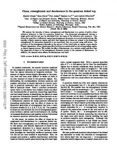
Fig. 2. – Probability density function of the bipartite von Neumann entropy over all balanced bipartitions for the state |ψt i, after 30 iterations of map (46) at K = 1.5. Various histograms are for different numbers of qubits: from left to right nq = 8, 10, 12; dashed curves show the corresponding probabilities for random states. Inset: relative standard deviation σAB /hEAB i as a function of nq (full circles) and best exponential fit σAB /hEAB i ∼ e−0.48 nq (continuous line); data and best exponential fit σAB /hEAB i ∼ e−nq /2 for random states are also shown (empty triangles, dashed line). This figure is taken from Ref. [42].

ity density function p(EAB ) for the entanglement of all possible balanced bipartitions rand of the state |ψt=30 i. This function is sharply peaked around hEAB i, with a relative standard deviation σAB / hEAB i that drops exponentially with nq (see the inset of Fig. 2) and is small (∼ 0.1) already at nq = 4. For this reason, we can conclude that multipartite entanglement is large and that it is reasonable to use the first moment hEAB i of p(EAB ) for its characterization. The corresponding probability densities for random states is also calculated (dashed curves in Fig. 2); their average values and variances are in agreement with the values obtained from states generated by the sawtooth map. As we have remarked in Sec. 3, the fact that for random states the distribution p(EAB ) max is peaked around a mean value close to the maximum achievable value EAB = nq /2 is a manifestation of the concentration of measure phenomenon in a multi-dimensional Hilbert space [40, 18]. 7. – Stability of multipartite entanglement In order to assess the physical significance of the generated multipartite entanglement, it is crucial to study its stability when realistic noise is taken into account. Hereafter I model quantum noise by means of unitary noisy gates, that result from an imperfect control of the quantum computer hardware [55]. The noise model of Ref. [56] is followed. One-qubit gates can be seen as rotations of the Bloch sphere about some fixed

16

G. BENENTI

axis; I assume that unitary errors slightly tilt the direction of this axis by a random amount. Two-qubit controlled phase-shift gates are diagonal in the computational basis; I consider unitary perturbations by adding random small extra phases on all the computational basis states. Hereafter I assume that each noise parameter εi is randomly and uniformly distributed in the interval [−ε, +ε]; errors affecting different quantum gates are also supposed to be completely uncorrelated: every time we apply a noisy gate, noise parameters randomly fluctuate in the (fixed) interval [−ε, +ε]. Starting from a given initial state |ψ0 i, the quantum algorithm for simulating the sawtooth map in presence of unitary noise gives an output state |ψεI ,t i that differs from the ideal output |ψt i. Here εI = (ε1 , ε2 , ..., εnd ) stands for all the nd noise parameters εi , that vary upon the specific noise configuration (nd is proportional to the number of gates). Since we do not have any a priori knowledge of the particular values taken by the parameters εi , the expectation value of any observable A for our nq -qubit system will be given by Tr[ρε,t A], where the density matrix ρε,t is obtained after averaging over noise: (48)

ρε,t =

1 2ε

nd Z

dεI |ψεI ,t ihψεI ,t | .

The integration over εI is estimated numerically by summing over N random realizations of noise, with a statistical error vanishing in the limit N → ∞. The mixed state ρε may also arise as a consequence of non-unitary noise; in this case Eq. (48) can also be seen as an unraveling of ρε into stochastically evolving pure states |ψεI i, each evolution being known as a quantum trajectory [57, 58, 59, 60]. I now focus on the entanglement content of ρε,t . Unfortunately, for a generic mixed state of nq qubits, a quantitative characterization of entanglement is not known, neither unambiguous [2, 3]. Anyway, it is possible to give numerically accessible lower and upper (D) bounds for the bipartite distillable entanglement EAB (ρε ): (49)

(D)

max {S(ρε,A ) − S(ρε ), 0} ≤ EAB (ρε ) ≤ log kρεTB k ,

q where ρε,A = TrB (ρε ) and kρTε B k ≡ Tr (ρTε B )† ρTε B denotes the trace norm of the partial . transpose of ρε with respect to party B (see Appendix A 1 for the definition of the partial transposition operation). In practice, the quantum algorithm for the quantum sawtooth map is simulated in the chaotic regime with noisy gates and the two bounds in Eq. (49) for the bipartite distillable entanglement of the mixed state ρε,t , obtained after averaging over N noise realizations, are evaluated. √ A satisfactory convergence for the lower and the upper bound is obtained after N ∼ N and N ∼ N noise realizations, respectively. The first moment of the lower (Em ) and the upper (EM ) bound for the bipartite distillable entanglement is shown as a function of the imperfection strength in Fig. 3, upper panels. The various curves are for different numbers nq of qubits; N depends on nq and is large enough to obtain negligible statistical errors (smaller than the size of the symbols). The relative standard deviation of the probability density function (over all balanced bipartitions) for the bipartite distillable entanglement is shown in the lower panels of Fig. 3. Like for pure states, we notice an exponential drop with nq ; the distribution width slightly broadens when increasing imperfection strength ε. We can therefore conclude that an average value of the bipartite bipartite distillable entanglement close to the ideal case ε = 0 implies that multipartite entanglement is stable.

17


6

6

Em 5 4

EM 5

3

3

2

2

1

1

0

σm Em

4

0

0.01

0.02

ε

-1

σM EM

10

0

0.01

0.02

ε

0.03

-1

10

-2

10

-2

10

-3

ε = 10 -3 ε = 2.5 10 -3 ε = 5 10 -3

10

0

0.03

-3

ε = 10 -3 ε = 5 10 -2 ε = 10 -3

4

6

8

nq

10

10

4

6

8

nq 10

Fig. 3. – Upper graphs: lower hEm i (left panel) and upper bound hEM i (right panel) for the bipartite distillable entanglement as a function of the noise strength at time t = 30. Various curves stand for different numbers of qubits: nq = 4 (circles), 6 (squares), 8 (diamonds), 10 (triangles up), and 12 (triangles down). Lower graphs: relative standard deviation of the probability density function for distillable entanglement over all balanced bipartitions as a function of nq , for different noise strengths ε. Dashed lines show a behavior σ/ hEi ∼ e−nq /2 and are plotted as guidelines. This figure is taken from Ref. [42].

In order to quantify the robustness of multipartite entanglement with the system size, let us define a perturbation strength threshold ε(R) at which the distillable entanglement bounds drop by a given fraction, for instance to 1/2, of their ε = 0 value, and analyze the behavior of ε(R) as a function of the number of qubits. Numerical results are plotted in Fig. 4; both for lower and upper bounds we obtain a power-law scaling close to (50)

ε(R) ∼ 1/nq .

It is possible to give a semi-analytical proof of the scaling (50) for the lower bound measure, that is based on the quantum Fano inequality [61], which relates the entropy S(ρε ) to the fidelity F = hψt |ρε,t |ψt i: (51)

S(ρε ) . h(F ) + (1 − F ) log(N 2 − 1),

where h(x) = −x log(x) − (1 − x) log(1 − x) is the binary Shannon entropy. Since 2 F ≃ e−γε ng t [56, 62], with γ ∼ 0.28 and ng = 3n2q + nq being the number of gates

18

G. BENENTI

0.028

0.010

εm

εM

(R)

(R)

0.008

t = 15 t = 30

0.020

0.007 0.016

0.006 0.005

0.012

0.004 0.008 0.003

4

8

6

10 12

4

nq

6

8

10 12

nq

Fig. 4. – Perturbation strength at which the bounds of multipartite entanglement halve (lower bound on the left panel, upper bound on the right panel), as a function of the number of qubits. Dashed lines are best power-law fits of numerical data: ε(R) ∼ nq−0.79±0.01 at t = 15, ε(R) ∼ nq−0.9±0.01 at t = 30, for both lower and upper bounds. This figure is taken from Ref. [42].

required for each map step, we obtain, for ε2 ng t ≪ 1, (52)

1 S(ρε ) ≤ γε2 ng t − log(γε2 ng t) + 2nq + . ln 2

For sufficiently large systems the second term dominates (for nq = 12 qubits, t = 30 and ε ∼ 5 × 10−3 the other terms are suppressed by a factor ∼ 1/10) and, to a first approximation, we can only retain it. On the other hand, an estimate of the reduced entropy S(ρA ) is given by the bipartite entropy (47) of a pure random state [16]. Therefore, from Eq. (49) we obtain the following expression for the lower bound of the distillable entanglement: (53)

(D)

EAB (ρε ) ≥ (D)

1 nq − − 6γn3q ε2 t . 2 2 ln 2 (D)

From the threshold definition EAB (ρε(R) ) = 21 EAB (ρ0 ) = 12 S(ρA ) we get the scaling (50), that is valid when nq ≫ 1: (54)

q 2 ε(R) m ∼ 1/ 24 γ nq t.

Notice that, for small systems as the ones that can be numerically simulated (see data in Fig. 4), the first term of Eq. (52) may introduce remarkable logarithmic deviations from the asymptotic power-law behavior. At any rate, the scaling derived from Eq. (53) is in good agreement with the above shown numerical data, and also reproduces the prefactor in front of the power-law decay (50) up to a factor of two.


19

8. – Detecting entanglement of random states The entanglement content of high-dimensional random pure states is almost maximal: nevertheless, in this section I will demonstrate that, due to the complexity of such states, the detection of their entanglement is rather difficult [63]. . 8 1. Random states and the quantum to classical transition. – A motivation to the study of the detection of random states comes from considerations of the quantum to classical transition. Since random states carry a lot of entanglement and entanglement has no analogue in classical mechanics, one can immediately conclude that random states are highly non-classical. On the other hand, as we have seen in Sec. 6, pseudo-random states with properties close to those of true random states can be efficiently generated by dynamical systems (maps) in the regime of quantum chaos. In such chaotic maps the classical limit is recovered when the number of levels N → ∞. Therefore, one can argue that for large random states, i.e., in the limit N → ∞, the quantum expectation value of an operator with a well defined classical limit will be close to its classical microcanonical average. According to this picture random states in a way “mimic” classical microcanonical density. Expectation values are therefore close to the classical ones. At first sight this is in striking contrast with the almost maximal entanglement of such states. However, as I shall discuss in the following, the contradiction is only apparent [63]. The detection of entanglement for a random state appears very difficult at large N , as it would demand the control of very finely interwoven degrees of freedom and a measurement resolution inversely proportional to N , which seems hardly feasible experimentally. Therefore, as far as the detection of entanglement is concerned, high dimensional random states are effectively classical. (10 ) Moreover, coarse graining naturally appears. For instance, one could repeat several times the measurement of an entanglement witness (the definition of entanglement wit. ness is provided in Appendix A 2) for a random state and the prepared random state would be different from time to time due to unavoidable experimental imperfections. Let us model this problem by considering mixtures of m pure random states, namely

(55)

ρ=

m X 1 |ψi ihψi |, m i=1

where the |ψi i are mutually independent random pure states, but in general they are not orthogonal. I am going to show that the detection of entanglement is even more difficult for these mixed states, as it requires a number of measurements growing exponentially with m. It is interesting to remark that there are other physical contexts in which formally the same kind of coarse graining naturally appears: • (i) Time averaging - For example, if a state |ψi undergoes a time evolution |ψ(t)i = U (t)|ψi given in terms of some unitary dynamics U (t), then the time average of a physical observable A over an interval T is given by the expectation value Tr(Aρ) (10 ) Of course, this remark does not call into question the utility of high dimensional random states for quantum information processing.

20

G. BENENTI

for the mixed state (56)

ρ=

1 T

Z

T

dt|ψ(t)ihψ(t)|,

0

which has an effective rank m ≈ T /tcorr , where tcorr is a dynamical correlation time of the dynamics U (t). For a quantum chaotic evolution U (t), the state |ψ(t)i can be, after some time, arguably well described by a random state and the correlation time tcorr is expected to be short, so ρ in Eq. (56) may be well approximated by a mixture of m uncorrelated random states analogous to Eq. (55). • (ii) Phase space averaging - Sometimes it is useful to represent quantum states in terms of distribution functions in the classical phase space, like the Husimi function (see, e.g., [31]), which can be understood as a convolution of the Wigner function or its coarse graining over a phase space volume 2π~ (to simplify writing, let us consider systems with one degree of freedom). In fact, the Husimi function of a pure state can be understood as a Wigner function of the following mixed state: (57)

ρ=

1 2π~

Z

1 dqdp exp − (αq 2 + α−1 p2 ) T (q, p)|ψihψ|T † (q, p), 2~

where T (q, p) are unitary phase space translation operators, and α is an arbitrary (squeezing) parameter. A random pure state |ψi has a Wigner function with random sub-Planck structures with phase space correlation length lcorr ∼ ~ which is semi-classically smaller than the coarse-graining width ∼ ~1/2 , so ρ in Eq. (57) can be again considered as a mixture (Eq. (55)) of m random pure states with m ∼ ~−1/2 . . 8 2. Unknown random states. – In this section is is assumed that the random state |ψi whose entanglement we would like to detect is unknown so that we are not able to use an optimal entanglement witness W for a particular |ψi. The best one can do is to choose some fixed witness W in advance, independently of the state. Since I am interested in the average behavior over unitary invariant ensemble of pure random states, W can be chosen to be random as well. That is, in the present section I am going to study detection of entanglement with a random entanglement witness, whose precise definition will be given later. What I want to calculate is the distribution of the expectation values hψ|W |ψi for a fixed W and an ensemble of random pure states |ψi. Averaging over random states |ψi we see that the average expectation value hψ|W |ψi is (58)

Z

dPhψ|W |ψi = Tr(W )/N,

R where • = dP• denotes an integration over the U (N )-invariant (Haar) P distribution of pure states |ψi, and I used the fact that for a random state |ψi = i ci |ii we have ci c∗j = δij /N . Let us fix normalization of the entanglement witness W such that Tr(W ) = 1. Therefore, the average expectation value hψ|W |ψi scales ∝ 1/N . It is therefore convenient to define the rescaled quantity w = N hψ|W |ψi such that w = 1, independently of the dimension N .


21

Here and in the following, the investigation is limited to decomposable entanglement . witnesses (see Appendix A 2) of the form W = QTB , with Q positive semidefinite operator. I first consider the case when Q is a simple rank one projector, that is,√W is given by W = (|φihφ|)TB . If |φi is a state with a large Schmidt number r ∼ √ N , as it is typical for random |φi (I consider equal size subsystems, NA = NB = N ), then one can show [63] that the probability density p(w) = dP/dw converges to a Gaussian in the limit N → ∞, 1 p(w) = √ exp (−(w − 1)2 /2). 2π

(59)

Numerical results for finite N = 210 are shown in Fig. 5 (top). The probability of R0 measuring negative w, i.e., of detecting entanglement, is −∞ p(w)dw and therefore √ P(w < 0) = (1 − erf(1/ 2))/2 ≈ 0.159.

(60)

Note that this entanglement detection probability is independent of the details of |φi, provided that its Schmidt number r is large, more precisely r ∝ N . Since it appears difficult to measures witness operators corresponding to states |φi with large Schmidt number r, it is interesting to consider the opposite limit of small r. In particular, let us consider the extreme case of rank r = 2. We therefore have only two nonzero terms in the Schmidt decomposition (10), corresponding to the nonzero eigenvalues, p1 = λ and p2 = 1 − λ, of the reduced density matrix ρA = TrB |φihφ| . In this case, we obtain [63]  −w −√ w w 1   (1−2λ) e λ(1−λ) : w > 0, λe λ + (1 − λ)e− 1−λ + √ 1 2 4 λ(1−λ)−2 (61) p(w) = √ w 1  λ(1−λ) √  e : w < 0. 4

λ(1−λ)+2

Results of numerical simulation for p(w) for two cases, λ = 1/2 and λ = 1/26, are compared in in Fig. 5 (bottom). The probability of detecting entanglement, i.e., of measuring negative values of w is p P(w < 0) = 1/(4 + 2/ λ(1 − λ)). (62)

For instance, P(w < 0) = 1/8 = 0.125 when λ = 1/2 and P(w < 0) = 5/72 ≈ 0.07 when λ = 1/26. Note that in the limit λ → 0, i.e., of a pure separable state for |φi, w is always positive with an exponential distribution. I emphasize that, neglecting problems related to finite measurement resolution (an . issue that will be discussed in Sec. 8 3), the entanglement detection probability is, for pure states, independent of the system size N . So far I have discussed only the case when Q is of rank one, Q = |φihφ|. In general, Pk one P can consider Q of rank k: Q = i di |φi ihφi |. Since I have fixed Tr(W ) = 1, then i di = 1. Assuming for simplicity that all di are the same, di = 1/k, we obtain [63], in the limit N → ∞, r k −k(w−1)2 /2 (63) e . p(w) = 2π

22

G. BENENTI

10

0

-1

10

-2

10

-3

10

-4

10

-5

p(w)

10

-4

-2

0

2

4

6

w 10

0

-1

10

-2

10

-3

10

-4

10

-5

p(w)

10

λ=1/2 λ=1/26

-4

-2

0

2

4

6

8

10

12

w TB Fig. 5. – Distribution of w = N hψ|W |ψi for random vectors |ψi and a single W √ = (|φihφ|) √ with a random |φi (top) and with |φi having two nonzero Schmidt coefficients λ and 1 − λ (two cases are shown, λ = 1/2 and λ = 1/26) (bottom). Histograms correspond to numerical simulations for N = 210 , curves to the theoretical predictions of Eqs. (59) (top) and and (61) (bottom). This figure is taken from Ref. [63].

Therefore, the entanglement detection for pure states is more efficient if one consider W = QTB , with Q rank-one projector. It is also interesting to consider the case in which Q is of rank 1 but we wish to detect the entanglement of mixed states, for instance of a mixture of m pure random states, as given in Eq. (55). In this case, the resulting distribution p(w) is, in the limit N → ∞, a Gaussian of variance 1/m [63]. Because the distribution p(w) becomes narrowly peaked about its mean w = 1 with increasing m, the probability of measuring negative values


23

decreases with m, that is, we obtain (64)

p 1 − erf( m/2) 1 ≍√ e−m/2 . P(w < 0) = 2 2πm

This probability decays to zero exponentially with m. Therefore, the detection of entanglement for a mixture of random states is very hard. This result outlines the importance of coarse graining to explain the emergence of classicality. For random pure states, a finite success probability in the detection of entanglement exists also in the limit in which the Hilbert space dimension N → ∞. This implies that chaotic dynamics alone is not sufficient to erase any trace of entanglement when going to the classical limit, provided that ideal measurements are possible. On the other hand such erasure becomes very efficient when coarse graining is taken into account, for instance when mixtures instead of pure states are considered. . 8 3. Known random states. – In this section it is assumed that the random state |ψi whose entanglement we want to measure is known in advance and furthermore, that we are able to prepare an arbitrary decomposable entanglement witness. In addition, we have to assume that our state |ψi is neither separable, nor bound entangled (see Appendix A), which is true with probability which converges to one exponentially in N . Therefore, for each |ψi we can prepare an optimal entanglement witness, such that its expectation value will be minimal. As far as decomposable entanglement witnesses are concerned, the optimal choice of W = Wopt is to take for Q a projector to the eigenspace corresponding to the minimal (negative) eigenvalue λmin of ρTB , Wopt = (|φmin ihφmin |)TB . The maximal violation of positivity is therefore (65)

Tr(Wopt ρ) = −|λmin (ρTB )|.

If we are able to measure the entanglement witness Wopt with a given precision it is the size of λmin which determines the difficulty of detecting entanglement in |ψi. Note that the optimal entanglement witness Wopt depends on the state |ψi. For each state |ψi we have to pick a different Wopt . √ The expectation value of the minimal eigenvalue equals λmin √= −4/ N [63]. In fact, the distribution of λmin becomes strongly peaked around −4/ N with diminishing relative fluctuations as N → ∞.PWhen we mix several independent (in general nonm orthogonal) random vectors, ρ = i |ψi ihψi |/m, the minimal eigenvalue λmin increases and the distribution becomes increasingly sharply peaked (for m → ∞ we get ρ → 1/N ¯ min with all eigenvalues being equal to 1/N ). Note that the average minimal eigenvalue λ ∗ ∗ is positive for m > m , with m ≈ 4N . Although von Neumann entropy of a random state is large all eigenvalues of ρTB are very small and will therefore be hard to detect. If we assume that we are able to measure values of |Tr(W ρ)| < ǫ then we can, depending on the scaling of ǫ with N , tell for which values of m the detection of entanglement is possible. If ǫ does not depend on√N , i.e., precision does not increase with N , then for sufficiently large N , such that 4/ N < ǫ, detection of entanglement will be impossible. Already a single random state becomes from the viewpoint of entanglement detection “classical”, since measuring a negative expectation value of its optimal entanglement witness is below the √ detection limit. If on the other hand we are able to measure ǫ which decreases as 1/ N , the critical mcrit , beyond which the entanglement detection is impossible, will be independent of N , i.e.,

24

G. BENENTI

√ in the limit N → ∞ the ratio mcrit / N → 0. If however we are able to detect very small expectation values of order 1/N , then mcrit will be proportional to N . Furthermore, even with arbitrary accuracy, detection of entanglement with decomposable entanglement ¯ min becomes witnesses is in practice impossible beyond m = m∗ ∝ N (that is, when λ positive). I would like to stress once more than the detection difficulties are a consequence of the complexity of random states. If instead one considers “regular states” such as the GHZ state [44] |GHZi = √12 (|0...0i + |1...1i), then the optimal witness is Wopt = (|φmin ihφmin |)TB , with |φmin i = √12 (|0...0i|1...1i − |1...1i|0...0i) which corresponds to the minimal eigenvalue λmin = −1/2 of (|GHZihGHZ|)TB . Since the value of λmin is −1/2 √ instead of −4/ N as typical for a random state, it turns out that it will be much easier to detect entanglement in a “regular” rather than in a random state. This happens in spite of the fact that the entanglement content is much larger in a random than in such a regular state.

9. – Chaotic environments Real physical systems are never isolated and the coupling of the system to the environment leads to decoherence. This process can be understood as the loss of quantum information, initially present in the state of the system, when non-classical correlations (entanglement) establish between the system and the environment. On the other hand, when tracing over the environmental degrees of freedom, we expect that the entanglement between internal degrees of freedom of the system is reduced or even destroyed. Decoherence theory has a fundamental interest, since it provides explanations of the emergence of classicality in a world governed by the laws of quantum mechanics [64]. Moreover, it is a threat to the actual implementation of any quantum computation and communication protocol [7, 8]. Indeed, decoherence invalidates the quantum superposition principle, which is at the heart of the power of quantum algorithms. A deeper understanding of the decoherence phenomenon is essential to develop quantum technologies. The environment is usually described as a many-body quantum system. The bestknown model is the Caldeira-Leggett model [65, 66, 67], in which the environment is a bosonic bath consisting of infinitely many harmonic oscillators at thermal equilibrium. More recently, first studies of the role played by chaotic dynamics [68, 69, 70, 71, 72, 73] or random environments [74, 75] in the decoherence process have been carried out. In the following, it is shown that the many-body environment may be substituted with a closed deterministic system with a small number of degrees of freedom, but chaotic [72]. In other words, the complexity of the environment arise not from being many-body but from having chaotic dynamics. I consider two qubits coupled to a single particle, fully deterministic, conservative chaotic “environment”, described by the kicked rotator model. It is shown that, due to the system-environment interaction, the entropy of the system increases. At the same time, the entanglement between the two qubits decays, thus illustrating the loss of quantum coherence. The evolution in time of the two-qubit entanglement is in good agreement with the evolution obtained in a pure dephasing stochastic model. Since this pure dephasing decoherence mechanism can be derived in the framework of the Caldeira-Leggett model [76], a direct link between the effects of a many-body environment and of a chaotic single-particle environment is established. Let us consider two qubits coupled to a quantum kicked rotator. The overall system

25


is governed by the Hamiltonian (66)

ˆ =H ˆ (1) + H ˆ (2) + H ˆ (kr) + H ˆ (int) , H

(i) ˆ (i) = ωi σ where H ˆx (i = 1, 2) describes the free evolution of the two qubits,

(67)

X ˆ2 ˆ ˆ (kr) = n δ(τ − jT ) + k cos(θ) H 2 j

the quantum kicked rotator, and (68)

ˆ ˆ (int) = ǫ (ˆ H σz(1) + σ ˆz(2) ) cos(θ)

X j

δ(τ − jT ) (i)

the interaction between the qubits and the kicked rotator; as usual, σ ˆα (α = x, y, z) ˆ (kr) and the denote the Pauli operators for the i-th qubit. Both the cosine potential in H (int) ˆ interaction H are switched on and off instantaneously (kicks) at regular time intervals T . Let us consider the two qubits as an open quantum system and the kicked rotator as their common environment. Note that I chose non-interacting qubits as I want their entanglement to be affected exclusively by the coupling to the environment (11 ) The kicked rotator, as the sawtooth map described in detail in Appendix C, belongs to the class of periodically driven systems of Eq. (C.1), with the external driving described by the potential V (θ) = k cos θ, switched on and off instantaneously at time intervals T . The evolution from time tT − (prior to the t-th kick) to time (t + 1)T − (prior to the (t + 1)-th kick) of the kicked rotator in the classical limit is described by the Chirikov standard map: (69)

nt+1 = nt + k sin θt , θt+1 = θt + T nt+1 ,

where (n, θ) are conjugated momentum-angle variables and t = τ /T denotes the discrete time, measured in number of kicks. As for the sawtooth map, by rescaling n → p = T n, the dynamics of Eq. (69) is seen to depend only on the parameter K = kT . For K = 0 the motion is integrable; when K increases, a transition to chaos of the Kolmogorov-ArnoldMoser (KAM) type is observed [79, 80]. (12 ) The last invariant KAM torus is broken for K ≈ 0.97. If K ∼ 1 the phase space is mixed (simultaneous presence of integrable and chaotic components). If K increases further, the stability islands progressively reduce their size; for K ≫ 1 they are not visible any more. In what follows, I always consider (11 ) As discussed in [70], the chaotic environment model discussed in this section could be implemented, at least in principle, using cold atoms in a pulsed optical lattice created by laser fields [77] or superconducting nanocircuits [78]. (12 ) The property of complete integrability is very delicate and atypical as it is, in general, destroyed by an arbitrarily weak perturbation that converts a completely integrable system into a KAM-integrable system. The structure of KAM motion is very intricate: the motion is confined to invariant tori for most initial conditions yet a single, connected, chaotic motion component (for more than two degrees of freedom) of exponentially small measure (with respect to the perturbation) arises, which is nevertheless everywhere dense.

26

G. BENENTI

map (69) on the torus 0 ≤ θ < 2π, −π ≤ p < π. In this case, the Chirikov standard map describes the stroboscopic dynamics of a conservative dynamical system with two degrees of freedom which, in the fully chaotic regime K ≫ 1, relaxes, apart from quantum fluctuations, to the uniform distribution on the torus. The Hilbert space of the global system is given by (70)

H = H(1) ⊗ H(2) ⊗ H(kr) ,

where H(1) and H(2) are the two-dimensional Hilbert spaces associated to the two qubits, and H(kr) is the Hilbert space for the kicked rotator with N quantum levels. The time evolution generated by Hamiltonian (66) in one kick is described by the operator (71)

(1) (2) ˆ ˆ = exp − i k + ǫ(ˆ U σz + σ ˆz ) cos(θ) 2 (1) (2) ˆx exp − i δ2 σ ˆx . × exp − iT nˆ2 exp − i δ1 σ

The effective Planck constant is ~eff = T = 2π/N ; δ1 = ω1 T, δ2 = ω2 T ; ǫ is the coupling strength between the qubits and the environment. The classical limit ~eff → 0 is obtained by taking T → 0 and k → ∞, in such a way that K = kT is kept fixed. I am interested in the case in which the environment (the kicked rotator) is chaotic (that is, with K ≫ 1). The two qubits are initially prepared in a maximally entangled state, so that they are disentangled from the environment. Namely, I suppose that at t = 0 the system is in the state (72)

|Ψ0 i = |φ+ i ⊗ |ψ0 i ,

where |φ+ i = √12 (|00i + |11i) is a Bell state (the particular choice of the initial maximally P entangled state is not crucial for what follows), and |ψ0 iP = n cn |ni is a generic state of the kicked rotator, with cn random coefficients such that n |cn |2 = 1, and |ni eigenstates of the momentum operator. The evolution in time of the global system (kicked rotator ˆ defined in Eq. (71). Therefore, any plus qubits) is described by the unitary operator U ˆ t |Ψ0 i. The reduced initial pure state |Ψ0 i evolves into another pure state |Ψ(t)i = U density matrix ρ12 (t) describing the two qubits at time t is then obtained after tracing |Ψ(t)ihΨ(t)| over the kicked rotator’s degrees of freedom. In the following I will focus my attention on the time evolution of the entanglement of formation (see Appendix D) E12 between the two qubits and that between them and the kicked rotator, measured by the reduced von Neumann entropy S12 = −Tr [ρ12 log2 ρ12 ] of the reduced density matrix ρ12 . Clearly, for states like the one in Eq. (72), we have E12 (0) = 1, S12 (0) = 0. As the total system evolves, we expect that E12 decreases, while S12 grows up, thus meaning that the two-qubit system is progressively losing coherence. If the kicked rotator is in the chaotic regime and in the semiclassical region ~eff ≪ 1, it is possible to drastically simplify the description of the system in Eq. (66) by using the random phase-kick approximation, in the framework of the Kraus representation formalism. Since, to a first approximation, the phases between two consecutive kicks in the chaotic regime can be considered as uncorrelated, the interaction with the environment can be simply modeled as a phase-kick rotating both qubits through the same random angle about the z-axis of the Bloch sphere. This rotation is described in the

27


2

S12 1.5 0

10

E12

1

10

10

-1

-2

0.5 -3

10 0

0

0

4

1×10

4

1×10 4

4

2×10 4

2×10

3×10

4

4

3×10

t

4×10

4

4×10

4

5×10

t

Fig. 6. – Reduced von Neumann entropy S12 √ (main figure) and entanglement E12 (inset) as a function of time at K ≈ 99.73, δ1 = 10−2 , δ2 = 2δ1 , ǫ = 8×10−3 . The thin curves correspond to different number of levels for the environment (the kicked rotator) (N = 29 , 210 , 211 , 212 , 213 , 214 from bottom to top in the main figure and vice versa in the inset). The thick curves give the numerical results from the random phase model (74).

{|00i, |01i, |10i, |11i} basis by the unitary matrix (73)

R(θ) =

e−iǫ cos θ 0

0 eiǫ cos θ

⊗

e−iǫ cos θ 0

0 eiǫ cos θ

,

where the angle θ is drawn from a uniform random distribution in [0, 2π). The one-kick evolution of the reduced density matrix ρ12 is then obtained after averaging over θ: (74)

ρ¯12 =

1 2π

Z

2π

(2)

(1)

(1)

(2)

dθ R(θ) e−iδ2 σx e−iδ1 σx ρ12 eiδ1 σx eiδ2 σx R† (θ).

0

In order to assess the validity of the random phase-kick approximation, model (66) is numerically investigated in the classically chaotic regime K ≫ 1 and in the region ~eff ≪ 1 in which the environment is a semiclassical object. Under these conditions, we expect that the time evolution of the entanglement can be accurately predicted by the random phase model. Such expectation is confirmed by the numerical data shown in Fig. 6. Even though differences between the two models remain at long times due to the finite number N of levels in the kicked rotator, such differences appear at later and later times when N → ∞ (~eff → 0). The parameter K has been chosen much greater than one, so that the classical phase space of the kicked rotator can be considered as completely chaotic. Note that the value K ≈ 99.72676 is chosen to completely wipe off memory effects between consecutive and next-consecutive kicks (see Ref. [72] for details).

28

G. BENENTI

I point out that the random phase model can be derived from the Caldeira-Leggett (1) (2) P model with a pure dephasing coupling ∝ (ˆ σz + σ ˆz ) k gk qˆk , with gk coupling constant to the k-th oscillator of the environment, whose coordinate operator is qˆk [76, 81]. This establishes a direct link between the chaotic single-particle environment considered in this paper and a standard many-body environment. 10. – Final remarks The role of entanglement as a resource in quantum information has stimulated intensive research aimed at unveiling both its qualitative and quantitative aspects. The interest is first of all motivated by experimental implementations of quantum information protocols. Decoherence, which can be considered as the ultimate obstacle in the way of actual implementation of any quantum computation or communication protocol, is due to the entanglement between the quantum hardware and the environment. The decoherence-control issue is expected to be particularly relevant when the state of the quantum system is complex, namely when it is characterized by a large amount of multipartite entanglement. It is therefore important, for applications but also in its own right, to scrutinize the robustness and the multipartite features of relevant classes of entangled states. In this context, random states play an important role, both for applications in quantum protocols and in view of a, highly desirable, statistical theory of entanglement. Such studies have deep links with the physics of complex systems. In classical physics, a well defined notion of complexity, based on the exponential instability of chaos, exists, and has profound links with the notion of algorithmic complexity [82, 83]: in terms of the symbolic dynamical description, almost all orbits are random and unpredictable. On the other hand, in spite of many efforts (see [84] and references therein) the transfer of these concepts to quantum mechanics still remains elusive. However, there is strong numerical evidence that quantum motion is characterized by a greater degree of stability than classical motion (see [85, 36, 7, 86]). This has important consequences on the stability of quantum algorithms; for instance, the robustness of the multipartite entanglement generated by chaotic maps and discussed in Sec. 7 is related to the power-law decay of the fidelity time scales for quantum algorithms [87, 88, 54, 89] which, in turn, is a consequence of the discreteness of the phase space in quantum mechanics [85, 36, 7, 86]. If we consider the chaotic classical motion (governed by the Liouville equation) of some phase-space density, smaller and smaller scales are explored exponentially fast. These fine details of the density distribution are rapidly lost under small perturbations. In quantum mechanics, there is a lower limit to this process, set by the size of the Planck cell, and this reduces the complexity of quantum motion as compared to classical motion. Finally, the fundamental, purely quantum notion of entanglement is expected to play a crucial role in characterizing the complexity of a quantum system [90]. I believe that studies of complexity and multipartite entanglement will shed some light on series of very important issues in quantum computation and in critical phenomena of quantum many-body condensed matter physics. Appendix A. Separability criteria . A 1. The Peres criterion. – The Peres criterion [91] provides a necessary condition for the existence of decomposition (17), in other words, a violation of this criterion is

29


a sufficient condition for entanglement. This criterion is based on the partial transpose operation. Introducing an orthonormal basis {|iiA |αiB } in the Hilbert space HAB associated with the bipartite system A + B, the density matrix ρAB has matrix elements (ρAB )iα;jβ = A hi|B hα|ρAB |jiA |βiB . The partial transpose density matrix is constructed by only taking the transpose in either the Latin or Greek indices (here Latin indices refer to Alice’s subsystem and Greek indices to Bob’s). For instance, the partial transpose with respect to Alice is given by (A.1)

A ρTAB

iα;jβ

= ρAB

jα;iβ

.

Since a separable state ρAB can always be written in the form (17) and the density matrices ρAk and ρBk have non-negative eigenvalues, then the overall density matrix ρAB also has non-negative eigenvalues. The partial transpose of a separable state reads (A.2)

A ρTAB =

X k

pk ρTAk ⊗ ρBk .

Since the transpose matrices ρTAk = ρ⋆Ak are Hermitian non-negative matrices with unit trace, they are also legitimate density matrices for Alice. It follows that none of the A eigenvalues of ρTAB is non-negative. This is a necessary condition for decomposition (17) A to hold. It is then sufficient to have at least one negative eigenvalue of ρTAB to conclude that the state ρAB is entangled. It can be shown [92] that for composite states of dimension 2 × 2 and 2 × 3, the Peres criterion provides a necessary and sufficient condition for separability; that is, the state A ρAB is separable if and only if ρTAB is non-negative. However, for higher dimensional systems, states exist for which all eigenvalues of the partial transpose are non-negative, but that are non-separable [93]. These states are known as bound entangled states since they cannot be distilled by means of local operations and classical communication to form a maximally entangled state [94]. I stress that the Peres criterion is more sensitive than Bell’s inequality for detecting quantum entanglement; that is, there are states detected as entangled by the Peres criterion that do not violate Bell’s inequalities ([91]). . A 2. Entanglement witnesses. – A convenient way to detect entanglement is to use the so-called entanglement witnesses [92, 95]. By definition, an entanglement witness is (sep) (sep) a Hermitian operator W such that Tr W ρAB ≥ 0 for all separable states ρAB while (ent) (ent) there exists at least one state ρAB such that Tr W ρAB ) < 0. Therefore, the negative (ent) expectation value of W is a signature of entanglement and the state ρAB is said to be detected as entangled by the witness W . The existence of entanglement witnesses is a consequence of the Hahn-Banach theorem: Given a convex and compact set S and ρAB ∈ / S, there exists a hyperplane that separates ρAB from S. This fact is illustrated in Fig. 7. The set S of separable states is a subset of the set of all possible density matrices for a given system. The dashed line represents a hyperplane separating an entangle state ρAB from S. The optimized witness Wopt (represented by a full line) is obtained after performing a parallel transport of the above hyperplane, so that it becomes tangent to the set of separable states. Therefore, the optimized witness Wopt detects more entangled states than before parallel transport. Note that, in order to fully characterize the set S of separable states one should find all the witnesses tangent to S.

30

G. BENENTI

E

ρAB W W opt

S

Fig. 7. – Schematic drawing of entanglement witnesses.

The concept of entanglement witness is close to experimental implementations and detection of entanglement by means of entanglement witnesses has been realized in several experiments [96, 97, 98]. The more negative expectation value of entanglement witness we find, the easier it is to detect entanglement of such a state. The expectation value of W also provides lower bounds to various entanglement measures [99, 100]. Finally, it is interesting to note that violation of Bell’s inequalities can be rewritten in terms of non-optimal entanglement witnesses [95, 101]. In general, classification of entanglement witnesses is a hard problem. However, much simpler is the issue with the so-called decomposable entanglement witnesses [102]. By definition, a witness is called decomposable if (A.3)

W = P + QTB ,

P, Q ≥ 0,

that is, with positive semidefinite operators P, Q. Decomposable entanglement witnesses can only detect entangled states with at least one negative eigenvalues of ρTB . Therefore, similarly to the Peres criterion, decomposable witnesses do not detect bound entangled states. Note, however, that entanglement witnesses are closer to experimental implementations than the Peres criterion, as full tomographic knowledge about the state is not needed. Appendix B. Purity of random states Let us write a N -level random state in the form (B.1)

|ψi =

N −1 X k=0

rk eiφk |ki,

31


where φk are independent random variables uniformly distributed in [0, 2π) and r = (r0 , ..., rN −1 ) is a random point uniformly distributed on the unit hypersphere SN −1 = {r ∈ RN |r2 = 1}, with distribution function p(r) = CN

(B.2)

N −1 Y k=0

rk δ(r2 − 1),

with CN normalization constant to be determined later. Given a bipartition of the Hilbert space of the system into two parts, A and B, with dimensions NA and NB , the purity reads (B.3)

P =

NX A −1 NX B −1 j,j ′ =0 l,l′ =0

rjl rj ′ l rj ′ l′ rjl′ exp[i(φjl − φj ′ l + φj ′ l′ − φjl′ )],

where |ki = |jli = |jiA ⊗ |liB . Following [43], I split P in two parts: (B.4)

P = X + M,

where (B.5)

X=

X X ′

j,j ′

(B.6)

l,l′

M=

′

rjl rj ′ l rj ′ l′ rjl′ exp[i(φjl − φj ′ l + φj ′ l′ − φjl′ )],

X X ′

j,j ′

2 2 rjl rj ′ l +

XX j

l

′ 2 2 rjl rjl′

l,l′

+

X

4 rjl ,

j,l

P′ means that equal indexes are banned in the sum. Since heiφk i = 0 we obtain where hXi = 0. Therefore, (B.7)

P = hM i = N (NA + NB − 2)hr02 r12 i + N hr04 i,

where I have used hrk4 i = hr04 i for all k and hrk2 rk2′ i = hr02 r12 i for all k, k ′ with k 6= k ′ . I now evaluate the marginal distribution p(r0 , ..., rm−1 ) = CN r0 · · · rm−1

CN r0 · · · rm−1 = 2

(B.8)

Z

1

drm rm

0

Z √1−r02 −...−rm−1 2 0

Z

0

1

drm+1 rm+1 · · ·

drm rm · · ·

Z

0

1

drN −1 rN −1 δ(r2 − 1)

Z √1−r02 −...−rN 2 −3 0

drN −2 rN −2

N −m−1  m−1 X 1 rj2  r0 · · · rm−1 1 − . = N −m 2 (N − m − 1)! j=0 CN

32

G. BENENTI

In particular, (B.9)

1 CN r0 (1 − r02 )N −2 . 2N −1 (N − 2)!

p(r0 ) = R1

The normalization condition Thus, we obtain

0

dr0 p(r0 ) = 1 allows us to determine CN = 2N (N − 1)!.

p(r0 ) = 2(N − 1)r0 (1 − r02 )N −2 ,

(B.10)

hr04 i =

(B.11)

Z

0

1

dr0 r04 p(r0 ) =

2 , N (N + 1)

(B.12)

p(r0 , r1 ) = 4(N − 1)(N − 2)r0 r1 (1 − r02 − r12 )N −3 ,

(B.13)

hr02 r12 i =

Z

0

1

dr0 r02

Z

0

1

dr1 r12 p(r0 , r1 ) =

1 . N (N + 1)

After substitution of Eqs. (B.11) and (B.13) into (B.7) we readily obtain Lubkin’s formula (23). The variance σP2 can be computed with the same technique as above [43, 35]. However, to obtain the variance (24) √ for large N it is suffcient to replace in Eqs. (B.5) and (B.6) rk with its mean value 1/ N : (B.14)

σP2 = hP 2 i − PL2 = hX 2 i + hM 2 i − PL2 ≈ hX 2 i ≈

2 . N2

We can see from Eqs. (B.5) and (B.6) that X and M are sums of O(N 2 ) terms of order 1/N 2 . Therefore, the central limit theorem implies that, for large N , the purity tends to a Gaussian distribution with mean PL and variance σP . Finally, I note that all moments of the purity have been recently computed [103].

Appendix C. The sawtooth map The sawtooth map is a prototype model in the studies of classical and quantum dynamical systems and exhibits a rich variety of interesting physical phenomena, from complete chaos to complete integrability, normal and anomalous diffusion, dynamical localization, and cantori localization. Furthermore, the sawtooth map gives a good approximation to the motion of a particle bouncing inside a stadium billiard (which is a well-known model of classical and quantum chaos).

33


. C 1. Classical dynamics. – The sawtooth map belongs to the class of periodically driven dynamical systems, governed by the Hamiltonian (C.1)

H(θ, n; τ ) =

+∞ X n2 δ(τ − jT ) , + V (θ) 2 j=−∞

where (n, θ) are conjugate action-angle variables (0 ≤ θ < 2π). This Hamiltonian is the sum of two terms, H(θ, n; τ ) = H0 (n) + U (θ; τ ), where H0 (n) = n2/2 is just the kinetic energy of a free rotator (a particle moving on a circle parametrized by the coordinate θ), while X (C.2) δ(τ − jT ) U (θ; τ ) = V (θ) j

represents a force acting on the particle that is switched on and off instantaneously at time intervals T . Therefore, we say that the dynamics described by Hamiltonian (C.1) is kicked. The corresponding Hamiltonian equations of motion are

(C.3)

 +∞ ∂H dV (θ) X    n˙ = − δ(τ − jT ) , =− ∂θ dθ j=−∞    θ˙ = ∂H = n . ∂n

These equations can be easily integrated and one finds that the evolution from time tT − (prior to the t-th kick) to time (t + 1)T − (prior to the (t + 1)-th kick) is described by the map (C.4)

(

nt+1 = nt + F (θ) , θt+1 = θt + T nt+1 ,

where the discrete time t = τ /T measures the number of map iterations and F (θ) = −dV (θ)/dθ is the force acting on the particle. In the following, we focus on the special case V (θ) = −k(θ − π)2 /2. This map is called the sawtooth map, since the force F (θ) = −dV (θ)/dθ = k(θ − π) has a sawtooth shape, with a discontinuity at θ = 0. For such a discontinuous map the conditions of the Kolmogorov-Arnold-Moser (KAM) theorem are not satisfied and, for any k 6= 0, the motion is not bounded by KAM tori. By rescaling n → I = T n, the classical dynamics is seen to depend only on the parameter K = kT . Indeed, in terms of the variables (I, θ) map (C.4) becomes (C.5)

(

It+1 = It + K(θ − π) , θt+1 = θt + It+1 .

The sawtooth map exhibits sensitive dependence on initial conditions, which is the distinctive feature of classical chaos: any small error is amplified exponentially in time. In other words, two nearby trajectories separate exponentially, with a rate given by the maximum Lyapunov exponent λ, defined as 1 δt λ = lim (C.6) , ln |t|→∞ t δ0

34

where δt = ing (C.7)

G. BENENTI

p [δIt ]2 + [δθt ]2 . To compute δIt and δθt , we differentiate map (C.5), obtain

δIt+1 δθt+1

=M

δIt δθt

=

1 K 1 1+K

δIt δθt

.

The iteration of map (C.7) gives δIt and δθt as a function of δI0 and δθ0 (δI0 and δθ0 represent a change √ of the initial conditions). The stability matrix M has eigenvalues µ± = 21 (2 + K ± K 2 + 4K), which do not depend on the coordinates I and θ and are complex conjugate for −4 ≤ K ≤ 0 and real for K < −4 and K > 0. Thus, the classical motion is stable for −4 ≤ K ≤ 0 and completely chaotic for K < −4 and K > 0. For K > 0, δt ∝ (µ+ )t asymptotycally in t, and therefore the maximum Lyapunov exponent is λ = ln µ+ . Similarly, we obtain λ = ln |µ− | for K < −4. In the stable region −4 ≤ K ≤ 0, λ = 0. The sawtooth map can be studied on the cylinder [I ∈ (−∞, +∞)], or on a torus of sinite size (−πL ≤ I < πL, where L is an integer, to assure that no discontinuities are introduced in the second equation of (C.5) when I is taken modulus 2πL). Although the sawtooth map is a deterministic system, for K > 0 and K < −4 the motion along the momentum direction is in practice indistinguishable from a random walk. Thus, one has normal diffusion in the action (momentum) variable and the evolution of the distribution function f (I, t) is governed by a Fokker–Planck equation:

∂f ∂ = ∂t ∂I

(C.8)

1 ∂f D 2 ∂I

.

The diffusion coefficient D is defined by h(∆It )2 i , t→∞ t

D = lim

(C.9)

where ∆I ≡ I − hIi, and h. . .i denotes the average over an ensemble of trajectories. If at time t = 0 we take a phase space distribution with initial momentum I0 and random phases 0 ≤ θ < 2π, then the solution of the Fokker–Planck equation (C.8) is given by 1 (I − I0 )2 f (I, t) = √ . exp − 2Dt 2πDt

(C.10) The width (C.11)

p h(∆It )2 i of this Gaussian distribution grows in time, according to h(∆It )2 i ≈ D(K) t .

For K > 1, the diffusion coefficient is well approximated by the random phase approximation, in which we assume that there are no correlations between the angles (phases) θ at different times. Hence, we have 1 (C.12)D(K) ≈ h(∆I ) i = 2π (1 2

Z

0

2π

dθ(∆I

1 ) = 2π

(1) 2

Z

0

2π

dθK 2 (θ − π)2 =

π2 2 K , 3

where ∆I (1) = It+1 − It is the change in action after a single map step. For 0 < K < 1 diffusion is slowed, due to the sticking of trajectories close to broken tori (known as

35


cantori), and we have D(K) ≈ 3.3 K 5/2 (this regime is discussed in Ref. [104]). For −4 < K < 0 the motion is stable, the phase space has a complex structure of elliptic islands down to smaller and smaller scales, and one can observe anomalous diffusion, that is, h(∆J)2 i ∝ tα , with α 6= 1 (see Ref. [54]). The cases K = −1, −2, −3 are integrable. . C 2. Quantum dynamics. – The quantum version of the sawtooth map is obtained by means of the usual quantization rules, θ → θˆ and n → n ˆ = −i∂/∂θ (we set ~ = 1). The ˆ , called the quantum evolution in one map iteration is described by a unitary operator U Floquet operator, acting on the wave vector |ψi: (C.13)

"

ˆ |ψit = exp −i |ψit+1 = U

Z

(l+1)T −

lT −

#

ˆ I; ˆ τ ) |ψit , dτ H(θ,

where H is Hamiltonian (C.1). Since the potential V (θ) is switched on only at discrete times lT , it is straightforward to obtain (C.14)

2

ˆ

|ψit+1 = e−iT nˆ /2 e−iV (θ) |ψit ,

which for the sawtooth map is just Eq. (46). It is important to emphasize that, while the classical sawtooth map depends only on the rescaled parameter K = kT , the corresponding quantum evolution (C.14) depends on k and T separately. The effective Planck constant is given by ~eff = T . Indeed, if we consider the operator Iˆ = T n ˆ (Iˆ is the quantization of the classical rescaled action I), we have (C.15)

ˆ I] ˆn ˆ = T [θ, [θ, ˆ ] = iT = i~eff .

The classical limit ~eff → 0 is obtained by taking k → ∞ and T → 0, while keeping K = kT constant. In the quantum sawtooth map model one can observe important physical phenomena like dynamical localization [105]. Indeed, due to quantum interference effects, the chaotic diffusion in momentum is suppressed, leading to exponentially localized wave functions. This phenomenon was first found and studied in the quantum kicked-rotator model [106] and has profound analogies with Anderson localization of electronic transport in disordered materials [107]. Dynamical localization has been observed experimentally in the microwave ionization of Rydberg atoms [108] and in experiments with cold atoms [109]. In the quantum sawtooth map also cantori localization takes place: In the vicinity of a broken KAM torus, a cantorus starts to act as a perfect barrier to quantum wave packet evolution, if the flux through it becomes less than ~ [110, 111, 112, 113, 114]. . C 3. Quantum algorithm. – In the following, we describe an exponentially efficient quantum algorithm for simulation of the map (46) [54]. It is based on the forward/ backward quantum Fourier transform between momentum and angle bases. Such an ˆ , introduced in Eq. (46), is the approach is convenient since the Floquet operator U 2 2 ˆ ik(θ−π) /2 ˆ ˆ product of two operators, Uk = e and UT = e−iT nˆ /2 , diagonal in the θ and n representations, respectively. This quantum algorithm requires the following steps for one map iteration: ˆk to the wave function ψ(θ). In order to decompose the operator U ˆk into • Apply U

36

G. BENENTI

one- and two-qubit gates, we first of all write θ in binary notation: (C.16)

θ = 2π

nq X

αj 2−j ,

j=1

with αi ∈ {0, 1}. Here nq is the number of qubits, so that the total number of levels in the quantum sawtooth map is N = 2nq . From this expansion, we obtain (θ − π)2 = 4π 2

(C.17)

nq X αj2 1 1 αj1 . − − 2j1 2n 2j2 2n j ,j =1 1

2

ˆk , giving the decomposition This term can be put into the unitary operator U (C.18)

2

eik(θ−π) /2 =

n Y

j1 ,j2

αj2 αj1 1 1 , exp i2π 2 k − − 2j1 2n 2j2 2n =1

which is the product of n2q two-qubit gates (controlled phase-shift gates), each acting non-trivially only on the qubits j1 and j2 . In the computational basis {|αj1 αj2 i = |00i, |01i, |10i, |11i} each two-qubit gate can be written as exp(i2π 2 kDj1 ,j2 ), where Dj1 ,j2 is a diagonal matrix: 

 (C.19) Dj1 ,j2 =  

1 4n2

0 0 0

0 1 − 2n

1 2j2

0 0

−

1 2n

0 0 1 − 2n

1 2j1

0

−

1 2n

1 2j1

−

1 2n

0 0 0

 1 2j2

−

1 2n

 . 

• The change from the θ to the n representation is obtained by means of the quantum Fourier transform, which requires nq (single-qubit) Hadamard gates and 12 nq (nq −1) (two-qubit) controlled phase-shift gates (see, e.g., [7, 8]). ˆT has essentially the same form as the oper• In the n representation, the operator U ˆ ator Uk in the θ representation and can therefore be decomposed into n2q controlled phase-shift gates, similarly to Eq. (C.18). • Return to the initial θ representation by application of the inverse quantum Fourier transform. Thus, overall, this quantum algorithm requires 3n2q +nq gates per map iteration (3n2q −nq controlled phase-shifts and 2nq Hadamard gates). This number is to be compared with the O(nq 2nq ) operations required by a classical computer to simulate one map iteration by means of a fast Fourier transform. Thus, the quantum simulation of the quantum sawtooth map dynamics is exponentially faster than any known classical algorithm. Note that the resources required to the quantum computer to simulate the evolution of the sawtooth map are only logarithmic in the system size N . Of course, there remains the problem of extracting useful information from the quantum computer wave function. For a discussion of this problem, see Refs. [7, 115]. Finally, I point out that the quantum sawtooth map has been recently implemented on a three-qubit nuclear magnetic resonance (NMR)-based quantum processor [116].

37


Appendix D. Entanglement of formation and concurrence Any state ρ can be decomposed as a convex combination of projectors onto pure states: X (D.1) pj |ψj ihψj |. ρ= j

The entanglement of formation E is defined as the mean entanglement of the pure states forming ρ, minimized over all possible decompositions: (D.2)

E(ρS ) = inf

dec

X j

pj E(|ψj i),

where the (bipartite) entanglement of the pure states |ψj i is measured according to Eq. (9). The entanglement of formation E12 of a generic two-qubit state ρ12 can be evaluated in a closed form following Ref. [117]. First of all we compute the concurrence, defined as C = max(λ1 − λ2 − λ3 − λ4 , 0), where the λi ’s are the square roots of the eigenvalues of the matrix R = ρ12 ρ˜12 , in decreasing order. Here ρ˜12 is the spin flipped matrix of ρ12 , and it is defined by ρ˜12 = (σy ⊗ σy ) ρ⋆12 (σy ⊗ σy ) (note that the complex conjugate is taken in the computational basis {|00i, |01i, |10i, |11i}). Once the concurrence has √ 2 been computed, the entanglement of formation is obtained as E = h((1 + 1 − C )/2), where h is √ the binary entropy function: h(x) = −x log2 x − (1 − x) log2 (1 − x), with x = (1 + 1 − C 2 )/2. The concurrence is widely investigated in condensed matter physics, in relation to the general problem of the behavior of entanglement across quantum phase transitions [118]. For studies of the relation between entanglement and integrability to chaos crossover in quantum spin chain, see [119, 120, 121, 122, 123, 84], and references therein. ∗ ∗ ∗ While working on the topics discussed in this review paper, I had the pleasure to collaborate with Dima Averin, Gabriel Carlo, Giulio Casati, Rosario Fazio, Giuseppe Gennaro, Jae Weon Lee, Carlos Mej´ıa-Monasterio, Simone Montangero, Massimo Palma, Tomaˇz Prosen, Alessandro Romito, Davide Rossini, Dima Shepelyansky, Valentin Sokolov, ˇ Oleg Zhirov and Marko Znidariˇ c. I would like to express my gratitude to all of them.

REFERENCES [1] Bruß D., J. Math. Phys., 43 (2002) 4237. [2] Plenio M.B. and Virmani S., Quant. Inf. Comp., 7 (2007) 1. [3] Horodecki R., Horodecki P., Horodecki M. and Horodecki K., preprint arXiv:quantph/0702225v2. [4] Einstein A., Podolsky B. and Rosen N., Phys. Rev., 47 (1935) 777. [5] Bell J.S., Physics, 1 (1964) 195. [6] Aspect A., Grangier P. and Roger G., Phys. Rev. Lett., 47 (1981) 460.

38

G. BENENTI

[7] Benenti G., Casati G. and Strini G., Principles of quantum computation and information, Vol. I: Basic concepts (World Scientific, Singapore, 2004); Vol. II: Basic tools and special topics (World Scientific, Singapore, 2007). [8] Nielsen M.A. and Chuang I.L., Quantum computation and quantum information (Cambridge University Press, Cambridge, 2000). [9] Bennett C.H. and Wiesner S.J., Phys. Rev. Lett., 69 (1992) 2881. [10] Bennett C.H., Brassard G., Cr´ epau C., Jozsa R., Peres A. and Wootters W.K.,, Phys. Rev. Lett., 70 (1993) 1895 [11] Ekert A.K., Phys. Rev. Lett., 67 (1991) 661. [12] Shor P.W., SIAM J. Sci. Statist. Comput., 26 (1997) 1484. [13] Jozsa R. and Linden N., Proc. R. Soc. Lond. A, 459 (2003) 2011. [14] Papadimitriou C.H., Computational complexity (Addison-Wesley, Reading, Massachusetts, 1994). ˙ [15] Bengtsson I. and Zyczkowski K, Geometry of quantum states (Cambridge University Press, Cambridge, 2006). [16] Page D.N., Phys. Rev. Lett., 71 (1993) 1291; Foong S.K. and Kanno S., 72 (1994) 1148; ´ nchez-Ruiz J., Phys. Rev. E, 52 (1995) 5653; Sen S., Phys. Rev. Lett., 77 (1996) 1. Sa ˙ [17] Zyczkowski K. and Sommers H.-J., J. Phys. A, 34 (2001) 7111. [18] Hayden P., Leung D.W. and Winter A., Commun. Math. Phys., 265 (2006) 95. [19] Harrow A., Hayden P. and Leung D., Phys. Rev. Lett., 92 (2004) 187901. [20] Bennett C.H., Hayden P., Leung D., Shor P. and Winter A., IEEE Trans. Inf. Theory, 51 (2005) 56. [21] Hayden P., Leung D., Shor P. and Winter A., Commun. Math. Phys., 250 (2004) 371. [22] Emerson J., Weinstein Y.S., Saraceno M., Lloyd S. and Cory D.G., Science, 302 (2003) 2098. [23] Emerson J., Livine E. and Lloyd S., Phys. Rev. A, 72 (2005) 060302(R). [24] Weinstein Y.S. and Hellberg C.S., Phys. Rev. Lett., 93 (2005) 030501. [25] Oliveira R., Dahlsten O.C.O. and Plenio M.B., Phys. Rev. Lett., 98 (2007) 130502. [26] Dahlsten O.C.O., Oliveira R. and Plenio M.B., J. Phys. A, 40 (2007) 8081. ˇ ˇ M., Phys. Rev. A, 76 (2007) 012318. [27] Znidari c [28] Gennaro G., Benenti G. and Palma M.G., Europhys. Lett., 82 (2008) 20006. [29] Haake F., Quantum signatures of chaos (2nd Ed.) (Springer-Verlag, 2000). ¨ ckmann H.-J., Quantum Chaos: An introduction (Cambridge University Press, [30] Sto Cambridge, 1999). [31] Saraceno M., Ann. Phys. (N.Y.), 199 (1990) 37. [32] Schack R., Phys. Rev. A, 57 (1998) 1624. [33] Georgeot B. and Shepelyansky D.L., Phys. Rev. Lett., 86 (2001) 2890. [34] Benenti G., Casati G., Montangero S. and Shepelyansky D.L., Eur. Phys. J. D, 20 (2002) 293. [35] Scott A.J. and Caves C.M., J. Phys. A, 36 (2003) 9553. [36] Benenti G. and Casati G., Proceedings of the “E. Fermi” Varenna School on Quantum computers, algorithms and chaos, Varenna, Italy, 5-15 July 2005, edited by Casati G., Shepelyansky D.L., Zoller P. and Benenti G. (IOS Press and SIF, Bologna, 2006); reprinted in Riv. Nuovo Cimento, 30 (2007) 449. ˙ [37] Zyczkowski K. and Sommers H.J., Phys. Rev. A, 71 (2005) 032313. [38] Bennett C.H., Bernstein H.J., Popescu S. and Schumacher B., Phys. Rev. A, 53 (1996) 2046. ˙ [39] Pozniak M., Zyczkowski K. and Kus M., J. Phys. A, 31 (1998) 1059. ˙ [40] Sommers H.J. and Zyczkowski K., J. Phys. A, 37 (2004) 8457. [41] Lubkin E., J. Math. Phys., 19 (1978) 1028. [42] Rossini D. and Benenti G., Phys. Rev. Lett., 100 (2008) 060501. [43] Facchi P., Florio G. and Pascazio S., Phys. Rev. A, 74 (2006) 042331. [44] Greenberger D.M., Horne M. and Zeilinger A., Am. J. Phys., 58 (1990) 1131.


[45] [46] [47] [48] [49] [50] [51] [52] [53] [54]

39

Facchi P., Florio G., Parisi G. and Pascazio S.,, Phys. Rev. A, 77 (2008) 060304(R). ¨ r W., Vidal G. and Cirac J.I., Phys. Rev. A, 62 (2000) 062314. Du ˙ Kendon V.M., Zyczkowski K. and Munro W.J., Phys. Rev. A, 66 (2002) 062310. Briegel H.J. and Raussendorf R., Phys. Rev. Lett., 86 (2001) 910. Furuya K., Nemes M.C. and Pellegrino G.Q., Phys. Rev. Lett., 80 (1998) 5524. Miller P.A. and Sarkar S., Phys. Rev. E, 60 (1999) 1542. Lakshminarayan A., Phys. Rev. E, 64 (2001) 036207. Bandyopadhyay J.N. and Lakshminarayan A., Phys. Rev. Lett., 89 (2002) 060402. Bandyopadhyay J.N. and Lakshminarayan A., Phys. Rev. E, 69 (2004) 016201. Benenti G., Casati G., Montangero S. and Shepelyansky D.L., Phys. Rev. Lett., 87 (2001) 227901. [55] A noisy gates model close to experimental implementations is discussed in Cirac J.I. and Zoller P.,, Phys. Rev. Lett., 1995 (74) 4091. [56] Rossini D, Benenti G. and Casati G., Phys. Rev. E, 70 (2004) 056216. [57] Plenio M.B. and Knight P.L., Rev. Mod. Phys., 70 (1998) 101. [58] Brun T.A., Am. J. Phys., 70 (2002) 719. [59] Carlo G.G., Benenti G. and Casati G., Phys. Rev. Lett., 91 (2003) 257903. [60] Carlo G.G., Benenti G., Casati G. and Mej´ıa-Monasterio C., Phys. Rev. A, 69 (2004) 062317. [61] Schumacher B., Phys. Rev. A, 54 (1996) 2614. [62] Bettelli S., Phys. Rev. A, 69 (2004) 042310. ˇ ˇ M., Prosen T., Benenti G. and Casati G., J. Phys. A., 40 (2007) 13787. [63] Znidari c [64] Zurek W.H., Rev. Mod. Phys., 75 (2003) 715. [65] Caldeira A.O. and Leggett A.J., Ann. Phys., 149 (1983) 374. ¨ nggi P., Ingold G.-L., Kramer B., Scho ¨ n S. and Zwerger W., [66] Dittrich T., Ha Quantum transport and dissipation (Wiley-VCH, Weinheim, 1998). [67] Weiss U., Quantum dissipative systems (2nd Ed.) (World Scientific, Singapore, 1999). [68] Park H.-K. and Kim S.W., Phys. Rev. A, 67 (2003) 060102(R). [69] Blume-Kohout R. and Zurek W.H., Phys. Rev. A, 68 (2003) 032104. [70] Lee J.W., Averin D.V., Benenti G. and Shepelyansky D.L., Phys. Rev. A, 72 (2005) 012310. [71] Ermann L., Paz J.P, and Saraceno M., Phys. Rev. A, 73 (2006) 012302. [72] Rossini D., Benenti G. and Casati G., Phys. Rev. E, 74 (2006) 036209. [73] Pineda C. and Seligman T.H., Phys. Rev. A, 73 (2006) 012305. [74] Pineda C., Gorin T. and Seligman T.H., New J. Phys., 9 (2007) 106. [75] Akhalwaya A., Fannes M. and Petruccione F., J. Phys. A, 40 (2007) 8069. [76] Palma G.M., Suominen K.-A. and Ekert A.K., Proc. R. Soc. Lond. A, 452 (1996) 567. [77] Schlunk S., d’Arcy M.B., Gardiner S.A., Cassettari D., Godun R.M. and Summy G.S., Phys. Rev. Lett., 90 (2003) 054101. [78] Montangero S., Romito A., Benenti G. and Fazio S.,, Europhys. Lett., 71 (2005) 893. [79] Lichtenberg A. and Lieberman M., Regular and chaotic dynamics (2nd Ed.) (SpringerVerlag, 1992). [80] Arnold V.I, Mathematical methods of classical mechanics (2nd Ed.) (Springer-Verlag, 1997). [81] Braun D., Phys. Rev. Lett., 89 (2002) 277901. [82] Ford J.,, Phys. Today. April 1983, pag. 40. [83] Alekseev V.M. and Jacobson M.V., Phys. Rep., 75 (1982) 287. [84] Prosen T., J. Phys. A, 40 (2007) 7881. [85] Shepelyansky D.L., Physica D, 8 (1983) 208; Casati G., Chirikov B.V., Guarneri I. and Shepelyansky D.L., Phys. Rev. Lett., 56 (1986) 2437. [86] Sokolov V.V., Zhirov O.V., Benenti G. and Casati G., preprint arXiv:0807.2902v1 [nlin.CD]. [87] Georgeot B. and Shepelyansky D.L., Phys. Rev. E, 62 (2000) 3504; 62 (2000) 6366. [88] Benenti G., Casati G. and Shepelyansky D.L., Eur. Phys. J. D, 17 (2001) 265. [89] Frahm K.M., Fleckinger R. and Shepelyansky D.L., Eur. Phys. J. D, 29 (2004) 139.

40 [90] [91] [92] [93] [94] [95] [96]

G. BENENTI

Mora C.E. and Briegel H.J., Phys. Rev. Lett., 95 (2005) 200503. Peres A., Phys. Rev. Lett., 77 (1996) 1413. Horodecki M., Horodecki P. and Horodecki R., Phys. Lett. A, 223 (1996) 1. Horodecki P., Phys. Lett. A, 232 (1997) 333. Horodecki M., Horodecki P. and Horodecki R., Phys. Rev. Lett., 80 (1998) 5239. Terhal B., Phys. Lett. A, 271 (2000) 319. ¨ hne O., Bourennane M., Eibl M., Kurtsiefer C., Gaertner S., Weinfurter H., Gu Hyllus P., Bruß D., Lewenstein M. and Sanpera A., Phys. Rev. Lett., 92 (2004) 087902. [97] Leibfried D., Knill E., Seidelin S., Britton J., Blakestad R.B., Chiaverini J., Hume D.B., Itano W.M., Jost J.D., Langer C., Ozeri R., Reichle R. and Wineland D.J., Nature, 438 (2005) 639. ¨ ffner H., Ha ¨ nsel W., Roos C.F., Benhelm J., Chek-al-kar D., Chwalla M., [98] Ha ¨ rber T., Rapol U.D., Riebe M., Schmidt P.O., Becher C., Gu ¨ hne O., Du ¨ r W. Ko and Blatt R., Nature, 438 (2005) 643. [99] Eisert J., Brandao F.G.S.L. and Audenaert K.M.R., New J. Phys., 9 (2007) 46. ¨ hne O., Reimpell M. and Werner R.F., Phys. Rev. Lett., 98 (2007) 110502. [100] Gu ¨ hne O., Bruß D. and Lewenstein M., INPhys. Rev. A722005012321. [101] Hyllus P., Gu [102] Lewenstein M., Kraus B., Cirac J.I. and Horodecki P., Phys. Rev. A, 62 (2000) 052310. [103] Giraud O., J. Phys. A, 40 (2007) 2793; 40 (2007) F1053. [104] Dana I., Murray N.W. and Percival I.C., Phys. Rev. Lett., 62 (1989) 233. [105] Benenti G., Casati G., Montangero S. and Shepelyansky D.L., Phys. Rev. A, 67 (2003) 052312. [106] Casati G., Chirikov B.V., Ford J. and Izrailev F.M., Lecture Notes Phys., 93 (1979) 334; for a review see, e.g., Izrailev F.M., Phys. Rep., 196 (1990) 299. [107] Fishman S., Grempel D.R. and Prange R.E., Phys. Rev. Lett., 49 (1982) 509. [108] Koch P.M. and van Leeuwen K.A.H.,, Phys. Rep., 255 (1995) 289, and references therein. [109] Moore F.L., Robinson J.C., Barucha C.F., Sundaram B. and Raizen M.G., Phys. Rev. Lett., 75 (1995) 4598; Ammann H., Gray R., Shvarchuck I. and Christensen N., 80 (1998) 4111; Steck D.A., Oskay W.H. and Raizen M.G., 88 (2002) 120406. [110] Geisel T., Radons G. and Rubner J., Phys. Rev. Lett., 57 (1986) 2883. [111] MacKay R.S. and Meiss J.D., Phys. Rev. A, 37 (1988) 4702. [112] Borgonovi F., Casati G. and Li B., Phys. Rev. Lett., 77 (1996) 4744. [113] Casati G. and Prosen T., Phys. Rev. E, 59 (1999) 2516(R). [114] Prange R.E., Narevich R. and Zaitsev O., Phys. Rev. E, 59 (1999) 1694. [115] Georgeot B., Proceedings of the “E. Fermi” Varenna School on Quantum computers, algorithms and chaos, Varenna, Italy, 5-15 July 2005, edited by Casati G., Shepelyansky D.L., Zoller P. and Benenti G. (IOS Press and SIF, Bologna, 2006). [116] Henry M.K., Emerson J., Martinez R. and Cory D.G., Phys. Rev. A, 74 (2006) 062317. [117] Wootters W.K., Phys. Rev. Lett., 80 (1998) 2245. [118] Amico L., Fazio R., Osterloh A. and Vedral V., Rev. Mod. Phys., 80 (2008) 517, and references therein. [119] Montangero S., Benenti G. and Fazio R., Phys. Rev. Lett., 91 (2003) 187901. [120] Mej´ıa-Monasterio C., Benenti G., Carlo G.G. and Casati G., Phys. Rev. A, 71 (2005) 062324. [121] Montangero S. and Viola L., Phys. Rev. A, 73 (2006) 040302(R). [122] Weinstein Y.S. and Viola L., Europhys. Lett., 76 (2006) 746. [123] Brown W.G., Santos L.F., Starling D.J. and Viola L., Phys. Rev. E, 77 (2008) 021106.