Environmental Monitoring Aware Routing in Wireless Sensor Networks

Wenning, B.-L.; Pesch, D.; Timm-Giel, A.; Görg, C.: Environmental monitoring aware routing in wireless sensor networks. In: Wireless and mobile networking. Proceedings of the IFIP joint conference on Mobile and Wireless Communications Networks (MWCN 2008) and Personal Wireless Communications (PWC 2008), pp. 5-16

Environmental Monitoring Aware Routing in Wireless Sensor Networks Bernd-Ludwig Wenning and Dirk Pesch and Andreas Timm-Giel and Carmelita Görg

Abstract Wireless Sensor Networks (WSNs) are designed for many monitoring and surveillance tasks. A typical scenario category is the use of WSNs for disaster detection in environmental scenarios. In disasters such as forest fires, volcano outbreaks or flood disasters, the monitored events have the potential to destroy the sensor devices themselves. This has implications for the network lifetime, performance and robustness. While a fairly large body of work addressing routing in WSNs exists, little attention has been paid to the aspect of node failures caused by the sensed phenomenon itself. This contribution presents a routing method that is aware of the node’s destruction threat and adapts the routes accordingly, before node failure results in broken routes, delay and power consuming route re-discovery. The performance of the presented routing scheme is evaluated and compared to AODV based routing in the same scenario.

1 Introduction The majority of wireless sensor network applications are designed to monitor events or phenomena, that is the temperature in a room, the humidity in a particular space, the level of contaminants in a lake, the moisture of soil in a field, etc. A specific monitoring application for wireless sensor networks is monitoring of areas which are of risk of geological, environmental or other disasters. Examples of such disasters are natural events such as floods, volcano outbreaks, forest fires, avalanches, and industrial accidents such as leakages of harmful chemicals. Bernd-Ludwig Wenning, Andreas Timm-Giel, Carmelita Görg Communication Networks, University of Bremen, Germany, e-mail: (wenn,atg,cg)@comnets.unibremen.de Dirk Pesch Centre for Adaptive Wireless Systems, Cork Institute of Technology, Ireland, e-mail: [email protected]

1

2

Bernd-Ludwig Wenning and Dirk Pesch and Andreas Timm-Giel and Carmelita Görg

These disasters have one aspect in common, that they all bear the potential to destroy the very sensor nodes that are monitoring the area to detect the desaster events. This means that sensor nodes are not available for routing of data anymore once they have detected the event, e.g. they have burned in a forest fire for example, and therefore routes have to be changed or re-discovered to adapt to these changed conditions. However, most existing routing protocols consider the lifetime of a sensor node as being dependent only on the energy resources of the node, i.e. a node is assumed to only fail when the battery is depleted. Well known routing protocols such as LEACH [4], PEGASIS [5], TEEN [6], Directed Diffusion [8], SPIN [7], Maximum Lifetime Energy Routing [10], and Maximum Lifetime Data Gathering [9], all focus on energy as the primary objective to making routing decisions. While energy conservation is critical for wireless sensor networks that are deployed in the environment, it is not always the best approach in particular when sensing hazardous phenomena. Here we present EMA (Environmental Monitoring Aware) routing, a routing method that is “context-aware” in the sense that it adapts its routing tables based on the iminent failure threat due to the sensed phenomenon. While EMA also attempts to be power efficient, it proactively avoids route breaks caused by the disasterinduced node failures and thus increasing network reliability. In order to evaluate EMA routing, we have simulated a forest fire scenario within an OPNET simulation model and compared results with standard AODV based routing. Simulation results show that the proposed approach results in a more resilient network and lower endto-end delays compared to other well known protocols. The remainder of the paper is structured as follows; related work is presented in section 2, the proposed routing algorithm is described in section 3. Section 4 introduces the disaster scenario, which we have introduced to evaluate the routing algorithm. The simulation setup and results are shown in section 5 and discussed in section 6. The paper ends with a conclusion and outlook in section 7.

2 Related Work Routing protocols that consider the “context”, include the Sensor Context-Aware Routing protocol (SCAR) [11] which utilizes movement and resource predictions for the selection of the data forwarding direction within a sensor network. It is an adaptation of the Context-Aware Routing protocol (CAR) [12] to wireless sensor networks. In SCAR, each node evaluates its connectivity, collocation with sinks and remaining energy resources. Based on the history of these parameters, a forecast is made and the forecasted values are combined into a delivery probability for data delivery to a sink. Information about this delivery probability and the available buffer space is periodically exchanged with the neighbor nodes. Each node keeps an ordered list of neighbors sorted by the delivery probability. When data are to be sent,

Environmental Monitoring Aware Routing in Wireless Sensor Networks

3

they are multicasted to the first R nodes in the list, thus exploiting multiple paths to increase the reliability of delivery. Energy and Mobility-aware Geographical Multipath Routing (EM-GMR) [13] is a routing scheme for wireless sensor networks that combines three context attributes: relative distance to a sink, remaining battery capacity and mobility of a node. The mobility is only used in a scalar form indicating the speed, but not the direction of movement. Each of the three context attributes is mapped to three fuzzy levels (low, moderate, high), leading to a total of 33 = 27 fuzzy logic rules. The result of these rules - the probability that the node will be elected as forwarding node - is a fuzzy set with 5 levels: Very weak, weak, moderate, strong, very strong. Each node maintains a neighbor list which is sorted by these 5 levels, and it chooses the topmost M nodes as possible forwarding nodes from the list. Then it sends a route notification (RN) to these nodes requesting whether they are available. Upon receipt of a positive reply, the data is sent. The protocols discussed above utilize context attributes such as relative position, remaining energy, mobility or connectivity to make routing decisions. While the algorithm proposed in this paper also uses different context attributes, it extends the current work in the lietrature in that it uses measurements of an external influence, the phenomenon the nodes sense, to adapt the routes to external threats.

3 Proposed routing method The intention of the work reported in this paper is to create a routing method that can adapt to external node threats, the very threats that are being sensed/monitored. The node’s health, affected by the sensed phenomenon, is the most relevant routing criterion here. Additionally, there have to be criteria that allow efficient routing when all nodes are equally healthy. These are parameters that indicate the connectivity and the direction to the destination. Based on these requirements, the parameters used as routing criteria in the proposed EMA approach are the health status, the RSSI (Received Signal Strength Indicator) and the hop count of the respective route. The health status is defined to be a value between 0 and 100, with 0 being the worst and 100 the best health. If the node’s temperature is below a lower threshold, the health status is 100, if it is (or has been) above an upper threshold, the health status is 0, indicating that the node is likely to fail within a very short period of time. Between the two thresholds, the health is linearly dependent on the temperature. This setting clearly is a simplified one, but the main focus of this work is not an elaborated modelling of the nodes’ health with respect to temperature.

4


3.1 Route update signaling The sink initiates route updates in the network by sending out a beacon. This sink beacon contains information about the sink’s health and a hop count of 0. A sensor node which receives a sink beacon determines the RSSI and updates an internal sink table with the new information, including the measured RSSI value. It then increases the hop count by 1 and compares its own health to the health value in the received beacon. The lower of these two health values is put into the beacon so that the beacon contains the lowest health value on the route. Additionally, the RSSI value is added to the beacon so that a quality indication of the path is available for the next nodes. After these changes, the beacon is rebroadcast. The rebroadcast beacons (neighbor beacons) can then be received by nodes that are not in direct communication range of the sink. Upon receipt of a neighbor beacon, the node compares the current information about health, RSSI and hop count to the information it might already have about the sending neighbor node and updates its internal neighbor table accordingly. Then it elects its best neighbor node. If there is a change related to the best neighbor, the beacon is rebroadcast with updated health, RSSI and hop count information. A “change related to the best neighbor” actually means that one of the following conditions is fulfilled: • a new best neighbor is elected, • a new beacon was received from the current best neighbor. If there is no change related to the elected best neighbor, the neighbor beacon is not rebroadcast to save energy and to reduce network load. As new beacons from the current best neighbor are always forwarded, new sensor nodes that are joining the network can easily be integrated as there are beacons occuring regularly. To avoid that the death of a best neighbor remains undiscovered, a timeout is defined after which a neighbor table entry becomes invalid. In the case of a timeout, a new best neighbor is elected.

3.2 Best neighbor election The node sorts both its neighbor table and its sink table according to a weighted multiplicative metric. The general form of this metric is N

M = ∏( fs,i (pi ))

(1)

i=1

where pi is parameter i and fs,i is a shaping function that maps pi to an interval [0, 1]. In the case of the neighbor table, the parameters are the health, the hop count and the RSSI. For these parameters, the following settings were applied:


5

• The health is a parameter which, as stated before, is defined between 0 and 100, a good health is preferable. Therefore, a linear downscaling, dividing by 100, can be used for this criterion. • The hop count can be any non-negative integer value. As low hop counts are preferable, the shaping function should have its maximum for hop count 0 and be 0 for an infinite hop count. A negative exponential shaping function was chosen here. • the RSSI value is given in dBW, and as long as the transmission power of the nodes is below 1 W (which is usually the case in wireless sensor networks), the RSSI always has a negative value. A high RSSI is preferable here. The shaping function chosen here is a positive exponential function, adapted to the usual value range of the RSSI. The complete metric used here is M=

health −hopcount RSSI ∗e ∗ e 50 . 100

(2)

For the sorting of the sink table, the metric does not use the hop count, as it is always the same for a direct link to a sink. The health and RSSI are used in the same manner as for the neighbor table. The best neighbor selection then works as follows: • If sinks are in communication range, the best sink is elected as best neighbor node, thus using direct communication to the sink whenever this is possible. • If no sink is in communication range, a neighbor node has to act as a multi-hop relay towards the sink. In this case, best node from the neighbor table is elected.

3.3 Sensor data transmission Whenever a sensor node has data to send, communication to the sink takes place on a hop-by-hop basis. The sending node looks up the current best neighbor node in the neighbor table and forwards its data to that node. The receiving node then does the same, and in this way the data packets travel through the network until they reach the destination. Acknowledgments are also transmitted according to this hopby-hop forwarding: there are no end-to-end acknowledgments, but instead there are acknowledgments on each hop. This is sufficient for most sensor network scenarios where end-to-end acknowledged transmissions are not required. If an application relies on end-to-end acknowledgements, e.g. to fulfill QoS requirements, there has to be an additional end-to-end acknowledgement support, which could be provided by only acknowledging a transmission if the subsequent hop has been acknowledged. In this case, however, acknowledgment timeouts have to be dimensioned according to the expected maximum hop count in the sensor network. In the forest fire scenario, end-to-end acknowledgements do not increase reliability.

6


4 Scenario description The proposed routing scheme is studied within a forest fire scenario. A wireless sensor network is assumed to be deployed in a forest area, with one base station being connected to a wireless wide area network and receiving the sensor measurements. All other nodes are identical in that they each have the same sensing, computation and communication capabilities. Temperature sensing is among these capabilities. Within the simulated area, a fire is breaking out and spreading over the map. When the fire reaches a sensor node, its temperature will rapidly increase and quickly lead to a terminal node failure.

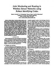
Fig. 1 Scenario Layout

Figure 1 depicts the scenario we studied in the work reported here. The simulated area has a size of 10 km x 10 km. The node in the lower right corner which is labeled “sink 0” is the base station, the 20 small nodes are the deployed sensor nodes. As it can be seen, the fire breakout is exactly at the center of the area. In the simulation, we consider that the forest fire breaks out 30 seconds after the simulation start. To avoid an unrealistic, circular spread of the fire, but still keeping the scenario simple, an elliptical spread is assumed with a spreading speed of


7

1 m/s on the minor axis and 2 m/s on major axis of the ellipse. The ellipse’s angle (in radians) with respect to the coordinate system is 0.5. The red shape visualizes the ellipse’s angle and the ratio between the major and minor axes. When the expanding fire ellipse reaches a node, its temperature increases rapidly. The maximum temperature a node can withstand is set to 130 degrees Celsius, when the value is above this threshold, the node dies (which means it is completely deactivated in the simulation). The nodes measure the temperature every 15 seconds and transmit the obtained values to the base station as input into a forest fire detection algorithm and fire fighter alerting. We have modelled an individual starting time for a nodes’ first measurement to avoid effects caused by synchronous transmissions of all nodes. As the temperature might not be the only data that a node is sending, the measured values are part of a data packet of 1 kBit size. This means each node is transmitting 1 kBit every 15 seconds, resulting in an overall rate of generated data at all nodes of 1.33 kBit/s or 1.33 packets/s. The transmission power, which is equal for all nodes in the scenario, is chosen so that multiple hops are required to reach the sink. Only the four nodes that are closest to the sink are in direct communication range with it.

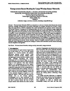
5 Computer Simulation The simulations for the evaluation of the proposed routing method were performed using the network simulator OPNET [3] with the simulation layout described in the previous section of this paper. The MAC (Medium Access Control) and PHY (Physical) layers in the node model are based on the Open-ZB [2] implementation (version 1.0) of the 802.15.4 stack. Different from the original Open-ZB model, the MAC layer was modified to support an ad-hoc mode with unslotted CSMA/CA instead of the original PAN-coordinated mode. We simulated the scenario for one hour in order to reach a statistical equilibrium. Several statistics were collected and are shown in the following. For comparison, the same scenario was simulated using AODV (Ad-hoc On-demand Distance Vector) [1] as the routing method. Here, the existing AODV implementation of OPNET’s wireless module was used and the PHY and MAC layers were replaced with the 802.15.4 layers. Figure 2 shows the temperature at sensor node 1, a node that is located close to the fire breakout location. It can be clearly seen that the temperature, which initially varies around a constant value (20 degrees Celsius) increases quickly when the fire reaches the node. Within a short time, the maximum temperature threshold is reached and the node dies. This temperature graph is shown to illustrate the conditions the nodes experience when the fire reaches them. Real temperature curves might have a smoother nature, which would make it even easier for a health-aware routing protocol to adapt to the changing conditions.

8


o

Temperature ( C)

150

100

50

0

0

500

1000

1500 2000 Model time (s)

2500

3000

3500

Fig. 2 Temperature at sensor node 1

Sensor ID

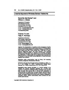
Figure 3 shows the packet reception statistics from the individual sources (sensor nodes) at the sink. The values on the ordinate are the IDs of the sensor nodes. Each blue cross marks the reception of an individual packet from the respective source at the sink. A continuous incoming flow of data from each node is visible (although the interarrival times vary in some cases). The flow of data stops abruptly when the node dies.

19 18 17 16 15 14 13 12 11 10 9 8 7 6 5 4 3 2 1 0 0

500

1000


2500

3000

3500

Fig. 3 Incoming packet flows at the sink

The death of nodes leads to less data traffic being generated and being received at the sink. This can be seen in the packet generation and reception rates shown


9

in Figure 4. The blue curve shows the generation rate, the red curve shows the reception rate. It has to be noted that both curves show moving average values in a 250 s time window, so that the curves are smoother and the difference between generation and reception is more visible. For comparison, the packet generation and reception rates were also measured in the AODV simulation and are shown in 5.

1.4 generated traffic received traffic 1.2

Traffic (packets/s)

1 0.8

0.6 0.4

0.2

0 0

1000

2000


5000

6000

Fig. 4 Traffic generated and received at the sink in packets/s (EMA routing)

One more performance measure that was recorded in the simulations was the end-to-end delays. These were not recorded for each source node separately, but across all source nodes. The results for both routing methods can be seen in Figure 6 with the crosses marking the AODV end-to-end delays and the dots marking the delays for EMA. Each cross or dot represents the reception of an individual packet.

6 Discussion The EMA algorithm performs as intended - as can be seen in Figure 3 - as the traffic of all sensor nodes reaches the sink, and the inflow of data packets continues until sensor nodes die. As Figure 3 does not directly show how much of the generated traffic is received at the sink, the incoming packet rate is compared to the generation rate in Figure 4. From this chart, it can be seen that until around 3500 seconds of model time have passed, the incoming packet rate is on the level of the generated rate, which is 1.33 packets/s when all nodes are alive (see section 4). The steep drop that follows is caused by the failure of sensor node 17. When this node fails, the

10


1.4 generated traffic received traffic 1.2

Traffic (packets/s)

1 0.8

0.6 0.4

0.2

0 0

1000

2000


5000

6000

Fig. 5 Traffic generated and received at the sink in packets/s (AODV routing)

0.2 AODV EMA

0.18

End−to end delay (s)

0.16 0.14 0.12 0.1 0.08 0.06 0.04 0.02 0 0

1000


4000

5000

Fig. 6 End-to-end delays in seconds

nodes in the upper right area can not reach the sink any more. The second significant drop is the failure of sensor node 5, after which no node can reach the sink any more (sensor node 0, which is also close to the sink, has already failed before). The result shows that the protocol succeeds in changing the routing in time before


11

transmission problems occur. The AODV results shown in Figure 5 show a lower and varying incoming packet rate throughout the simulation. This means there are less successful transmissions in the AODV scenario. This was observed for various settings of AODV parameters such as allowed hello loss, hello intervals, route request TTL settings and so on. The end-to-end delays, depicted in Figure 6, show that the proposed EMA algorithm in average is also providing slightly lower delays. While the delays are mostly between 20 and 30 ms in the AODV results, the delay results of the new algorithm proposed in this paper often are some ms lower, with a significant portion of them below 20 ms. The comparisons show clearly that the proposed EMA routing approach is superior to the quite common AODV routing protocol in the given scenario. However, further investigations have to be made though, to prove that these results also hold in different scenarios, and comparison has to be made to other sensor network routing methods, too.

7 Conclusion and Outlook We have proposed a routing approach that proactively adapts routes in a wireless sensor network based on information on node-threatening environment influences. The approach, called EMA routing, has been evaluated by computer simulation and has shown good performance in the considered forest fire scenario. With respect to the considered network and performance parameters, it outperforms the well known AODV routing algorithm. Further research will include evaluation in further scenarios, not only scenarios with a single-sink but also multiple-sink scenarios. Based on the neighbor selection/ route evaluation function, the specific routing scenario will be generalized into an approach for context-aware routing in sensor networks, where the evaluation function is not static, but can be modified according to changes in the context. Acknowledgements Parts of this work were performed under the framework of the Network of Excellence on Sensor Networks CRUISE partly funded by the European Commission in the 6th Framework IST Programme.

References 1. C. Perkins, E. Belding-Royer, S. Das, Ad hoc On-Demand Distance Vector (AODV) Routing, IETF RFC 3561, July 2003. 2. Open-ZB, OpenSource Toolset for IEEE 802.15.4 and ZigBee, http://open-zb.net, 2007. 3. OPNET, OPNET Modeler, http://opnet.com/solutions/network rd/modeler.html, 2007.

12


4. W.B. Heinzelman, A.P. Chandrakasan, H. Balakrishnan, An application-specific protocol architecture for wireless microsensor networks, IEEE Transactions on Wireless Communications , 1(4): 660-670, October 2002. 5. S. Lindsey, C.S. Raghavendra, PEGASIS: power efficient gathering in sensor information systems, in: Proc. IEEE Aerospace Conference, Big Sky, Montana, March 2002. 6. A. Manjeshwar and D.P. Agrawal, TEEN: A Protocol For Enhanced Eficiency in Wireless Sensor Networks, in Proceedings of the 1International Workshop on Parallel and Distributed Computing Issues in Wireless Networks and Mobile Computing, San Francisco, CA April 2001. 7. J. Kulik, W. Heinzelman, H. Balakrishnan, Negotiation based protocols for disseminating information in wireless sensor networks, ACM Wireless Networks, Vol. 8, Mar-May 2002, pp.169-185. 8. D. Intanagonwiwat, R. Govindan, D. Estrin, J. Heidemann, F. Silva, Directed diffusion for wireless sensor networking, IEEE/ACM Transactions on NetworkingIEEE/ACM Transactions on Networking, 11, February 2003. 9. C. Pandana, K.J.R. Liu, Maximum connectivity and maximum lifetime energy-aware routing for wireless sensor networks, in Proc. of Global Telecommunications Conference GLOBECOM 2005. 10. K. Kalpakis, K. Dasgupta, P. Namjoshi, Maximum Lifetime Data Gathering and Aggregation in Wireless Sensor Networks, in Proc. of the 2002 IEEE International Conference on Networking (ICN’02), Atlanta, Georgia, August 26-29, 2002. 11. C. Mascolo, M. Musolesi, SCAR: Context-Aware Adaptive Routing in Delay Tolerant Mobile Sensor Networks, in Proc. of the 2006 International Conference on Wireless Communications and Mobile Computing, 2006, pp. 533-538. 12. M. Musolesi, S. Hailes, C. Mascolo, Adaptive Routing for Intermittently Connected Mobile Ad Hoc Networks, in Proc. of the Sixth IEEE International Symposium on a World of Wireless Mobile and Multimedia Networks (WoWMoM) 2005, pp. 183-189. 13. Q. Liang, Q. Ren, Energy and Mobility Aware Geographical Multipath Routing for Wireless Sensor Networks, in Proc. of the IEEE Wireless Communications and Networking Conference 2005, pp. 1867-1871.