Measurement Techniques, Vol. 50, No. 8, 2007
ESTIMATING THE EFFECTS OF ADC PARAMETERS ON THE STATISTICAL CHARACTERISTICS OF THE SIGNAL FROM A SIMULATED OPTOELECTRONIC SYSTEM
V. I. Alekhnovich, A. S. Martynov, A. V. Perchik, and G. I. Utkin
UDC 519.8:681.7.01
An effective model is proposed for evaluating the effects of analog-to-digital converter (ADC) errors on the value distribution in the output sequence for any distribution of the input, together with a method of estimating ADC performance for statistical studies on signals. Key words: distribution, ADC, differential nonlinearity.
Much importance attaches to research on the statistical parameters of optical signals, which provides evaluation of the noise characteristics of sources and receivers, as well as components of the electronic system, and thus to construct probabilistic models. Current developments in digital engineering allow one to simplify and accelerate signal processing; digital computing is used in simulating optoelectronic systems in order to accumulate large volumes of data and perform analyses of any complexity. In digital processing, the analog electrical signal from the optical radiation detector is transformed by an analog-todigital converter (ADC) into a random digital sequence. The number distribution in it is influenced by the distribution in the input signal and by the errors of the electronic system and ADC. The analysis may include for example a comparison of the numbers of 0 and 1 in the bit representation of the sequence or comparison of the distribution with a given law [1]. An exact model for conversion of an analog signal into a series of digital values [2] is quite complicated even when one neglects the nonideal behavior in a converter. For statistical studies, the most important characteristics are those of converters obtained on large samples of the input signal. Here we consider an effective model that describes the distributions of the random input signal and discrete random sequence at the output and which enables one to estimate the effects of the converter error on the distribution in the output sequence no matter what the input distribution. That model is used in a method of evaluating ADC performance for statistical signal studies. Consider the conversion of a random signal by a converter working with M bits and having N = 2M combinations at the output. The voltage scale is conveniently considered in relative values u = U/Ufs, where Ufs is the full-scale voltage (subject to the condition that the lower boundary of the dynamic range for the ADC is 0). Let the input signal u = u(t) be characterized completely by the probability pu(u) and probability function Pu(u) as defined in [3]: u
Pu (u) = P{ν < u} =
∫ pu ( ν)dν ,
−∞
i.e., the probability of the voltage falling at the input in the range from –∞ to u. State Research Center of Scientific Instrumentation at Bauman Moscow State Technical University; e-mail:
[email protected]. Translated from Izmeritel’naya Tekhnika, No. 8, pp. 12–15, August, 2007. Original article submitted March 27, 2007. 0543-1972/07/5008-0817 ©2007 Springer Science+Business Media, Inc.
817
For combination i to occur (i = [0 ... N – 1]), the input voltage should fall in the range [ui; ui+1], where ui and ui+1 are the lower and upper bounds to the voltages in range i. The probability of this happening is defined [3] as the difference of the probabilities of occurrence at the input of voltages in the ranges (–∞; ui+1] and (–∞; ui): Pu,i = Pu(ui+1) – Pu(ui).
(1)
If the input voltage exceeds the dynamic range of the converter, all values exceeding the limit will be transformed into limiting values of the digital codes (for example, for an eight-bit ADC these values are 0 and 255). This case is incorporated as follows: Pu,0 = Pu(u1) – Pu(–∞) = Pu(u1); Pu,N–1 = Pu(+∞) – Pu(uN–1),
(2)
where Pu(–∞) is the probability of there being a voltage less than infinitely large negative (or the probability of an impossible event); Pu(+∞) is the probability of occurrence of a voltage less than the infinitely large positive limit (or the probability of a reliable event). Then Pu,0 reflects the probability of the occurrence of a voltage less than the upper bound to the first range, while Pu,N–1 reflects the probability of the occurrence of a voltage above the lower bound of the last range. We consider the conversion on two types of random signals: with uniform or normal distributions. We write the probability densities for them as follows: • for a signal with uniform distribution
pu (u) =
1 u−u , u − u≤ 0.5 ; 1 rect = ub − u a ub − u a ub − u a 0 , u − u > 0.5 ,
• for a signal with normal distribution pu (u) =
(u − u )2 exp − , 2σ u 2 πσu 1
where ua and ub are the lower and upper bounds to the voltage range, u is the mean value of the voltage (signal), and σu is the standard deviation (SD). For simplicity, we consider an ADC with eight bits (256 values). If for it we use (1) and (2) to calculate the frequencies of occurrence of numbers at the output for these two types of random signals and block them as graphs, it becomes clear that the probability density of the analog random signal is the envelope of the distribution for the digital random sequence. This digital random signal may then be used in digital processing; an example is where one calculates the numbers of occurrences of 0 and 1 in the bits at the ADC output. That is useful in estimating the randomness of the distribution. The probabilities of 0 or 1 occurring in the least-significant bit are given by 127
P0 =
∑ Pu ,2 k ;
(3)
k =0 127
P1 =
∑ Pu ,2 k +1 ,
k =0
in which P0 and P1 are the probabilities of occurrence in the least-significant bit of values of 0 and 1, respectively. 818
(4)
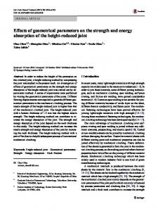
a
b
Fig. 1. Occurrence frequencies for numbers at the ADC output for input signals with displaced mean values: a) uniform distribution; b) normal distributions; 1) σu = 0.5/6 = 0.083, 2) σu = 0.5/3 = 0.167.
TABLE 1. Occurrence Frequencies for 0 and 1 in the Bits of the Numerical Sequence Occurrence frequencies for numbers Input signal distribution 0
1
0.495836
0.504164
with low dispersion
0.499993
0.500007
with high dispersion
0.490835
0.509165
Uniform Normal
For these types of signals, these probabilities are P0 = P1 = 0.5. The same principle can be used in models for other transformations, including more complicated ones. The (1) correction allows one to incorporate the correction to the output signal due to mismatch between the signal voltages at the ADC input and the working voltage range. Consider the case where the mean value of the input random analog signal is displaced with respect to the center of the dynamic range, with the other parameters unaltered. Figure 1 shows the frequencies of occurrence in the random sequence at the ADC output, while Table 1 gives the frequencies of 0 and 1 in the bits as calculated from (3). The values of the frequencies on the graphs have been calculated for distributions as follows in the random signal at the ADC input: uniform with ua = 0, ub = 1, u = 0.5, normal with u = 0.5 and low SD σu = 0.5/6 = = 0.083 (curve 1) and the same with large SD σu = 0.5/3 = 0.167 (curve 2). The graphs show that the transformation shifts the histogram in the same direction as the initial-signal density distribution, where voltages exceeding the boundary of the normal range are converted into extreme digital values (maximal or minimal). This distorts the distribution after transformation, which is evident from the inequality of the frequencies of 0 and 1 in the sequence. If the distribution is uniform or normal with height dispersion, then even slight displacement of the mean value causes marked distortion in the output distribution. The displacement is not critical for a signal with normal distribution and small dispersion. In an ideal ADC, the quantization step is constant, and the boundaries to range i are readily determined as ui = ih – lower, ui+1 = (i + 1)h – upper.
(5)
The quantization step is not constant in a real converter. The difference between the transformation quantum hi and the mean value h is called the differential nonlinearity of the ADC conversion characteristic. In the specifications for 819
a
b
Fig. 2. Frequencies of occurrence of numbers in the output sequences of an ideal ADC: a) uniform distribution; b) normal distributions with 1) σu = 0.5/6 = 0.083, 2) σu = 0.5/3 = 0.167.
TABLE 2. Occurrence Frequencies for 0 and 1 in the Bits in the Sequence at the Output from a Nonideal ADC Number occurrence frequencies Input signal distribution
Uniform
0
1
0.498016
0.501984
Normal: with low dispersion
0.493025
0.506975
with high dispersion
0.492610
0.507390
particular converters, the differential nonlinearity is expressed in fractions of the least-significant bit or the percentage of the full scale [4]. We now consider the effects of the differential ADC nonlinearity on the statistical characteristics of the random output sequence. To determine the upper and lower bounds for the interval for value i, we need to know the quantization steps for all the preceding values: i =1
ui =
∑ hk
k =0
i
– lower, u0 = 0, ui +1 =
∑ hk
– upper.
(6)
k =0
These bounds can be used in (2) to calculate the probabilities of the signal forming in the given interval. It is difficult to use (1) because one lacks exact values for the quantization steps. This can be simplified on the following assumption: the differential characteristic error affects only the quantization step, not the middle of the range. This can be assumed because the makers of ADC tend to set the centers of the intervals on a single straight line. We can say that by comparison with an ideal ADC, some intervals contain more voltage values and others fewer. To incorporate these changes, we can introduce the relative probability δPi, which indicates by what factor the given value of i is more probable than when one uses an ideal converter, and which is calculated as δPi = hi /h,
(7)
in which hi is the quantization step for value i in the real ADC and h is the quantization step for an ideal ADC with the same number of bits. 820
The random-signal conversion may thus be divided into two parts: ideal, working as an ideal ADC in accordance with (1), and correcting. The probabilities of occurrence at the ADC output of the numbers i are calculated as the products of the probabilities of occurrence of that number at the output of an ideal ADC and the relative probabilities: Pi = PiidδPi,
(8)
in which Piid is the probability of occurrence of i at the output of an ideal ADC as calculated from (1) with the bounds of (5). The error calculated from (8) differs from the calculation on (1) with the bounds of (6) by not more than 0.01%. Consider a nonideal eight-bit ADC in which the quantization steps for the values 96 and 156 are less by factors of 2 than for an ideal one. The quantization steps for all the other values are correspondingly increased: 0.5 , i = 96 , i = 156 ; δPi = 1 = 1.00390625 , i ≠ 96 , i ≠ 156 . 1 + 256
(9)
From (1) we determine the distribution at the output of the ideal eight-bit ADC. Figure 2 shows the histogram for the distribution of the output from a nonideal ADC on the basis of (8) and (9). Figure 2 implies that the probabilities of occurrence for the numbers 96 and 156 at the ADC output are also less by factors of 2 than for the ideal case. Such probability changes may lead to changes in the output signal characteristics after additional processing. For example, from (3) and (4) one can determine the distribution of the numbers obtained with the least-significant ADC bit. The table shows the deviations from equality in the frequencies of occurrence of 0 and 1 in the bits of the output sequence. These models may be used to set up methods for the statistical evaluation of ADC and digital systems. The random input is specified as the probability density on the basis of the relative voltage. Then from (1) and (2) we determine the probabilities of number occurrence at the output of an ideal ADC. The nonideal behavior is corrected for by means of the probabilities of (9). If necessary, one can apply statistical models for the subsequent transformations. It is convenient to use the method based on relative probabilities of (7) in that the actual characteristics of the ADC can be determined by experiment. An input random signal with uniform distribution over the range 0 ≤ u ≤ 1 gives the probability of occurrence of the value i determined by (1) with (2): Pu ,i = Pu (ui +1) − P(ui ) =
ui +1
ui
−∞
−∞
∫ p( ν)dν − ∫ p( ν)dν =
ui ui +1 = pu p( ν) dν − p( ν) dν = pu (ui +1 − ui ) , −∞ −∞
∫
∫
1 = pu = 1 = const is the value of the input signal probability density. 1− 0 The relative probability can be determined as the ratio of the probabilities for the occurrence of the number i at the outputs of ideal and nonideal ADC:
where pu (u) =
id δPi = Piid/Pi = pu(u id i+1 – ui )/pu(ui+1 – ui) = hi /h.
Here Piid is calculated theoretically from the number of ADC bits, while Pi is found as the occurrence frequency for number i in a sequence at the test ADC output with a large sample volume: Pi = Ni /N, where Ni is the number of occurrences of i in the sample; N is the sample volume, N → ∞. 821
The main difficulty lies in producing an analog signal with a uniform distribution. One can use a sawtooth generator or a high-precision DAC [4]. This method has been used in software for fast experimental estimation of ADC performance not only for an individual realization, but also for averaging over a set of realizations. These data can be used in simulating a hybrid optoelectronic system by the use of statistical models.
REFERENCES 1. 2. 3. 4.
822
V. I. Alekhnovich et al., Izmer. Tekh., No. 11, 33 (2006); Measurement Techniques, 49, No. 11, 1114 (2006). E. I. Tsvetkov, The Principles of Mathematical Metrology [in Russian], Politekhnika, St. Petersburg (2005). E. S. Venttsel’ and L. A. Ovcharenko, Probability Theory and Its Engineering Applications [in Russian], Vysshaya Shkola, Moscow (2000). T. S. Rakhtor, Digital Measurements: ADC/DAC [in Russian], Tekhnosfera, Moscow (2006).