AbstractâIn this paper, we consider the decentralized es- timation over non-orthogonal multiple-access fading channels. (MACs) with zero-mean channel ...
This full text paper was peer reviewed at the direction of IEEE Communications Society subject matter experts for publication in the IEEE Globecom 2010 proceedings.
Estimation Feedback and Bandwidth Allocation with the Type-based Multiple-access in Wireless Sensor Networks Xin Wang and Chenyang Yang School of Electronics and Information Engineering Beihang University, Beijing, China, 100191
Abstract—In this paper, we consider the decentralized estimation over non-orthogonal multiple-access fading channels (MACs) with zero-mean channel coefficients in wireless sensor networks (WSNs). Using the type-based multiple-access (TBMA) with bandwidth extension transmission scheme, we introduce a low-complexity two-stage estimator and analyze its performance. It shows that the performance can be improved by allocating bandwidth among types, but the optimal bandwidth allocation scheme requires a priori information of the parameter being observed. We then introduce a broadcasting feedback method for the sensors to obtain the required information. This feedback scheme is more efficient and feasible than the channel state information (CSI) feedback over orthogonal MACs. Besides the estimation accuracy, we also evaluate the bandwidth efficiency of the proposed methods by introducing a metric as the bandwidth normalized performance gain in simulations. It shows that the proposed feedback and bandwidth allocation schemes outperform the TBMA with CSI feedback in non-orthogonal MACs and the optimal transmission scheme in orthogonal MACs at typical operating signal-to-noise ratio levels of the WSNs.
I. I NTRODUCTION One of the main functions of wireless sensor networks (WSNs) is sensing physical phenomena. For the decentralized estimation, typical WSNs usually consist of many wireless sensors spatially scattered in a field to observe some parameters of interest, then convert their observations into waveforms. These waveforms are transmitted to the fusion center (FC) over multiple-access channels (MACs), and the FC will generate the estimation of the parameters being observed. Decentralized estimation over orthogonal MACs has been studied in [1] and references therein. However, because the scale of the WSNs is usually larger than that of the traditional wireless networks [2], orthogonal multiple-access protocols are hard to implement and their bandwidth efficiency will decrease with the increasing of the network scale. Therefore, the transmission over non-orthogonal MACs, which is usually more bandwidth efficient, has received considerable attention recently both in decentralized estimation [3]–[6] and detection [7]–[10]. Several transmission schemes have been proposed for the decentralized estimation in nonorthogonal MACs, including the analog amplify-and-forward [11]–[13], the type-based multiple-access (TBMA) [3], [14], This research was supported by the National Natural Science Foundation of China (NSFC) under Grant 60672103.
[15], the analog constant modulus modulations [16], and the likelihood-based multiple-access [5], etc. These schemes make it possible for the FC to recover the sufficient statistics from the received signals, then estimate the parameter [6]. It is shown in [3], [17] that the asymptotic performance of these sufficient statistics based transmission schemes are superior to that of the orthogonal multiple-access transmission schemes in both error-free and AWGN channels. In fading channels with non-zero mean, the estimation using these schemes is still asymptotic efficient [3] with some performance sacrifices. But the performance of these methods decreases dramatically in zero-mean fading MACs. Some methods have been introduced to improve the estimation performance in zero-mean fading channels, e.g., the channel state information (CSI) feedback from the FC to the sensors then the phase compensation at the sensors [14], [15], [18]. However, when implementing the CSI feedback, it still needs the orthogonal multiple-access protocols for the sensors to transmit training sequences and for the FC to feed the estimated CSI back to each sensor, which also leads to low efficiency. We introduce the TBMA with bandwidth extension (TBMABE) transmission scheme and a corresponding approximate maximum likelihood (ML) estimator in [19], which requires no feedback from the FC but uses more bandwidth resources. In this paper, we consider the decentralized estimation over non-orthogonal multiple-access fading channels with zero-mean channel coefficients. The TBMA-BE transmission scheme is considered and a corresponding low complexity two-stage estimator is introduced with the proposed transmission scheme. During the first stage, the estimator uses the ML estimation to estimate the empirical measurement [20] from the received signals. While during the second stage, it uses an optimal fusion to estimate the parameter by minimizing the Kullback-Leibler distance between the estimated empirical measurement and the actual probability mass function (PMF) which contains unknown parameter. The analysis of this two-stage estimator shows the optimal bandwidth allocation method among the types, which needs a priori information of the parameter being observed at the sensors. To make this information available at the sensors, we introduce a practical feedback method. This method only requires broadcast feedback channel from the FC to the
978-1-4244-5638-3/10/$26.00 ©2010 IEEE
This full text paper was peer reviewed at the direction of IEEE Communications Society subject matter experts for publication in the IEEE Globecom 2010 proceedings.
sensors. We show that it improves the estimation accuracy, and its energy and bandwidth efficiency are superior to that of reference schemes at low communication signal-to-noise ratio (SNR) levels, which are typical operating points of the WSNs. The bandwidth allocation and feedback methods further improve the estimation accuracy and bandwidth efficiency of the TBMA-BE transmission scheme compared with the uniform bandwidth allocation considered in [19]. The rest of the paper is organized as follows. Section II describes system models. Section III introduces the twostage estimator and analyzes its performance, then presents the bandwidth allocation and feedback methods. Simulation results are provided in Section IV and the conclusions are given in Section V.
TBMA-BE transmission scheme, where m = 1, · · · , M, k = 1, · · · , Km , and Ts is the duration of the waveforms. To simplify the analysis, the energy of φm,k (t) is normalized to one. When the i-th sensor observes the mi -th type and selects ki -th waveform to transmit, the transmitted signal of it is si (t) =
K M � � � Ed Ei (m, k)φm,k (t),
(2)
m=1 k=1
where Ed is the energy used by each sensor to transmit one observation, and Ei (m, k) is defined as � 1, m = mi , k = ki . (3) Ei (m, k) = 0, otherwise C. Received Signal
II. S YSTEM M ODELS A. Observations and Quantizations We consider the observation model as in [3], [18], [21], where N sensors observe a deterministic scalar parameter θ. The sensors transmit their signals to the FC directly and there are no inter-sensor communications. The observation provided by the i-th sensor is xi = θ + ns,i , i = 1, · · · , N,
(1)
We assume that the channels are the block fading, i.e., the channel coefficients are invariant during the period that sensors transmit the signals representing one observation. We also consider the synchronous MACs as in [3], [18]. The received signal at the FC is then y(t) =
N �
hi si (t) + n(t), i = 1, · · · , N,
(4)
i=1
where ns,i is independent identically distributed (i.i.d.) observation noise, which subjects to the Gaussian distribution with zero mean and variance σs2 . We assume that θ is bounded with a dynamic range [−V, +V ]. After the observations, the sensors quantize their observations into M types for the type-based transmission [3]. We define mi as the index of the type corresponding to observation xi after the quantization. The uniform quantizer is used by the sensors because it is optimal for the deterministic parameter. Assume that the dynamic range of the quantizer, [−W, +W ], is much larger than the dynamic range of θ, thus the probability that xi is out of [−W, +W ] can be ignored.
where hi is the channel coefficient, which subjects to complex Gaussian distribution with zero mean and unit variance, i.e., hi ∼ CN (0, 1), and n(t) ∼ CN (0, σc2 ) is the thermal noise of the receiver.
B. Transmission Scheme
where nm,k is i.i.d. complex Gaussian noise with zero mean and variance σc2 , and �x(t), y(t)� is the inner product of x(t) and y(t). For convenience, we define the following vectors, • ym = [ym,1 , · · · , ym,Km ], T T T • y = [y1 , · · · , yM ] . The optimal ML estimator for estimating θ directly has high computational complexity [19]. Therefore, we introduce a low complexity estimator with two stages. During the first stage, we use the ML criterion to estimate the empirical measurement [20]. During the second stage, we derive an optimal estimator of θ based on the estimation of the first stage. Both the estimators in these two stages have closed forms, which consist only simple computations, thus the complexity is much reduced compared with the ML estimator shown in [19]. Define p(m, k|θ) as the PMF that a sensor observes the m-th type and selects k-th waveform, and Nm,k is the actual number of the sensors observes the same type and selects the same waveform. The empirical measurement of p(m, k|θ) is
The transmission scheme considered is the TBMA-BE as shown in [19], which makes it possible to allocate the bandwidth resources among the types. By this transmission scheme, the m-th type is represented by Km orthogonal waveforms and the sensors randomly select one among Km waveforms to transmit. When Km = 1, ∀m = 1, · · · , M , the TBMA-BE degenerates into the TBMA transmission. Note that in [7] where the distributed detection using TBMA transmission scheme is considered, an optimal transmission rate is introduced to control the number of the active sensors in a time slot to improve the performance of the detection over zero-mean fading channels. The sensors transmit the signals randomly in different time slots, which can be regarded as transmission using different orthogonal waveforms. But [7] does not consider the bandwidth allocation between two hypotheses, say, two types, of the detection problems. Now we introduce the transmitted signal model. Define φm,k (t), 0 ≤ t ≤ Ts , as the orthogonal waveforms used by
III. E STIMATION , F EEDBACK AND BANDWIDTH A LLOCATION After using the waveform matched filter, the discrete received signal at the FC becomes, ym,k = �y(t), φm,k (t)� =
N � � Ed hi Ei (m, k) + nm,k , (5) i=1
978-1-4244-5638-3/10/$26.00 ©2010 IEEE
This full text paper was peer reviewed at the direction of IEEE Communications Society subject matter experts for publication in the IEEE Globecom 2010 proceedings.
defined as pm,k = Nm,k /N . Also for convenience, we define the vectors, • pm = [pm,1 , · · · , pm,Km ], T T T • p = [p1 , · · · , pM ] . Similarly, we can define the p(m|θ) as the PMF that a sensor observes the m-th type�and its empirical measurement pm = Km Nm,k . Nm /N , where Nm = k=1 Note that [3] also introduces a two-stage estimator based on the empirical measurement in the AWGN and nonzero-mean fading MACs. In AWGN MACs, the received signal is y = p + n, where n is a vector consisting i.i.d. Gaussian noises. It is not hard to show that y itself is the optimal estimate of p. In fading MACs with nonzero-mean channel coefficients, y is still an estimate of p with performance loss. However, when the channel coefficients are zero mean, y itself is no longer an estimation of p. A. ML Estimator of the Empirical Measure We use the ML estimation to estimate p during the first stage. Given p, the received signal vector y is complex Gaussian distributed based on the received signal model. The log-likelihood function for estimating p is then, log p(y|p) = −
After deriving the probability distribution function of pˆnc m,k and computing its mean and variance, it shows that pˆnc m,k is an unbiased estimate of pm,k with variance (Ed N pm,k + σc2 )2 1 2pm,k = p2m,k + 2 2 + , 2 2 Ed N N γc N γc (9) where γc = Ed /σc2 is the communication SNR. Since pˆnc m,k are independent with each other, the variance of nc pˆm is the summation of the variance of pˆnc m,k as Var[ˆ pnc m,k ] =
Var[ˆ pnc m]
=
Km � k=1
Km �
min
pm,k
k=1 Km �
log(Ed N pm,k + σc2 )+
|ym,k |2 Ed N pm,k + σc2
s.t.
� + α,
(6)
where α is a constant with no influence on the estimation. We first find the maximum of the log-likelihood function without introducing any constraint on pm,k . By computing the first and second order derivatives of (6), it shows that the loglikelihood function has only one maximum, which is achieved when |ym,k |2 − σc2 , (7) pˆnc m,k = Ed N where pˆnc m,k is named as the unconstrained ML estimator of p. Because pm,k represents a probability, there should be a non-negative constraint, which is pm,k ≥ 0, and a summation �M �Km constraint, which is m=1 k=1 pm,k = 1, on it. However, pˆnc shown in (7) does not always satisfy these m,k constraints. Because the likelihood function is non-concave, we can only solve the ML problem with the non-negative constraint by omitting the summation constraint. We can show that the non-negative constraint ML estimator is + pnc pˆcm,k = (ˆ m,k ) ,
(8)
where the operator (x)+ = max(0, x). Following the invariance property of the ML estimator, we can obtain that the unconstrained ML estimator and the non-negative constrained ML estimator of pm are pˆnc m = � � Km nc K m c c p ˆ and p ˆ = p ˆ , respectively. m k=1 m,k k=1 m,k Now we analyze the estimation performance of the first stage estimators. For mathematical tractability, we use pˆnc m,k to analyze.
Km 2pm + . N 2 γc2 N γc
(10)
It is shown in (10) that the variance depends on pm,k . Although pm,k is a stochastic variable, we can still design its distribution to minimize the variance of pˆnc m . In the sequel, we first find an optimal pm,k to minimize (10), then design p(m|θ) according to the characteristic of the optimal pm,k . Ignoring the unrelated terms, the optimization problem to find optimal pm,k is
Km M � � � m=1 k=1
p2m,k +
p2m,k pm,k = pm .
(11)
k=1
Using the method of Lagrange multiplier, the minimum of the objective function in (11) can be obtained as �Km Km � pm,k )2 ( k=1 p2 p2m,k ≥ = m, (12) Km Km k=1
which is achieved when pm,k = pm /Km for all k. The optimal pm,k suggests that the signals from the sensors should be uniformly distributed on Km orthogonal dimensions. Therefore, we let the sensors to select the waveform with equal probability, which means that the PMF p(m, k|θ) = p(m|θ)/Km . When pm,k = pm /Km , (10) becomes, Var[ˆ pnc m] ≥
p2m Km 2pm + 2 2+ . Km N γc N γc
(13)
It is not a monotonic function with respect to Km . Computing its derivative, its minimum is Var[ˆ pnc m] ≥
4pm , N γc
(14)
which is achieved when ∗ Km = N γ c pm .
(15)
It is shown in (15) that the optimal Km is proportional to the number of the sensors and the communication SNR. When Km is large, there are more waveforms for the sensors to select, thus the signals from different sensors will be distributed on different waveforms with large probability. Therefore, the first term in the right hand side of (13) will become small.
978-1-4244-5638-3/10/$26.00 ©2010 IEEE
This full text paper was peer reviewed at the direction of IEEE Communications Society subject matter experts for publication in the IEEE Globecom 2010 proceedings.
However, the larger bandwidth will introduce more noise, which deduces the estimation accuracy. Hence the optimal Km is the trade-off between these two conflicting factors. When the communication SNR is low or the number of the sensors is small, little orthogonal dimensions should be used in order to gather the energy of the transmitted signals for combating the noise. On the contrary, when the communication SNR is high or the number of the sensors is large, the transmitted signals should be scattered to more orthogonal dimensions. We can use (15) to design the bandwidth allocation scheme among the types, which will be introduced in Section III-C. B. Optimal Estimator of the Parameter Being Observed ˆcm,k are the estimators of the probability Both pˆnc m,k and p that the sensor observes the m-th type and selects k-th type given θ, i.e., p(m, k|θ). In the rest of the paper, we consider that the sensors select the waveform with equal probability, thus p(m, k|θ) = p(m|θ)/Km . Since the relative entropy, also referred to as KullbackLeibler distance [22], can be regarded as the distance between two distributions, we design an estimator of θ to minimize the relative entropy. Because pˆnc m,k may be negative, which makes no sense when computing the relative entropy, we use pˆcm,k to derive the estimator. Define ˆ = [pc1,1 , · · · , pcm,k , · · · , pcM,KM ]T p
(16)
as the estimation of p(m, k|θ) and pθ = [p(1, 1|θ), · · · , p(m, k|θ), · · · , p(M, KM |θ)]T
(17)
as the actual PMF that depends on the unknown parameter. The estimator of θ can be obtained by solving the following unconstrained optimization problem, � � Km M � � pˆcm,k . (18) p�pθ ) = pˆcm,k log min D(ˆ θ p(m|θ)/Km m=1 k=1
To derive the solution of the problem (18), we use the Lagrange’s Mean Theorem to approximate p(m|θ) as follows, � � (x − θ)2 1 √ p(m|θ) = dx exp − 2σs2 2πσs Im � � Δ (Sm − θ)2 ≈ √ , (19) exp − 2σs2 2πσs where Im is the quantization interval, which length is Δ, and Sm is the medium value of the quantization interval. For the considered observation model, both the exact and the approximate form of p(m|θ) are strictly greater than 0 for all θ and m, thus D(ˆ p||pθ ) always has minima, which is achieved when 1 θˆ = �M
M �
pˆcm Sm . c ˆm m=1 m=1 p
(20)
do not consider the constraint that �Kwe �Since M m c p ˆ = 1 during the first step, it can happen m=1 �M k=1c m,k that p ˆ = 0 when all pˆcm s equal to 0. In this case, m=1 m
(20) is undefined and the relative entropy D(ˆ p�pθ ) equals to zero for all θ. This case happens when the received energy of each orthogonal waveform is smaller than the variance of the thermal noise of the receiver, i.e., no signal but noise is received. It is hard to estimate the parameter no matter which estimator is used. However, there are several heuristic methods to obtain an estimate of θ. For example, we can let θˆ = Smmax , where mmax is mmax = argm max �ym �22 ,
(21)
where � · �2 is l2 -norm of the vector. C. Bandwidth Allocation and Feedback The variance of the estimator during the first stage is ∗ ∗ minimized by the optimal Km shown in (15), thus Km can be used to design the bandwidth allocation schemes. ∗ depends on pm , which is the value to be However, Km estimated during the first stage. Without this information, the sensors cannot compute the optimal bandwidth allocation scheme, and have to allocate the bandwidth uniformly to all types under the assumption that θ is uniformly distributed, which means that Km = K, ∀m. We name it as the uniform bandwidth allocation scheme. This scheme consume K times bandwidth resources compared with the TBMA where each type is represented by only one waveform. To make a priori information about pm available at the sensors, we consider a feedback scheme that the FC broadcasts its estimation of θ to the sensors, and the sensors use these information to obtain an estimation of pm by computing the PMF p(m|θ), then compute Km using pm = p(m|θ). Before the first feedback information is received, the sensors use the uniform bandwidth allocation. To highlight the feedback method, we assume that θ is invariant during the period of the feedback and new transmissions. When θ is a time sequence, the bandwidth allocation method can be extended with the statistical model of it. We also assume that the feedback is error-free since the FC is usually much more powerful than the sensors. Because the feedback value θˆ contains estimation error, Km ∗ computed using θˆ may severely mismatch Km , especially when the accuracy of θˆ is poor. To avoid this problem, we design a robust bandwidth allocation scheme introduced in the following. The estimation of θ can be represented as θˆ = θ+nθ , where nθ is the estimation error. We assume that nθ is Gaussian ˆ Both the mean ˆ and variance σ 2 (θ). distributed with mean b(θ) ˆ These two values and the variance are the function about θ. can be obtained off-line by simulations and stored in a table at the sensors. In our simulations, we quantize θˆ with the same ˆ and M -level quantizer used by the sensors, and obtain b(θ) ˆ for M possible quantization values of θˆ by simulations. σ 2 (θ) ˆ the conditional distribuAfter receiving the feedback of θ, tion of the parameter θ can be decided by the information provided from the feedback, which is
� ˆ + b(θ)) ˆ 2 (θ − θ 1 ˆ =√ exp − . (22) p(θ|θ) ˆ ˆ 2πσ(θ) 2σ 2 (θ)
978-1-4244-5638-3/10/$26.00 ©2010 IEEE
This full text paper was peer reviewed at the direction of IEEE Communications Society subject matter experts for publication in the IEEE Globecom 2010 proceedings.
The robust bandwidth allocation scheme is obtain as Km
= γc N Eθ|θˆ[p(m|θ)] +∞ ˆ p(m|θ)p(θ|θ)dθ. = γc N
(23)
−∞
We use the approximate PMF of p(m|θ) shown in (19) when computing the integration in (23), then we have the bandwidth allocation scheme as
� ˆ 2 (Sm − θˆ + b(θ)) Δ exp − . Km = γc N ˆ 2(σs2 + σ 2 (θ)) ˆ 2π(σs2 + σ 2 (θ)) (24) This feedback scheme is more efficient than the existing CSI feedback schemes [14], [15], [23], because it needs only broadcast channel and the feedback information is a single ˆ value θ.
normalized performance gain defined as Gmse , (25) G= Gbw where Gmse is the performance gain, which is the ratio between the MSE of TBMA and the that of the considered scheme, and Gbw is the bandwidth gain, which is the ratio between the bandwidth consumed by the considered scheme and that by the TBMA. When computing G, the bandwidth consumed by the partial CSI feedback is 3 bits per sensor because [18] shows that 3 bits feedback is enough, and the bandwidth consumed by the θˆ feedback is 8 bits, which is accurate enough and independent to the number of the sensors. M=16, N=10, γs=20dB −1
10
TBMA (K=1) TBMA−BE uniform K=2 TBMA−BE uniform K=3 TBMA CSI Feedback TBMA−BE BW Feedback Orth−MAC Opt
We will evaluate the mean square error (MSE) of estimating θ and the bandwidth efficiency using the TBMA-BE transmission scheme with the proposed estimation, bandwidth allocation, and feedback methods by simulations. The observation SNR is defined as γs = log10 (W 2 /σs2 ), and the communication SNR is defined as γc = log10 (Ed /σc2 ). In the simulations, we set the observation SNR as 20dB, and the number of the quantization levels M is 16 according to the results in [24]. We evaluate two kinds of bandwidth allocation schemes in the simulations. The first one is the uniformly allocation with different K denoted as “TBMA-BE uniform” in the legends. When K = 1, it becomes the TBMA transmission scheme denoted as “TBMA (K=1)”. The second one is the bandwidth allocation with proposed feedback method denoted as “TBMABE BW Feedback”. For comparison, we evaluate two schemes for reference in the simulations. The first one is the decentralized estimation over orthogonal MACs (“Orth-MAC Opt”). The curve is obtained under the assumption that the sensors use ideal multipleaccess protocols, i.e., the transmitted signals is orthogonal without multi-user interferences and the control frames used by the multiple-access protocols cost no bandwidth. The transmission codebook used in this simulation is the nearoptimal one shown in [25]. The bandwidth consumed by this transmission scheme is M × N . The second one is the TBMA with the partial CSI feedback shown in [18] (“TBMA CSI Feedback”). Only the phases of the channel coefficients are fed back to the sensors and the sensors compensate the channel phases before transmitting their signals, thus the signals arrive the FC coherently. Because the bandwidth consumption of the considered schemes is different, we take the TBMA transmission scheme as the benchmark to evaluate the bandwidth efficiency of the schemes. The bandwidth efficiency is evaluated by a
MSE
IV. S IMULATION R ESULTS −2
10
−3
10
4
6
Fig. 1.
8 10 Communication SNR/dB
12
14
MSE versus γc when N = 10.
Figure 1 plots the MSEs of the estimators as a function of the communication SNR γc . When the uniform bandwidth allocation is used, it shows that the performance depends on K. When γc is low, the transmission schemes with smaller K outperform that with larger K. On the contrary, the transmission schemes with larger K outperform that with smaller K when γc is high. At low communication SNR levels, the TBMA-BE scheme with feedback and bandwidth allocation outperforms the scheme in orthogonal MACs. While at high communication SNR levels, their performance is similar. The feedback and bandwidth allocation scheme is also superior to the TBMA with CSI feedback and compensation, even when the phase feedback is error-free. Figure 2 shows the bandwidth normalized performance gain of the transmission schemes as a function of the communication SNR. Even normalized by the bandwidth consumption, the TBMA-BE with the feedback and bandwidth allocation is more efficient than the other schemes at low communication SNR levels. Because the bandwidth allocation scheme requires the bandwidth to increase linearly with γc , its bandwidth efficiency decreases with γc . Since the low communication SNR levels are the typical operating points of the WSNs, the TBMA-BE with the feedback and bandwidth allocation is superior to the other schemes in practice.
978-1-4244-5638-3/10/$26.00 ©2010 IEEE
This full text paper was peer reviewed at the direction of IEEE Communications Society subject matter experts for publication in the IEEE Globecom 2010 proceedings.
M=16, N=10, γs=20dB 3 TBMA−BE BW Feedback TBMA CSI Feedback TBMA (K=1) TBMA−BE uniform K=2 TBMA−BE uniform K=3 Orth−MAC Opt
Bandwidth Normalized Gain
2.5
2
1.5
1
0.5
0
Fig. 2.
4
6
8 10 Communication SNR/dB
12
14
Normalized Performance Gain versus γc when N = 10.
V. C ONCLUSION We consider the decentralized estimation over nonorthogonal multiple-access fading channels with zero-mean channel coefficients. Differing from the existing CSI feedback schemes, we introduce the broadcasting feedback and bandwidth allocation schemes to improve the estimation performance. A two-stage low-complexity estimator is introduced with the TBMA-BE transmission scheme. By analyzing the performance of the estimation, we show that the optimal bandwidth allocation can improve the estimation accuracy, and the bandwidth allocation can be implemented with the broadcasting feedback information. The simulations show that the feedback and bandwidth allocation improve the estimation accuracy compared with the CSI feedback scheme. It is also shown that the proposed TBMA-BE with bandwidth allocation is superior to the transmission schemes in orthogonal MACs. Therefore, the proposed schemes are more efficient in both energy and bandwidth at typical operating SNR levels of the WSNs. R EFERENCES [1] J.-J. Xiao, A. Ribeiro, Z.-Q. Luo, and G. B. Giannakis, “Distributed compression-estimation using wireless sensor networks,” IEEE Signal Processing Magazine, vol. 23, no. 7, pp. 27–41, Jul. 2006. [2] I. F. Akyildiz, W. Su, Y. Sankarasubramaniam, and E. Cayirci, “Wireless sensor networks: A survey,” Computer Networks, vol. 38, no. 4, pp. 393– 422, Mar. 2002. [3] G. Mergen and L. Tong, “Type based estimation over multiaccess channels,” IEEE Transactions on Signal Processing, vol. 54, no. 2, pp. 613–626, Feb. 2006. [4] M. Gastpar, “To code or not to code,” Ph.D. dissertation, Ecole Polytechnique F´ed´erale de Lausanne, EPFL, Dec. 2002. [5] S. Marano, V. Matta, L. Tong, and P. Willett, “A likelihood-based multiple access for estimation in sensor networks,” IEEE Transactions on Signal Processing, vol. 55, no. 11, pp. 5155–5166, Nov. 2007. [6] G. Mergen, B. Sirkeci-Mergen, and M. Gastpar, “Sufficient-statistics based multiple access over wireless fading channels,” in The 51th Annual IEEE Global Communications Conference, GLOBECOM’ 08, Nov. 2008.
[7] A. Anandkumar and L. Tong, “Type-based random access for distributed detection over multiaccess fading channels,” IEEE Transactions on Signal Processing, vol. 55, no. 10, pp. 5032–5043, Oct. 2007. [8] C. R. Berger, M. Guerriero, S. Zhou, and P. Willett, “PAC vs. MAC for decentralized detection using noncoherent modulation,” IEEE Transactions on Signal Processing, vol. 57, no. 9, pp. 3562–3575, Sep. 2009. [9] H.-S. Kim, J. Wang, P. Cai, and S. Cui, “Detection outage and detection diversity in a homogeneous distributed sensor network,” IEEE Transactions on Signal Processing, vol. 57, no. 7, pp. 2875–2881, Jul. 2009. [10] K. Liu and A. M. Sayeed, “Optimal distributed detection strategies for wireless sensor networks,” in 42nd Annual Allerton Conference on Communications, Control, and Computing, 2004. [11] M. Gastpar, “Uncoded transmission is exactly optimal for a simple Gaussian “sensor” network,” in Proc. 2007 Information Theory and Applications Workshop, Jan. 2007, pp. 5247–5251. [12] M. Gastpar and M. Vetterli, “Source-channel communication in sensor networks,” Lecture Notes in Computer Science, vol. 2634, pp. 162–177, 2003. [13] H. Behroozi, F. Alajaji, and T. Linder, “On the optimal performance in asymmetric Gaussian wireless sensor networks with fading,” IEEE Transactions on Signal Processing, vol. 58, no. 4, pp. 2436–2441, Apr. 2010. [14] P. Gao and C. Tepedelenlio˘glu, “Practical issues in estimation over multiaccess fading channels with TBMA wireless sensor networks,” IEEE Transactions on Signal Processing, vol. 56, no. 3, pp. 1217–1229, Mar. 2008. [15] ——, “On the parameter estimation over fading channels with TBMA wireless sensor networks,” in IEEE International Conference on Communications, vol. 8, Jun. 2006, pp. 3408–3413. [16] C. Tepedelenlio˘glu and A. B. Narasimhamurthy, “Distributed estimation with constant modulus signals over multiple access channels,” in IEEE International Conference on Acoustics, Speech, and Signal Processing, ICASSP’ 10, Mar. 2010. [17] K. Liu, H. El Gamal, and A. M. Sayeed, “On optimal parametric field estimation in sensor networks,” in IEEE/SP 13th Workshop on Statistical Singal Processing, Jul. 2005, pp. 1170–1175. [18] M. K. Banavar, C. Tepedelenlio˘glu, and A. Spanias, “Estimation over fading channels with limited feedback using distributed sensing,” IEEE Transactions on Signal Processing, vol. 58, no. 1, pp. 414–425, Jan. 2010. [19] X. Wang and C. Yang, “Type-based multiple-access with bandwidth extension for the decentralized estimation in wireless sensor networks,” in IEEE International Conference on Acoustics, Speech, and Signal Processing, ICASSP’ 10, Mar. 2010. [20] P. Billingsley, Probability and Measure, third edition ed. John Wiley & Sons, Inc, 1995. [21] S. Cui, J.-J. Xiao, A. J. Goldsmith, Z.-Q. Luo, and H. V. Poor, “Estimation diversity and energy efficiency in distributed sensing,” IEEE Transactions on Signal Processing, vol. 55, no. 9, pp. 4683–4695, Sep. 2007. [22] T. M. Cover and J. A. Thomas, Elements of Information Theory. John Wiley & Sons, Inc, 1991. [23] M. Banavar, C. Tepedelenlio˘glu, and A. Spanias, “Performance of distributed estimation over multiple access fading channels with partial feedback,” in IEEE International Conference on Acoustics, Speech and Signal Processing, ICASSP’ 08, Apr. 2008, pp. 2253–2256. [24] J.-J. Xiao, S. Cui, Z.-Q. Luo, and A. J. Goldsmith, “Power scheduling of universal decentralized estimation in sensor networks,” IEEE Transactions on Signal Processing, vol. 54, no. 2, pp. 413–422, Feb. 2006. [25] X. Wang and C. Yang, “Optimal transmission codebook design in fading channels for decentralized estimation in wireless sensor networks,” in IEEE International Conference on Acoustics, Speech, and Signal Processing, ICASSP’ 09, Apr. 2009, pp. 2293–2296.
978-1-4244-5638-3/10/$26.00 ©2010 IEEE