Jul 7, 2011 - In small to medium ... time delays being common across different TX-RX pairs. ... antennas are similar while the paths amplitudes and phases.
BARBOTIN et al.: ESTIMATION OF SPARSE MIMO CHANNELS WITH COMMON SUPPORT.
1
Estimation of Sparse MIMO Channels with Common Support.
arXiv:1107.1339v1 [cs.NI] 7 Jul 2011
Yann Barbotin, Student Member, IEEE, Ali Hormati, Member, IEEE, Sundeep Rangan, Member, IEEE, and Martin Vetterli, Fellow, IEEE
Abstract—We consider the problem of estimating sparse communication channels in the MIMO context. In small to medium bandwidth communications, as in the current standards for OFDM and CDMA communication systems (with bandwidth up to 20 MHz), such channels are individually sparse and at the same time share a common support set. Since the underlying physical channels are inherently continuous-time, we propose a parametric sparse estimation technique based on finite rate of innovation (FRI) principles. Parametric estimation is especially relevant to MIMO communications as it allows for a robust estimation and concise description of the channels. The core of the algorithm is a generalization of conventional spectral estimation methods to multiple input signals with common support. We show the application of our technique for channel estimation in OFDM (uniformly/contiguous DFT pilots) and CDMA downlink (Walsh-Hadamard coded schemes). In the presence of additive white Gaussian noise, theoretical lower bounds on the estimation of SCS channel parameters in Rayleigh fading conditions are derived. Finally, an analytical spatial channel model is derived, and simulations on this model in the OFDM setting show the symbol error rate (SER) is reduced by a factor 2 (0 dB of SNR) to 5 (high SNR) compared to standard non-parametric methods — e.g. lowpass interpolation. Index Terms—Channel estimation, MIMO, OFDM, CDMA, Finite Rate of Innovation.
I. I NTRODUCTION Multiple input multiple output (MIMO) antenna wireless systems enable significant gains in both throughput and reliability [1]–[4] and are now incorporated in several commercial wireless standards [5], [6]. However, critical to realizing the full potential of MIMO systems is the need for accurate channel estimates at the receiver, and, for certain schemes, at the transmitter as well. As the number of transmit antennas is increased, the receiver must estimate proportionally more channels, which in turn increases the pilot overhead and tends to reduce the overall MIMO throughput gains [7]. To reduce this channel estimation overhead, the key insight of this paper is that most MIMO channels have an approximately sparse common support (SCS). That is, the Y. Barbotin, A. Hormati and M. Vetterli are with Ecole Polytechnique F´ed´erale de Lausanne, 1015 Lausanne, Switzerland. S. Rangan is with the Department of Electrical and Computer Engineering, Polytechnic Institute of New York University, Brooklyn, NY. M. Vetterli is also with the Department of Electrical Engineering and Computer Sciences, University of California, Berkeley, CA. This work has been submitted to the IEEE for possible publication. Copyright may be transferred without notice, after which this version may no longer be accessible. This research is supported by Qualcomm Inc., ERC Advanced Grant Support for Frontier Research - SPARSAM Nr : 247006 and SNF Grant - New Sampling Methods for Processing and Communication Nr : 200021-121935/1.
channel in each transmit-receive (TX-RX) antenna pair can be modeled as a discrete multipath channel, with the relative time delays being common across different TX-RX pairs. The commonality across the different antenna pairs reduces the overall number of degree of freedom to estimate, which can in turn be used to reduce the pilot overhead or improve the channel estimate. Also, in communication systems that depend on channel state feedback from the RX to the TX, the SCS model may enable a more compressed representation. To exploit the SCS property of MIMO channels, we propose a variant along [8], [9] of the finite rate of innovation (FRI) framework, originally developed in [10]. The method, which we call SCS-FRI, uses classical spectral estimation techniques such as Prony’s method, ESPRIT and Cadzow denoising to recover the delay positions in frequency domain. The method is computationally simple, and our simulations demonstrate excellent performance in practical scenarios. The prposed SCS-FRI algorithm applies immediately to channel estimation in multi-output OFDM communication with contiguous or uniformly scattered DFT pilots. Interestingly enough it can be used on other modulation schemes provided a suitable pilot layout. The Walsh-Hadamard transform (WHT), used in CDMA downlink channel among others, qualifies if one controls the pilots layout in the WHT domain. We also derive a simple scalar formula for the Cram´er-Rao bound on the estimation of separable ToAs, and also point to a more general result by Yau and Bresler [11]. Both bounds are extended to Rayleigh fading SCS channels to lower bound the expected estimation error in fading conditions. Our simulations indicate the proposed SCS-FRI method is close to this bound at high SNRs. A. SCS MIMO models Due to the physical properties of outdoor electromagnetic propagation, wireless channels are often modeled as having a channel impulse response (CIR) that is sparse in the sense that they contain few significant paths [12]. With multiple antennas, the CIR measured at different antennas share a common support, i.e. the times of arrival (ToA) at different antennas are similar while the paths amplitudes and phases are distinct. This sparse common support (SCS) channels is illustrate it in Figure 1. The SCS channel model is usually assumed in the literature, though its physical motivations are not always put forth. It is important to note that the sparsity and common support assumptions only hold with respect to the channel bandwidth
BARBOTIN et al.: ESTIMATION OF SPARSE MIMO CHANNELS WITH COMMON SUPPORT.
2
t1 ±ε t2 ±ε
...
...
...
...
...
Fig. 1. (a) Transmission over a bandlimited medium with two scatterers and P receiving antennas. (b) The P channels contain two paths arriving at the same time up to ±ε, and are thus no exact SCS channels for ε > 0. TABLE I C HANNEL BANDWIDTH IN POPULAR WIRELESS SYSTEMS
Resolvable distance c/B
System
Code
DVB-T [13]
DFT
5–8 MHz
38–60 m
IS-95 [14]
WHT
1.25 MHz
240 m
3GPP LTE [6]
DFT
1.4–20 MHz
15–215 m
UWB
—
> 500 MHz
< 60 cm
B and the SNR of the channel. Indeed, in the presence of noise, resolution is limited by the inverse bandwidth 1/B, even if one knows exactly which parametric model the signal obeys. In practice, 1/10th of the inverse bandwidth is a reasonable resolution to shoot for. The limited resolution has the effect of clustering paths from a single scatterer into a single path (promoting sparsity), and the small shift in the ToA due to the distance between antennas becomes negligible (promoting common support). Table I gives the channel bandwidth of several modern standards and c/B which is the distance travelled by an electromagnetic wave in a time lapse equal to the inverse bandwidth. B. Related work In OFDM systems, the majority of commercial channel estimators often simply perform some form of linear filtering or interpolation of the pilot symbols [15], [16]. Such nonparametric techniques are computationally very simple, but fundamentally cannot exploit the common sparsity in MIMO channel models. Since the phases and magnitudes are generally independent on the paths on different antenna pairs, the frequency response of sparse common support (SCS) channels are not correlated in any simple manner that can be exploited by basic linear interpolation of pilots. A different line of work has proposed compressed sensing based methods for sparse channel estimation [17]–[20]. In the compressed sensing context, the SCS property is equivalent to joint or group sparsity for which there are several methods including group LASSO [21], [22], group OMP [23] and belief propagation [24]. Techniques for mixes of joint and individual
Algorithm
Exploited channel properties Short delay-spread
DFT pilots layout Contiguous Scattered
Bandwidth B
TABLE II C HANNEL ESTIMATION METHODS ARE NATURALLY CLASSIFIED IN TERMS OF THE CHANNEL PROPERTIES THEY EXPLOIT.
Lowpass
Common Sparsity
support
X
FRI
X
SCS-FRI
X
Lowpass
X
FRI
X
X
SCS-FRI
X
X
X
X
sparsity are considered in [25], [26]. All of these compressed sensing methods, however, require that the delay locations are discretized and exact sparsity is achieved only when the true path locations fall exactly on one of the discrete points. With continuous value path locations, each path components will require a number of terms to approximate well, or demand a larger number of dictionary elements to offer a finer discretization. Another joint estimation problem with FRI signals is studied in [27]. C. Contributions The contributions of this work are four-folds: • Extension of classical FRI sampling and estimation to multiple SCS channels (Section II) • Derivation of simple scalar formulas for the CRB of SCS channels (Section III) • Application to OFDM and Walsh-Hadamard coded (e.g. CDMA downlink) communications with contiguous or uniformely scattered DFT pilots (Section IV) • Characterization of a precise spatial analytical model for SCS channels (Section V) The proposed SCS-FRI algorithm stands out compared to FRI or lowpass interpolation as it exploits more channel prop-
BARBOTIN et al.: ESTIMATION OF SPARSE MIMO CHANNELS WITH COMMON SUPPORT.
erties, as indicated in Table II. Lowpass based techniques are a sensible non-parametric approach as they exploit the short delay-spread property. In general, any estimation technique based on uniformly scattered DFT pilots uses this property, as it is a necessary condition to the unicity of the solution. We conclude our study with numerical simulations showing the efficiency of the SCS-FRI algorithm in a Rayleigh fading scenario, and compare its equalization gain to a standard nonparametric approach, i.e. lowpass interpolation in the DFT domain. II. S PARSE C OMMON S UPPORT FRI: T HEORY A LGORITHMS
AND
A. Problem formulation We consider the physical setup described in Figure 1.(a). A periodic signal of limited bandwidth is transmitted over a multipath channel and uniformly sampled by a receiver with P antennas. This leads to P parallel multipath channels as shown in Figure 1.(b). The channels either share a common support exactly, in which case they are called exact SCS channels, or approximately, in which case they are called SCS channels (e.g. Figure 1.(b)). Consider P exact SCS channels shaped by a kernel ϕ, with complex baseband equivalent model: hp (t) =
K X
k=1
ck,p ϕ(t − tk ) ,
ck,p ∈ C, tk ∈ [0 τ [ ,
(1)
where ϕ(t) is the τ -periodic sinc function or Dirichlet kernel: X sin(πBt) ϕ(t) = sinc(B(t − kτ )) = . (2) Bτ sin( πt τ ) k∈Z The kernel ϕ is considered periodic as the filtering of a periodically padded signal by a linear shift invariant filter. Therefore, linear convolution of the CIR with the shaping kernel becomes circular. We assume that the bandwidth parameter B satisfies B = (2M + 1)/τ for M ≥ K. The paths coefficients ck,p are treated as complex random variables. N measurements yp [n] are acquired at a rate 1/T = N/τ (with τ the signal period and N ≥ Bτ = 2M + 1) and corrupted by AWGN yp [n] = hp [n] + qp [n]
n ∈ {0, . . . , N − 1},
(3)
where q p ∼ NC (0, σ 2 I) if the channel is complex-valued or q p ∼ N (0, σ 2 I) if real-valued. In the DFT domain, the received signal is: ybp [m] = ϕ[m] b ·
K X
k=1
ck,p W mtk + qbp [m].
(4)
where W = e−2πj/τ and ϕ[m] b = 1/(2M + 1) for |m| ≤ M and is zero otherwise. The goal is to estimate the support {tk }k=1...K and the paths amplitudes {ck,p }k=1...K,p=1...P from the N P samples collected in (3). Once the support is known, estimation of the path amplitudes is simple linear algebra as seen in (4).
3
B. Support recovery from baseband DFT coefficients We start from (4). The DFT samples ybp [m] in the baseband (|m| ≤ M ) are the DFT coefficients of the channel corrupted by some Gaussian noise. The noiseless DFT coefficients of a K-multipath channel have the well-known and interesting property to form a linear recurrent sequence of order K + 1, i.e., any coefficient b hp [m] (m ≥ −M + K) can be expressed as a unique linear combination of the K previous DFT coefficients common to all indices m: PK Lemma 1. Given b hp [m] = k=1 ck,p W mtk for m = −M + K, . . . , M and ti 6= tj , ∀i 6= j, there exists a unique set of coefficients {fk }k=1,...,K such that: b hp [m − K] hp [m − 2] + · · · + fK b hp [m − 1] + f2b hp [m] = f1 b
where xK − f1 xK−1 − · · · − fK−1 x − fK is the polynomial with roots {W tk }k=1,...,K . Proof: A linear recursion of degree K can be written as: xn = f1 xn−1 + · · · + fK xn−K , fK 6= 0.
(5)
Its characteristic equation is: xK − f1 xK−1 − · · · − fK−1 x − fK = 0.
(6)
If λx is a solution of (6) then multiplying both sides of the equation by λxn−K (6= 0 since fK 6= 0) shows that λnx is a solution of (5). Moreover by linearity, any linear combination of solutions of (5) is still a solution, and if (6) has K distinct solutions, {fk }k=1,...,K is uniquely defined by a set of P mtk K independent linear equations. Hence, for K k=1 ck,p W “solution” of (5), tk 6≡ tl mod τ for all k 6= l, there exists a unique set {fk }k=1,...,K such that {W tk }k=1,...,K are the K distinct roots of xK − f1 xK−1 − · · · − fK−1 x − fK . The coefficients ybp [m] maybe arranged in a tall blockToeplitz matrix (L) H1 (L) H 2 H (L) = .. . (L)
HP
such that
H (L) p
ybp,L−M−1
yb p,L−M = .. . ybp,M
ybp,L−M−2
ybp,L−M−1 .. . ybp,M−1
··· ··· ..
.
ybp,−M
ybp,1−M .. .
· · · ybp,M−L+1
, (7)
where ybi,j = ybi [j]. The data matrix H (L) is made of P Toeplitz blocks of size (2M + 2 − L) × L, and we assume that both block dimensions are larger or equal to K. It possess interesting algebraic properties which form the core of line spectra estimation techniques. We will use Lemma 1 to
BARBOTIN et al.: ESTIMATION OF SPARSE MIMO CHANNELS WITH COMMON SUPPORT.
show three well-known spectral estimation tools which extend straightforwardly from Topelitz data matrices to block-Toeplitz ones, i.e. extend from single output to multiple outputs with SCS. We do so, with two propositions: Proposition 1. [Annihilating filter property] In the absence of noise (b yp [m] = b hp [m]), a set of exact SCS channels with K distinct paths verifies H (K+1) f = 0,
(8)
where f = [1 − f1 · · · − fK ]T are the annihilating PK filter coefficients such that the polynomial pf (z) = 1 − k=1 fk z k has K roots {e−2πjtk /τ }k=1...K . The matrix H (K+1) is built with blocks as in (7) (with L = K + 1). Proof: This is a direct consequence of Lemma 1. Proposition 2. For a set of exact SCS channels with K distinct paths and in the absence of noise, H (L) satisfies rank H (L) = K, for K ≤ L ≤ 2M + 2 − K.
f be the top-left K × K minor of H (L) . It Proof: Let H can be written as the sum of K rank-1 matrices: f= H
K X
ck,· W (M+1−L)tk ξ ∗k ξk ,
k=1 tk
2tk
(K−1)tk
such that ξ k = [1 W W ··· W ]. If tk 6≡ tl mod τ for all k 6= l, then {ξ 1 , . . . , ξ K } form a set of non colinear vectors. Therefore rank H (L) ≥ K. Choose K mutually independent rows of H (L) . From Lemma 1, truncating these row vectors to length K preserves the linear independence. Therefore, given a row h = [h[0], . . . , h[L − 1]] of H (L) , there exists a linear combination of these K rows h′ such that h[k] = h′ [k] ,
k = 0, . . . , K − 1.
By construction, since all rows of H (L) verify the the same linear recursion of degree K, h and h′ verifies this recursion. Hence h = h′ , implying rank H (L) is at most K. a) Block-Prony algorithm: Proposition 1 is Prony’s method [28], [29] for block-Toeplitz matrices. We call the corresponding algorithm “Block-Prony TLS”, listed under Algorithm 1. It solves the annihilating filter equation (8) in the total least-square (TLS) sense. The crucial step is the identification of what shall be the unidimensional null space of H (K+1) in a noiseless case. Solving this problem in the TLS sense yields the least right singular vector of H (K+1) . Prony’s method is notoriously sensitive to noise, which is to be expected as the result relies on identification of the unidimensional complement of the K-dimensional signal space. This sensitivity can be mitigated with prior denoising of the measurements. b) Block-ESPRIT algorithm: Proposition 2 implies each block in the data matrix shares the same signal subspace. Hence the ESPRIT TLS algorithm outlined in [30] applies as-is to the block-Toeplitz data matrix H (L) . The BlockESPRIT TLS algorithm is outlined in Algorithm 2. The Block-
4
Algorithm 1 Block-Prony TLS Require: An estimate on the number of effective paths K est , 2M + 1 (M ≥ K) channel DFT coefficients ybp [m] = PK mtk + qbp [m] for |m| ≤ M , p = 1 . . . P . k=1 ck,p W N (K est +1) 1: Build H according to (7). 2: Compute the SVD decomposition of the data matrix: est H (K +1) = U SV ∗ . 3: φ ← roots(v), such that v is the right singular vector associated to the least singular value. τ 4: return {test k }k=1...K est ← − 2π arg φ. Algorithm 2 Block-ESPRIT TLS Require: An estimate on the number of effective paths K est , 2M + 1 (M ≥ K) channel DFT coefficients ybp [m] = PK mtk + qbp [m] for |m| ≤ M , p = 1 . . . P . k=1 ck,p WN (M) 1: Build H according to (7). 2: Compute the SVD decomposition of the data matrix: H (M) = U SV . 3: Extract the signal subspace basis Ξ0 = V 1:(M−1),1:K est . 4: Extract the rotated signal space basis Ξ1 = V 2:M,1:K est . 5: Solve Ξ1 = Ξ0 Ψ in the TLS sense. τ 6: return {test k }k=1...K est ← {− 2π arg λk (Ψ)}k=1...K est . Algorithm 3 Block-Cadzow denoising Require: A block-Toeplitz matrix H (L) and a target rank K. Ensure: A block-Toeplitz matrix H (L) with rank ≤ K. 1: repeat 2: Reduce H (L) to rank K by a truncated SVD. 3: Make H (L) p = 1 . . . P , Toeplitz by averaging diagop nals. 4: until convergence Algorithm 4 SCS-FRI channel estimation Require: An estimate on the number of effective paths K est , 2M + 1 P (M ≥ K) noisy channel DFT coefficients K mtk + qbp [m] for |m| ≤ M , p = ybp [m] = k=1 ck,p WN 1...P. Ensure: Support estimate {test k }k=1...K est (M) 1: Build H according to (7). (M) 2: H ← Block-Cadzow(H (M) , K est ) [optional]. 3: Update y bp [m] with the first row and column of the denoised block H p(M) . 4: Estimate the common support with Block-Prony TLS or Block-ESPRIT TLS. 5: Estimate {ck,p } solving P linear Vandermonde systems (4).
ESPRIT algorithm fulfils the same goal as the Block-Prony algorithm, but its essence is entirely different. Where Prony’s method identifies a line with least energy in a K dimensional space, ESPRIT finds the rotation between two K-dimensional subspaces in an M -dimensional space. What makes ESPRIT much more resilient to noise is that the two subspaces are computed from the most energetic part of the signal.
BARBOTIN et al.: ESTIMATION OF SPARSE MIMO CHANNELS WITH COMMON SUPPORT.
c) Block-Cadzow denoising: Proposition 2 used together with the block-Toeplitz structure property yields the “lift-andproject” denoising Algorithm 3, which we call Block-Cadzow denoising [31]. Using the same argument as in [32], the blockCadzow algorithm provably converges. d) SCS-FRI: We have all the elements to describe the SCS-FRI algorithm. The Block-Cadzow algorithm may be used to denoise the measurements and is followed by either Block-Prony or Block-ESPRIT estimation of the common ToAs (solved in the TLS sense). For Cadzow denoising and ESPRIT, it is empirically found that a data matrix with square blocks works well. The last step is to estimate the path amplitudes independently for each channel. This is done by solving a linear Vandermonde system (4) [33]. The processing chain at the receiver is listed in Algorithm 4 and shown in Figure 2. Combination of Cadzow and ESPRIT for estimation of a single OFDM channel is considered in [34]. We assumed the number of paths to be known. For estimation techniques of the number of paths, we refer to [30]. III. E STIMATION THEORETIC BOUNDS
ON
SCS-FRI
RECOVERY
•
where PSNR = c21 /σ 2 is the input peak signal to noise ratio. When there are more than two Diracs, the Cram´er-Rao formula for one Dirac still holds approximately when the locations are sufficiently far apart1 . B. Jointly Gaussian multipath channels We derive bounds on the support estimation accuracy with measurements taken according to (3). The paths coefficients ck,p are assumed to be jointly Gaussian, and modeled as the product of ak,p = E [|ck,p |] by a standard normal random variable Zk,p having the following properties, consistent with the well-known Rayleigh-fading model: p 1/2I). • Zk,p ∼ NC (0, • Similar expected path amplitude between antennas: def ak = ak,1 = ak,2 = · · · = ak,P .h i ∗ • Independence between paths: E Zk,p Zk′ ,p′ = 0, k 6= k′ . 1 Empirically,
the distance should be larger than 2/B.
The random vector Z k = [Zk,1 · · · Zk,P ]T is defined as Z k = Lk r, where Lk is the Cholesky factor of the covariance matrix Rk = E [Z k Z ∗k ] and r is a vector of iid standard complex Gaussian random variables.
The Rayleigh-fading case can be seen as deterministic if conditioned on the path amplitudes. Thus, the Cram´er-Rao bounds for random paths coefficients are random variables for which we can compute statistics. Expectation and standard deviation will respectively give the expected accuracy of the estimator and its volatility. For a single path, and a symmetric or antisymmetric ϕ (not necessarily a sinc kernel), the Cr´amerRao bound has a concise closed form formula: Proposition 3. With complex-valued measurements according to (3), K = 1, and Z 1 be a random Gaussian vector , then i h � E (Z ∗ Z )−1 � 1 1 △t1 2 ) ≥ , (9) E ( τ 2N · dSNR
where dSNR = |a1 |2 kϕ′ (nT −t1 )k2 /(N σ 2 ) is the differential SNR and λ1 , · · · , λP are the eigenvalues of the covariance matrix R1 and P > 1: •
A. Deterministic multipath channels In [10], the authors derive the Cram´er-Rao lower bound [35], [36] for estimating the positions and weights of the Diracs in FRI signals. Considering a single Dirac with deterministic amplitude in a single-channel real-valued scenario, the minimal relative uncertainties on the location of the Dirac, t1 , and on its amplitude, c1 , are given by "� �2 # 3(2M + 1) △t1 ≥ E PSNR−1 2 τ 4π N M (M + 1) "� �2 # 2M + 1 △c1 ≥ PSNR−1 E c1 N
5
•
Uncorrelated paths coefficients, λ1 = · · · = λP = 1: i h −1 = (P − 1)−1 , P > 1. E (Z ∗1 Z 1 )
Correlated path coefficients, such that λ1 6= · · · 6= λP :
P i X h lnλp Y −1 −1 (λp′ − λp ) = (−λp )P −1 E (Z ∗1 Z 1 ) λ p ′ p=1 p 6=p
Proof: See [37]. The uncorrelated case is found in various statistical handbooks as the first moment of an inverse-χ2 distributed random variable. For the correlated case, see [38]. This expression is a suitable approximation for multipaths scenario with distant paths (separated by more than twice the inverse bandwidth. It gives an important insight on the evolution of the estimation performance when uncorrelated antennas √ are added to the system. Namely, the RMSE decays as 1/ P − 1. In general, multiple paths are interacting with each other and the information matrix cannot be considered diagonal. I n this case Yau and Bresler [11] derived the following expression: Proposition 4. [11] Let Φ and Φ′ be N × K matrices such that Φn,k = ϕ((n − 1)T − tk ) ,
Φ′n,k = ϕ′((n − 1)T − tk ),
n ∈ {1, . . . , N }, k ∈ {1, . . . , K}. Given the stochastic matrix ! P X ′ ′∗ C = diag(a1 , . . . , aK ) Z p Z p diag(a∗1 , . . . , a∗K ), p=1
with Z ′p = [Z1,p · · · ZK,p ]T , the Fisher information matrix J conditionned on the path amplitudes is given by J = 2σ −2 Φ′∗ PkerΦ Φ′ ⊙ C.
(10)
such that PkerΦ = I− ΦΦ† is the projection into the nullspace of Φ and “⊙” denotes the entrywise matrix product.
BARBOTIN et al.: ESTIMATION OF SPARSE MIMO CHANNELS WITH COMMON SUPPORT.
SCS-FRI Sampling
Multipath Channels
Transmitter
6
c1,1 Channel 1
tk 0
x1 (t) τ
t1
ϕ(t)
Ts = y1 (t)
τ N
Joint Recovery
y1 [n] Joint Denoising
c1,k c2,1 Channel 2
0
c2,k tk τ
t1
x2 (t)
ϕ(t)
Ts = y2 (t)
τ N
y2 [n]
Joint Position Estimation
{tk }
Coeff Estimation
{cp,k }
b b b
cP,1 Channel P
xP (t)
tk 0
τ
t1
ϕ(t)
Ts = yP (t)
τ N
yP [n]
cP,k
Fig. 2.
The SCS-FRI sampling and reconstruction scheme in a multi-antenna channel estimation setting with P receiving antennas.
See [11] for the proof. The Cram´er-Rao bounds for the estimation of the normalized times of arrival are on the diagonal of the expectation of J −1 . The matrix J is a complex Wishart matrix. Computing its inverse moments analytically is not an easy task, nevertheless it can be numerically computed via Monte-Carlo simulations.
IV. A PPLICATION TO OFDM
AND
CDMA
DOWNLINK
1) SCS-FRI with uniformly scattered DFT pilots (OFDM): The theory in Section II is developed for contiguous DFT coefficients. In OFDM communications, pilots are often uniformly laid out in frequency (ETSI DVB-T [13], 3GPP LTE [6],. . . ). The period of pilot insertion D is upper-bounded by ∆−1 , the inverse of the delay-spread of the CIR : D < τ /∆. If not, the CIR cannot be unambiguously recovered from the pilots because of aliasing. For a fixed number of pilots, D is chosen as large as possible (D = ⌊τ /∆⌋), as interpolation of the CIR spectrum is more robust than extrapolation. SCS-FRI can take advantage of uniformly scattered pilot layouts [37], [39]. For ϕ b flat in {−M D, . . . , M D}, equation (4) becomes: ybp [mD] =
K X
k=1
ck,p WNmDtk + qbp [mD],
(11)
which corresponds to a dilation by D of the support parameters {tk }. By definition 0 ≤ tk < ∆, and so the bound on D prohibits aliasing of Dtk . Therefore, SCS-FRI is applicable without other modification than division of the recovered support parameters by D. The results of Proposition 3 can be extended to scattered pilot with minimal effort. Corollary 1. The minimal uncertainties on the estimation of the parameters in the SCS-FRI scenario (11) with P signals
are given by "� �2 # � � 3BT △t1 ≥ E ESNR−1 E 2 2 τ 4D π M (M + 1) "� �2 # � � △cℓ ≥ BT E PSNR−1 ℓ = 1, . . . , P. E ℓ cℓ PP For real-valued signal and noise ESNR = σ12 ℓ=1 c2ℓ denotes the effective signal to noise ratio and PSNRℓ = c2ℓ /σ 2 .. For P ∗ complex-valued signal and noise ESNR = 2σ1 2 P ℓ=1 cℓ cℓ and ∗ 2 PSNRℓ = cℓ cℓ /(2σ ) .. Proof:
"�
"� �2 # �2 # △t1 △(Dt1 ) E =E · D−2 . τ τ �� �2 � 1) based on measurements from Evaluation of E △(Dt τ
(11) is answered by Proposition 3. The dSNR is explicitly computed for (11) taking ϕ = sincB .
2) Extension to Walsh-Hadamard coded schemes (CDMA): Numerous applications use the 2n -WHT to code the channel into 2n subchannels (N = 2n ). Among others, IS-95 uses a 64-WHT to code the downlink channel. The straightforward way to insert pilots is to use one of these subchannels as a pilot itself and use correlation based channel estimation methods as the Rake-receiver for example [40]. The SCS-FRI algorithm works in the DFT domain but can nevertheless be applied in the WHT domain with pilots uniformly scattered by D a power of 2. Proposition 5. Let W n and S n be respectively the 2n -points DFT and WHT matrices obtained by Sylvester’s construction: " # 1 1 1 S1 = √ , S i+1 = S 1 ⊗ S i . 2 1 −1
BARBOTIN et al.: ESTIMATION OF SPARSE MIMO CHANNELS WITH COMMON SUPPORT.
Then, for any ℓ�∈ {1, . . . , n − 1} the set of S n ’s columns with indices in �2ℓ + i 1...2ℓ and the set of W n ’s columns with indices in (i − 1/2) · 2n−ℓ + 1 1...2ℓ span the same subspace. Proof: We partition the Walsh-Hadamard transform matrix in two “left” and “right” blocks: " # " # h i S n−1 S n−1 (l) (r) (l) (r) Sn = Sn Sn , Sn = , Sn = . S n−1 −S n−1 (2n −1)k
Given wk2n = [W20k n · · · W2n basis and s(r) ∈ span S (r) n : D
E = wk2n , s(r) n
N −1 X
] the k th vector of the DFT
7
V. A PPLICATION : FADING CHANNEL ESTIMATION MULTI - OUTPUT SYSTEMS
IN
A. Channel model 1) Physical assumptions: A linear time-invariant channel is characterized by its impulse response h. In mobile communications, channels are transient, but we may assume the channel to be locally invariant around a time τ . This leads to the definition of a time-dependent channel impulse response hτ . Consider a channel impulse response made of a large number L of echoes: hτ (t) =
L X l=1
W2kln s(r) n [l]
αl (τ )δ(t − tl (τ )).
(12)
The number of echoes L, is usually far too large to warrant a finite rate of innovation approach. However individual echoes 2n−1 aggregate in a smaller and manageable number of clusters X−1 k(l+2n−1 ) (r) = W2kln s(r) sn [l + 2n−1 ] K [43]. The rationales behind clustering are the same as for n [l] + W2n l=0 the common support assumption: a finite bandwidth combined 2n−1 � � with background noise allow only for a limited resolution. X−1 n−1 k2 = W2kln s(r) Table I lists a few examples for which clustering applies in n [l] 1 − W2n l=0 typical operating conditions. Hence This simplification is at the heart of medium and narrowE D = 0 , for k even. wk2n , s(r) band wireless communications [44]. We want to estimate hτ n by sending probes at the input and collecting samples at the The spans of S (r) and S n(r) partition the original 2n - output. n dimensional space in two subspaces of dimension 2n−1 . Let Correlation of the channel with respect to time is an k W (o) important feature to exploit, however we will not consider n = {w2n }0≤2k+1