Evaluating the Relationship between Linguistic and Geographic Distances using a 3D Visualization Folkert de Vriend (1), Jan Pieter Kunst (2), Louis ten Bosch (1), Charlotte Giesbers (3), Roeland van Hout (3) (1) Centre for Language and Speech Technology (CLST) Radboud University Nijmegen Erasmusplein 1, Nijmegen, The Netherlands (2) Meertens Institute Joan Muyskenweg 25, Amsterdam, The Netherlands (3) Center for Language Studies (CLS) Radboud University Nijmegen Erasmusplein 1, Nijmegen, The Netherlands {f.devriend, l.tenbosch, c.giesbers, r.v.hout}@let.ru.nl,
[email protected]
Abstract In this paper we discuss how linguistic and geographic distances can be related using a 3D visualization. We will convert linguistic data for locations along the German-Dutch border to linguistic distances that can be compared directly to geographic distances. This enables us to visualize linguistic distances as "real" distances with the use of the third dimension available in 3D modelling software. With such a visualization we will test if descriptive dialect data support the hypothesis that the German-Dutch state border became a linguistic border between the German and Dutch dialects. Our visualization is implemented in the 3D modelling software SketchUp.
The primary principle behind visualization techniques is that we often need a graphical representation to understand the data (Jessop, 2006). In this paper we discuss how linguistic and geographic distances can be related using a 3D visualization. The combination of multi-dimensional scaling and colour coding is a popular technique in dialectometric studies to visualize the relation between geographic and linguistic distance (see for instance Nerbonne, Heeringa & Kleiweg (1999) and, more recently, Spruit (2008)). The geography of the dialect area is maintained and the differences in linguistic distances are rendered through changing colours. The larger the change, the larger the linguistic distance. The precise relation between geographic and linguistic distance is lost however. We will convert linguistic data to linguistic distances that can be compared directly to geographic distances. This enables us to visualize linguistic distances as "real" distances with the use of the third dimension available in 3D modelling software.
have pointed at the importance of socially constructed borders: "The influence of socially constructed borders on the dialect landscape, especially those that reflect political, economic, or ecclesiastic boundaries, is often assumed to be minor compared to the influence of natural borders. However, upon closer consideration, European state borders cutting across old dialect continua sometimes appear to have significant impact on dialect change". It is the latter kind of effect that Heeringa, et al. (1999) and Giesbers (2008) have examined for the border area between the Netherlands and Germany. The area Heeringa, et al. (1999) were interested in is situated north of the Rhine, around the German town of Bentheim. Giesbers investigated the Kleverlands dialect area that is situated south of the Rhine. North of the Rhine the Dutch-German border was already defined in 1648 whereas the border in the Kleverlands area, south of the Rhine, was defined only after 1815. This dialect area used to be a perfect dialect continuum without any natural or political borders, but recent perceptual linguistic data clearly show a breach in this continuum along the border. The differences between the dialects within the Netherlands and Germany are being perceived as much smaller than the differences between the German and Dutch dialects (Giesbers 2008).
The linguistic data we use are the dialect data that Giesbers (2008) collected for 10 locations along the German-Dutch border in the Kleverlands dialect area. In dialect research we often look at non-linguistic, external factors that might help explain language system internal variation. A typical example is the effect natural borders have on dialect variation. Weijnen (1937) for instance discusses the effect of swamp areas on the dialect variation in the Dutch province of Brabant. Since no human transportation was possible through the swamp areas in the south east of Brabant Weijnen claims these areas to be responsible for some of the main Brabant dialect borders. Hinskens, Kallen & Taeldeman (2000)
Do descriptive dialect data support the hypothesis that the state border became a linguistic border between the German and Dutch dialects? We will test this hypothesis on the basis of the linguistic data collected by Giesbers (2008). To test this hypothesis we will focus on relating linguistic and geographic distances in a 3D visualization. In section 2 we describe the Kleverlands research area and the descriptive linguistic data that Giesbers (2008) collected. Section 3 explains how the linguistic data were converted to linguistic distances and how these linguistic distances can be related to geographic distances. In section 4 we will discuss a visualization of the geographic and linguistic distances with the use of the 3D modelling
1.
Introduction
2212
software SketchUp 1.
young vs. old) of 1000 (10 x 100) data points each.
2.
Data
The research area consists of 10 locations in the Kleverlands dialect area and is shown in Fig. 1 below. The area does not have any natural borders and the 10 locations lie in a connected area close to the state border. Each location on the Dutch side of the border was paired with one location on the German side of the border thus resulting in five pairs of locations. Care was taken that the locations in each pair had a comparable infrastructure and size.
Figure 1: The 10 locations on both sides of the Dutch-German state border
3.
For obtaining geographic distances between each pair of two locations in our research area we used an online route planner and queried it for shortest travel distances by car. This resulted in a 10 x 10 distance matrix GEO with geographic distances in kilometers between the 10 locations. The descriptive linguistic data was elicited by recording 100 dialect words for 100 concepts. Only respondents who indicated to speak dialect daily were interviewed. In each location one younger and one older person were interviewed. These recordings were transcribed on a lexical level (lexemes) and on a detailed phonetic level. The lexical transcriptions were derived from the phonetic transcriptions. Fig. 2 below shows an example of the phonetic transcriptions made. It shows the pronunciation for the concept "aardappel" (potato) as realized by the older respondent of the location Gennep. The transcription system used was a combination of German and Dutch SAMPA. Location Gennep
Concept aardappel
Phonetic transcription ERdAp@l
Figure 2: Example of the phonetic transcriptions used The data for younger and older respondents was split. This resulted in four subsets (lexical vs. phonetic by 1
http://sketchup.google.com
Methodology
In this section we deal with the concept of distance in more detail, and discuss an approach to derive a new distance between two locations that is based on the linguistic differences between them. We used the dialectometric software RuG/L04 (Kleiweg) for converting the linguistic differences as expressed in our data to linguistic distances. With this software we first computed the lexical distances between the dialects based on a binary comparison of all the lexemes. The outcome for a pair is 0 if the lexemes are the same, otherwise it is 1. The distance between two locations is the number of corresponding lexemes, with a maximum of 100 in this case. The phonetic distances are computed using the Levenshtein method in which two strings of phonemes A and B are compared. The distance between the two strings is calculated on the basis of the minimum number of operations needed for string A to be transformed into string B. The three types of operations permitted are insertion, deletion or substitution of a single character. With the RuG/L04 software we obtained four 10 by 10 distance matrices; LING1, LING2, LING3 and LING4. One for each combination of age (young vs. old) and type of linguistic distance (lexical vs. phonetic) 2. Fig. 3 below shows how age and type of linguistic distance are distributed over LING1, 2, 3 and 4.
Lexical Phonetic
Older LING1 LING3
Younger LING2 LING4
Figure 3: Distribution of age and type of linguistic distance over the LING matrices Purely formally, a distance is a math concept that attains to each pair of points (p1, p2) a number D(p1, p2) such that the following three properties are met: • • •
D is 0 or positive D is symmetric D obeys the triangle inequality
Geographic measures always meet these three properties and are therefore interpretable as distances. This is not necessarily true for the linguistic distances that we computed with RuG/L04. These reflect degrees of dissimilarity between locations and the values expressing this dissimilarity do not necessarily obey the criteria for "distance". Since it would be naïve to assume that these linguistic dissimilarity matrices would be interpretable in a map without any precaution we developed a procedure that copes with this problem. We take the geographic distance matrix GEO as a reference matrix and start to 2
In our methodology for computing the linguistic distances we did not use the information about infrastructure and size of the individual locations.
2213
adjust it to optimally respect the linguistic dissimilarity matrix and at the same time preserve the math properties of a genuine distance. We performed this procedure in MATLAB for all four LING matrices as follows 3: 1) Any intrinsic overall scaling in GEO and LING 1, 2, 3 and 4 was removed by linearly scaling the LING matrices to have the same range as GEO. Scaling does not change the intrinsic structural characteristics of the matrices. By keeping GEO as a reference matrix, the scaling of the LING matrices results in four matrices LING_scaled that are now fully comparable to GEO in a component-by-component fashion. 2) Next, GEO is adjusted in the direction of each LING_scaled matrix in such a way that the resulting merged matrix is still a valid math distance matrix. The new weighted matrix is D_new = alfa * GEO + (1-alfa) * LING_scaled, in which alfa is a "merging" parameter between 0 and 1 chosen large enough to see the effect of LING_scaled while still preserving the math properties 4. This procedure resulted in four matrices D_new that contain distances in kilometres that are based on the linguistic distinctions between all locations. Fig. 4 below shows an example of the result of our procedure for two locations. The first value (13.00) is the geographic distance between the two locations in kilometres taken from the GEO matrix. The next value (1.38) is the ratio by which to multiply this geographic distance to get the new linguistic distance from D_new. The third value (17.92) is the new linguistic distance between the two locations, also in kilometres. Geographic 13.00
Ratio 1.38
Linguistic 17.92
Figure 4: Example of data output by our procedure for one combination of locations
Visualization In the previous section we adjusted the geographic distances of our research area in the direction of four matrices with descriptive linguistic distances. In this section we describe the visualization in 3D of the relation between the linguistic distances from the D_new matrices and the geographic distances from the GEO matrix. We visualize the following distinctions. When the linguistic distance between two locations is larger than the geographic distance, this is visualized as a connecting peak. When the linguistic distance between two locations is shorter than the geographic distance, this is visualized as a connecting but interrupted line. If the linguistic distance is exactly the same, this is visualized as a normal 3
http://www.mathworks.com 4 Alfa for the different LING matrices varied only slightly.
connecting line. The rationale behind this is that if we take two fixed points and try to force a line between those two points that is too long for the distance available, a natural type of behaviour for this line would be to break and form a peak. If the line is too short for the distance available it would break up in pieces. If the line is exactly long enough for it to fit between the two points, nothing happens. A colour coding was also added to further help discern the three types of relations. The peaks are red, the interrupted lines are blue and the connecting lines are black. We used the modelling software SketchUp for implementing our 3D visualization and developed a Ruby script to build 3D-models for SketchUp in a semi automatic fashion 5. The data for the Ruby script can be given either by filling in several input screens or by loading a data file in txt format 6. The current version of the script needs the following three types of data: 1) The number of locations. For our research area this number is always 10. 2) The coordinates of the locations, measured in kilometres on the x and y axis in SketchUp. 3) For each possible combination of two locations the information whether the linguistic distance between them is larger, equal to, or smaller than the geographic distance. For our 10 locations there are 45 combinations. For 3) we used the ratio value that we calculated in the previous section. A ratio value smaller than 1.00 means the linguistic distance is smaller than the geographic distance. A value of 1.00 means they are equal and a ratio value larger than 1.00 means the linguistic distance is larger than the geographic distance. Based on the three types of data the script draws a 3D model visualizing the linguistic distances in our research area. The model for the LING4 distances is depicted in Fig. 5 below. It shows the mismatch between the linguistic and geographic distances. Of the 45 linguistic distances visualized most are larger than the geographic reference distance; the 32 red peaks. Many linguistic distances are also smaller; the 13 blue interrupted lines. But none of the linguistic distances in LING4 are equal to the geographic reference distance; there are 0 black connecting lines.
5
http://www.ruby-lang.org Please contact the authors if you are interested in the code of the Ruby script.
6
2214
4.
Figure 5: The linguistic distances from the LING4 matrix visualized with peaks and interrupted lines If we want to see to what extent this mismatch is related to the state border we need to combine the model with the 2D map of our research area that was depicted in Fig. 1. This is shown in Fig. 6 below.
5.
Figure 6: The model for LING4 combined with the 2D map of the research area and the state border 7 Fig. 6 shows that almost all linguistic distances that go from a location on one side of the border to a location on the other side of the border are visualized with a red peak, meaning they are larger than the geographic distance. This is what we expected to find. Only the couple Groesbeek-Huelm forms an exception. Here the linguistic distance is visualized with a blue interrupted line meaning the distance is smaller. But it must be noted that these locations lie at both ends of the research area. Unfortunately, the distances between locations on the same side of the border show a rather mixed picture of both larger and smaller distances, making it less clear from the visualization whether the state border is indeed reflected in the linguistic distances.
7
At http://www.ru.nl/dialect/d2 we also made available a version of the model that can be viewed in Google Earth.
Conclusion
In this paper we showed how linguistic and geographic distances can be related and evaluated using a 3D visualization. When projecting the descriptive linguistic distances that are based on phonetic data of younger respondents as a 3D model onto the 2D map of the research area, we see a linguistic "landscape". This landscape shows only limited support for our hypotheses that the German-Dutch state border became a linguistic border between the German and Dutch dialects in the Kleverlands area. We expect the main reason for this lies in the inability of our current implementation to show subtle differences between the distances. All peaks for instance were given the same height. If the height of the peaks would reflect the amount of mismatch between the linguistic and geographic distances more precisely, we would be able to compare them to each other as well. Our next step will be to improve the implementation so these subtle differences can be visualized. Then we expect to find a picture where the highest peaks will appear only between the locations on opposite sides of the state border.
References
De Vriend, F., Boves, L., Van den Heuvel, H., Van Hout, R., Kruijsen, J. & Swanenberg, J. (2006). A Unified Structure for Dutch Dialect Dictionary Data. In: Proceedings of The fifth international conference on Language Resources and Evaluation (LREC 2006), Genoa, Italy. Giesbers, C. (2008). Dialecten op de grens van twee talen. Een dialectologisch en sociolinguïstisch onderzoek in het Kleverlands dialectcontinuüm. PhD thesis, Radboud University, Nijmegen. Heeringa, W., Nerbonne, J., Niebaum, H., Nieuweboer, R. & Kleiweg, P. Dutch-German (2000). Contact in and around Bentheim. Languages in Contact. In: Studies in Slavic and General Linguistics 28. Gilbers, D.G., Nerbonne, J. & Schaeken, J. (eds.) Amsterdam-Atlanta: Rodopi. Hinskens, F., Kallen, J.L. & Taeldeman, J. (2000). Dialect Convergence and Divergence across European Borders. In International Journal of the Sociology of Language, 145, Berlin, New York: De Gruyter. Jessop, M. (2006). Dynamic Maps in Humanities Computing. In Human IT, 8.3: 68–82. Kleiweg, P. RuG/L04, Software for dialectometrics and cartography. http://www.let.rug.nl/~kleiweg/L04/. Nerbonne, J., Heeringa, W. & Kleiweg, P. (1999). Edit Distance and Dialect Proximity. In: Time Warps, String Edits and Macromolecules: The Theory and Practice of Sequence Comparison. Sankoff, D., & Kruskal, J.B. (eds.). Stanford: CSLI. Spruit, M.R. (2008). Quantitative perspectives on syntactic variation in Dutch dialects. LOT Dissertation Series 174. Weijnen, A.A. (1937) Onderzoek naar de dialectgrenzen in Noord-Brabant. In aansluiting aan geographie, geschiedenis en volksleven. Fijnaart 19.
2215