1306
IEEE TRANSACTIONS ON CIRCUITS AND SYSTEMS—I: REGULAR PAPERS, VOL. 55, NO. 5, JUNE 2008
Event-Driven Modeling of CDR Jitter Induced by Power-Supply Noise, Finite Decision-Circuit Bandwidth, and Channel ISI Marcus van Ierssel, Member, IEEE, Hisakatsu Yamaguchi, Ali Sheikholeslami, Senior Member, IEEE, Hirotaka Tamura, Member, IEEE, and William W. Walker, Member, IEEE
Abstract—This paper describes the modeling of jitter in clock-and-data recovery (CDR) systems using an event-driven model that accurately includes the effects of power-supply noise, the finite bandwidth (aperture window) in the phase detector’s front-end sampler, and intersymbol interference in the system’s channel. These continuous-time jitter sources are captured in the model through their discrete-time influence on sample based phase detectors. Modeling parameters for these disturbances are directly extracted from the circuit implementation. The event-driven model, implemented in Simulink, has a simulation accuracy within 12% of an Hspice simulation—but with a simulation speed that is 1800 times higher. Index Terms—Clock jitter, clock-and-data recovery (CDR) modeling, discrete-time simulation, event driven.
I. INTRODUCTION ANY modern high-speed signaling systems do not transmit a clock signal, relying instead on the data transitions (zero crossings) to recover the clock. These zero crossings however are displaced from their original positions when subjected to the limited bandwidth and group delay variation of the transmission channel [1] and decision circuits [2], [3]. In addition, the power-supply noise and other circuit noise [4], [5] also interfere with the zero crossings. As a result, the recovered clock at the receiver includes a combination of deterministic jitter and random jitter [6] that affects the overall performance of the system. Previous works [7] derive the relationship between the zero crossing and the channel intersymbol interference (ISI) in the form of equations using a linearized clock-and-data recovery (CDR) model and frequency-domain analysis. This approach, however, does not apply to the nonlinear behavior of bang–bang [8] CDR architectures which require the use of time-domain
M
Manuscript received September 29, 2006; revised July 2, 2007. This paper was recommended by Associate Editor J. S. Chang. M. van Ierssel was with the Department of Electrical Engineering, University of Toronto, Toronto, ON M5S 3G4, Canada. He is now with Snowbush Microelectronics, Toronto, ON M5G 1Y8, Canada (e-mail:
[email protected]). H. Yamaguchi and H. Tamura are with Fujitsu Laboratories Ltd., Kanagawa 223-8522, Kawasaki, Japan (e-mail:
[email protected];
[email protected]). A. Sheikholeslami is with the Department of Electrical Engineering, University of Toronto, Toronto, ON M5S 3G4, Canada (e-mail:
[email protected]). W. W. Walker is with the Fujitsu Laboratories of America, Inc., Sunnyvale, CA 94085 USA (e-mail:
[email protected]). Digital Object Identifier 10.1109/TCSI.2008.916454
simulations. These simulations are often of long duration due to the CDR loop filter having a bandwidth that is orders of magnitude lower than the operating frequency. To reduce the duration of these time-domain simulations, recent works have been presented that use discrete-time simulation techniques [9]–[11]. However, these simulations focus on architectural level behavior and, aside from supply noise coupling to the voltage-controlled oscillator (VCO) [12], they do not include the above mentioned jitter sources. In this work, we strive to extend these discrete-time simulation techniques to incorporate the effect of jitter due to supplynoise, channel ISI, and the limited bandwidth (finite aperture window) of the front-end samplers. These techniques are implemented in Matlab using an event-driven model, a class of discrete-time simulation model. Using this model, we demonstrate a simulation accuracy close to that of continuous-time simulations and a simulation speed close to that of traditional discrete-time simulations. The rest of this paper is organized as follows. Section II provides an introduction to event-driven CDR modeling. This includes a simplified event-driven CDR model that serves as a baseline model for the subsequent sections. Section III describes the modeling of jitter due to power-supply noise. Section IV describes the impulse response characterization of the CDR’s front-end samplers. Section V describes a discrete-time filter implementation that models the effects of limited bandwidth of the channel and front-end samplers. Section VI compares the CDR jitter predicted by the proposed event-driven model with the CDR jitter predicted by Hspice [13]. This section also compares the two simulation approaches in terms of their speed. Finally, Section VII summarizes the paper and concludes.
II. EVENT-DRIVEN CDR SIMULATION An event-driven simulation refers to a class of discrete-time simulations where each simulation time step corresponds to the occurrence of an event [14]. As a result, the simulation time step is determined by the interval between events. This is in contrast with another class of discrete-time simulations, called unit-time simulations, where the simulation time step is fixed and the occurrence of an event is determined by the simulator. The difference between these two classes of discrete-time simulations is illustrated in Fig. 1 through the relationship between simulation-time and simulation-state (e.g., voltage, current, etc.) in two examples. Both examples model a simple system with only
1549-8328/$25.00 © 2008 IEEE
VAN IERSSEL et al.: EVENT-DRIVEN MODELING OF CDR JITTER
1307
Fig. 1. Simulation time/state flow chart of: (a) unit-time model and (b) eventdriven model.
one state variable, say , where denotes the th simulation time step. In the unit-time simulation, is advanced by a is calculated, as constant increment, , and the value of shown in Fig. 1(a). In the event-driven simulation, on the other is used to calculate the next event-time: hand, the value of , as shown in Fig. 1(b). That is, the time step in this case is a function of the simulation state. While the unit-time simulation is often simple to implement, small enough to guarantee that events are not it requires a missed between time steps. The event-driven simulation, on the other hand, uses a coarse but variable time step that captures all events of interest, resulting in faster simulations. Event-driven simulation can be used to model systems where the system behavior can be described by discrete-time state variables defined at times coinciding with the major system events (such as a clock edge). This is self evident with digital logic. With continuous-time analog circuits, this involves summarizing the circuit behavior in the span between major events as state variables defined at those events. For example, charge-pump behavior may be described by the total charge sunk between events. This approach has sufficient flexibility to model a wide range of systems, so long as they experience major synchronizing events. Since most communication circuits (i.e., transceivers) transfer digital data from one chip to another, they must have a clocked interface somewhere in the receiver. Thus, most transceivers fall into the category of systems that can be modeled using event-driven techniques. Fig. 2(a) shows a simplified transceiver where a transmitter sends internally generated data over an ideal channel to a CDR. The event-driven model of this system is shown in Fig. 2(b), consisting of three blocks: an event scheduler, a transmitter event-routine, and a CDR event-routine. The event scheduler maintains the times at which it must next trigger the TX and the CDR , and generates these trigger signals accordingly. For example, if the next TX and CDR trigger times are 250 and 300 ps, respectively, the event scheduler will set the current simulation time to 250 ps, and generate a TX trigger. This trigger will cause the TX to generate new data and to calculate the next time it needs to be triggered (say 310 ps). This completes one event. Next, the event scheduler sets the current simulation time to 300 ps and accordingly generates a trigger for the CDR. The CDR recovers and calculates the next time it should a new data bit
Fig. 2. Simple transceiver system. (a) Block diagram. (b) Event-driven simulation model.
be triggered (say 350 ps). The latter information is sent back to the event scheduler, and the process continues. This technique can be used to capture the functionality of the bang–bang CDR [15] shown in Fig. 3(a), using the event-routine described below. We will use this event-routine throughout this paper to simulate CDR clock jitter. The CDR consists of a bang–bang phase detector, a discrete-time loop filter, and a phase interpolator that adjusts the phase of an independent reference clock. To create a corresponding event-routine, we first identify the triggering events. For this CDR, edges of the recovered clock are the natural choice for these events, as all changes of digital state are synchronized with them. In addition, the purpose of our simulation is to analyze jitter in the recovered clock, and this can be accomplished directly by analyzing the sequence of event times if they coincide with the clock edges. The resulting event-routine, representing only the basic CDR functionality, is represented by the unshaded blocks in Fig. 3(b). The logical functionality of the digital portions of the CDR, the phase detector and discrete-time loop filter, are inherently well suited to reproduce in the discrete-time event-routine, as shown in the top half of the figure. When the event-routine is triggered (at the time of the next recovered clock edge), the model of these and that blocks update the state of the recovered data of the phase code, which controls the phase interpolator. The block modeling the phase interpolator takes the updated state (the phase code) and uses it to generate the next CDR event . As shown in the bottom of the figure, this is actime to complished by adding the period of the reference clock and then introducing a phase the current simulation time offset determined by changes in the phase code. The accuracy of this model in jitter prediction relies heavily on the accuracy of the event-times, defined as the times of the recovered clock edges. This event time, as discussed earlier, is not uniform, and is influenced by the supply noise, by channel losses (through ISI), and by the limited bandwidth in the front-end samplers (also through ISI). These influences are not captured by the typical event routine described above. In this work we use the shaded blocks in Fig. 3(b) to capture these influences as
1308
IEEE TRANSACTIONS ON CIRCUITS AND SYSTEMS—I: REGULAR PAPERS, VOL. 55, NO. 5, JUNE 2008
Fig. 4. CDR clock path and sampler.
Fig. 3. Typical architecture of a bang–bang CDR. (a) Functional block diagram. (b) Event-routine block diagram.
a perturbation of the sampling process occurring in the CDR front-end. More specifically, we will introduce the data filter block to capture perturbations of the sample value, and the sampling-time offset block to capture perturbations of the sample timing. In the CDR shown in Fig. 3(a), supply noise can potentially cause jitter when applied to any of the analog blocks. However, if we assume differential signaling in the data-path and good common-mode rejection in the samplers, then effects of supply noise will be limited to the perturbation of the recovered clock, and hence the sample timing. This is modeled by the sampling-time offset block in Fig. 3(b). The characterization and implementation of the sampling-time offset block is described in Section III. Limited bandwidth in the data path, encompassing the channel and receiver’s front-end samplers, also introduces jitter into the CDR. It does this by perturbing the sample value of the front-end phase-detector samplers. While models of the channel preceding the CDR are often available, models describing the bandwidth of the phase-detector samplers are not well known. Section IV describes a technique to characterize the impulse response of the phase-detector samplers. For modeling purposes, the impulse responses of the CDR’s channel and phase-detector samplers can be combined into a single filter, the data filter block in Fig. 3(b), preceding the ideal samplers in our CDR event-routine. We provide an event-driven implementation of this filter in Section V. III. MODELING POWER-SUPPLY NOISE This section describes the characterization of CDR jitter due to power-supply noise, although the same approach is applicable to other sources of noise such as ground/substrate noise. Fig. 4 shows the clock path of the CDR described in Section II,
consisting of a phase interpolator, clock buffer, and a front-end sampler in the CDR’s phase detector. When noise is applied to the power supply of any of these blocks, it will perturb the clock signal. This will in turn affect the sample timing of the phase-detector sampler. The difference between the resulting sample times of a noisy and a noiseless power supply is the sampling-time offset. We calculate the sampling-time offset as a function of the supply noise using a time-varying sampling-time sensitivity function (STSF) for the circuits to be modeled. The STSF, , expresses the change in the phase detector represented by sampling time as a function of the time that an impulse of noise is applied to the power supply of the circuit being modeled. The time of the applied noise impulse is measured relative to the clock edge applied to the sampler. The sampling time offset at the th clock edge occurring at for an arbitrary noise is then expressed by source
(1) This technique is similar to that used by Hajimiri [16] to model the effects of noise in oscillators using an impulse sensitivity function (ISF), but differs in two ways: First, in oscillators the ISF is periodic, while with this technique the STSF is of finite duration. Second, in oscillators, the supply noise is applied to an oscillator stage and the resulting jitter measured by the shift in the zero-crossing at the output of that stage, while our technique applies the supply noise to the component being modeled, and measures the resulting sampling-time offset by the change in the phase detector’s sample timing. In the following part of this section, we apply the above technique to determine the sampling-time offset for the clock buffer shown in Fig. 4. First, we apply an impulse of noise to the buffer’s power supply and measure the resulting sampling-time offset. This process is performed repeatedly, each time applying the noise impulse at a different time. By definition, plotting the samplingtime offset against the impulse time produces the STSF. Note that while the noise impulse is applied to the buffer (the circuit being characterized), the quantity being measured is the sampling-time offset of the sampler. We use circuit simulation to determine the sampling-time offset needed for this characterization process. Fig. 5 shows the schematic of the sampler used in our CDR, as well as the simulated waveforms of the important nodes in this circuit. The is applied to the clocked CDR’s received signal differential pair and feed the back-to-back inverters on the top to create rail-to-rail values. When the sampler is in reset mode (clock low), the outputs are pre-charged high. When the sampler is enabled (clock high), the outputs start to drop. If a constant
VAN IERSSEL et al.: EVENT-DRIVEN MODELING OF CDR JITTER
1309
Fig. 6. STSF for buffer, sampler, and phase interpolator.
Having determined the STSF of these blocks, we now use (1) to determine the sampling-time offset due to a sinusoidal noise defined by
(2) which for
simplifies to
Fig. 5. Sampler schematic and switching waveform.
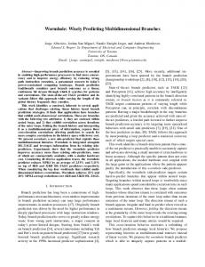
nonzero differential voltage is applied to the data inputs, the outputs will split and the positive feedback of the back-to-back inverters will eventually cause the sampler to latch with rail-to-rail values. If the differential input voltage is zero, however, the outputs will not split, and instead converge to an intermediate value (i.e., a zero differential output). The circuit can also become metastable when it is clocked during a data transition between two non zero, and opposite differential voltages. We define the sampling-time by the timing of a data transition, with respect to the clock edge, which results in a metastable output. In simulation, a noise impulse is applied to the power supply, and the clock timing is adjusted until the circuit is judged to be metastable. The adjustment of the clock timing is accomplished using the parameter optimization feature in Hspice; the clock timing is optimized to produce a minimum differential output voltage at a point in time sufficiently past the clock edge to demonstrate metastability. The change in clock timing caused by a noise impulse at time past the clock edge provides a point solution to . Full STSF characterization is then achieved by the STSF, sweeping the impulse time using multiple simulations. Fig. 6 shows the STSFs (in terms of picoseconds of sampling-time offset in response to the area (in volts picoseconds) under a perturbation impulse) of the three individual components in Fig. 4: The phase interpolator, the clock buffer, and the sampler. The STSF of the phase interpolator is much longer in duration than those of the clock buffer and the sampler. This indicates that the buffer and sampler are only sensitive to supply noise during their transient states (at the clock edges), while the phase interpolator has internal analog nodes that remain sensitive to noise throughout the clock cycle. The resulting greater area under the phase interpolator’s STSF implies that it is far more sensitive to supply noise.
(3) is the Fourier transform of . To determine where when , we can still use (3), but capture the noise sinusoid’s phase with an equivalent phase at . During an is then determined using (3) event-driven CDR simulation at each sample point. Because the STSF only needs to be extracted once for each design, the overhead of modeling the noise effects is limited to the evaluation of (3) once per sample. This approach can be extended to include the effect of periodic supply noise other than sinusoidal. In general, the convolution of the STSF and the noise waveform produces a solution for (1) over the entire noise period. This result is stored in a look-up table in the model, and the sampling-time offset block need only keep track of the current position within the noise waveform during each sample, and use this position as an index into the lookup-table. is introduced into the model In our event-driven model using the sampling-time offset block shown in Fig. 3(b). When a data transition occurs near the sample time, this allows the CDR model to determine if the supply noise changes the sampling time sufficiently to alter the sampler’s binary output. This will in turn change the early/late decision of the phase detector. Model Verification: To verify the accuracy of the model described above, we compare the sampling-time offset predicted by our model to the results of Hspice simulations using a sinu, with various soidal noise source of 100 mV and . The circuit we use for this verification is the phase interpolator within the clock path shown in Fig. 4, designed in a 0.11- m CMOS process. The results of this comparison are shown in Fig. 7, confirming the accuracy of our modeling approach. The results show a very
1310
IEEE TRANSACTIONS ON CIRCUITS AND SYSTEMS—I: REGULAR PAPERS, VOL. 55, NO. 5, JUNE 2008
produce this output condition, we can reconstruct the sampler’s impulse response. A set of input signals that satisfy this condition are of the form , where and can be determined for each so as to produce the metastable output. At the output of the , this input signal results in filter
(6) where is the dc component of . Since the input to the quantizer is the solution to (6) at the metastable output condition can only occur when
Fig. 7. MatLab versus HSpice simulated sample-time offset for various f
(7)
.
good agreement between the Hspice and Matlab simulations. In the worst case, for a 50-mV, 1-GHz sinusoidal supply noise our model predicts a peak jitter of 12.8 ps, compared to a peak jitter of 11.4 ps by Hspice—a 12% error. Note however, that the MatLab simulations complete in less than a second, while the Hspice simulations required many hours to complete. IV. SAMPLER IMPULSE RESPONSE An ideal sampler samples its input voltage instantaneously. In reality, the sampling is performed over a window of finite duration, known as the aperture window. We can describe this applied to the input voltage process by a sampling function at time
(4) , this produces the instanIn the ideal case, where . taneous sample This sampling function becomes easier to incorporate into a system level model if we apply a variable substitution to (4)
(5) where denotes the convolution operation. This shows that the to a filter with sampling process is equivalent to applying impulse response , followed by an ideal sampler triggered at time . This is depicted in Fig. 8, along with a quantization block that slices the sampled value into one of two logical levels (in the case of binary signaling). Our goal here is to find a such that the system shown in Fig. 8 will have the same inputoutput characteristics as that of the circuit shown in Fig. 5. can be determined if we Given an arbitrary input can extract , the output of the filter block, from the does not exist in the physical circuit of Fig. 5. However, circuit implementation, neither is it observable from the output becomes zero. At of the quantizer, except for when , the output of the quantizer is undefined and the output of the circuit becomes metastable. By finding a set of input signals that
,
This can be rearranged as
(8) constant, then beThis implies that if we keep , of the comes directly proportional to the dc component, input signal that causes the sampler to become metastable. Simulating to find this value provides the required indirect measure. ment of the filter for a given value of , we first perform To determine a simulation to find the amplitude of the dc level, , required to cause metastability. As in the previous section, our simulation uses Hspice optimization to find this metastable point. For with the goal of producing a difa given , we optimize ferential output voltage of zero. By sweeping the timing of the delta function, , across the sampler’s aperture window, and at each point determining , we determine the scaled and time reversed impulse response of the sampler. The exact value of the , is irrelevant, as the quantizer proportionality constant, output is a function of only the sample’s polarity. A flowchart summarizing this procedure is shown in Fig. 9. Fig. 10(a) shows the simulated voltages for the input, output and clock nodes of the sampler in Fig. 5, showing both the case of fully switched outputs, as well as metastable outputs. (and hence Fig. 10(b) shows the normalized value of ) found through simulation. The results show that the impulse response begins when the clock input reaches nMOS threshold voltage ( 400 mV), turning on the clocked nMOS device, and ends when the output nodes drop by a pMOS threshold voltage ( 400 mV), turning on the pMOS devices of the back-to-back inverters. The reader notes that Fig. 10(a) shows only one of many simulations used to derive the impulse response shown Fig. 10(b). The purpose of their juxtaposition in this figure is to illustrate the timing relationship between the impulse response and the clock timing of the latch. The input of the latch can only influence its output within the time window of the impulse response [Fig. 10(b)]. To implement this modeling technique in an event-driven CDR simulation, the filter modeling the finite bandwidth of the sampler is combined with the filter modeling the lossy data
VAN IERSSEL et al.: EVENT-DRIVEN MODELING OF CDR JITTER
1311
Fig. 8. Model of sampler.
Fig. 9. Extraction procedure of sampler’s impulse response.
Fig. 11. Model verification. (a) Simulation testbench. (b) Simulation results.
Fig. 10. Sampler. (a) Node voltages. (b) Normalized impulse.
channel as the data filter shown in Fig. 3(b). The implementation of this combined filter is discussed in Section V. Model Verification: To verify our model, we test it with waveforms representative of what would be experienced when the sampler is integrated into a CDR. The only sampler outputs that are of interest in this case are those that could produce either a high or a low output given a small perturbation, that is, when the sampler is clocked near transitions in its input data signal. Our verification simulations examine the output of our sampler when clocked near data transitions, using varying transition
, to emulate the data dependent slew rate resulting times, from channel ISI. The simulation testbench is illustrated in Fig. 11(a). A data signal that is transitioning between data 0 and data1 is applied to the simulated sampler, along with a rising clock edge. This setup is then simulated, using Hspice, to determine the , required to generate a metastable sampling-time offset, output. We then determine the sampling-time offset again, this time by convolving the impulse response we previously extracted with the data signal, and locating the zero-crossing. This comparison is performed for varying data transition times, and the results are illustrated in Fig. 11(b). The upper- left and lower-right portions of the figure show the timing regions where both methods indicate that the sampler will output data1 and data0, respectively. The shaded region in the center shows where the methods disagree, with its upper and lower boundary curves denoting the metastability points for the Hspice and impulse response models, respectively. In other words, for all and , both Hspice and Simulink combinations of produce the same Q output, except for the points residing in the gap (the shaded area). This gap corresponds to less than 0.3 ps
1312
IEEE TRANSACTIONS ON CIRCUITS AND SYSTEMS—I: REGULAR PAPERS, VOL. 55, NO. 5, JUNE 2008
Fig. 13. Step response samples versus Hspice simulation.
Substituting this into (9) allows us to express the filter output as (11)
Fig. 12. Data filter. (a) Conceptual system. (b) Implementation based on step response.
of timing error. This is expected to result in a jitter prediction error of similar magnitude in the CDR simulation.
V. EVENT-DRIVEN IMPLEMENTATION OF THE DATA FILTER This section describes the event-driven implementation of the data filter in Fig. 3(b). As shown in Fig. 12(a), this filter models the ISI from the lossy data channel and the limited bandwidth of the phase-detector samplers. Formally, its effect on the received data sequence can be represented by
(9) is convolved with the comwhere the transmitted signal bined impulse response of the data channel and phase detector to generate the input to the idealized CDR sampler. Unlike discrete time filter implementations, the filter implementation required in a CDR operates in the presence of jitter and changing cycle times. Because of the resulting irregular time steps, a filter implementation using z-domain techniques is not possible. Instead, we calculate the filter output using the of the system and exploit the fact that the step-response transmitted signal is not an arbitrary waveform, but rather a series of pulses of nonuniform duration. In other words, we can as the following: express
(10) where is the th transmitted data symbol, is the ideal step function, and and are the start and end times of the symbol, respectively.
Since the step response is usually limited to only a few bit periods in duration, we only need to evaluate the first few elements in this summation. In addition, the step response can be predetermined and stored in a lookup table for use during simulation. Since we use binary signaling and normalize the transto , the filter implementation is mitted data symbols reduced to a small number of table lookups and additions (or subtractions). A block-level implementation of this concept is shown in Fig. 12(b), where the summation in (11) is simplified to only include the effect of the previous data symbols. The computation can be further simplified by realizing that the table lookups required for the trailing edge calculation are a subset of those required for the leading edge contribution and can be shared. Note that in the trailing edge calculation we discard the current data bit because, by definition, its trailing edge has not yet occurred. The summation of the leading and trailing edge contributions produces the signal level at the input to the receiver’s ideal sampler. ISI Model Verification: To verify our model, we use it to predict the output of a data channel with a random data sequence applied to it. These results are then compared to the output of an Hspice simulation of the same system. The result of this simulation is shown in Fig. 13 where the continuous waveform is the Hspice output, and the crosses are the sample values determined using the step response model. The RMS error for the data samples is 1.1%. Most of the error is due to the truncated in this example), and could summation used in Fig. 12 ( be reduced at the expense of increased computation. VI. PUTTING IT ALL TOGETHER—SYSTEM-LEVEL SIMULATION RESULTS In previous sections, we examined CDR modelling at a component level. In this section, we incorporate these component models in a complete event-driven CDR model. We then compare the simulated jitter in our event-driven CDR model to the jitter in Hspice simulations of the same CDR. This model comparison is performed in two parts: First, we evaluate the use of the sampling-time offset to capture jitter due to supply noise. Second, we evaluate the use of the event-driven data filter to capture jitter due to limited bandwidth in the channel and in the phase-detector samplers.
VAN IERSSEL et al.: EVENT-DRIVEN MODELING OF CDR JITTER
1313
The CDR being modelled uses the architecture described in Section II, operating at 3.2 Gbps. It uses 2x oversampling phase detection, built around the sampler shown in Fig. 5. The loop filter is a first-order digital low-pass filter, with a bandwidth of 4 MHz. The phase interpolator is built using a current-starved inverter architecture [15], and interpolates an ideal 3.2-GHz clock to generate the local clock. The local clock is then supplied to the phase detector through an inverter-based clock buffer. The channel model used in this system has a first-order response, with a 3-dB bandwidth of 1.6 GHz. The event-driven model of the above CDR is implemented in Matlab’s Simulink [17] using the structure shown in Fig. 3(b). The data filter block is structured in the manner described in Section V. The impulse response of this filter is the convolution of the channel and sampler impulse responses, where the sampler impulse response is determined using the process described in Section IV. The sampling-time offset block is implemented using the technique described at the end of Section III for periodic supply noise waveforms.
Fig. 14. Clock jitter due to FM supply noise for Hspice and Simulink simulations.
A. Clock Jitter due to Supply Noise In this section, we compare our event-driven model in Matlab against Hspice simulations in predicting jitter in the recovered clock due to supply noise. For these simulations we choose an FM-modulated supply noise
(12) 0.1 V That is, an FM noise having a peak amplitude of 3.2 GHz (the with the noise frequency centered around f CDR’s bit rate) and FM modulation with a peak frequency de500 MHz, and with a modulation frequency of viation of 5 MHz. This FM noise source allows the demonstration of two properties: First, while the sampling-time offset can be determined as a continuous time function by convolving the FM noise source with the circuit’s STSF, it is only sampled during the clock edge events. This results in the aliasing of the noise down to a frequency band centered around dc. Second, as shown in Fig. 7, the sampling-time offset sensitivity drops to less than half of its low-frequency value between 1 GHz and 4 GHz, overlapping the range of instantaneous frequencies of the FM noise source. The implication of this is that while noise at 2.7 and at 3.7 GHz will both be aliased to 500 MHz, the sampling-time offset due to the 3.7-GHz noise will be attenuated compared to that of the 2.7-GHz noise. The effects of these properties can be seen in Fig. 14, where the top curve shows the instantaneous frequency of the FM noise source, the middle and bottom curves show the jitter in the recovered clock determined using Hspice and event-driven simulations, respectively. The effect of the aliasing can be seen in both simulations where the jitter frequency in the CDR output goes through zero when the instantaneous noise frequency equals 3.2 GHz. It can also been seen that the jitter amplitude is lower in both simulations at the higher instantaneous noise frequencies.
Fig. .15. Clock jitter due to limited channel bandwidth for Hspice and Simulink channel simulations.
B. Clock Jitter due to Limited Bandwidth This section compares the simulated jitter due to limited bandwidth as modeled by the data filter block in our event-driven model to the jitter predicted by an equivalent Hspice simulation. We perform this comparison in two steps: First, we look at the jitter due to limited bandwidth in the channel in order to verify the performance of the data filter block. Second, we examine jitter due to limited bandwidth in the phase detector’s samplers to verify the characterization of their impulse response. To demonstrate jitter due to limited bandwidth, we choose a data sequence that begins with a repeating sequence of “11110000” switching to “10101010” after 100 ns. During transmission of the first sequence, ISI in the received signal will cause the signal transitions to be delayed compared to the signal transitions occurring during transmission of the second sequence. The CDR should track this change of transition location, producing jitter in the recovered clock.
1314
IEEE TRANSACTIONS ON CIRCUITS AND SYSTEMS—I: REGULAR PAPERS, VOL. 55, NO. 5, JUNE 2008
TABLE I SIMULATION TIME
which is 1800 times faster than Hspice and 7.5 times faster than the fixed-time-step simulation. VII. CONCLUSION
Fig. 16. Clock jitter due to limited sampler bandwidth for Hspice and Simulink sampler simulations.
The simulated jitter due to limited bandwidth in the channel is shown in Fig. 15. The top waveform shows the transmitted data pattern, while the middle and bottom waveforms show the jitter in the recovered clock for the Hspice and event-driven simulations, respectively. Both simulations show the roughly the same 60-ps change in recovered clock phase. To demonstrate the jitter due to limited bandwidth in the phase detector samplers, characterized in Section IV, we artificially introduced large parasitic capacitors into the samplers to exaggerate their impulse response. Simulation results using the data filter to model the limited bandwidth of the modified samplers are shown in Fig. 16. The top waveform shows the same transmitted data pattern as before, while the middle and bottom waveforms show the jitter of the recovered clock for the Hspice and event-driven simulations, respectively. Once again, there is a good correspondence between the jitter predictions, roughly 8 ps, in both simulations. Despite the similar behavior of CDR jitter as obtained by Hspice and Simulink, there are some differences in their waveforms (both in Figs. 14 and in 15). For example, we observe from Fig. 14 that the CDR jitter shows a jitter period in Simulink that is slightly different from its corresponding jitter in Hspice. This, and other small differences, suggest that Simulink results should only be used as a measure of CDR “behavior”, and not as a total replacement for Hspice results. C. Simulation Time While the previous section demonstrated the accuracy of our event-driven CDR simulation techniques, the real advantage of these techniques becomes apparent when comparing the simulation time required by the two techniques. As shown in Table I, simulating the CDR to reproduce the results shown in Fig. 14 for about 600 cycles in Hspice takes 2 h, while the same simulation using a conventional fixed-time-step model with a step size of 1/32th of the nominal bit rate requires 30 s —a 240x speed up. In comparison, the event-driven model takes only 4 s,
This paper presented event-driven CDR simulation techniques that allow the quick and accurate prediction of jitter in the recovered clock. These techniques introduce the modeling of supply noise, the characterization of bandwidth limitations in the phase detector samplers, and a discrete-time filter implementation for nonuniform time intervals. The supply noise can be modeled as a sampling-time offset in the phase detector samplers. This sampling-time offset is determined by taking the dot product of the supply noise waveform and the STSF of the circuit. We describe the process for characterizing the STSF of the circuit. The limited bandwidth of the phase detector samplers can be modeled as a filter preceding an ideal sampler. The process of characterizing the impulse response of this filter is presented. A discrete-time filter for nonuniform time steps can be implemented by describing the transmitted data sequence as a sequence of rising and falling steps, instead of pulses, and applying the system’s step-response to each step. This process simplifies the computation of received sample values to only a few operations. The event-driven modeling techniques presented in this paper offer a simulation accuracy close to that of Hspice, but with a simulation speed up of 1800 times. This was confirmed through a CDR simulation in both. ACKNOWLEDGMENT The authors wish to thank the anonymous reviewers for their excellent comments and contributions to this manuscript. REFERENCES [1] M. Horowitz, K. Yang, and S. Sidiropoulos, “High-speed electrical signaling: Overviews and limitations,” IEEE Micro, pp. 12–24, Jan.–Feb. 1998. [2] H. Kobayashi, K. Kobayashi, and M. Morimura, “Sampling jitter and finite aperture time effects in wide-band data acquisition systems,” IEICE Trans. Fundam., pp. 335–346, Feb. 2002. [3] Y. Okaniwa, H. Tamura, and M. Kibune, “A 40-Gb/s CMOS clocked comparator with bandwidth modulation technique,” IEEE J. Solid-State Circuits, vol. 40, no. 8, pp. 1680–1687, Aug. 2005. [4] P. Larsson, “Measurements and analysis of pll jitter caused by digital switching noise,” IEEE J. Solid-State Circuits, vol. 36, no. 7, pp. 1113–1119, Jul. 2001. [5] P. Heydari and M. Pedram, “Analysis of jitter due to power-supply noise in phase-locked loops,” in Proc. IEEE Custom Integr. Circuits Conf., 2000, pp. 443–446.
VAN IERSSEL et al.: EVENT-DRIVEN MODELING OF CDR JITTER
1315
[6] N. Ou, T. Farahmand, A. Kuo, S. Tabatabaei, and A. Ivanov, “Jitter models for the design and test of gbps-speed serial interconnects,” IEEE Design Test Comput., vol. 21, no. 4, pp. 302–313, Jul.–Aug. 2004. [7] J. Buckwalter and A. Hajimiri, “Analysis and equalization of data-dependent jitter,” IEEE J. Solid-State Circuits, vol. 41, no. 3, Mar. 2006. [8] B. Lai and R. Walker, “A monolithic 622 Mb/s clock extraction data retiming circuit,” in IEEE Int. Solid-State Circuits Conf. Dig. Tech. Papers, Feb. 1991, pp. 144–145. [9] M. H. Perrott, “Fast and accurate behavioral simulation of fractionalfrequency synthesizers and other PLL/DLL circuits,” in Proc. IEEE Design Automation Conf. (DAC), Jun. 2002, pp. 498–503. [10] M. Perrott, M. Trott, and C. Sodini, “A modeling approach for 61 fractional- frequency synthesizers allowing straightforward noise analysis,” IEEE J. Solid State Circuits, vol. 37, no. 8, pp. 1028–1038, Aug. 2002. [11] Demir, E. Liu, A. L. Sangiovanni-Vincentelli, and I. Vassiliou, “Behavioral simulation techniques for phase/delay-locked systems,” in Proc. IEEE Custom Integr. Circuits Conf., 1994, pp. 453–456. [12] J. Kim, Y. Lu, and R. Dutton, “Modeling and simulation of jitter in phase-locked loops due to substrate noise,” in Proc. IEEE Behav. Model. Simul. Workshop (BMAS), Sep. 2005, pp. 25–30. [13] “Star-hspice manual,” Avant! May 2000. [14] R. Jain, The Art of Computer Systems Performance Analysis. New York: Wiley, 1991, pp. 406–408. [15] H. Takauchi and H. Tamura, “A CMOS multichannel 10-Gb/s transceiver,” IEEE J. Solid-State Circuits., vol. 38, no. 12, pp. 2094–2100, Dec. 2003. [16] A. Hajimiri and T. H. Lee, “A general theory of phase noise in electrical oscillators,” IEEE J. Solid-State Circuits, vol. 33, no. 2, Feb. 1998, Using Simulink, The Mathworks Inc., July 2002.. [17] Using Simulink. Natick, MA: The Mathworks Inc., Jul. 2002.
N
N
Marcus van Ierssel (S’92–M’07) received the B.A.Sc. degree in electrical engineering from the Division of Engineering Science, the M.A.Sc. degree in the electrical and computer engineering, and the Ph.D. degree in the electrical and computer engineering all from the University of Toronto, Toronto, ON, Canada, in 1992, 1995, and 2007, respectively. He is currently working at Snowbush Microelectronics, Toronto, ON, Canada as an Analog IC Designer, focusing on phase-locked loop and SERDES design.
Hisakatsu Yamaguchi received the graduate degree in electrical engineering from the Tokyo University of Science, Chiba, Japan, and the M.S. degree in electrical engineering from the University of Tokyo, Tokyo, Japan,in 1994, and 1996, respectively. In 1996, he joined Fujitsu Laboratories. Ltd., Kawasaki, Japan, where he has been engaged in research on DRAMs with high-speed IFs and has been responsible for developing MPEG4 Codec LSIs. He is currently working on developing high-speed IFs.
Ali Sheikholeslami (S’98–M’99–SM’02) received the B.Sc. degree from Shiraz University, Shiraz, Iran, in 1990 and the M.A.Sc. and Ph.D. degrees from the University of Toronto, Toronto, ON, Canada, in 1994 and 1999, respectively, all in electrical and computer engineering. In 1999, he joined the Department of Electrical and Computer Engineering, University of Toronto, where he is currently an Associate Professor. His research interests are in the areas of analog and digital integrated circuits, high-speed signaling, and VLSI memory design (including SRAM, DRAM, CAM, and FeRAM). He has collaborated with industry on various VLSI design research in the past few years, including work with Nortel and Mosaid, Canada, and with Fujitsu Labs. He spent his 2005–2006 research sabbatical year with Fujitsu Labs of Japan and Fujitsu Labs of America. He presently supervises two active research groups in the areas of high-speed signaling and VLSI memories. He has coauthored several journal and conference papers (in both areas), in addition to three US patents on VLSI memories. Dr. Sheikholeslami served on the Memory Subcommittee of the IEEE International Solid-State Circuits Conference (ISSCC) from 2001 to 2004, and on the Technology Directions Subcommittee of the same conference from 2002 to 2005. He presented a tutorial on ferroelectric memory design at the ISSCC 2002. He was the program chair for the 34th IEEE International Symposium on Multiple-Valued Logic (ISMVL 2004) held in Toronto, Canada. He is a registered professional engineer in the province of Ontario, Canada. Dr. Sheikholeslami received the Best Professor of the Year Award in 2000, 2002, and 2005 by the popular vote of the undergraduate students in the Department of Electrical and Computer Engineering, University of Toronto. In 2006, he received the Early Career Teaching Award in recognition of his “superb accomplishment in teaching” from the Faculty of Applied Science and Engineering at the University of Toronto.
Hirotaka Tamura (M’02) received the B.S., M.S., and Ph.D. degrees in electronic engineering from Tokyo University, Tokyo, Japan, in 1977, 1979, and 1982, respectively. In 1982, he joined Fujitsu Laboratories, Ltd., Kawasaki, Japan, where he was engaged in research on Josephson devices and other exploratory devices. In 1995, he moved into the area of CMOS circuit design. After working on multi-gigabit DRAMs and ferroelectric nonvolatile memories, he got involved in CMOS high-speed signaling. His current interest covers the circuit topology and architecture of high-speed CMOS interfaces.
William W. Walker (M’79) received the A.B. degree in physics and applied math in 1976, and the M.S.E.E. degree in 1978, both from the University of California at Berkeley. From 1978 to 1983, he was a Staff Engineer at IBM Corporation, East Fishkill, NY, and Burlington VT, where he was involved in the development of the LDD MOS transistor. From 1984 to 1991 he was a Senior Engineer at Integrated CMOS Systems, Inc. in Sunnyvale CA. From 1991 to 2000, he was an Engineering Manager at Hal Computer Systems, Inc. in Campbell, CA where his group developed CAMs, SRAMs, PLLs, and Register Files for the first 64-bit SPARC microprocessors. Since 2000, he has been employed at Fujitsu Laboratories of America, where he is currently Vice President in charge of the Circuits and Devices Innovation Group. His research interests include high-speed and low-power digital circuits for microprocessors, millimeter-wave CMOS, and high-speed wireline CMOS circuits for computer backplanes and optical communications.