M PRA Munich Personal RePEc Archive
Energy consumption and economic growth: evidence from nonlinear panel cointegration and causality tests Tolga Omay and Mubariz Hasanov and Nuri Ucar Cankaya University Economics Department, Hacettepe University Economics Department, Cankaya University Economics Department
26. March 2012
Online at http://mpra.ub.uni-muenchen.de/37653/ MPRA Paper No. 37653, posted 26. March 2012 14:15 UTC
Energy Consumption and Economic Growth: Evidence from Nonlinear Panel Cointegration and Causality Tests Tolga OMAY (Corresponding Author) Çankaya University, Department of Economics, Ankara, Turkey Phone: +90 312 233 1190 -91-92 Fax: +90 312 233 1195, e-mail:
[email protected] Mübariz HASANOV Hacettepe University, Faculty of Economics and Administrative Sciences, Department of Economics, Beytepe, Ankara, Turkey, Phone: +90 312 297 8652 (Extension 114), e-mail:
[email protected] Nuri UCAR Hacettepe University, Faculty of Economics and Administrative Sciences, Department of Economics, and Çankaya University Vocational School, Foreign Trade Department, Ankara, Turkey Phone: +90 : +90 312 233 1190 -93 Fax: +90 312 233 1195, e-mail:
[email protected]
Abstract
In this paper, we propose a nonlinear cointegration test for heterogeneous panels where the alternative hypothesis is an exponential smooth transition (ESTAR) model. We apply our tests for investigating cointegration relationship between energy consumption and economic growth for the G7 countries covering the period 1977-2007. Moreover, we estimate a nonlinear Panel Vector Error Correction Model in order to analyze the direction of the causality between energy consumption and economic growth. By using nonlinear causality tests we analyze the causality relationships in low economic growth and high economic growth regimes. Furthermore, we deal with the cross section dependency problem in both nonlinear panel cointegration test and nonlinear Panel Vector Error Correction Model.
Keywords: Nonlinear panel cointegration, nonlinear Panel Vector Error Correction Model, cross section dependency JEL Classification: C12, C22
1. Introduction
The relationship between energy consumption and economic growth has been one of the most investigated yet controversial issues in the energy economics literature since the seminal work of Kraft and Kraft (1978). The interest of energy economists on this issue gained a new momentum with increasing concerns about global warming, especially after adoption of the Kyoto Protocol in 1997 that entered into force in 2005. Industrialized member countries committed themselves to a reduction of greenhouse gas emission, mainly by restricting fossil fuel consumption. However, since energy is considered as an essential factor of production by many energy economists (e.g., Stern, 2000; Oh and Lee, 2004; Ghali and El-Sakka, 2004, Beaudreau, 2005, Lee and Chang, 2008), it is argued that reducing energy consumption may hamper economic growth and hence increase unemployment. On the other hand, the proponents of the so-called “conservation hypothesis” argue that the positive relationship between energy consumption and output level stems from positive effects of output growth rate on energy consumption, and hence policies aimed at conserving energy consumption will have only a limited, if any, adverse effect on economic growth. Similarly, supporters of the “neutrality hypothesis” argue that energy consumption and output level are not correlated, and therefore neither energy conservation nor energy promoting policies will affect economic growth of countries (see, for example, Lee and Chang, 2008; Apergis and Payne, 2009; Ozturk, 2010). Taking account of these alternative views regarding the relationship between energy consumption and output level, it is evident that discovering the causal linkages between energy consumption and economic growth is vital in designing energy policies for each nation. Although the causal relationship between economic growth and energy consumption has been investigated extensively in the literature, no consensus has been reached yet (see, for instance, a recent literature survey by Ozturk, 2010). Stern (2000), Oh and Lee (2004), Wolde-Rufael (2004), Ho and Siu (2007), among others, argue that only energy consumption leads output growth. On the other hand, Zamani (2007), Mehrara (2007), Ang (2008), Zhang and Cheng (2009) argued that causality runs from output to energy consumption, in accordance with the conservation hypothesis. Glasure (2002), Erdal et al. (2008) and Belloumi (2009) found a bi-directional causality between the energy consumption and output level. However, Halicioglu (2009) and Payne (2009) found no causality between energy consumption and output. Soytas and Sari (2003), Lee (2006), Francis et al. (2007), Akinlo (2008), Chiou-Wei et al. (2008) found mixed results for various groups of countries. Conflicting results in the empirical literature have usually been attributed to use of different time periods, sample countries, econometric methods, and functional forms (e.g., Soytas and Sari, 2003; Lee, 2006; Ozturk, 2010, Balcilar et al. 2010, Costantini and Martini, 2010). Modelling possible
nonlinear relationships between economic variables has attracted huge interest of economists, and a growing body of empirical work is being devoted to examination of possible nonlinear causal relationships between energy consumption and output level. Recent studies of Hamilton (2003), Chiou-Wei et al. (2008), Huang et al. (2008), Aloui and Jammazi (2009), Gabreyohannes (2010), Rahman and Serletis (2010), among others, imply that the interrelationship between energy consumption and economic variables might be inherently nonlinear. Chiou-Wei et al. (2008) examined causality between energy consumption and output in the case of eight Asian countries and the USA using linear and nonlinear causality tests. They found that the implied direction of causality between energy consumption and output in the cases of Taiwan, Singapore, Malaysia and Indonesia is reversed when possible nonlinearity in the interrelationship between the variables is allowed for. However, both the linear and nonlinear causality tests suggest the same direction of causality or non-causality in the cases of Korea, Hong-Kong, Philippines, Thailand and the USA. Huang et al. (2008) examined nonlinear relationships between energy consumption and economic growth for 82 countries using threshold regression models. Using various candidates for the regime-switching variable they found significant positive relationship between energy consumption and output growth for regimes associated with lower threshold values. However, when the threshold variables are higher than certain threshold levels, they found either no significant relationship or a significant but negative relationship between energy consumption and economic growth. Hamilton (2003) examined nonlinear relationship between oil price changes and GDP, and found clear evidence of nonlinearity. His results suggest that oil price increases affect GDP much more than oil price decreases. Aloui and Jammazi (2009) examined the relationship between crude oil shocks and stock markets in the case of the UK, Japan, and France using Markov switching EGARCH models. They found that the responses of the real stock market return volatilities to crude oil shocks are regime dependent in all three markets. Gabreyohannes (2010) examined the effects of price change on electricity consumption using nonlinear smooth transition regression (STR) modelling approach, and found that changes in electricity prices affect residential electricity consumption in Ethiopia asymmetrically. In a similar framework, Rahman and Serletis (2010) examined asymmetric effects of oil price shocks and monetary shocks on macroeconomic activity using multivariate STR model for the USA. They found that both the oil prices and oil price volatility affect output nonlinearly. Cheng-Lang et al. (2010) examined causality between sectoral electricity consumption in Taiwan using linear and nonlinear causality tests and found nonlinear bi-directional causality between
total electricity consumption and output level, and unidirectional nonlinear causality from output level to residential electricity consumption. Lee and Chang (2007) and Huang et al. (2008) examined energy consumption output growth causality by separating countries into different groups by level of development and found that the direction of causality varies with level of development. Their results suggest that the causality between energy consumption and output level is not linear, and depends on output level. In addition, Moon and Sonn (1996) argued that economic growth rate rises initially with productive energy expenditures but subsequently declines. In other words, according to Moon and Sonn (1996), there is an inverse Ushaped nonlinear relationship between energy consumption and economic growth. Our main aim in this paper is to investigate nonlinear causal relationship between energy consumption and output growth rate in the case of G7 (group of seven) countries. The G7 countries are the most industrialized countries that play a crucial role in global economy, and have comparable level of economic development. In addition, these countries’ share in total carbon dioxide emission accounted for around 32.2% in 2007 according to calculations of Carbon Dioxide Information Analysis Center (CDIAC) of the US Department of Energy (Boden et al., 2010). In recent years, the G7 countries have followed policies aimed at reducing total greenhouse gas emissions. Therefore, it is important to discover all aspects of the causal relationship between energy consumption and output for these countries. Soytas and Sari (2003; 2006), Zachariadis (2007), Narayan et al. (2007), Narayan and Smyth (2008), Lee and Chien (2010), among others, have examined the energy consumption and output growth causality for the G7 countries, and found mixed results. Soytas and Sari (2003; 2006), Zachariadis (2007) and Lee and Chien (2010) used various multivariate cointegration and causality tests. On the other hand, Narayan et al. (2007) and Narayan and Smyth (2008) applied panel cointegration techniques. Although we also use panel data techniques, our approach in this paper is different from previous studies from several perspectives. The main novelty of the paper is that, we propose a nonlinear panel cointegration and causality tests in order to investigate the causal relationship between energy consumption and real output level. Another contribution of the paper is that we estimate a nonlinear panel error correction model that allows for smooth changes between regimes as well as examining causal relationship in each regime separately. Discovering regime-dependent interactions between the energy consumption and output is also crucial for designing more appropriate energy policies. In addition, we propose a new method to remedy the cross section dependency problem in both linear and nonlinear panel regression models.
We first apply linear and nonlinear panel unit root tests to investigate stationarity properties of energy consumption and real output level, and discover that both series follow a non-stationary unit root process. Then we develop a nonlinear panel cointegration test, and apply this test to the data under consideration. Although linear panel cointegration test of Pedroni (2004) indicate no cointegration relationship among the series, we find a strong evidence of cointegration after allowing for nonlinearity in the long-run relationship. Then we estimate a nonlinear panel vector error correction model in order to investigate the short-run causalities between energy consumption and real output. For this purpose, we propose a regime-wise Granger-causality test for a nonlinear panel regression model, and examine the causal relationship between the variables for each regime separately. The remaining of the paper is structured as follows. In the next Section 2 we describe our newly proposed nonlinear panel cointegration and causality tests as well as panel error correction model. In Section 3 we provide results of the tests, and then Section 4 concludes.
2. Econometric Methodology
Although several plausible nonlinear models have been used in the empirical economics literature, we prefer smooth transition regression (STR) modelling approach. The STR modelling approach has several advantages over other nonlinear models (see, for example, Teräsvirta and Anderson, 1992; Granger and Teräsvirta, 1993). First, STR models are theoretically more appealing over simple threshold and Markov regime switching models, which impose an abrupt change in coefficients. Instantaneous changes in regimes are possible only if all economic agents act simultaneously and in the same direction. Second, the STR model allows for modelling different types of nonlinear and asymmetric dynamics depending on the type of the transition function. In particular, a STR model with a first-order logistic transition function is more convenient for modelling the interaction between energy consumption and output growth rate if the dynamic interrelationships between the variables depend on the phases of business cycles. On the other hand, a STR model with an exponential or second-order logistic transition function is more convenient if, for example, the interaction between the variables depend not on the sign but on the size of fluctuations in variables. Finally, STR modelling approach allows one to choose both the appropriate switching variable and the type of the transition function unlike other regime switching models that impose both the switching variable and function a priori. Now we briefly discuss nonlinear panel cointegration and causality tests as well as panel error correction model.
2.1. Nonlinear Panel Cointegration Test
Consider following panel regression model: where y i ,t and
xi ,t
y i ,t = a i + b i x i ,t + u i ,t denote observable I (1) variables, b = ( b 1 , ..., b m )
(1) are parameters to be
estimated, and u i ,t is the error term. y i ,t is scalar, and x i ,t = (x 1,t , x 2,t , ..., x m ,t ) is an (m x1) vector and finally a i is fixed effect (heterogeneous intercept). We assume that an (n x1) vector
zi' ,t º (y i ,t , xi' ,t ) is generated as zi ,t = zt - 1 + ei ,t , where ei ,t are i.i.d. with mean zero, positive definite variance-covariance matrix å , and E ei ,t
s
< ¥ for some s > 4 .
If the error term u i ,t in regression (1) is stationary, then vector zi ,t is said to be co-integrated, and u i ,t is called equilibrium error (Engle and Granger, 1987). In this paper, we assume that u i ,t can be modelled using following nonlinear model: where xi ,t
(2) u i ,t = gi u i ,t - 1 + y i u i ,t - 1F (u i ,t ; qi ) + xi ,t is a zero mean error and F (u i ,t ; qi ) is a smooth transition function of u i ,t - 1 . Note that by
imposing F (u i ,t ; qi ) = 0 or F (u i ,t ; qi ) = - g i mi ' where mi ' is vector of level parameters, one obtains conventional linear cointegration equation (e.g., Kapetanois et al., 2006) Following earlier literature on nonlinear unit root and cointegration (e.g., Kapetanois et al., 2003, 2006; Uçar and Omay, 2009, Maki, 2010) we assume that the transition function F (u i ,t ; qi ) is of the exponential form1:
F (u i ,t ; qi ) = 1 - exp{- qi u i2,t - 1 }
(3)
Here it is further assumed that u i ,t is a mean zero stochastic process and that qi ³ 0 . The transition function F (u i ,t ; qi ) is bounded between zero and one, and is symmetrically U-shaped around zero. The parameter qi determines the speed of the transition between the two extreme values of the transition function2 F (u i ,t ; qi ) . The exponential transition function has a nice property in that it allows for adjustment to the long-run equilibrium depending on the size of the disequilibrium. Substituting (3) in (2) and re-parameterising the resultant equation, we obtain following regression model:
1
Kapetanois et al. (2003, 2006) show that both second-order logistic and exponential functions give rise to the same auxiliary regression for testing the cointegration. 2 For a thorough discussion of smooth transition regression models and properties of transition functions, see, for example, Granger and Teräsvirta (1993) and Teräsvirta (1994).
D u i ,t = j i u i ,t - 1 + y i u i ,t - 1 éê1 - exp{- qi u 2i ,t - 1 }ùú+ ei ,t (4) ë û If qi > 0 , then it determines the speed of mean reversion. If j i ³ 0 , this process may exhibit unit root or explosive behaviour for small values of u i2,t - 1 . However, if the deviations from the equilibrium are sufficiently large (i.e., for large values of u i2,t - 1 ), it has stable dynamics, and as a result, is geometrically ergodic provided that j i + y i < 0 3. Imposing j
i
= 0 (implying that u i ,t follows a unit root process in the middle regime) and
further allowing for possible serial correlation of the error term in (4) we obtain the following regression model:
D u i ,t = y i u i ,t - 1 éê1 - exp{- qi u 2i ,t - 1 }ùú+ ë û
p
å
r ij D u i ,t - j + ei ,t
(5)
j= 1
Test of cointegration can be based on the specific parameter qi , which is zero under the null hypothesis of no-cointegration, and positive under the alternative hypothesis. However, direct testing of the null hypothesis is not feasible, since y i is not identified under the null. To overcome this problem, following Luukkonen et al. (1988), one may replace the transition function
F (u i ,t ; qi ) = 1 - exp{- qi u i2,t - 1 } with its first-order Taylor approximation under the null, which results in the following auxiliary regression model: pi
D u i ,t = di u i3,t - 1 +
å
r ij D u i ,t - j + ei ,t
(6)
j= 1
where ei ,t comprises the original shocks ei ,t in equation (5) as well as the error term resulting from Taylor approximation. Note that we allow for different lag order pi for each entity in regression equation (6). Now, the null hypothesis of no cointegration and the alternative can be formulated as:
H 0 : δ i = 0 , for all i, (no cointegration) H 0 : δ i < 0 , for some i,(Non-linear cointegration) In empirical application, one may select the number of augmentation terms in the auxiliary regression (6) using any convenient lag selection method. Following Ucar and Omay (2009), the cointegration test can be constructed by standardising the average of individual cointegration test statistics across the whole panel. The cointegration test for the ith individual is the t-statistics for testing δ i = 0 (as in Kapetanois et al., 2003 and Ucar and Omay, 2009) in equation (6) defined by:
3
For ergodicity of such nonlinear processes, see Kapetanois et al. (2003) and Ucar and Omay (2009).
ti , NL =
∆ui' M t ui3,−1
σˆ î , NL ( ui' , −1M t ui ,−1 )
(7)
3/ 2
(
where σˆ i2,NL is the consistent estimator such that σˆ i2, NL = ∆ui' M t ui /(T − 1) , M t = IT − τ T τ T' τ T
)
−1
τ T'
'
with ∆ui = ( ∆ui −1 , ∆ui − 2 ,...∆ui −T ) and τ T = (1,1,...,1) . Furthermore, when the invariance property and the existence of moments are satisfied, the usual normalization of tNL statistic is obtained as follows:
Ζ NL =
N ( tNL − E (ti , NL ) ) var(ti , NL )
(8)
N
where tNL = N −1
∑t
NL
, and E (ti , NL ) and var(ti , NL ) are expected value and variance of the ti , NL
i =1
statistic given in (7). One of the frequently encountered problems in panel regression models is the presence of cross-section dependency. The cross-section dependency may arise due to spatial correlations, spillover effects, economic distance, omitted global variables and common unobserved shocks (see, e.g., Omay and Kan, 2010). The presence of correlated errors through individuals makes the classical unit root and cointegration testing procedure invalid in panel data models. Banerjee et al. (2004) assess the finite sample performance of the available tests and find that all tests experience severe size distortions when panel members are cointegrated. To overcome this issue, some tests based on the regression equation including the unobserved and/or observed factors as the additional regressors are suggested in recent years (e.g., Moon and Perron, 2004; Bai and Ng, 2004; Pesaran, 2007; Bai et al. 2009;Omay and Kan, 20104; Kapetanios et.al., 2011). On the other hand, Maddala and Wu (1999), Chang (2004) and Ucar and Omay (2009) consider the bootstrap based tests to obtain good size properties. Therefore, before the testing procedure is implemented, one must check out the presence of cross section dependency, for example, using the test procedure proposed by Pesaran (2004). It is formulated as:
CD =
N −1 N 2T ∑ ∑ ρˆ ij N ( N − 1) i =1 j =i +1
(9)
where ρˆ ij is the estimated correlation coefficient between error terms for the individuals i and j . In this paper we followed and Ucar and Omay (2009) and applied the Sieve bootstrap method to deal with the cross-section dependency problem. Once cointegration is found and long-run 4
Omay and Kan (2010) proposed nonlinear CCE estimator as an extension of Pesaran (2007) linear CCE estimator.
relationship between the variables is established, one may proceed to estimate panel error correction model. Taking account of the fact that not only adjustment to the long-run equilibrium level, but dynamic interrelationship between the variables might also be inherently nonlinear, we propose and estimate nonlinear Panel Smooth Transition Vector Error Correction (PSTRVEC) model to examine regime-wise interactions between energy consumption and output growth. Now, we turn to discussion of specification and estimation of PSTRVEC models and Granger-causality tests in nonlinear panel regression framework.
2.2. Specification of PSTRVEC
Following Gonzalez et al. (2005) and Omay and Kan (2010), who also consider a panel smooth transition regression model, a PSTRVEC model can be formulated as:
pi
qi
∆gdpit = µ1 + β1ecit -1 + ∑ θ1 j ∆gdpit - j + ∑ ϑ1 j ∆enrit - j + j =1
j =1
qi G ( sit ; γ , c) β%1ecit -1 + ∑ θ%1 j ∆gdpit - j + ∑ ϑ%1 j ∆enrit - j + ξ1it j =1 j =1 pi
(10) ri
si
j =1
j =1
∆enrit = µ2 + β 2 ecit -1 + ∑ θ 2 j ∆gdpit - j + ∑ ϑ2 j ∆enrit - j + ri si G ( sit ; γ , c) β%2 ecit -1 + ∑ θ%2 j ∆gdpit - j + ∑ ϑ%2 j ∆enrit - j + ξ 2it j =1 j =1
for i = 1,..., N , and t = 1,..., T , where N and T denote the cross-section and time dimensions of the panel, respectively. Here gdpit denotes the gross output level and enrit is the energy consumption. Furthermore, µi represents fixed individual effects, ecit is the error correction term estimated from the regression (1) (i.e., ecit = uˆit from equation (1)), and ξit is the error term that is assumed to be a martingale difference with respect to the history of the vector zit' º
(gdpit , enrit )'
up to time t − 1 ,
that is, E ξit zit −1 , zit − 2 ,..., zit − p ,... = 0 , and that the conditional variance of the error term is
constant, i.e., E ξt2 zit −1 , zit − 2 ,..., zit − p ,... = σ i2 . Note that we allow for contemporaneous correlation across the errors of the N equations (i.e., cov (xlit , xljt ) ¹ 0 for l = 1, 2 and i ¹ j ).
Gonzalez et al. (2005) and Omay and Kan (2010) consider the following logistic transition function for the time series STAR models:
m F ( sit ; γ , c) = 1 + exp −γ ∏ ( sit − c j ) j =1
−1
with γ > 0 and cm ≥ ... ≥ c1 ≥ c0
(11)
where c = (c1 ,..., cm )' is an m-dimensional vector of location parameters, and the slope parameter γ denotes the smoothness of the transition between the regimes. A value of 1 or 2 for m, often meets the common types of variation. In cases where m = 1 , i.e., for first-order logistic transition function, the extreme regimes correspond to low and high values of sit , and the coefficients in regression model (10) change smoothly from β j , θ j and ϑ j to β j + β% j , θ j + θ% j and ϑ j + ϑ% j , respectively, as sit increases. When γ → ∞ , the first-order logistic transition function F ( sit ; γ , c ) becomes an indicator function I [ A] , which takes a value of 1 when event A occurs and 0 otherwise. Thus, the PSTR model reduces to Hansen (1999)’s two-regime threshold model. For m = 2 , on the other hand, F ( sit ; γ , c ) takes a value of 1 for both low and high sit, minimizing at (
c1 + c2 ). In that case, if γ → ∞ , the PSTR model reduces into a panel three-regime 2
threshold regression model. If γ → 0 , the transition function F( sit ; γ , c ) will reduce into constant, and hence, the PSTR model will collapse to a linear panel regression for any value of m5.
The empirical specification procedure for panel smooth transition regression models consists of following steps: 1. Specify an appropriate linear panel model for the data under investigation. 2. Test the null hypothesis of linearity against the alternative of smooth transition type nonlinearity. If linearity is rejected, select the appropriate transition variable sit and the form of the transition function F ( sit ; γ , c) . 3. Estimate the parameters in the selected PSTRVEC model.
The linearity tests are complicated by the presence of unidentified nuisance parameters under the null hypothesis. This can be seen by noting that the null hypothesis of linearity may be expressed 5
For more detailed discussion, see Gonzalez et al. (2005).
in different ways. Besides equality of the parameters in the two regimes, H 0 : β j = β% j and θ j = θ%j , the alternative null hypothesis H 0' : γ = 0 also gives rise to a linear model. To overcome this problem, one may replace the transition function F ( sit ; γ , c) with appropriate Taylor approximation following the suggestion of Luukkonen et al. (1988). For example, a kth-order Taylor approximation of the (first-order) logistic transition function around γ = 0 results in the following auxiliary regression:
pi
k
j =1
h =1
k
pi
∆zit = λi + π 0' ecit -1 + ∑ψ 0 j ∆zit - j + ∑ π% h' sith ecit -1 + ∑∑ψ% hj sith ∆zit - j + eit
where zit' º
(gdpit , enrit )'
(12)
h =1 j =1
and λ , π ' , ψ , π% and ψ% are functions of the parameters µi , β , θ j , ϑ j ,
β% , θ%j , ϑ% j , γ , and ci , and eit comprises the original disturbance terms ξit as well as the error term arising from the Taylor approximation. Now, testing H o : γ = 0 in (10) is equivalent to testing the
(
null hypothesis H o : ω1 = ω2 = ω3 = 0 where ωi ≡ π%i ,ψ% i
) in (12). This test can be done by an LM-
type test. This test has approximate F-distribution and defined as follows:
LM =
( SSR0 − SSR1 ) / kp ~ F ( kp, TN − N − k ( p + 1) ) SSR0 / (TN − N − k ( p + 1) )
(13)
where SSR0 and SSR1 are the sum of squared residuals under the null and alternative hypotheses, respectively. In order to choose the appropriate transition variable sit , the LM statistics can be computed for several candidates, and the one for which the p-value of the test statistic is smallest can be selected. When the appropriate transition variable sit has been selected, the next step in specification of a panel STR model is to choose between m = 1 and m = 2 . Teräsvirta (1994) suggests using a decision rule based on a sequence of tests in Equation 12. Applied to the present situation, this testing sequence is as follows: Using the auxiliary regression (12) with k = 3 , test the null hypothesis * * H 0* : ω1 = ω2 = ω3 = 0 . If it is rejected, test H 03 : ω3 = 0 , then H 02 : ω2 = 0 ω3 = 0 and * H 01 : ω1 = 0 ω2 = ω3 = 0 . These hypotheses are tested by ordinary F-tests, to be denoted as F3, F2,
and F1, respectively. The decision rule is as follows: If the p-value corresponding to F2 is the smallest, then exponential transition function should be selected, while in all other cases a first order logistic function should be preferred.
2.3. Estimation of PSTRVEC models and Regime-wise Granger-Causality Tests
Once the transition variable and form of the transition function are selected, the PSTRVEC model can be estimated by using a convenient nonlinear least squares estimator. The optimization algorithm can be disburdened by using good starting values. For fixed values of the parameters in the transition function, γ and c, the PSTRVEC model is linear in parameters µi , β , θ j , ϑ j , β% , θ%j , ϑ% j , and therefore can be estimated by using least squares estimator. Hence, a convenient way to obtain reasonable starting values for the nonlinear least squares is to perform a two-dimensional grid search over γ and c, and select those values that minimize the panel sum of squared residuals. One of the problems encountered in estimation of the panel regression models is the problem of cross-section dependency. Note that in equation (10) we allowed for contemporaneous correlation across the errors of the equations in the system (i.e., cov (xlit , xljt ) ¹ 0 for l = 1, 2 and i ¹ j ). The cross-section dependency problem might be serious in our case because of strong ties among the sample countries. In order to solve the cross-section dependency problem, we estimate the output and energy equations for all sample countries simultaneously using nonlinear Generalized Least Squares (GLS) estimator iteratively, which gives maximum likelihood (ML) estimates (see, for example, Greene, 1997: 681-682)6. After estimation of the coefficients of the PSTRVEC model given in equation (10), one may conduct Granger causality tests in order to examine bidirectional causal relationships between output growth and energy consumption. Since estimated model allows for regime-dependent dynamics between the variables, following Li (2006) we conduct the Granger causality tests separately for each regime. As briefly discussed above, the regimes in the PSTRVEC model are associated with extreme values of the transition function F ( sit ; γ , c) . For example, if appropriate transition variable sit in the transition function is output growth rate and the transition function is a first order logistic function, then the regimes will be associated with low growth and high growth episodes, and hence, one may conduct the causality tests separately for low growth and high growth periods. For instance, assume that the transition variable is indeed output growth rate and that the transition function is first order logistic function. Then, in the framework of the PSTRVEC model
6
Estimating the system of equations simultaneously remedies the so-called endogeneity bias problem. Moreover, panel regression models with fixed cross-section units (N) and large time span (T), like our sample, does not face with Nickell (1981) bias as stated in Pesaran and Smith (1995). Therefore, our estimation procedure produces unbiased and consistent estimates.
given in (10) above, the null hypotheses of no Granger-causality can be formulated for low growth and high growth periods as follows: Energy consumption does not Granger cause output growth rate in low growth periods (i.e., when output growth rate is
H 0 : ϑ1 = 0
less than some threshold value) in the short run Energy consumption does not Granger cause output growth rate in low growth periods (i.e., when output growth rate is less than some threshold value) in the long run
H 0 : β1 = 0 and/or H 0 : β1 = ϑ1 = 0
Energy consumption does not Granger cause output growth rate in high growth periods (i.e., when output growth rate is
H 0 : ϑ1 = ϑ%1 = 0
greater than some threshold value) in the short run Energy consumption does not Granger cause output growth rate in high growth periods (i.e., when output growth rate is greater than some threshold value) in the long run
H 0 : β1 = β%1 = 0 and/or H 0 : β1 = β%1 = ϑ1 = ϑ%1 = 0
Output growth does not Granger cause energy consumption in low growth periods (i.e., when output growth rate is less
H 0 : θ1 = 0
than some threshold value) in the short run Output growth does not Granger cause energy consumption in low growth periods (i.e., when output growth rate is less than some threshold value) in the long run
H 0 : β 2 = 0 and/or H 0 : θ1 = 0
Output growth does not Granger cause energy consumption in high growth periods (i.e., when output growth rate is
H 0 : θ1 = θ%1 = 0
greater than some threshold value) in the short run Output growth does not Granger cause energy consumption in high growth periods (i.e., when output growth rate is greater than some threshold value) in the long run
H 0 : β 2 = β%2 = 0 and/or H 0 : β 2 = β%2 = θ1 = θ%1 = 0
3. Empirical Results
In this section, we provide an empirical evidence for the G7 (group of seven) countries using annual data for the period 1977-2007. Output level ( gdpit ) was proxied by real Gross Domestic Income and was obtained from the Penn World Table Version 6.3 (Heston et al., 2009). Energy consumption was proxied by Total Primary Energy Consumption and was obtained from World Development Indicators
(WDI) database. We took natural logarithms of the variables before conducting any test and estimation. We first test the null hypothesis of unit root for both of the variables. For this purpose, we applied IPS (Im et al. 2003) linear unit root test as well as nonlinear unit root test of Ucar and Omay (2009) (UO). The results of these panel unit tests are provided in Table 1 below.
Table 1. Linear and Nonlinear Panel Unit Root Tests IPS Test (Im et al. 2003) Variables
UO Test ( Ucar and Omay 2009)
Intercept and time Intercept and time Intercept only Trend Trend W-stat t-stat W-stat t-stat W-stat t-stat W-stat t-stat 2.317 -0.733 -1.778** -2.735** 2.112 -1.018 1.938 -1.742 GDP (0.989) (0.989) (0.037) (0.037) -7.039 -3.916 -5.809 -4.012 -6.628* -3.446* -6.124* -3.471* D GDP (0.000) (0.000) (0.000) (0.000) 1.103 -1.139 -1.171 -2.525 1.149 -1.285 -0.278 -2.217 ENR (0.865) (0.865) (0.120) (0.120) -11.157 -5.336 -9.976 -5.361 -6.095* -3.298* -4.453* -3.113* D ENR (0.000) (0.000) (0.000) (0.000) Notes: Figures in parenthesis denote p-values of the test statistics. * and ** denote rejection of the null hypothesis of unit root at %1, % 5 and %10 significance levels, respectively. Intercept only
The results of both linear and nonlinear tests suggest that energy consumption contains a single unit root in levels regardless whether a trend is included or not. Output level, on the other hand, seems to be trend stationary according to the IPS test and non-stationary according to UO test. Considering that conventional linear tests may have low power and size properties against nonlinear processes, we proceed to test cointegration among these variables. For this purpose7, we first estimate panel regression models, results of which are given below:
gdpi ,t = 1.210 enri ,t (20.141)
enri ,t = 0.545 gdpi ,t (20.141)
The figures in parenthesis below coefficient estimates are t-statistics of the corresponding coefficient estimates. Then, we collected residuals from these equations and applied nonlinear cointegration test given in equation (8) above as well as linear cointegration test of Pedroni (1999). However, first estimates suggest that the residuals in panel cointegration tests suffer seriously from cross-section dependency problem. Indeed, the cross-section dependency statistic CD of Pesaran 7
Hasanov and Telatar (2011) have examined stationarity properties of energy consumption across 178 countries and found that newly developed unit root tests that allow for possible nonlinear dynamics outperform conventional linear tests in terms of detection of stationarity. In addition, they found that energy consumption series of all countries are inherently nonlinear.
(2004) given in equation (9) above was computed to be 13.571 (with p-value = 0.000). Therefore, we used bootstrap method to calculate p-values of both test statistics. The results of these tests that remedy the cross-section dependency problem are provided below in Table 28.
Table 2. Panel Cointegration Test Linear cointegration test
Nonlinear cointegration test
W-stat
t-stat
W-stat
u%i ,t = gdpi ,t - 1.210enri ,t
0.208 (0.207)
-1.562 (0.207) -2.082 (0.027) -1.564 (0.027)
u%i ,t = enri ,t - 0.545gdpi ,t
0.893 (0.417)
-1.251 (0.417) -0.813 (0.059) -1.891 (0.059)
t-stat
Notes: Figures in parenthesis denote p-values of the test statistics.
Although the linear cointegration test suggests that the variables under investigation are not co-integrated, the non-linear co-integration test suggests that energy consumption and output level are co-integrated. Considering the fact the interrelationship between these variables might be inherently nonlinear, we proceed to estimate a nonlinear panel vector error correction model for these variables. The first step in the specification of a nonlinear panel regression model is to estimate appropriate linear model and conduct linearity tests. For this purpose, we first estimated a panel vector error correction model, results of which are given below:
∆gdpit = µ1 − 0.155 ecit −1 + 0.527 ∆gdpit −1 + 0.056 ∆enrit −1 (-1.299)
(5.559)
(16.163)
∆enrit = µ2 − 0.091ecit −1 + 0.053 ∆gdpit −1 + 0.158 ∆enrit −1 ( -6.514)
(35.032)
(3.765)
The error correction term has the right sign in both equations, but statistically significant only in the energy equation. In addition, all the remaining coefficients are statistically significant and have the expected sign. Although the estimated linear model seems to be satisfactory, we proceeded to test linearity of the model using regression model given in (12). For this purpose, we conducted the linearity tests for each equation separately using the lagged output growth rate, lagged energy consumption, error correction term and time trend for three different values of k in equation (12), namely, for k = 1, 2,3 . These variables, in our opinion, capture all possible sources of nonlinearities in the dynamic interaction between the variables under consideration. For example, use of output growth rate as a transition variable suggests that the nonlinearity in the relationship between the variables might be governed by the phases of business cycle. If error correction term is used as the transition variable, 8
The results of both tests without remedying cross-section dependency problem are available from the corresponding author upon request.
then the nonlinear interactions between energy consumption and output growth will depend on the deviations from the long-run equilibrium level. On the other hand, if the energy consumption is used as the transition variable, then nonlinear dynamics in the interrelationship between the variables will depend on the rate of change of energy consumption. And finally, if time trend is used as the transition variable, then the relationship between the variables will be time varying, but not nonlinear. For this purpose, we use all the variables as a candidate for the transition variable that governs nonlinearities in the dynamic interrelationship between the energy consumption and output growth. As briefly discussed above, unlike other nonlinear regime switching models, the smooth transition regression models allow one to choose the most appropriate transition variable among possible candidates by applying conventional variable addition tests. The results of the linearity tests are provided in Table 3 below:
Table 3. Linearity Test Results Output equation
k =1
k=2
k =3
∆gdpi ,t −1
29.033 (0.000)
21.634 (0.000)
9.267 (0.000)
∆enri ,t −1
24.558 (0.000)
13.354 (0.000)
9.685 (0.000)
eci ,t −1
15.488 (0.000)
5.429 (0.000)
6.519 (0.000)
Time trend (t)
6.976 (0.000)
Candidate transition variable
Energy Equation
∆gdpi ,t −1
33.849 (0.000)
17.115 (0.000)
2.965 (0.051)
∆enri ,t −1
28.689 (0.000)
15.328 (0.000)
6.668 (0.001)
eci ,t −1
18.067 (0.000)
8.705 (0.000)
10.327 (0.000)
Time trend (t) 8.170 (0.000) Notes: F-versions of the tests were used. p-values of the test statistics are reported in parenthesis.
As the results of the tests suggest, the null hypothesis of linearity is rejected at conventional significance levels for all candidate transition variables for both output growth and energy equations. However, the null of linearity is more strongly rejected for both equations when the lagged output growth rate is used as a transition variable. This result indicates that although there might be other sources for the nonlinear interaction between the variables under investigation, such nonlinearity primarily depends on phases of the business cycle. Considering the fact that linearity is more convincingly rejected when the output growth rate is used as a candidate transition variable, we choose this variable as the appropriate switching variable and apply sequence of F tests as suggested by
Teräsvirta (1994) in order to choose the type of the transition function. The results of these tests are given in Table 4 below.
Table 4. Selection of Transition Function
F1
F2
F3
Output Equation
2.845 (0.038)
1.515 (0.211)
1.667 (0.175)
Energy Equation
2.720 (0.031)
0.539 (0.706)
0.573 (0.682)
Notes: F-versions of the tests were used. p-values of the test statistics are reported in parenthesis.
As can readily be seen from the table, the smallest p-value of the F tests corresponds to F1 , which in turn suggest logistic function as the appropriate transition function. After choosing both the appropriate transition variable and transition function we proceed to estimate the PSTRVEC model. In order to solve possible cross-section dependency problem, we estimated the PSTRVEC model using nonlinear GLS iteratively, which gives maximum likelihood estimates. Estimation results are given below:
∆gdpit = µ1 - 0.064 eit −1 − 0.875 ∆gdpit −1 + 0.263 ∆enrit −1 (-1.580)
(-4.449)
{- 0.006 e (-1.716)
it −1
(1.678)
}
+ 0.547 ∆gdpit −1 − 0.022 ∆enrit −1 ⋅ F (∆gdpit −1 ; γ , c) (6.721)
(-1.398)
∆enrit = µ2 - 0.151eit −1 − 0.015 ∆gdpit −1 + 0.661 ∆enrit −1 (-3.276)
(-0.317)
{- 0.067 e (-1.224)
it −1
(4.180)
}
+ 0.134 ∆gdpit −1 + 0.078 ∆enrit −1 ⋅ F (∆gdpit −1 ; γ , c) (2.378)
where F (∆gdpit −1 ; γ , c) =
(2.114)
1 ∆gdpit −1 + 0.00124 1 + exp − 3.145 2.344 (5.937) ( )
(
)
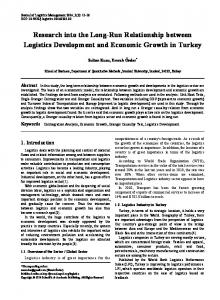
As briefly discussed above, the regime change in the PSTRVEC model is governed by the transition function F (∆gdpit −1; γ ; c ) . Here, the variables of interest are γ that determines the speed of transition between the extreme regimes, and c that determines the midpoint of the transition. The estimated value of cˆ = −0.00124 is very close to zero, which suggests that the extreme regimes in the PSTRVEC model (roughly) correspond to negative and positive values of the GDP growth rate, or to recessionary and expansionary regimes. In fact, the transition function F ( ∆gdpit −1 ; γ ; c ) takes on values less than 0.01 when lagged output growth rate is less than -1,5 and takes on values greater than 0,99 when the output growth rate is greater than 1,5. Therefore, the regimes identified by the transition function (roughly) correspond to recessionary regimes (i.e., when output growth rate is less than -1,5)
and expansionary regimes (i.e., when output growth rate is less than -1,5). The estimated value of
γˆ = 3.145 suggests that the transition between the regimes are rather smooth as can be seen from the Figure 1 below.
Estimated Transition Function
1.00
0.75
0.50
0.25
0.00 -7.5
-5.0
-2.5
0.0
2.5
5.0
7.5
10.0
Lagged Output Growth Rate
Figure 1. Scatter Plot of the Estimated Transition Function Against Transition Variable
Before proceeding to formal testing of the regime-wise Granger causality, we discuss the coefficient estimates for both output and energy consumption equations. First, consider the output equation. In the recessionary regime (i.e., when output growth rate is negative and thus, F ( ∆gdpit −1 ; γ ; c ) ≈ 0 ), the estimated coefficient of the error correction term is equal to -0.064, and is statistically insignificant. This result implies that output growth rate does not respond to the deviations from the long-run equilibrium level in recessionary regimes. The estimated coefficient of the lagged energy consumption is equal to 0.263 and is statistically significant only at 10% significance level. This implies that output growth rate increases with energy consumption in recessionary (or low-growth) regimes, although the evidence is (statistically) weak. In expansionary periods (i.e., when output growth rate is positive and thus, F ( ∆gdpit −1 ; γ ; c ) ≈ 1 ), the estimated coefficient of the error correction term becomes -0.070 (=-0.064-0.006) and remains statistically insignificant. The estimated coefficient of the lagged energy consumption turns to 0.241(=0.2630.022), implying the effect of energy consumption on output growth rate declines slightly in expansionary regimes.
Now, consider the energy equation. The estimated coefficient of the error correction term is equal to -0.151 and -0.218=(-0.151-0.067) in recessionary and expansionary regimes, respectively, and statistically significant in both regimes. This implies that energy consumption adjusts to disequilibrium both in recessionary and expansionary periods, whereas the speed of adjustment increases with output growth rate. The estimated coefficient of the output growth is equal to -0.015, and statistically insignificant in recessionary regime. In expansionary periods, it turns to 0.119 (=0.134-0.015) and becomes statistically significant, implying that output growth rate has no effect on energy consumption in recessionary regimes but increases it in expansionary regimes. Now we turn to the regime-wise Granger-causality tests. Vector error correction models provide a framework for testing Granger-causality for the short- and long-run relationships. Short-run Granger-causality test is performed through testing lagged values of explanatory variables, whereas the long-run causality is performed through the significance of the error-correction term. In addition, we also performed so-called stronger form of the Granger-causality, i.e., joint significance of the error correction term and lagged explanatory variables. As briefly discussed above, the PSTRVEC model allows for testing Granger-causality for each regime separately. Therefore, we performed the Grangercausality tests for the recessionary (i.e., when F (∆gdpit −1; γ ; c ) = 0 ) and expansionary (i.e., when F (∆gdpit −1 ; γ ; c ) = 1 ) regimes separately. The results of the regime-wise Granger-causality tests are reported below in Table 5.
Table 5. Regime-wise Causality Tests Dependent Variable Source of Causation (independent variable)
∆GDP
Recessionary Regime
∆ENR
Expansionary Regime
Recessionary Regime
Expansionary Regime
0.100 (0.750)
6.556** (0.037)
10.732* (0.001)
10.712* (0.004)
13.634* (0.001)
30.199* (0.000)
Short-Run ∆GDP ∆ ENR
2.817*** (0.093)
4.973*** (0.083)
Long-Run ECT
2.497 (0.114)
2.953 (0.228)
Joint (short- and long-run) ECT / ∆GDP ECT / ∆ENR
9.284* (0.009)
11.277** (0.023)
Notes: Figures in parenthesis denote p-values of the test statistics. *, ** and *** denote rejection of the null hypothesis of unit root at %1, % 5 and %10 significance levels, respectively. The results of the short run Granger causality tests suggest that energy consumption is a Granger cause of the output growth rate both in recessionary and expansionary regimes, although the evidence is statistically weak. Indeed, the null hypotheses that energy consumption does not Grangercause output growth is rejected for both regimes only at ten percent significance level. The results of the long-run Granger causality tests, on the other hand, imply that energy consumption does not cause output growth rate both in recessionary and expansionary regimes. Stronger (or joint) Granger causality tests suggest that energy consumption is a Granger-cause of output growth rate in both regimes. Combined with the results of the short- and long-run causality tests, the joint Granger causality test thus suggests that primary effect of the energy consumption on output growth stems from the short-run effects. As regards the energy consumption, the Granger causality tests suggest that output growth rate does not Granger-cause energy consumption in recessionary regimes but does Granger-cause it in expansionary regimes in the short-run. On the other hand, the results of the long-run and joint Granger causality tests suggest that output growth Granger causes energy consumption both in the recessionary and expansionary regimes. Our results have clear and nice policy implications. The results of the Granger-causality tests imply that energy consumption affects output growth rate only in the short run, irrespective of the phases of the business cycles. This finding suggests that the G7 countries can implement energy conversion policies without fear of harming long-run growth paths of the economies. Possible adverse effects of the energy conversion policies on output growth rate shall be limited to only short-run dynamics of the economy and such policies shall not harm the long run growth of the countries. This result also suggests that bad economic conditions (i.e., when the economy is in the recession or output growth rate is low) can not be considered as a hindrance for implementation of the environmentally friendly policies. In addition, we found that output growth rate does not increase energy consumption in the short run when initial growth rate is relatively low. However, output growth increases energy consumption in the long run irrespective of initial conditions of the economy. These results may be interpreted as an evidence of the fact that the technological change (or growth strategies) has been energy-intensive in these countries during the sample period. Therefore, all in all, our results imply that the energy conversion policies must be supplemented by policies aimed at promotion of energysaving technological progress.
4. Conclusion
In this paper, we have examined the causal relationship between total energy consumption and output level for a panel of G7 countries. The novelty of the paper is that we propose a new panel cointegration test in a nonlinear smooth transition regression framework and estimate nonlinear panel vector error correction model. Although conventional linear panel cointegration tests suggest that energy consumption and output level are not co-integrated, we find a strong evidence of cointegration among these variables using newly proposed nonlinear cointegration tests. This result suggests that adjustment of these variables to the long-run equilibrium level is inherently nonlinear. In order to estimate dynamics of the causal relationship between energy consumption and output level we then estimate a panel vector error correction model. Linearity tests suggest that the dynamic interrelationship between these variables is also nonlinear. Hence, we proceed to estimate a nonlinear smooth transition panel vector error correction model to estimate possible regime-dependent dynamics between energy consumption and output. The estimated nonlinear model suggests that the dynamic interrelationship between these variables depend on the phases of business cycle whereas the transition between the regimes is rather smooth. Then we conduct regime dependent Granger causality tests in order to see whether the causal relationship between the variables also varies across phases of the business cycle. The results of the Granger-causality tests can be summarized as follows. First, the energy consumption increases output growth rate in the short run both in economic recession and expansion periods, although the evidence is statistically weak. On the other hand, we find that energy consumption does not Granger-cause output in the long run irrespective of the initial conditions of the economy. Second, we find that output growth rate does not cause energy consumption in the short run in economic recession periods. In expansionary or high growth episodes, on the other hand, output growth rate increases energy consumption. In the long run, output growth increases energy consumption irrespective of initial conditions of the economy. Our results have several implications both for energy economists and policy authorities. Energy economists must take account of possible nonlinearities in examining causal relationship and dynamic interactions between variables. In particular, conventional linear models might be inappropriate in order to examine long run relationship between energy consumption and output growth rate. In addition to long-run relationships, we found a strong evidence of nonlinearity in shortrun dynamic interactions of the variables as well. Such regime dependent and nonlinear dynamics is also important for policy design. Policy authorities must take account of such nonlinearities and bear in mind that policy actions will affect economy in a nonlinear fashion. Our results imply that possible
negative effects of the energy conversion policies is limited to only short-run and therefore, policy authorities may implement environmentally friendly policies under all economic conditions without fear of harming long-run growth of the economy. In addition, energy-saving policies must be enhanced with policies aimed at promoting energy-efficient technological progress.
References
Aloui, C., Jammazi, R. 2009. The effects of crude oil shocks on stock market shifts behaviour: A regime switching approach. Energy Economics 31, 789-799
Akinlo, A.E., 2008. Energy consumption and economic growth: evidence from 11 Sub-Sahara African countries. Energy Economics 30 (5), 2391–2400.
Ang, J.B., 2008. Economic development, pollutant emissions and energy consumption in Malaysia. Journal of Policy Modeling 30, 271–278.
Apergis, N., Payne, J.E., 2009. Energy consumption and economic growth in Central America: evidence from a panel cointegration and error correction model. Energy Economics 31, 211–216.
Balcilar M., Ozdemir, Z.A., Arslanturk, Y., 2010. Economic growth and energy consumption causal nexus viewed through a bootstrap rolling window. Energy Economics 32, 1398-1410
Bai, J., Ng, S., 2004. A PANIC Attack on Unit Roots and Cointegration. Econometrica 72(4), 11271177.
Bai, J., Kao, C., Ng, S., 2009. Panel cointegration with global stochastic trends. Journal of Econometrics 149(1), 82-99.
Banerjee, A., Marcellino, M., Osbat, C., 2004. Some cautions on the use of panel methods for integrated series of macroeconomics data. Econometrics Journal, 7, 322-340.
Beaudreau, B.C., 2005. Engineering and economic growth. Structural Change and Economic Dynamics 16, 211–220.
Belloumi, M., 2009. Energy consumption and GDP in Tunisia: cointegration and causality analysis. Energy Policy 37 (7), 2745–2753.
Boden, T.A., G. Marland, and R.J. Andres. 2010. Global, Regional, and National Fossil-Fuel CO2 Emissions. Carbon Dioxide Information Analysis Center, Oak Ridge National Laboratory, U.S. Department of Energy, Oak Ridge, Tenn., U.S.A. doi 10.3334/CDIAC/00001_V2010.
Chang, Y., 2004. Bootstrap unit root tests in panels with cross-sectional dependency. Journal of Econometrics, 120(2), pages 263-293.
Cheng-Lang, Y., Lin, H.-P., Chang, C.-H., 2010. Linear and nonlinear causality between sectoral electricity consumption and economic growth: Evidence from Taiwan. Energy Policy Volume 38 (11), 6570-6573
Chiou-Wei, S.Z., Chen, Ching-Fu, Zhu, Z., 2008. Economic growth and energy consumption revisited—evidence from linear and nonlinear Granger causality. Energy Economics 30(6),3063– 3076.
Costantini, V., Martini, C., 2010. The causality between energy consumption and economic growth: A multi-sectoral analysis using non-stationary cointegrated panel data. Energy Economics 32, 591-603
Engle, R.F., Granger, C.W.J., 1987. Co-integration and error correction: representation, estimation, and testing. Econometrica 55: 251-276
Erdal, G., Erdal, H., Esengün, K., 2008. The causality between energy consumption and economic growth in Turkey. Energy Policy 36(10), 3838–3842.
Francis, B.M., Moseley, L., Iyare, S.O., 2007. Energy consumption and projected growth in selected Caribbean countries. Energy Economics 29, 1224–1232.
Gabreyohannes, E., 2010. A nonlinear approach to modelling the residential electricity consumption in Ethiopia. Energy Economics 32, 515-523
Ghali, K.H., El-Sakka, M.I.T., 2004. Energy use and output growth in Canada: a multivariate cointegration analysis. Energy Economics 26 (2), 225–238.
Glasure, Y.U., 2002. Energy and national income in Korea: further evidence on the role of omitted variables. Energy Economics 24, 355–365.
Gonzalez, A., Teräsvirta, T., Dijk, D. 2005. Panel smooth transition regression models, Working Paper Series in Economics and Finance No 604, Stockholm School of Economics, Sweden. Granger, C.W.J., Teräsvirta, T., 1993. Modelling nonlinear economic relationships. Advanced Texts in Econometrics. Oxford University Press, New York, USA.
Greene, W.H., 1997. Econometric Analysis, Third Edition. Prentice Hall, New Jersey, USA.
Halicioglu, F., 2009. An econometric study of CO2 emissions, energy consumption, income and foreign trade in Turkey. Energy Policy 37, 1156–1164.
Hamilton, J.D. 2003. What is an oil shock? Journal of Econometrics 113, 363-398
Hansen, B. 1999. Threshold effects in non-dynamic panels: estimation, testing and inference. Journal of Econometrics 93(2), 345-368
Hasanov, M., Telatar, E. 2011. A re-examination of stationarity of energy consumption: Evidence from new unit root tests. Energy Policy 39, 7726–7738
Heston, A., Summers, R., and Aten, B. (2009) Penn World Table Version 6.3. Center for International Comparisons of Production, Income and Prices at the University of Pennsylvania, August 2009.
Ho, C-Y., Siu, K.W., 2007. A dynamic equilibrium of electricity consumption and GDP in Hong Kong: an empirical investigation. Energy Policy 35 (4), 2507–2513.
Huang, B.N., Hwang, M.J. Yang, C.W., 2008. Does more energy consumption bolster economic growth? An application of the nonlinear threshold regression model. Energy Policy 36, 755-767
Im, K.S., Pesaran, H., Shin, Y., 2003. Testing for unit roots in heterogeneous panels. Journal of Econometrics 115, 53–74.
Kapetanios, G., Shin, Y., Snell, A. 2003. Testing for a unit root in the nonlinear STAR framework. Journal of Econometrics 112, 359-79.
Kapetanios, G., Shin, Y., Snell, A. 2006. Testing for cointegration in nonlinear smooth transition error correction models. Econometric Theory 22, 279-303.
Kapetanios, G., Pesaran, M. H., Yamagata, T. 2011. Panels with non-stationary multifactor error structures. Journal of Econometrics, 160(2), 326-348.
Kraft, J., Kraft, A., 1978. On the relationship between energy and GNP. Journal of Energy and Development 3, 401–403.
Lee, C.C., 2006. The causality relationship between energy consumption and GDP in G-11 countries revisited. Energy Policy 34, 1086–1093.
Lee, C.C., Chien, M.S., 2010. Dynamic modelling of energy consumption, capital stock, and real income in G-7 countries. Energy Economics 32, 564-581
Lee, C.C., Chang, C.P., 2007. Energy consumption and GDP revisited: a panel analysis of developed and developing countries. Energy Economics 29, 1206–1223.
Lee, C.C., Chang, C. P. 2008. Energy consumption and economic growth in Asian economies: A more comprehensive analysis using panel data. Resource and Energy Economics 30, 50–65
Li, J. 2006. Testing Granger causality in the presence of threshold effects. International Journal of Forecasting 22, 771–780.
Luukkonen, R., Saikkonen, P., Teräsvirta, T. 1988. Testing linearity against smooth transition autoregressive models. Biometrika 75, pp. 491-99
Maddala, G. S., Wu, S. 1999. A Comparative Study of Unit Root Tests with Panel Data and New Simple Test. Oxford Bulletin of Economics and Statistics 61, 631-652.
Maki, D. 2010. An alternative procedure to test for cointegration in STAR models. Mathematics and Computers in Simulation 80, 999-1006
Mehrara, M., 2007. Energy consumption and economic growth: the case of oil exporting countries. Energy Policy 35 (5), 2939–2945.
Moon, Y.S., Sonn, Y.H., 1996. Productive energy consumption and economic growth: an endogenous growth model and its empirical application. Resource and Energy Economics 18, 189–200.
Moon, H.R., Hyungsik, R., Perron, B., 2004. Testing for a unit root in panels with dynamic factors. Journal of Econometrics, 122(1), 81-126.
Narayan, P.K., Smyth, R., Prasad, A., 2007. Electricity consumption in the G7 countries: a panel cointegration analysis of residential demand elasticities. Energy Policy 35 (9), 4485–4494.
Narayan, P.K., Smyth, R., 2008. Energy consumption and real GDP in G7 countries: new evidence from panel cointegration with structural breaks. Energy Economics 30, 2331–2341.
Oh, W., Lee, K., 2004. Causal relationship between energy consumption and GDP: the case of Korea 1970–1999. Energy Economics 26 (1), 51–59.
Omay, T., Kan, E.O., 2010. Re-examining the Threshold Effects in the Inflation-Growth Nexus: OECD Evidence. Economic Modelling 27 (5), 995-1004.
Ozturk, I., 2010. A literature survey on energy–growth nexus. Energy Policy 38, 340–349.
Payne, J.E., 2009. On the dynamics of energy consumption and output in the US. Applied Energy 86 (4), 575–577.
Pedroni, P., 1999. Critical values for cointegration tests in heterogeneous panels with multiple regressors. Oxford Bulletin of Economic and Statistics 61, 653–678.
Pesaran, M.H. 2004. General diagnostic tests for cross-section dependence in panels. Cambridge Working Papers in Economics 0435, Faculty of Economics, University of Cambridge, UK.
Pesaran, M.H. 2007. A simple panel unit root test in the presence of cross-section dependence. Journal of Applied Econometrics 22(2), 265-312.
Rahman, S., Serletis, A. 2010 The Asymmetric Effects of Oil Price and Monetary Policy Shocks: A Nonlinear VAR Approach, Energy Economics 32, 1460-1466
Soytas, U., Sari, R., 2003. Energy consumption and GDP: causality relationship in G-7 countries and emerging markets. Energy Economics 25, 33–37.
Soytas, U., Sari, R., 2006. Energy consumption and income in G7 countries. Journal of Policy Modeling 28, 739–750
Stern, D.I., 2000. A multivariate cointegration analysis of the role of energy in the US macroeconomy. Energy Economics 22, 267–283.
Teräsvirta, T., 1994. Specification, estimation, and evaluation of smooth transition autoregressive models. Journal of the American Statistical Association 89, 208–218.
Teräsvirta, T., Anderson, H.M., 1992. Characterizing nonlinearities in business cycles using smooth transition autoregressive models. Journal of Applied Econometrics 7, S119–S136.
Uçar N. and Omay T.,(2009) “Testing For Unit Root In Nonlinear Heterogeneous Panels” Economics Letters. 104(1), 5-7.
Wolde-Rufael, Y., 2004. Disaggregated industrial energy consumption and GDP: the case of Shanghai. Energy Economics 26, 69–75.
Zachariadis, T., 2007. Exploring the relationship between energy use and economic growth with bivariate models: new evidence from G-7 countries. Energy Economics 29 (6), 1233–1253.
Zamani, M., 2007. Energy consumption and economic activities in Iran. Energy Economics 29 (6), 1135–1140.
Zhang, X.P., Cheng, X.M., 2009. Energy consumption, carbon emissions, and economic growth in China. Ecological Economics 68 (10), 2706–2712.